


1. Introduction
Self-propelled particles are ubiquitous in nature, with examples including Chlamydomonas reinhardtii (Polin et al. Reference Polin, Tuval, Drescher, Gollub and Goldstein2009), Escherichia coli (Lauga Reference Lauga2016) and Volvox (Drescher et al. Reference Drescher, Leptos, Tuval, Ishikawa, Pedley and Goldstein2009), among many others. Their motion in multiphase flows is primarily driven by internal forces, interactions with the surrounding fluid and external forces. This interplay results in behaviour significantly more complex than that of passive particles. Studying this dynamic is key to understanding self-propelled particles in multiphase systems, with important applications such as algae-based biohybrid microrobots for combating melanoma lung metastasis (Zhang et al. Reference Zhang2024), preventing and treating inflammatory bowel disease (Li et al. Reference Li and Nie2024) and removing SARS-CoV-2 from wastewater (Zhang et al. Reference Zhang2021).
Various mathematical models have been developed to study the motion of self-propelled particles, with the squirmer model being a widely adopted approach due to its simplicity and effectiveness in representing active swimmers. Originally introduced by Lighthill (Reference Lighthill1952) and then refined by Blake (Reference Blake1971a ,Reference Blake b ), the squirmer model prescribes slip velocities on the particle surface, allowing it to capture different swimming behaviours categorised as pullers, pushers or neutral squirmers. To validate the squirmer model’s effectiveness, Ito, Omori & Ishikawa (Reference Ito, Omori and Ishikawa2019) developed a ciliate model using a slender-body boundary integral method for comparison. Despite the squirmer model’s inability to account for internal energy dissipation, with over 90 % of the energy being lost within the cilia, it accurately predicts swimming speed, aligning well with the discrete ciliate model. Additionally, the integration of the squirmer model into lattice Boltzmann solvers has proven effective in capturing key features of squirmer dynamics across various scenarios (Kuron et al. Reference Kuron, Stärk, Burkard, De Graaf and Holm2019). Comprehensive reviews have also documented significant progress in the study of squirmer behaviour, encompassing hydrodynamic interactions, collective dynamics and different modelling techniques (Lauga & Powers Reference Lauga and Powers2009; Koch & Subramanian Reference Koch and Subramanian2011; Elgeti, Winkler & Gompper Reference Elgeti, Winkler and Gompper2015; Zöttl & Stark Reference Zöttl and Stark2023; Ishikawa Reference Ishikawa2024).
The behaviour of an individual squirmer in confined flows has been extensively studied. For example, Zöttl & Stark (Reference Zöttl and Stark2012) investigated a squirmer in cylindrical Poiseuille flow, showing that a puller tends to stabilise in an upstream orientation near the centre, whereas a pusher oscillates around the centreline with a defined amplitude. In terms of flow stability across various Reynolds numbers (0.01–1000), Chisholm et al. (Reference Chisholm, Legendre, Lauga and Khair2016) found that a pusher maintains steady axisymmetric flow up to
 $\textit{Re}$
= 1000, with swimming speed increasing steadily with
 $\textit{Re}$
, while a puller experiences flow instability at higher
 $\textit{Re}$
due to unsteady wake development, causing a decline in average swimming speed. Purushothaman & Thampi (Reference Purushothaman and Thampi2019) examined the behaviour of a squirmer in a two-dimensional (2-D) channel, finding that a strong puller or pusher tends to slide along the channel walls, while a weak puller remains near the centre and a weak pusher exhibits oscillatory motion spanning the channel width. Moreover, they concluded that the behaviour of a 2-D circular squirmer near a repulsive planar wall is qualitatively very similar to that of a three-dimensional (3-D) spherical squirmer. Extending this analysis, Ouyang & Lin (Reference Ouyang and Lin2021) used a 2-D squirmer model to simulate a microswimmer moving within a channel and identified four distinct locomotion modes: horizontal, attracted oscillatory, oscillatory and chaotic modes. Separately, Radhakrishnan et al. (Reference Radhakrishnan, Purushothaman, Dey and Thampi2024) investigated the trajectory of a squirmer in 3-D channels with square and rectangular cross-sections. The puller exhibits sliding motion within the channel, with weak puller sliding along the centreline and strong puller following paths close to the walls. The pusher typically follows a helical trajectory in square channels, while in rectangular channels, its motion becomes more complex but retains some similarities. In contrast, the neutral squirmer displays the most intricate trajectory, highly sensitive to initial conditions. Although there are differences between 2-D and 3-D simulations, many features observed in two dimensions can help inform the understanding of 3-D behaviours. Ishimoto (Reference Ishimoto2017) showed that an unsteady circular squirmer reproduces the same bifurcation structures and key wall-interaction dynamics as its 3-D spherical counterpart. Therefore, 2-D simulations remain a powerful and efficient means to capture fundamental microswimmer behaviours and to guide the design of microscale devices. Notable distinctions include the emergence of helical paths in three dimensions. Choudhary et al. (Reference Choudhary, Paul, Rühle and Stark2022) investigated the impact of fluid inertia on squirmers in Poiseuille flow, revealing that, in addition to the classical inertial lift, self-propulsion generates a swimming lift. This leads to complex bistable motion patterns, including the coexistence of tumbling with stable centreline swimming or swinging. Additionally, Dey et al. (Reference Dey, Buness, Hokmabad, Jin and Maass2022) revealed that even a spherical squirmer can exhibit oscillatory rheotaxis, a behaviour previously unobserved in artificial swimmers within microchannels, primarily driven by interactions with shear flow and the channel walls. Similarly, Omori et al. (Reference Omori, Kikuchi, Schmitz, Pavlovic, Chuang and Ishikawa2022) also demonstrated that Chlamydomonas reinhardtii exhibits rheotaxis, where the interplay between cyclic body deformation and swimming velocity enables orientation against the flow and migration towards the channel centre.
The influence of gravity and inertia also plays a significant role in squirmer dynamics. Rühle et al. (Reference Rühle, Blaschke, Kuhr and Stark2018) examined the behaviour of a squirmer subjected to gravity at low Reynolds numbers, revealing that the squirmer would either cruise when self-propulsion was dominant or remain stationary if gravitational forces prevailed. In addition, Fadda, Molina & Yamamoto (Reference Fadda, Molina and Yamamoto2020) investigated the sedimentation of a single squirmer near a flat surface, showing that introducing chirality caused the squirmer’s trajectory to shift from straight to circular with increasing chirality. Ouyang & Lin (Reference Ouyang and Lin2022) conducted numerical simulations on the sedimentation of a squirmer in a narrow vertical channel, identifying four distinct locomotive modes: vertical, attracted oscillatory, oscillatory and upward. And they highlighted that pushers tended to exhibit the upward mode at higher Reynolds numbers, while pullers swam faster at lower density ratios. However, Nie et al. (Reference Nie, Ying, Guan, Lin and Ouyang2023) reported five motion patterns of a single squirmer in a 2-D channel under finite fluid inertia, including steady downward falling, inclined falling or rising and small-scale or large-scale oscillations, noting that pushers settled more quickly than pullers.
Beyond individual dynamics, the interactions between pairs of squirmers are fundamental to understanding collective behaviour (Theers et al. Reference Theers, Westphal, Qi, Winkler and Gompper2018; Ishikawa, Brumley & Pedley Reference Ishikawa, Brumley and Pedley2021; Qi et al. Reference Qi, Westphal, Gompper and Winkler2022). The pioneering work by Ishikawa, Simmonds & Pedley (Reference Ishikawa, Simmonds and Pedley2006) established the basis for two-squirmer interactions. They derived analytical solutions for both small and large separation limits and validated their results with numerical simulations using a boundary-element method. Their study showed that squirmers attract each other at first, dramatically change orientation when in close contact and eventually separate. This avoidance and escape behaviour characteristic has also been further validated in related studies on bacteria (Ishikawa et al. Reference Ishikawa, Sekiya, Imai and Yamaguchi2007) and Paramecium (Ishikawa & Hota Reference Ishikawa and Hota2006). This dynamics is further influenced by passive and active terms in the fluid interaction, as noted by Pooley, Alexander & Yeomans (Reference Pooley, Alexander and Yeomans2007), leading to behaviours like attraction, repulsion or oscillation. Experimental observations of Volvox colonies have shown similar complexities, with swimming patterns resembling coordinated ‘dancing’ near surfaces (Drescher et al. Reference Drescher, Leptos, Tuval, Ishikawa, Pedley and Goldstein2009). After initially attracting each other, the colonies engaged in a motion resembling a ‘waltz’ or ‘minuet’, demonstrating the complex fluid interactions of squirmers. Li, Ostace & Ardekani (Reference Li, Ostace and Ardekani2016) numerically investigated the hydrodynamic interactions of squirmers in an unbounded fluid within a Reynolds number range of 0.1–100, demonstrating that fluid inertia decreases the contact time between two pushers, while a pair of pullers remains close for extended periods. Papavassiliou & Alexander (Reference Papavassiliou and Alexander2017) employed the Lorentz reciprocal theorem for Stokes flow to derive exact solutions for the motion of a squirmer near both planar and spherical no-slip boundaries, as well as for the hydrodynamic interactions between two squirmers. Their analysis captured arbitrary squirming motions and was applicable across all separations, revealing that the transition from near-field to far-field interactions occurs at a separation of approximately two squirmer diameters, with significant asymmetry emerging in the near field due to microstructural effects.
The nature of squirmer interactions has been explored extensively in various fluid environments and configurations, revealing how different conditions influence the behaviour. For instance, the interactions between two squirmers with finite and intermediate inertia in a stratified fluid were numerically investigated by More & Ardekani (Reference More and Ardekani2021). They reported that stratification eliminates the closed-loop trajectories observed for two pullers at intermediate fluid inertia and causes two pushers to come to a complete stop and stick together. Purushothaman & Thampi (Reference Purushothaman and Thampi2021) investigated the hydrodynamic collisions between squirmers and passive particles in microchannels. They found that the collisions were asymmetric, with the squirmer’s trajectory only altered in the intermediate stage, while the passive particle experienced displacement either towards or away from the channel walls. Ying et al. (Reference Ying, Jiang, Nie and Lin2022) used the lattice Boltzmann method to investigate the sedimentation of two squirmers in a 2-D vertical channel, identifying various motion modes for individual and paired squirmers. Their findings emphasised that the separation angle and swimming speed played significant roles in driving transitions between different locomotive patterns. Guan & Lin (Reference Guan and Lin2023) conducted simulations of the interactions between two squirmers in shear flow, revealing that pullers exhibit repulsive behaviour due to high-pressure regions forming between them, resulting in three distinct motion patterns: steady tilting motion, large-amplitude oscillation motion and small-amplitude oscillation motion. In contrast, pushers display five motion modes, including limit cycle motion and open limit cycle motion, which arise from differences in pressure distributions around them. Recently, Nie et al. (Reference Nie, Ying, Guan, Lin and Ouyang2023) found that interactions between pullers result in attraction, whereas pushers tend to repel each other. They also emphasised the intricate dynamics that arise between a puller and a pusher.
The geometry of squirmers significantly influences their motion (Li & Nie Reference Li and Nie2024; Guan, Ying & Lin Reference Guan, Ying and Lin2024), and this influence extends to their interactions with other squirmers. For example, Theers et al. (Reference Theers, Westphal, Gompper and Winkler2016) studied the dynamic scattering of a pair of spheroidal squirmers within a narrow slit between two flat surfaces, using the multiparticle collision dynamics method. They discovered that two pullers could swim cooperatively, forming a stable wedge-like conformation with a small constant angle. This outcome suggests that the anisotropic shape of spheroidal squirmers promotes wedge formation due to alignment tendencies dictated by their geometry. In contrast, for circular squirmers, the symmetric shape in two dimensions does not inherently support such alignment. This raises an intriguing question: Can circular squirmers still achieve a similar wedge-like arrangement despite the absence of geometric anisotropy? Our study aims to explore this possibility, investigating whether circular squirmers can form wedge-like configurations under specific conditions and identifying the factors that may enable this behaviour. Elucidating these robust, self-organised configurations not only deepens our understanding of the fundamental hydrodynamic interactions that govern collective squirmer dynamics but also informs the rational design of microscale robotic systems. This insight can ultimately lead to improved strategies for targeted drug delivery (Alapan et al. Reference Alapan, Yasa, Schauer, Giltinan, Tabak, Sourjik and Sitti2018), minimally invasive surgery and cancer treatments (Kong et al. Reference Kong, Gao, Wang, Fang and Hwang2023) in blood vessels by enabling more efficient coordination and control of microrobotic swarms.
The remainder of this paper is organised as follows. In § 2, we briefly introduce the direct numerical simulation method, including the lattice Boltzmann method, the squirmer model, the boundary conditions and the repulsive force model. The research problem, accompanied by schematic illustration and simulation parameters, is presented in § 3. In § 4, we analyse the simulation results under various parameter settings, emphasising the interactions and motion patterns of two squirmers. Finally, the conclusions and key findings are summarised in § 5.
2. Numerical method
2.1. Lattice Boltzmann method
In this paper, we adopt the widely used two-dimensional nine-velocity (D2Q9) single-relaxation time lattice Boltzmann method, based on the Bhatnagar–Gross–Krook collision operator, to solve fluid motion (Qian, d’Humières & Lallemand Reference Qian, d’Humières and Lallemand1992). For programming purposes, both the time step and the lattice spacing are chosen to be unity, that is,
 $\Delta t = \Delta x = 1$
. The discrete lattice Boltzmann equations are thus formulated as follows:
 \begin{equation} f_i(\boldsymbol{x}+\boldsymbol{e}_i, t + 1) = \left (1 - \frac {1}{\tau }\right )f_i(\boldsymbol{x}, t) + \frac {1}{\tau }f_i^{(0)}(\boldsymbol{x}, t),\qquad i=0,\,\ldots ,\,8, \end{equation}
where
 $f_i(\boldsymbol{x}, t)$
and
 $f_i^{(0)}(\boldsymbol{x}, t)$
are the discretised and equilibrium distribution functions at position
 $\boldsymbol{x} = (X, Y)$
with time
 $t$
along the
 $\boldsymbol{e}_i$
direction, respectively, and
 $\tau$
is the relaxation time. The fluid density and velocity can be determined by
 \begin{equation} \rho =\sum _i f_i(\boldsymbol{x}, t), \quad \rho \boldsymbol{u}=\sum _i \boldsymbol{e}_i f_i(\boldsymbol{x}, t). \end{equation}
For low-Mach-number flow, the Navier–Stokes equations can be derived by performing a Chapman–Enskog expansion (He & Luo Reference He and Luo1997).
2.2. Squirmer model
The squirmer model is widely used for simulating the hydrodynamic behaviour of self-propelled particles. Originally proposed by Blake (Reference Blake1971a ,Reference Blake b ), it describes the motion of self-propelled particles by introducing oscillatory fluctuations in the radial and tangential directions at the particle boundaries. The slip velocity at the squirmer’s surface can be represented as an infinite series expansion, combining radial and polar components. Typically, the radial component is neglected for simplicity, focusing instead on a second-order truncated tangential velocity model. Therefore, the tangential velocity is expressed as
 \begin{equation} \boldsymbol{U}^S(\theta )=\left (B_1 \sin \theta +B_2 \sin \theta \cos \theta \right ) \boldsymbol{\theta }=U^S \boldsymbol{\theta }. \end{equation}
Here,
 $\boldsymbol{\theta }$
refers to the polar unit vector for a given point on a squirmer’s surface,
 $U^S$
denotes the signed magnitude of the tangential velocity,
 $B_1$
influences the steady-state swimming velocity
 $U_s = B_1/2$
in Stokes flow, while
 $B_2$
determines the intensity of vorticity around the squirmer. A key parameter, called the squirmer-type factor
 $\beta$
, is introduced to classify squirmers into three categories: when
 $\beta \lt 0$
, the particle is classified as a pusher; when
 $\beta \gt 0$
, it is a puller; and when
 $\beta = 0$
, it is a neutral squirmer. For example, bacteria like Escherichia coli and Bacillus subtilis are typical pushers that propel themselves using flagella from their rear. In contrast, algae like Chlamydomonas reinhardtii are classic pullers that generate thrust from their front through a motion resembling frog swimming. Neutral squirmers, such as Volvox and Paramecium, do not produce vortices and exhibit symmetric streamlines. The tangential velocity distributions corresponding to various squirmer types are illustrated in figure 1. Overall, the squirmer model posits that self-propelled particles achieve motion by applying tangential velocities at their surfaces.
The tangential velocity distribution on the squirmer surface in polar coordinates, calculated using (2.3): (
 $a$
) pushers with
 $\beta = -5,-3,-1$
, (
 $b$
) neutral squirmer with
 $\beta = 0$
and (
 $c$
) pullers with
 $\beta = 5,3,1$
. The radial direction represents the dimensionless tangential velocity (
 $U^S/U_s$
) and the circumferential direction indicates the angle
 $\theta$
. Due to the vertical symmetry of the polar coordinate system, only the upper half is shown. The velocity is zero along the squirmer surface, negative inside the solid boundary and positive outside. Positive values indicate velocity in the same direction as
 $\boldsymbol{\theta }$
, while negative values are in the opposite direction. Red arrows at
 $\theta = \pi /4$
and
 $3\pi /4$
denote the tangential velocity direction, except for the cases of
 $\beta = \pm 1$
at
 $\theta = \pi /4$
.

2.3. Boundary conditions
The treatment of boundary conditions is essential for accurate simulations in the lattice Boltzmann method. The improved bounce-back scheme introduced by Lallemand & Luo (Reference Lallemand and Luo2003) effectively enforces no-slip boundary conditions on the surfaces of solid particles. This scheme enhances accuracy through an interpolation method, achieving second-order accuracy compared with the classical first-order bounce-back scheme. Following the collision step, a propagation process is executed for all fluid and solid nodes. Consequently, the distribution functions transferred from solid nodes to fluid nodes need to be updated according to the exact positions of the boundary nodes. As depicted in figure 2,
 $f_8$
of node
 $A$
is advected from the solid node
 $B$
during propagation. A parameter,
 $q=|AE|/|AB|$
, is introduced to determine the precise location of boundary node
 $E$
, allowing for the application of an interpolation method to update
 $f_8$
based on the values from neighbouring nodes:
 \begin{align} f_8(A)=\left \{ \begin{array}{ll} \displaystyle q(1+2q)f_6(B)+(1-4q^2)f_6(A)-q(1-2q)f_6(C)-f(E),&\displaystyle q\lt \frac {1}{2} \\[10pt] \displaystyle \frac {f_6(B)}{q(2q+1)}+\frac {(2q-1)f_8(C)}{q}-\frac {(2q-1)f_8(D)}{2q+1}-\frac {f(E)}{q(2q+1)}, &\displaystyle q\geqslant \frac {1}{2}. \end{array} \right .\nonumber\\[3pt] \end{align}
In the above,
 $f(E) = 2w_6\rho \boldsymbol{e}_6\cdot \boldsymbol{U}_E / c_s^2$
, where
 $w_8$
is the weight factor in the
 $\boldsymbol{e}_8$
direction, and
 $c_s=1/\sqrt {3}$
is the sound speed. Additionally, the velocity at the boundary node
 $E$
is adjusted to account for the squirmer’s self-propulsion:
 \begin{equation} \boldsymbol{U}_E=\boldsymbol{U}+\boldsymbol{\Omega } \times \boldsymbol{R}+\boldsymbol{U}^S, \end{equation}
where
 $\boldsymbol{U}$
and
 $\boldsymbol{\Omega }$
represent the translational and rotational velocities, respectively, and
 $\boldsymbol{R}$
denotes the position vector from the centroid of the squirmer to the boundary node
 $E$
. The forces and torques acting on the squirmer are calculated using a momentum-exchange scheme by examining each fluid–solid boundary link. The additional forces and torques arising from uncovered and covered fluid nodes during the squirmer’s motion should be considered (Aidun, Lu & Ding Reference Aidun, Lu and Ding1998).
In direct numerical simulations of multiphase flow involving particles, periodic boundary conditions are commonly applied at the inlet and outlet of channel flow. However, this approach does not accurately represent a specified number of particles; instead, it effectively simulates an infinite number of particles due to the periodicity. To address this limitation, this paper employs a dynamic mesh technique under non-periodic boundary conditions (Huang, Du & Zhu Reference Huang, Du and Zhu2021). Specifically, when the average position of all squirmers shifts beyond one lattice spacing, both the overall flow field and the squirmers are translated one lattice spacing in the opposite direction, ensuring that the squirmers remain within the computational domain. Given the nature of squirmers, which can move either with or against the fluid flow, necessitating consideration of dynamic meshes under these two conditions.
Improved bounce-back scheme boundary conditions. The blue circles represent the fluid nodes, while the green squares denote the solid nodes. The purple region in the upper left represents the squirmer, with its outline indicating the solid boundary. Node
 $A$
has neighbouring nodes
 $C$
and
 $D$
, which are the two closest adjacent nodes in the direction of
 $\boldsymbol{e}_8$
, whereas node
 $B$
is adjacent along the
 $\boldsymbol{e}_6$
direction. Node
 $E$
is the intersection of the line connecting nodes
 $A$
and
 $B$
with the particle boundary. Additionally,
 $f_1{-}f_8$
represent the distribution functions of node
 $A$
along the eight directions during the propagation process.

2.4. Repulsive force model
In the direct numerical simulation, two squirmers may collide. To prevent non-physical overlaps, the popular repulsive force model proposed by Glowinski et al. (Reference Glowinski, Pan, Hesla, Joseph and Periaux2001) is employed:
 \begin{equation} \boldsymbol{F}_{\textit{ij}}^p= \begin{cases} \boldsymbol{0}, & d_{\textit{ij}}\gt R_i+R_j+h_c \\[6pt] \displaystyle \frac {c_{\textit{ij}}}{\varepsilon _p}\left (\frac {R_i+R_j+h_c-d_{\textit{ij}}}{h_c}\right )^2 \frac {\boldsymbol{X}_i-\boldsymbol{X}_j}{d_{\textit{ij}}}, & d_{\textit{ij}} \leqslant R_i+R_j+h_c. \end{cases} \end{equation}
In this expression,
 $R_i$
and
 $R_j$
are the radii of these two squirmers, whose centroids are located at
 $\boldsymbol{X}_i$
and
 $\boldsymbol{X}_j$
, respectively. The distance between their centroids is denoted as
 $d_{\textit{ij}}=|\boldsymbol{X}_i-\boldsymbol{X}_j|$
. Distance
 $h_c$
is the cutoff distance, representing the threshold below which the repulsive force becomes active, which was set to be 1.5. The stiffness parameter
 $\varepsilon _p$
is chosen to keep the squirmers apart, while
 $c_{\textit{ij}}$
acting as a force scaling factor is determined by the difference between the squirmer’s gravitational and buoyancy forces in the simulation. Collisions between the squirmer and the solid wall may also occur, requiring a similar treatment:
 \begin{equation} \boldsymbol{F}_{\textit{ij}}^w= \begin{cases} \boldsymbol{0}, & d_{\textit{ij}}^{\prime }\gt R_i+R_{j}^{\prime }+h_c \\[6pt] \displaystyle \frac {c_{\textit{ij}}}{\varepsilon _w}\left (\frac {R_i+R_j^{\prime }+h_c-d_{\textit{ij}}^{\prime }}{h_c}\right )^2 \frac {\boldsymbol{X}_i-\boldsymbol{X}_j^{\prime }}{d_{\textit{ij}}^{\prime }}, & d_{\textit{ij}}^{\prime } \leqslant R_i+R_j^{\prime }+h_c. \end{cases} \end{equation}
Here,
 $R_j^{\prime }$
is the radius of the nearest imaginary squirmer located on the wall, with its centroid located at
 $\boldsymbol{X}_j^{\prime }$
and the distance given by
 $d_{\textit{ij}}^{\prime }=\boldsymbol{X}_i-\boldsymbol{X}_j^{\prime }$
. The stiffness coefficient
 $\varepsilon _w$
, used for collisions between the squirmer and the wall, is set to
 $10^{-3}$
, the same as
 $\varepsilon _p$
. Finally, by summing all the forces and torques acting on the squirmer, as described in § 2, the squirmer’s motion can then be determined using Newton’s second law.
3. Problem
As shown in figure 3, we systematically investigate the inertial migration and hydrodynamic interactions of two squirmers in channel flow to understand how they can stabilise into a stable wedge-like conformation. The fluid in the channel has a density
 $\rho$
and viscosity
 $\upsilon$
, with the squirmers having the same density, allowing them to remain suspended. A fully developed parabolic velocity profile is imposed at the channel inlet, while a constant pressure
 $p$
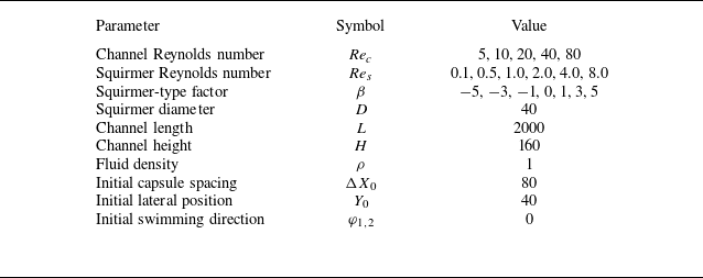
is set at the outlet. No-slip boundary conditions are applied on the upper and lower walls. As previously mentioned, dynamic mesh techniques are employed, and the midpoint of these two squirmers’ centroids stays near the channel centre in most cases. However, if their separation distance increases continuously during migration, they may move out of the channel. To gain better insights into the hydrodynamic interactions between two squirmers, we also examine the behaviour of a single squirmer under similar conditions. In the case of a single squirmer, it is initially positioned at the red dot shown in figure 3, with all other conditions remaining similar to those of the two-squirmer scenario. Table 1 provides a comprehensive overview of the simulation parameters, with values as indicated unless explicitly stated otherwise. Additionally, three key dimensionless numbers are essential for characterising the system’s dynamics. First, the channel Reynolds number is calculated using the expression
 \begin{equation} \displaystyle \textit{Re}_c = \frac {u_m H}{\upsilon }. \end{equation}
Schematic illustration of two squirmers in a channel with length
 $L$
and height
 $H$
. The velocity profile has a maximum velocity of
 $u_m$
. Initially, the midpoint of the squirmers’ centroids, marked by a red dot, is located at the coordinates (
 $X_0$
,
 $Y_0$
), with an initial centroid separation of
 $\Delta X_0$
. The subscript ‘0’ consistently denotes the initial value throughout this paper. The left squirmer (squirmer 1) and right squirmer (squirmer 2) have centroids at (
 $X_1$
,
 $Y_1$
) and (
 $X_2$
,
 $Y_2$
), respectively, with their initial positions satisfying
 $Y_1=Y_2=Y_0$
, and both have a diameter
 $D$
. The white arrows indicate their swimming directions, forming angles
 $\varphi _1$
and
 $\varphi _2$
with the
 $X$
axis. Simulation parameters are listed in table 1.

The parameters of two squirmers migrating in the channel. See figure 3 for an illustration of the set-up. The channel Reynolds number
 $\textit{Re}_c$
, squirmer Reynolds number
 $\textit{Re}_s$
and squirmer-type factor
 $\beta$
are calculated from equations (3.1), (3.2) and (3.3), respectively. All parameters are presented in simulation units. For instance, with a squirmer diameter of
 $D = 40$
, this implies the diameter is discretised into 40 lattice units, corresponding to
 $\Delta x / D = 0.025$
.

Values of
 $\textit{Re}_c$
listed in table 1 represent typical values found within vascular environments. Likewise, the squirmer Reynolds number is defined as
 \begin{equation} \displaystyle \textit{Re}_s = \frac {U_s D}{\upsilon }. \end{equation}
Lastly, the squirmer-type factor is determined by the ratio
 \begin{equation} \displaystyle \beta = \frac {B_2}{B_1}. \end{equation}
The three key parameters,
 $\textit{Re}_c$
,
 $\textit{Re}_s$
and
 $\beta$
, are varied across 5, 6 and 7 different values, respectively, as shown in table 1. Separate computations are performed for both single- and two-squirmer cases, resulting in a total of
 $5 \times 6 \times 7 \times 2 = 420$
cases to compute. In addition, supplementary calculations further increase the overall number of cases. To improve computational efficiency, a Python script has been developed for batch processing of these simulations.
4. Results and discussion
4.1. One squirmer
4.1.1. Regimes
To better understand the interactions between two squirmers in channel flow, a series of direct numerical simulations are first conducted for a single squirmer in the same flow environment. This approach allows for an isolated analysis of the squirmer’s behaviour and its response to the channel flow. A total of 210 parameter sets are studied, and the resulting data are analysed to identify key motion patterns, which are classified into four distinct motion modes, as shown in figure 4.
In figure 4(
 $a$
), for a typical parameter set with
 $\textit{Re}_s = 0.5$
,
 $\textit{Re}_c = 5$
and
 $\beta = -5$
, the squirmer exhibits oscillatory motion near the bottom wall of the channel. Initially, the squirmer swims to the right (first arrow), but the background flow, characterised by a parabolic velocity profile in the lower half of the channel, induces a clockwise torque, gradually shifting its swimming direction downward (second arrow). Because the value of
 $\textit{Re}_c$
is relatively low, the torque is insufficient to completely reverse the squirmer’s direction, so it continues downstream while approaching the wall. Upon contact with the bottom wall, the no-slip condition generates a lubrication force that applies a counterclockwise torque, causing the squirmer to rotate away from the wall. Inertia then drives the squirmer away from the wall, but the clockwise torque from the flow pulls it back, resulting in repeated downstream oscillations. Here, ‘downstream’ refers to the squirmer swimming in roughly the same direction as the background flow, while ‘upstream’ indicates a swimming direction roughly opposite to the flow. Specifically, when the angular difference between the squirmer’s swimming direction and the background flow is less than
 $\pi / 2$
or greater than
 $\pi / 2$
, it is considered downstream and upstream, respectively. Figure 4(
 $a$
) shows a typical case in regime I, where the squirmer exhibits downstream oscillations within the lower half of the channel. This regime includes all similar oscillatory behaviours, whether downstream, upstream or anomalous rolling oscillations, as long as the oscillatory motion stabilises within half of the channel.
Four representative regimes: (
 $a$
) regime I (
 $\textit{Re}_s = 0.5$
,
 $\textit{Re}_c = 5$
,
 $\beta = -5$
; see supplementary movie 1 available at https://doi.org/10.1017/jfm.2025.10277), (
 $b$
) regime II (
 $\textit{Re}_s = 0.5$
,
 $\textit{Re}_c = 20$
,
 $\beta = 5$
; see supplementary movie 2), (
 $c$
) regime III (
 $\textit{Re}_s = 0.5$
,
 $\textit{Re}_c = 20$
,
 $\beta = -5$
; see supplementary movie 3) and (
 $d$
) regime IV (
 $\textit{Re}_s = 1.0$
,
 $\textit{Re}_c = 5$
,
 $\beta = 3$
; see supplementary movie 4). Each subplot shows the trajectories of these two squirmers, with their swimming direction varying over time. The final moment’s horizontal velocity field is depicted alongside the squirmers, with white arrows indicating the swimming direction at that instant. Additionally, both the coordinates
 $X^\prime$
and
 $Y^\prime$
are made dimensionless by
 $X^\prime = X / H$
and
 $Y^\prime = Y / H$
, respectively, while time is normalised as
 $T^\prime = t U_s / D$
.

A different scenario is shown in figure 4(
 $b$
), where the parameters are
 $\textit{Re}_s = 0.5$
,
 $\textit{Re}_c = 20$
and
 $\beta = 5$
. Compared with figure 4(
 $a$
),
 $\textit{Re}_c$
increases from 5 to 20, and the squirmer type changes from a pusher (
 $\beta = -5$
) to a puller (
 $\beta = 5$
), while all other parameters remain unchanged. The higher channel Reynolds number increases the torque acting on the squirmer, resulting in a faster rotational velocity. Consequently, the squirmer transitions from downstream to upstream swimming before reaching the wall. As shown in figure 1(
 $c$
), as a puller, the slip velocity at its front is generally aligned with its swimming direction, while the slip velocity at its rear is mostly opposed to it. Since the magnitude of the front slip velocity is greater, the squirmer primarily swims upstream, with its front slip velocity remaining largely aligned with the flow. This configuration creates a counterflow at the rear, increasing the likelihood of vortex shedding near the tail and inducing oscillatory motion. As indicated by the second arrow in figure 4(
 $b$
), after transitioning to upstream swimming, the squirmer’s swimming direction tilts toward the upper wall, enabling it to cross the channel centreline. Upon crossing, the parabolic velocity profile in the upper half of the channel generates a counterclockwise torque, causing the squirmer to rotate counterclockwise. This rotation, combined with inertia, carries the squirmer to its maximum upward position before its swimming direction shifts towards the lower wall. Similarly, upon crossing back into the lower half of the channel, the flow applies a clockwise torque, rotating the squirmer clockwise and propelling it downward. This cyclic behaviour results in periodic oscillatory motion. Such oscillatory behaviour, characterised by crossing the channel centreline, is categorised as regime II. This includes various forms of oscillations involving centreline crossing, such as periodic oscillations reaching both walls or chaotic oscillations. The example in figure 4(
 $b$
) illustrates a specific case within this broader classification.
We now examine the scenario where
 $\textit{Re}_s = 0.5$
,
 $\textit{Re}_c = 20$
and
 $\beta = -5$
. As shown in figure 4(
 $c$
), the squirmer’s swimming direction transitions from downstream to upstream after an initial adjustment. Similar to the case in figure 4(
 $b$
), the high
 $\textit{Re}_c$
value facilitates this transition before the squirmer reaches the lower channel wall. Comparing figure 4(
 $c$
) with figure 4(
 $b$
), the swimming directions indicated by the third arrows are generally consistent. However, as shown in figure 1(
 $a$
), the front slip velocity of a pusher points forward, opposing the background flow. This opposition reduces the squirmer’s swimming speed and inertia, preventing it from crossing the channel centreline. Meanwhile, the rear slip velocity of a pusher points backward and has a greater magnitude than the front slip velocity. Since the rear slip velocity aligns with the background flow, it stabilises the upstream motion. Consequently, unlike the puller case, the pusher does not exhibit periodic oscillations but instead stabilises near one side of the channel. This behaviour is reminiscent of a passive particle, which can settle into a lateral equilibrium position. However, unlike a passive particle, which continues to rotate at its equilibrium position, a squirmer maintains a fixed upstream swimming direction. This tendency to stabilise at a lateral equilibrium position is classified here as regime III.
In the final regime of a single squirmer, referred to as regime IV, the squirmer either stabilises near the channel centreline or exhibits very small oscillations around it. This behaviour results from the interplay between the squirmer’s symmetric slip velocity distribution relative to its swimming direction and the symmetric flow field about the channel centreline, which minimises lateral disturbances and promotes stability. A specific example of this regime is presented in figure 4(
 $d$
) for
 $\textit{Re}_s = 1.0$
,
 $\textit{Re}_c = 5$
and
 $\beta = 3$
, where the symmetric surface velocity distribution aligns with the symmetric flow field, leading to a stable upstream swimming direction.
A polar phase diagram for a single squirmer, indicating four regimes (I
 $-$
IV), divided into five regions by
 $\textit{Re}_c$
: (
 $a$
)
 $\textit{Re}_c=5$
, (
 $b$
)
 $\textit{Re}_c=10$
, (
 $c$
)
 $\textit{Re}_c=20$
, (
 $d$
)
 $\textit{Re}_c=40$
and (
 $e$
)
 $\textit{Re}_c=80$
. The angular direction shows
 $\textit{Re}_s$
values of 0.1, 0.5, 1.0, 2.0, 4.0 and 8.0, while the radial direction spans
 $\beta$
values of −5, −3, −1, 0, 1, 3 and 5.

4.1.2. Phase diagram
Building on the previous introduction of four regimes, we now systematically analyse 210 cases for a single squirmer and classify the motion modes, as summarised in figure 5. When
 $\textit{Re}_s = 0.1$
and
 $\textit{Re}_c = 5$
or 10, as described earlier and illustrated in figure 1(
 $c$
), the higher slip velocity at the front of a puller with large
 $\beta$
aligns with the background flow, enhancing its inertia. This increased inertia allows the puller to cross the channel centreline and oscillate near it. As shown in figure 5, three cases fall into regime II, while the rest are classified as regime IV. As
 $\textit{Re}_c$
increases to 20, 40 or 80, all motion modes transition to regime I, irrespective of
 $\beta$
. Focusing on a specific case with
 $\textit{Re}_c = 20$
and
 $\beta = -5$
, we observe that as
 $\textit{Re}_s$
decreases further (see figure 6), the motion remains in regime I for all cases except when
 $\textit{Re}_s = 0$
, in which the squirmer behaves like a passive particle, with the final lateral equilibrium position showing excellent agreement with that reported by Wen et al. (Reference Wen, Li, Zhang and Fang2012). Figure 6(
 $a$
) shows that as
 $\textit{Re}_s$
decreases, the oscillation amplitude reduces, and the amplitude centre shifts further away from the channel centreline. Although no Fourier analysis is performed, figure 6(
 $a$
) and its inset suggest that the oscillation frequency increases as
 $\textit{Re}_s$
decreases. This increase in frequency can be attributed to the reduction in inertia at smaller
 $\textit{Re}_s$
, which consequently leads to a decrease in oscillation amplitude. Figure 6(
 $b$
) reveals that the rotational velocity increases with decreasing
 $\textit{Re}_s$
. This occurs because the squirmer moves farther from the channel centreline as
 $\textit{Re}_s$
decreases, encountering a stronger shear gradient from the background flow, which amplifies its rotational velocity.
(
 $a$
) Trajectories and (
 $b$
) swimming direction of the squirmer for different values of
 $\textit{Re}_s$
at
 $\textit{Re}_c = 20$
and
 $\beta = -5$
, where the dimensionless angle
 $\varphi ^\prime$
is defined as
 $\varphi / \pi$
. The inset in (
 $a$
) provides a zoomed-in view of the trajectory, and the legend in (
 $b$
) is shared with (
 $a$
).

Excluding cases with
 $\textit{Re}_s = 0.1$
, the remaining simulations reveal distinct trends in the distribution of regimes I and II based on
 $\textit{Re}_c$
,
 $\textit{Re}_s$
and
 $\beta$
. As shown in figure 5, for small
 $\textit{Re}_c$
(5 and 10), regime I tends to occur at small
 $\textit{Re}_s$
and strongly negative
 $\beta$
. Across all
 $\textit{Re}_c$
values considered, regime I also appears at large
 $\textit{Re}_s$
and strongly positive
 $\beta$
, though its frequency decreases as
 $\textit{Re}_c$
increases. In contrast, regime II is primarily observed at large
 $\textit{Re}_s$
with negative
 $\beta$
and small
 $\textit{Re}_s$
with positive
 $\beta$
. This behaviour arises from the interplay between inertia and flow interaction. For pushers at large
 $\textit{Re}_s$
, the opposing slip velocity at the squirmer’s front reduces the swimming speed, diminishing inertia and favouring a transition to regime II. Conversely, pullers at small
 $\textit{Re}_s$
experience enhanced inertia as their slip velocity aligns with the background flow, enabling them to overcome viscous resistance and cross the channel centreline. These observations highlight the role of inertia, modulated by
 $\textit{Re}_s$
and
 $\beta$
, in determining the dynamics. For regime II, achieving centreline-crossing oscillations requires an optimal balance of inertia.
For a neutral squirmer (
 $\beta = 0$
), figure 1(
 $b$
) shows that the slip velocity is zero at the head and tail but aligns with the
 $\theta$
-angle direction elsewhere, generally opposing the swimming direction. The symmetry of the background flow about the channel centreline allows the squirmer to stabilise near this centreline. In this stable position, the slip velocity aligns with the background flow, resulting in an upstream swimming state closely following the channel centreline. When
 $\beta = -1$
, the maximum slip velocity shifts towards the tail, whereas for
 $\beta = 1$
, it shifts towards the head, as depicted in figures 1(
 $a$
) and 1(
 $c$
), respectively. Despite these differences, the slip velocity generally follows the
 $\theta$
-angle direction and rarely becomes negative. Consequently, the squirmer’s stable position remains near the channel centreline, similar to the neutral case. However, for
 $\beta = 1$
, the slip velocity near the front aligns with the background flow. This configuration is less stable compared to the case where the rear slip velocity aligns with the flow, as it tends to form periodic vortex shedding more easily. These instabilities result in slight oscillations around the channel centreline. These observations explain why squirmers with
 $\beta = -1$
, 0 and 1 frequently exhibit regime IV, as illustrated in figure 5.
Regime III, as shown in figure 5, is characterised by sporadic occurrences for pullers but appears more frequently for pushers, especially at larger absolute values of
 $\beta$
. This tendency to emerge at large
 $\lvert \beta \rvert$
is attributed to the stronger resistance such a squirmer provides against the shear torque generated by the background flow, allowing it to stabilise at specific swimming angles. For pushers, the interaction between their slip velocity and the background flow plays a crucial role. The alignment of the rear slip velocity with the flow reduces vertical shear and enhances stability, making regime III more likely. At higher
 $\textit{Re}_c$
, stronger inertial effects and reduced shear fluctuations further enhance this tendency. As illustrated in figure 7, a pusher, regardless of whether it exhibits regime I or III, tends to align its swimming direction towards the channel centreline, while a puller consistently orients towards the solid wall. For pushers, at lower channel Reynolds numbers (
 $\textit{Re}_c = 5$
, 10), the background flow’s shear torque is insufficient to reverse the downstream swimming direction, resulting in sustained oscillatory motion near the wall, characteristic of regime I. As
 $\textit{Re}_c$
increases to 20, regime III emerges. In contrast, pullers predominantly maintain an upstream swimming state in both regimes I and III, regardless of
 $\textit{Re}_c$
, although downstream swimming may occasionally occur. Their front slip velocity drives fluid towards them, creating an attractive effect that pulls them towards the wall. Consequently, their swimming direction consistently inclines towards the solid boundary, whether they are swimming upstream or downstream.
Streamlines and X-direction velocity contours around squirmers with
 $\textit{Re}_s = 1.0$
for varying
 $\beta$
and
 $\textit{Re}_c$
: (
 $a {-} c$
)
 $\beta = -5$
, (
 $d {-} f$
)
 $\beta = 5$
; (
 $a,d$
)
 $\textit{Re}_c = 5$
, (
 $b,e$
)
 $\textit{Re}_c = 10$
, (
 $c,f$
)
 $\textit{Re}_c = 20$
.

Seven representative regimes: (
 $a$
) regime A (
 $\textit{Re}_s = 0.5$
,
 $\textit{Re}_c = 5$
,
 $\beta = -5$
; see supplementary movie 5), (
 $b$
) regime B (
 $\textit{Re}_s = 0.5$
,
 $\textit{Re}_c = 20$
,
 $\beta = 5$
; see supplementary movie 6), (
 $c$
) regime C (
 $\textit{Re}_s = 0.5$
,
 $\textit{Re}_c = 20$
,
 $\beta = -5$
; see supplementary movie 7), (
 $d$
) regime D (
 $\textit{Re}_s = 0.5$
,
 $\textit{Re}_c = 20$
,
 $\beta = 1$
; see supplementary movie 8), (
 $e$
) regime E (
 $\textit{Re}_s = 2.0$
,
 $\textit{Re}_c = 5$
,
 $\beta = 0$
; see supplementary movie 9), (
 $f$
) regime F (
 $\textit{Re}_s = 1.0$
,
 $\textit{Re}_c = 10$
,
 $\beta = 3$
; see supplementary movie 10) and (
 $g$
) regime G (
 $\textit{Re}_s = 1.0$
,
 $\textit{Re}_c = 5$
,
 $\beta = 3$
; see supplementary movie 11). Each subplot shows the trajectories of these two squirmers, with their swimming direction varying over time. The final moment’s horizontal velocity field is depicted alongside the squirmers, with white arrows indicating the swimming direction at that instant.

4.2. Two squirmers
4.2.1. Regimes
After analysing the motion of a single squirmer, we now shift our focus to the behaviour of two squirmers under identical parameter conditions. A detailed investigation of 210 cases identifies seven representative regimes for two squirmers, summarised in figure 8. Comparing these regimes with the single-squirmer results in figure 4 reveals a clear correspondence between the regimes of a single squirmer and those of two squirmers for the same parameter combinations. For instance, figure 8(
 $a$
) highlights that the single squirmer’s regime I aligns with the two-squirmer regime A, characterised by
 $\textit{Re}_s = 0.5$
,
 $\textit{Re}_c = 5$
and
 $\beta = -5$
. In regime A, both squirmers oscillate within one half of the channel, either together or in opposite halves of the channel, replicating the oscillatory behaviour observed in regime I. Similarly, figure 8(
 $b$
) illustrates that regime II for a single squirmer corresponds to regime B for two squirmers, defined by
 $\textit{Re}_s = 0.5$
,
 $\textit{Re}_c = 20$
and
 $\beta = 5$
. In regime B, both squirmers display oscillatory motion that spans the channel centreline. Although the oscillatory trajectories are less sinusoidal compared with the single squirmer’s motion shown in figure 4(
 $b$
), this deviation is attributed to the interaction between the two squirmers. The interactions minimally influence the overarching motion patterns, with channel centreline crossing remaining a defining feature, closely aligned with the dynamics of regime II. Figure 8(
 $c$
) further demonstrates that regime III of the single squirmer corresponds to regime C for two squirmers, with
 $\textit{Re}_s = 0.5$
,
 $\textit{Re}_c = 20$
and
 $\beta = -5$
. In regime C, both squirmers stabilise at lateral equilibrium positions within one half of the channel, maintaining a tilted swimming orientation. This behaviour is consistent with regime III, whether the squirmers occupy the same or opposite halves of the channel. Additionally, figure 8(
 $e$
) shows that regime IV for a single squirmer corresponds to regime E for two squirmers, with
 $\textit{Re}_s = 2.0$
,
 $\textit{Re}_c = 5$
and
 $\beta = 0$
. Both cases exhibit upstream stabilisation near the channel centreline. These comparisons confirm that the two squirmers’ motion retains the key characteristics of the single-squirmer regimes. For several parameter combinations, regime I corresponds to regime A, regime II to regime B, regime III to regime C and regime IV to regime E. In these cases, the interaction between the two squirmers minimally influences their overall motion patterns, resulting in a direct correspondence between the single- and two-squirmer regimes.
Figure 8(
 $d$
) Illustrates the main interesting dynamic behaviour explored in this study, identified as regime D, where two circular squirmers eventually stabilise into a wedge-like conformation under the parameters
 $\textit{Re}_s = 0.5$
,
 $\textit{Re}_c = 20$
,
 $\beta = 1$
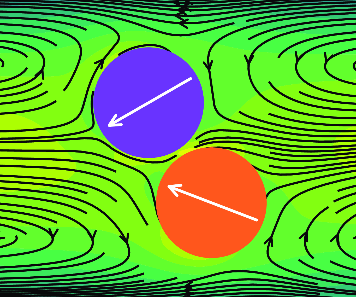
. To provide a comprehensive understanding of how this conformation develops, figure 9 presents a detailed sequence of the transition process. Under these parameters, a single squirmer typically stabilises near the channel centreline, corresponding to regime IV, as demonstrated in figure 5. When two squirmers are introduced under identical conditions, they initially align along the channel centreline. However, for
 $\beta = 1$
, corresponding to a puller, the slip velocity distribution around its front and rear drives fluid towards itself. This hydrodynamic effect induces a mutual attraction between the two pullers, causing them to gradually approach each other, as shown in figures 9(
 $a$
) and 9(
 $b$
). Eventually, they come into physical contact, as depicted in figure 9(
 $c$
). As previously noted, the slip velocity distribution of pullers results in inherently less stable motion compared to pushers. This instability causes a single puller to exhibit small oscillations, frequently deviating from the channel centreline. For two pullers, as illustrated in figure 9(
 $d$
), squirmer 2 becomes noticeably destabilised and moves underneath squirmer 1. Simultaneously, squirmer 2 is lifted, forming a preliminary wedge-like arrangement. Their swimming directions then stabilise, both pointing towards the bifurcation of the upstream flow, as shown in figure 9(
 $e$
). Finally, after further minor adjustments, the two squirmers ultimately establish a stable wedge-like conformation, as presented in figure 8(
 $d$
).
Instantaneous streamlines and X-direction velocity contours around two squirmers at different times, illustrating the formation of regime D: (
 $a$
)
 $T^\prime = 36.46$
, (
 $b$
)
 $T^\prime = 39.06$
, (
 $c$
)
 $T^\prime = 41.67$
, (
 $d$
)
 $T^\prime = 44.27$
and (
 $e$
)
 $T^\prime = 46.88$
. The X-direction velocity is normalised as
 $u_x^\prime = u_x / u_m$
. The parameters are set as
 $\textit{Re}_s = 0.5$
,
 $\textit{Re}_c = 20$
and
 $\beta = 1$
.

The trajectories of the two squirmers in figure 8(
 $f$
) under the parameter combination
 $\textit{Re}_s = 1.0$
,
 $\textit{Re}_c = 10$
and
 $\beta = 3$
exhibit highly chaotic behaviour. Their motion alternates between downstream and upstream swimming, with prolonged irregular movement throughout the channel and frequent crossings of the channel centreline. Figure 10 provides a detailed analysis to further illustrate their dynamics. In figure 10(
 $a$
), during the initial stage, both squirmers exhibit clockwise rotational motion. However, because squirmer 2 is located within the trailing vortex of squirmer 1, it experiences a weaker torque. As a result, squirmer 1 rotates one additional full circle compared with squirmer 2. In subsequent motion, both squirmers predominantly swim upstream. For squirmer 1, upstream swimming occurs more frequently in the interval
 $-3.5 \lt \varphi ^\prime \lt -2.5$
, while rare downstream swimming occurs within
 $-4 \lt \varphi ^\prime \lt -3.5$
and
 $-2.5 \lt \varphi ^\prime \lt -2$
. Similarly, squirmer 2 exhibits upstream swimming primarily in the range
 $-1.5 \lt \varphi ^\prime \lt -0.5$
, with less frequent downstream swimming observed in the intervals
 $-2 \lt \varphi ^\prime \lt -1.5$
and
 $-0.5 \lt \varphi ^\prime \lt 0$
. Additionally, the trajectories in the phase plane (
 $\varphi ^\prime$
,
 $Y^\prime$
), as shown in figure 10(
 $a$
), are remarkably similar for both squirmers. These trajectories reveal three distinct behaviours: upstream swimming near the channel centreline, inclination towards the bottom wall in the lower half of the channel and inclination towards the top wall in the upper half of the channel. These inclinations are consistent with the behaviour of pullers shown in figure 7(
 $d {-} f$
). Figure 10(
 $b$
) depicts the relative trajectory of squirmer 2 with respect to squirmer 1, where squirmer 1 is fixed at the origin (represented by the purple circle). Initially, squirmer 2 is located to the right of squirmer 1. Due to the slip velocity distribution characteristic of pullers, the two squirmers experience mutual hydrodynamic attraction, leading to frequent collisions and position exchanges. Although inertia may cause the squirmers to temporarily move apart, the hydrodynamic interactions pull them back together. The black dashed circle in figure 10(
 $b$
) represents the maximum extent that squirmer 2 can reach around squirmer 1. It is evident that their collisions predominantly occur at their front and rear sides, while collisions at the top and bottom sides are rare.
Representative case of regime F with parameters
 $\textit{Re}_s = 1.0$
,
 $\textit{Re}_c = 10$
,
 $\beta = 3$
. (
 $a$
) Trajectories of two squirmers in the phase plane (
 $\varphi ^\prime$
,
 $Y^\prime$
). (
 $b$
) The relative trajectory of squirmer 2 with respect to squirmer 1, where the purple circle represents squirmer 1 at the origin. The black dashed circle indicates the boundary of the maximum reachable position for the centre of mass of squirmer 2 around squirmer 1. In both subplots, the trajectory colour evolves over time.

Figure 8(
 $g$
) illustrates the final motion mode, regime G, for the interaction between two squirmers at
 $\textit{Re}_s = 1.0$
,
 $\textit{Re}_c = 5$
and
 $\beta = 3$
. In this regime, the squirmers move apart and eventually exit the simulation domain, terminating the numerical simulation. Under these conditions, squirmer 1 exhibits motion consistent with regime IV for a single squirmer, swimming upstream along the channel centreline, while squirmer 2 transitions into regime I, oscillating downstream in the lower half of the channel. The faster downstream swimming speed of squirmer 2 compared with the upstream swimming speed of squirmer 1 leads to their increasing separation. For a single squirmer at the same parameter combination, as shown in figure 5(
 $a$
), regime IV is typically observed. However, in the two-squirmer case, regime E does not emerge, likely due to interactions and collisions in the early stages of figure 8(
 $g$
). These interactions cause squirmer 2 to reorient its swimming direction towards the lower wall, leading to oscillatory motion near the wall and a transition into regime I. This suggests that the initial swimming angle plays a role in determining the final motion mode of a squirmer.
To investigate the effect of the initial swimming angle, simulations were conducted for a single squirmer released at the same initial position (
 $Y^\prime = 0.25$
) with varying initial swimming angles, as shown in figure 11. Starting from
 $\varphi ^\prime = 0$
, the initial swimming angle is incremented by 0.25 in each case. The results indicate that only when
 $\varphi ^\prime = 1.75$
does the squirmer exhibit regime I, while for all other initial swimming angles, it transitions into regime IV. Figure 11(
 $a {-} c$
) further reveals that the squirmer crosses the channel centreline once only when
 $\varphi ^\prime = 0.25$
, 0.5 or 0.75. Among these trajectories, since
 $\varphi ^\prime = 1.75$
corresponds to the squirmer swimming downstream, its displacement is the largest. For the other cases, which all involve upstream swimming, the displacement is the largest for
 $\varphi ^\prime = 0.25$
and the smallest for
 $\varphi ^\prime = 1.25$
. These findings highlight that the initial swimming angle may influence the final motion mode of a squirmer, even when released from the same initial position.
Trajectories and evolution of swimming directions for a squirmer under different initial swimming directions: (
 $a$
)
 $\varphi _0^\prime = 0$
, (
 $b$
)
 $\varphi _0^\prime = 0.25$
, (
 $c$
)
 $\varphi _0^\prime = 0.5$
, (
 $d$
)
 $\varphi _0^\prime = 0.75$
, (
 $e$
)
 $\varphi _0^\prime = 1$
, (
 $f$
)
 $\varphi _0^\prime = 1.25$
, (
 $g$
)
 $\varphi _0^\prime = 1.5$
and (
 $h$
)
 $\varphi _0^\prime = 1.75$
. The other parameters used,
 $\textit{Re}_s = 1.0$
,
 $\textit{Re}_c = 5$
and
 $\beta = 3$
, are consistent with those of the representative case shown in figure 8, where two squirmers eventually evolve into regime G. Note that (
 $h$
) only shows the lower half of the channel, and the range of
 $X^\prime$
coordinates displayed is different from that in the other subfigures.

(
 $a$
) Trajectories of a squirmer from different initial positions for
 $\varphi _0^\prime = 1.75$
only and (
 $b$
) trajectories in the phase plane (
 $\varphi ^\prime$
,
 $Y^\prime$
) for various initial angles
 $\varphi _0^\prime = 0.25, 0.5, 0.75, 1.0, 1.25, 1.5, 1.75, 2.0$
. The other parameters are consistent with figure 11(
 $h$
), where
 $\textit{Re}_s = 1.0$
,
 $\textit{Re}_c = 5$
and
 $\beta = 3$
. The legend in (
 $a$
) is shared with (
 $b$
), representing different initial heights
 $Y_0^\prime$
. Markers indicate the positions where the squirmer is initially released. Due to symmetry, simulations are conducted only for initial positions
 $Y_0^\prime$
in the lower half of the channel and at the centreline. In the inset of (
 $b$
), three stable fixed points,
 $L_1$
,
 $L_2$
and
 $L_3$
, are shown. An unstable limit cycle, indicated by the black dashed line, is present in the lower right and contains a stable limit cycle
 $L_4$
. By symmetry, a corresponding unstable limit cycle and stable limit cycle
 $L_5$
are expected in the upper left.

In the previous discussion, we noted that the initial swimming angle influences a squirmer’s motion mode when its initial release position is fixed. This naturally raises the question: if the swimming angle is held constant, could different release positions also affect the squirmer’s motion mode? Figure 12(
 $a$
) shows the trajectories of a squirmer with a fixed initial swimming angle,
 $\varphi _0^\prime = 1.75$
, for various initial release positions,
 $Y_0^\prime$
. The simulations reveal that when
 $Y_0^\prime \leqslant 0.25$
, the squirmer exhibits regime I, while for all other cases, the motion evolves into regime IV. Notably, in regime IV, the stable positions of the squirmers do not align exactly with the channel centreline. For simplicity, all cases stabilising near the centreline are categorised as regime IV without further sub-classification. In regime I, the stable trajectories display consistent oscillation frequencies and amplitudes, suggesting the presence of a potential limit cycle. To investigate the combined influence of initial release position and swimming angle, figure 12(
 $b$
) presents the trajectories in the phase plane (
 $\varphi ^\prime$
,
 $Y^\prime$
), encompassing all combinations of predefined initial release positions and swimming angles in the lower half of the channel, including the channel centreline (
 $8 \times 8 = 64$
cases). Since
 $\varphi _0^\prime = 0$
and
 $\varphi _0^\prime = 2.0$
are equivalent, cases with
 $\varphi _0^\prime = 0$
are plotted at
 $\varphi _0^\prime = 2.0$
to facilitate interpretation. The inset of figure 12(
 $b$
) reveals three fixed points (
 $L_1$
,
 $L_2$
,
 $L_3$
): one located at (
 $\varphi ^\prime = 1.0$
,
 $Y^\prime = 0.5$
), representing a squirmer swimming upstream exactly along the channel centreline, and two slightly offset from this central point. As noted earlier, all three fixed points are categorised as regime IV. Additionally, figure 12(
 $b$
) highlights the presence of an unstable limit cycle (dashed black line) and a stable limit cycle (
 $L_4$
) in the lower right corner of the phase plane. Due to symmetry, if the squirmer is released from the upper half of the channel, a corresponding unstable limit cycle and stable limit cycle (
 $L_5$
) would appear in the upper left corner of the phase plane. For cases outside the unstable limit cycle, the squirmer evolves into regime IV, whereas cases within the unstable limit cycle transition into regime I. Furthermore, all trajectories that begin within the unstable limit cycle eventually stabilise on the stable limit cycle. This explains why, after several collisions, one squirmer enters the region within an unstable limit cycle and transitions into regime I, while the other remains outside the unstable limit cycle and evolves into regime IV. Consequently, the distance between the two squirmers gradually increases, ultimately leading to regime G, as illustrated in figure 8(
 $g$
).
A polar phase diagram for two squirmers illustrates seven regimes (A–G), organised into five regions by
 $\textit{Re}_c$
: (
 $a$
)
 $\textit{Re}_c=5$
, (
 $b$
)
 $\textit{Re}_c=10$
, (
 $c$
)
 $\textit{Re}_c=20$
, (
 $d$
)
 $\textit{Re}_c=40$
and (
 $e$
)
 $\textit{Re}_c=80$
. The angular direction represents
 $\textit{Re}_s$
values of 0.1, 0.5, 1.0, 2.0, 4.0 and 8.0, and the radial direction covers
 $\beta$
values of −5, −3, −1, 0, 1, 3 and 5.

4.2.2. Phase diagram
After analysing 210 two-squirmer cases, their motion modes are classified and summarised in figure 13. Compared with the single-squirmer phase diagram in figure 5, intriguing relationships and evolutionary patterns emerge. Regimes A, B and C for two squirmers largely correspond to regimes I, II and III for a single squirmer, respectively, suggesting that fundamental behaviours such as stable oscillations or steady states persist despite the complexity introduced by hydrodynamic interactions. In contrast, regime IV for a single squirmer evolves into distinct dynamics in two-squirmer systems, giving rise to regimes D, E and F, driven by interactions like collisions and slip velocity distributions. For instance, with
 $\beta = 1$
, nearly all cases (except
 $\textit{Re}_c = 5$
) stabilise into regime D, characterised by a wedge-like configuration primarily due to the attractive interactions between pullers. For
 $\beta = 0$
and
 $\beta = -1$
, the squirmers predominantly transition into regime E, where both squirmers remain stably upstream near the channel centreline, primarily due to the symmetric slip velocity distribution of the squirmers. Regime F, however, is rare, observed only for specific combinations of
 $\textit{Re}_c$
and
 $\textit{Re}_s$
, such as
 $\textit{Re}_c = 5$
,
 $\textit{Re}_s = 0.5$
and
 $\textit{Re}_c = 10$
,
 $\textit{Re}_s = 1.0$
. A notable feature is the emergence of regime G, where squirmers diverge indefinitely due to hydrodynamic interactions. Remarkably, any single-squirmer regime can transition into regime G in two-squirmer dynamics, highlighting how the interactions between the squirmers can lead them to enter different single-squirmer motion modes, causing them to move apart. Such evolutionary relationships underscore how the addition of a second squirmer introduces complex interplays of forces, creating new regimes and altering the stability of existing ones, in contrast to the simpler dynamics of single squirmers.
Although many cases with
 $\beta = 0$
and
 $\beta = -1$
stabilise in regime E, figure 14 highlights key differences under the parameters
 $\textit{Re}_s = 1.0$
and
 $\textit{Re}_c = 40$
. In the (
 $\varphi ^\prime$
,
 $Y^\prime$
) phase plane, figure 14(
 $c$
) shows slight variations in the trajectories, with all squirmers starting at (0, 0.25) and converging near (−1.0, 0.5). Figure 14(
 $d$
) reveals that the distance
 $\Delta X^\prime$
stabilises over time, with
 $\Delta X^\prime$
being larger for
 $\beta = -1$
than for
 $\beta = 0$
, indicating distinct hydrodynamic interactions. For
 $\beta = 0$
, the symmetric slip velocity distribution generates balanced interactions, resulting in stable configurations with minimal horizontal displacement, as illustrated by the streamlines in figure 14(
 $a$
). In contrast, for
 $\beta = -1$
as shown in figure 14(
 $b$
), the slip velocity distribution creates a repulsive effect, pushing fluid away from the right side of squirmer 1. This flow behaviour leads to a repulsion between the squirmers, causing a larger
 $\Delta X^\prime$
.
Cases illustrating regime E, with
 $\textit{Re}_s = 1.0$
,
 $\textit{Re}_c = 40$
and
 $\beta = 0, -1$
. Streamlines and X-direction velocity contours around two squirmers at
 $T^\prime = 1562.5$
for (
 $a$
)
 $\beta = 0$
and (
 $b$
)
 $\beta = -1$
. In (
 $a$
,
 $b$
), squirmer 1 (purple) and squirmer 2 (orange) are shown, with the white arrows indicating their stable swimming directions. (
 $c$
) Trajectories of squirmers in the (
 $\varphi ^\prime$
,
 $Y^\prime$
) phase plane. (
 $d$
) Time evolution of
 $\Delta X^\prime$
and
 $\Delta Y^\prime$
, representing the X- and Y-direction distances between squirmer 2 and squirmer 1, respectively.

A careful comparison of figures 5 and 13 reveals that the motion modes of a single squirmer and two squirmers under the same parameter combinations do not exhibit the previously mentioned correspondence. For instance, as shown in figure 15 under parameters
 $\textit{Re}_s = 8.0$
,
 $\textit{Re}_c = 5$
and
 $\beta = 3$
, the single squirmer exhibits regime I, whereas the two squirmers display regime C. In figure 15(
 $b$
), the single squirmer demonstrates stable oscillatory motion characterised by two distinct limit cycles. The smaller limit cycle corresponds to downstream swimming, while the larger one occurs during upstream swimming. These cycles are connected by sliding motions near the wall, alternating periodically. Since
 $\beta = 3$
indicates a puller, the squirmer experiences an attractive interaction with the lower wall, causing its orientation to consistently tilt towards it. The trajectory in figure 15(
 $a$
) further illustrates that during the smaller limit cycle, the squirmer moves in the positive Xdirection, while in the larger limit cycle it moves in the negative Xdirection, resulting in periodic oscillatory motion. For the case of two squirmers, as shown in figures 15(
 $d$
) and 15(
 $f$
), they initially exhibit oscillatory motions reminiscent of a single squirmer, attempting to establish two limit cycles. However, as depicted in figures 15(
 $c$
) and 15(
 $e$
), their trajectories show that after several oscillations, the squirmers eventually stabilise at a specific
 $X^\prime$
position and cease further motion. The inset in figure 15(
 $c$
) shows their final configuration: driven by mutual attraction between the pullers and between the pullers and the lower wall, both squirmers align their swimming directions towards the lower wall, while simultaneously facing each other. This stable structure confines them to a fixed position within the channel, a behaviour classified as regime C in this study.
Representative case for the transition from regime I of a single squirmer to regime C of two squirmers, with parameters
 $\textit{Re}_s = 8.0$
,
 $\textit{Re}_c = 5$
and
 $\beta = 3$
. For the single squirmer, only the last few periods of its trajectory are shown. (
 $a$
,
 $c$
,
 $e$
) The time evolution of physical trajectories for a single squirmer, squirmer 1, and squirmer 2. (
 $b$
,
 $d$
,
 $f$
) The time evolution of phase-plane trajectories in
 $(\varphi ^\prime , Y^\prime )$
for a single squirmer, squirmer 1, and squirmer 2. The inset in (
 $c$
) depicts the final stable state of the two squirmers, with X-direction velocity contours and white arrows indicating swimming directions.

Finally, we investigated how the channel blockage ratio
 $k$
influences the formation of regime D, as shown in figure 16. The phase diagram in the (
 $\textit{Re}_s$
,
 $k$
) space for
 $\textit{Re}_c = 10$
and
 $\beta = 1$
reveals notable trends. As
 $k$
increases, regime D spans a broader range of
 $\textit{Re}_s$
, with its occurrence probability peaking at
 $k = 0.3125$
before declining at larger
 $k$
values. This indicates an optimal
 $k$
where hydrodynamic confinement and inter-squirmer interactions are balanced, maximising the stability of regime D. At smaller
 $k$
, the regime is either absent or restricted to narrow
 $\textit{Re}_s$
ranges, reflecting weaker hydrodynamic interactions. Conversely, excessive confinement at higher
 $k$
disrupts these interactions, leading to the emergence of other regimes.
Phase diagram showing the motion of two squirmers in the (
 $\textit{Re}_s$
,
 $k$
) space for
 $\textit{Re}_c = 10$
and
 $\beta = 1$
. The markers are consistent with those used in figure 13.

5. Conclusion
We performed direct numerical simulations using a 2-D lattice Boltzmann method to investigate the motion of a single squirmer and two squirmers in channel flow. The study focused on three key parameters: the squirmer Reynolds number
 $\textit{Re}_s$
with values of 0.1, 0.5, 1.0, 2.0, 4.0 and 8.0; the channel Reynolds number
 $\textit{Re}_c$
at 5, 10, 20, 40 and 80; and the squirmer-type factor
 $\beta$
set to −5, −3, −1, 0, 1, 3 and 5. A total of 210 simulation cases were conducted for a single squirmer and another 210 cases for two squirmers. The main findings are summarised as follows.
-
(i) For a single squirmer, four distinct motion regimes are observed. In regime I, the squirmer oscillates within one half of the channel. This behaviour is attributed to the interaction between its self-generated flow field and the nearby wall. In regime II, it crosses the channel centreline continuously in an oscillatory manner. This regime results from a dynamic balance between the squirmer’s self-propulsion and the viscous forces within the confined geometry, leading to periodic reversals. In regime III, the squirmer stabilises at an inclined equilibrium position on one side of the channel without oscillating. Here, the lateral forces from the induced flow and the wall effects reach a steady state, causing a persistent off-centre positioning. Finally, in regime IV, it maintains stable upstream swimming near the channel centreline. The symmetry of the channel and the balance of hydrodynamic forces create a stable attractor that suppresses lateral oscillations.
-
(ii) When considering two squirmers, their interactions give rise to seven motion regimes. In regime A, both squirmers oscillate on the same or opposite sides of the channel, whereas in regime B, they oscillate while repeatedly crossing the channel centreline. Regime C describes a state where the squirmers stabilise at equilibrium positions, on either the same or opposite sides of the channel, without oscillation. In regime D, the squirmers form a stable wedge-like conformation, which is of particular interest in this study. In regime E, they stabilise upstream near the channel centreline. Regime F involves repeated collisions between the squirmers, during which they occasionally exchange positions. Lastly, in regime G, the squirmers progressively drift apart and eventually exit the simulation domain, terminating the numerical simulation.
-
(iii) When the addition of a second squirmer does not alter the motion mode of a single squirmer, the behaviours of the two squirmers directly correspond to those of the single squirmer. Specifically, regimes A, B, C and E for two squirmers correspond to regimes I, II, III and IV for a single squirmer, respectively. Regime F is rare, occurring in only 2 out of 210 cases. Moreover, if the introduction of a second squirmer leads the two squirmers to adopt distinct motion modes, they readily evolve into regime G. This comparison underscores the sensitivity of squirmer dynamics to inter-particle hydrodynamic interactions.
-
(iv) Interestingly, even for two circular squirmers, a stable wedge-like configuration (regime D) can form under specific conditions. For all calculated
 $\textit{Re}_c$
values except
$\textit{Re}_c = 5$
, weak pullers (
$\beta = 1$
) tend to stabilise in this structure due to their mutual hydrodynamic attraction. Near the channel centreline, the two pullers approach and briefly make contact. However, slight oscillations around the centreline prevent sustained contact, causing one puller to be either lifted or pushed downward relative to the other. Their swimming directions align with streamline bifurcation points, eventually leading to a stable wedge-like configuration. Additionally, the channel blockage ratio significantly influences the formation of regime D, with an optimal ratio maximising the range of
$\textit{Re}_s$
values over which this regime occurs.


This study extends the mechanistic understanding of single-squirmer motion to explain the motion modes of two interacting squirmers. A key finding is the identification of fundamental conditions under which circular squirmers can stably form wedge-like structures. These results provide a theoretical foundation for understanding the collective behaviour and phase separation in multi-squirmer systems. Additionally, the findings offer insights that could guide the design and application of self-propelled particles for targeted medical interventions within blood vessels. Future work will involve 3-D direct numerical simulations, which may reveal richer dynamics. Comparisons between 2-D and 3-D simulations will also be conducted to explore their similarities and differences, along with further investigations into the stability conditions for wedge-like formations in spherical particles. Although differences exist between 2-D and 3-D results, the qualitative agreement indicates that 2-D simulations can still offer valuable insights into 3-D behaviours.
Supplementary movies.
Supplementary movies are available at https://doi.org/10.1017/jfm.2025.10277.
Funding.
This research was funded by the Major Program of National Natural Science Foundation of China (grant nos. 12132015, 12332015), the National Natural Science Foundation of China (grant no. 62273124) and the Key R&D Programs of Zhejiang Province (grant nos. 2023C01136, 2023C01009).
Declaration of interests.
The authors report no conflict of interest.
Appendix A. Particle–wall interactions
Time evolution of one circular particle during sedimentation: (
 $a$
) longitudinal coordinates of the particle centre; (
 $b$
) vertical velocity, with an inset showing the vorticity contour at
 $T = 0.9\ {\rm s}$
.

At first, we reproduced the benchmark case using a computational domain defined as a channel with a width of
 $2\,\rm {cm}$
and a height of
 $6\,\rm {cm}$
. A rigid circular particle with a diameter of
 $0.25\,\rm {cm}$
and a density of
 $1.25\ \rm {g\, cm^{-3}}$
was initially placed at (
 $1\,\rm {cm}$
,
 $4\,\rm {cm}$
) in a fluid characterised by a density of
 $1.0\ \rm {g\, cm^{-3}}$
and a viscosity of
 $0.1\ \rm {g\, (cm\ s)^{-1}}$
. Both the fluid and the particle were at rest at time
 $T = 0\ {\rm s}$
, and under a gravitational acceleration of
 $980\,\rm {cm}\, s^{-2}$
, the particle began to fall. Notably, the particle contacts the bottom wall at
 $T \approx 0.782\ {\rm s}$
. Figure 17 shows that the results obtained closely match those presented by Wan & Turek (Reference Wan and Turek2006) and Wu & Shu (Reference Wu and Shu2010), thereby confirming the accuracy of our simulation and validating that our particle–wall collision algorithm is implemented correctly.
Appendix B. Particle–particle interactions
Time history of two circular particles during sedimentation: (
 $a$
) transverse coordinates of the particle centres; (
 $b$
) longitudinal coordinates of the particle centres, with an inset showing the vorticity field at
 $T = 3.5\ {\rm s}$
.

In order to validate the collision dynamics between particles, we performed the sedimentation of two circular particles in a narrow channel. The computational domain (
 $2\,\rm {cm}\times 8\,\rm {cm}$
) contains the fluid with density of
 $1\ \rm {g\, cm^{-3}}$
and a viscosity of
 $0.01\ \rm {g\, (cm\ s)^{-1}}$
, while the particles have a density of
 $1.01\ \rm {g\, cm^{-3}}$
and a radius of
 $0.1\,\rm {cm}$
. Initially, one particle is positioned
 $0.001\,\rm {cm}$
off the channel centre at a height of
 $7.2\,\rm {cm}$
, and the other is located at the channel centre at a height of
 $6.8\,\rm {cm}$
; both particles and the fluid are at rest at
 $T = 0\ {\rm s}$
. Under gravity, the particles settle and exhibit the well-known drafting, kissing and tumbling (DKT) behaviour. Figure 18 shows that our simulation results closely align with those reported by Jafari, Yamamoto & Rahnama (Reference Jafari, Yamamoto and Rahnama2011), although they deviate slightly from those of Feng & Michaelides (Reference Feng and Michaelides2004). This discrepancy is likely attributed to the differences in fluid–solid coupling algorithms: Feng & Michaelides (Reference Feng and Michaelides2004) employ the immersed boundary method, while we use an improved bounce-back scheme, causing our particles to descend marginally faster and collide slightly earlier. Nonetheless, the observed DKT motion confirms the effectiveness of our particle–particle collision implementation.
Appendix C. Squirmer model validation
To validate the squirmer model employed in this paper, we compared our results with those of Nie et al. (Reference Nie, Ying, Guan, Lin and Ouyang2023) by simulating the free swimming of a single squirmer in a
 $20 D\times 20 D$
square domain, applying periodic boundary conditions in both directions, as shown in the inset of figure 19(
 $a$
). We also considered two squirmer Reynolds numbers,
 $\textit{Re}_s = 0.01$
and
 $\textit{Re}_s = 0.5$
, and examined three types of squirmer: a pusher (
 $\beta = -5$
), a neutral squirmer (
 $\beta = 0$
) and a puller (
 $\beta = 5$
). Figure 19 illustrates the time evolution of the normalised swimming speed for each squirmer. At
 $\textit{Re}_s = 0.01$
(figure 19
 $a$
), all squirmers eventually swim at nearly their theoretical speeds. However, at
 $\textit{Re}_s = 0.5$
, where fluid inertia is low but non-negligible, the results differ (figure 19
 $b$
). The pusher achieves a swimming speed greater than
 $U_s$
(
 $U_t \approx 1.53 U_s$
), while the puller swims slower (
 $U_t \approx 0.74 U_s$
). In contrast, the neutral squirmer maintains a speed close to the theoretical speed (
 $U_t \approx 0.99 U_s$
). These results are highly consistent with those of Nie et al. (Reference Nie, Ying, Guan, Lin and Ouyang2023). In addition, we conducted a grid sensitivity study for the pusher case at
 $\textit{Re}_s=0.5$
using three different diameters (
 $D=30$
, 40 and 50). The results showed that while the simulation with
 $D = 30$
produced a slightly lower final swimming velocity, the outcomes for
 $D = 40$
and
 $D = 50$
were nearly identical, which is why we adopted
 $D = 40$
for all simulations presented here.
The normalised instantaneous velocities (
 $U_t/U_s$
) of free-swimming squirmers over dimensionless time (
 $t U_s/D$
) for (
 $a$
)
 $\textit{Re}_s = 0.01$
and (
 $b$
)
 $\textit{Re}_s = 0.5$
. The inset in (
 $a$
) illustrates the squirmer’s movement within a
 $20D \times 20D$
square domain, with periodic boundary conditions applied in both directions. The white arrow indicates the swimming direction.

Figure 20 shows the streamline patterns generated by the squirmers’ swimming motion in all six cases. For the pusher, the leftward streamlines behind it are due to the ‘pushing’ action at its rear, as shown in figure 20(
 $a$
,
 $d$
), creating rightward streamlines ahead of the pusher as it moves right. In contrast, the puller exhibits the opposite behaviour, with leftward streamlines in front due to the ‘pulling’ action at its front (figure 20
 $c$
,
 $f$
). The neutral squirmer shows a more symmetric streamline structure, as depicted in figure 20(
 $b$
,
 $e$
). At
 $\textit{Re}_s = 0.5$
, both the pusher and puller experience a suppressed right-side circulation zone and a stretched left-side zone, while the neutral squirmer’s streamline structure remains largely unchanged. These patterns are consistent with the findings of Nie et al. (Reference Nie, Ying, Guan, Lin and Ouyang2023), though their squirmer swam downward, whereas ours swim right. Additionally, we employed a dynamic mesh technique, ensuring that the squirmer remained near the centre of the domain throughout the simulation. Overall, our code effectively captures the hydrodynamics of squirmers.
The streamlines around free-swimming squirmers for (
 $a {-} c$
)
 $\textit{Re}_s = 0.01$
and (
 $d {-} f$
)
 $\textit{Re}_s = 0.5$
. A pusher with (
 $a$
,
 $d$
)
 $\beta = -5$
, a neutral squirmer with (
 $b$
,
 $e$
)
 $\beta = 0$
and a puller with (
 $c$
,
 $f$
)
 $\beta = 5$
are marked in purple, orange and blue, respectively. These colours consistently represent the pusher, neutral squirmer and puller throughout this paper, matching the line colours for each type shown in figure 19.

Nie et al. (Reference Nie, Ying, Guan, Lin and Ouyang2023) attributed the difference between the actual and theoretical swimming speeds of pushers and pullers to ‘trailing negative flow’ and ‘leading negative flow’ effects, respectively. However, in this study, we approach the analysis from a different perspective. As shown in figure 1, the pusher (with
 $\beta = -5$
) experiences a slip velocity near its head that opposes the
 $\boldsymbol \theta$
direction (red arrow at
 $\theta =\pi /4$
in figure 1
 $a$
), causing the fluid near the head to move in the direction of the squirmer’s motion. This results in a pulling effect and consequently a faster swimming speed. On the other hand, the puller (with
 $\beta = 5$
) has a slip velocity near its head aligned with the
 $\boldsymbol \theta$
direction (red arrow at
 $\theta =\pi /4$
in figure 1
 $c$
), which causes the fluid near its head to oppose its motion, resulting in slower swimming. As
 $\textit{Re}_s$
increases, both
 $U_s$
and
 $U_t$
increase, further accentuating the differences in slip velocities near the pusher’s tail compared with the puller’s, as illustrated in figure 1(
 $a$
,
 $c$
). Consequently, figure 20(
 $d$
,
 $f$
) demonstrates greater compression of streamlines near the pusher’s tail than near the puller, while the puller’s head experiences slightly more noticeable streamlines compression than the pusher’s.
Appendix D. Determination of channel length
Horizontal velocity contours generated under the parameters
 $\textit{Re}_s = 0.5$
,
 $\textit{Re}_c = 20$
and
 $\beta = -5$
for various channel lengths: (
 $a$
)
 $L = 500$
, (
 $b$
)
 $L = 1000$
, (
 $c$
)
 $L = 2000$
and (
 $d$
)
 $L = 4000$
. The region near the squirmers is magnified for detailed examination. All results are shown at time
 $T^\prime = 49.48$
.

Figure 21 presents horizontal velocity contours computed under boundary conditions comprising a fully developed parabolic velocity profile at the inlet and constant pressure at the outlet, for channel lengths of
 $L = 500$
, 1000, 2000 and 4000. It clearly indicates that variations in channel length exert minimal influence on the overall flow field. An inversion of the wedge-like configuration is observed between the shorter and longer channels. This inversion arises from the inherent vertical symmetry of the flow field and does not constitute a significant difference. Considering that squirmer separation (regime G) requires a sufficiently long channel, we have opted to use
 $L = 2000$
in all simulations.
Appendix E. Preliminary investigation of initial arrangement
Temporal evolution of transverse and longitudinal separations between two squirmers for (
 $a$
) various initial swimming angles with initial positions fixed at
 $Y_1^\prime = Y_2^\prime = 0.25$
and (
 $b$
) various initial vertical positions with initial swimming angles set to
 $\varphi _1^\prime = \varphi _2^\prime = 0$
. Here, solid lines consistently represent transverse separations, while dashed lines indicate the longitudinal separations for the corresponding initial conditions.

The initial configuration involves various parameter combinations, including each squirmer’s initial swimming angle, initial vertical position and their initial horizontal separation. This study represents only a preliminary investigation. Taking the parameter combination from regime D in figure 8 (i.e.
 $\textit{Re}_s = 0.5$
,
 $\textit{Re}_c = 20$
,
 $\beta = 1$
) as an example, we varied the initial swimming angles and vertical positions. As shown in figure 22(
 $a$
), only the case with
 $\varphi _0^\prime = 0.25$
, and in figure 22(
 $b$
), only the case with
 $Y_1^\prime = 0.25$
,
 $Y_2^\prime = 0.3$
, fail to stabilise into a wedge-like structure within
 $T^\prime = 95$
. This is mainly because, for instance, in the case of figure 22(
 $b$
) with
 $Y_1^\prime = 0.25$
and
 $Y_2^\prime = 0.3$
, squirmer 1 is initially closer to the wall while squirmer 2 is nearer to the channel centre, where the fluid velocity is higher. Consequently, squirmer 2 experiences a stronger initial fluid-driven force, causing the two squirmers to separate. Stabilisation into a wedge-like structure necessitates prolonged simulation, as figure 22(
 $b$
) indicates that they are slowly approaching each other. The situation in figure 22(
 $a$
) with
 $\varphi _0^\prime = 0.25$
is similar. These results suggest that the parameters
 $\textit{Re}_s$
,
 $\textit{Re}_c$
and
 $\beta$
are more critical than the initial configurations of the squirmers.