

INTRODUCTION
Ophiuroids have a worldwide distribution and exploit all kinds of marine benthic habitats from shallow to abyssal depths, often numerically dominating the megafauna (Gage & Tyler, Reference Gage and Tyler1982; Summers & Nybakken, Reference Summers and Nybakken2000; Cranmer et al., Reference Cranmer, Ruhl, Baldwin and Kaufmann2003). The shallow species are generally associated with sponges, gorgonians and other organisms with erect structures (Gutt & Schickan, Reference Gutt and Schickan1998; Hendler, Reference Hendler2005; Neves et al., Reference Neves, Pérez and Lima2007), while those species from shelf and deep areas form dense aggregations covering several kilometres on the sea bed (Piepenburg et al., Reference Piepenburg, Jochen and Gutt1997; Metaxas & Giffin, Reference Metaxas and Giffin2004). Ophiuroids have an important role in the production and ecology of several benthic marine communities due to their high abundance, feeding habits and high activity rates in removing great amounts of organic matter from the seabed. They also represent a significant sink of benthic biomass (Ambrose et al., Reference Ambrose, Clough, Tilney and Beer2001; Davoult et al., Reference Davoult, Harlay and Gentil2009), but their living habits on the sea-floor may be sometimes affected by trawling fisheries on the continental shelves. The most common effects of trawling on these organisms are the direct removal and physical damage (e.g. arm loss and crushing disc) (Bergmann & Moore, Reference Bergman and Moore2001; Brooks et al., Reference Brooks, Nizinski, Ross and Sulak2007). Ophiuroids use their arms for feeding and movement, therefore arm loss can have negative effects on them (Pranovi et al., Reference Pranovi, Raicevich, Franceschini, Torricelli and Giovanardi2001; Harris et al., Reference Harris, MacIsaac, Gilkinson and Kenchington2009). However, some ophiuroid species could benefit from an increase in food availability as a result of fishery discards (Gilkinson et al., Reference Gilkinson, Gordon, MacIsaac, McKeown, Kenchington, Bourbonnais and Vass2005; Callaway et al., Reference Callaway, Engelhard, Dann, Cotter and Rumohr2007).
Thirty-two species of ophiuroids have been identified in the Argentine Sea (Bernasconi & D'Agostino, Reference Bernasconi and D'Agostino1977; Brogger et al., Reference Brogger, Gil, Rubilar, Martinez, Díaz de Vivar, Escolar, Epherra, Pérez, Tablado, Alvarado and Solis-Marin2013), but the information about these species is scarce and mainly consists of faunistic records (Lyman, Reference Lyman1882; Mortensen, Reference Mortensen1936), taxonomy studies (Bernasconi & D'Agostino, Reference Bernasconi and D'Agostino1971, Reference Bernasconi and D'Agostino1977) and reports from different benthic communities (Roux et al., Reference Roux, Bastida, Lichtschein and Barreto1988; Bremec & Lasta, Reference Bremec and Lasta2002). Nevertheless, it is known that ophiuroids comprise one of the most important groups in the epibenthic invertebrate assemblage from the Patagonian scallop (Zygochlamys patagonica) fishing grounds, mainly because of their high contribution in biomass, abundance and production to the community (Bremec et al., Reference Bremec, Brey, Lasta, Valero and Lucifora2000; Bremec & Lasta, Reference Bremec and Lasta2002; Schejter et al., Reference Schejter, Bremec and Hernández2008; Escolar, Reference Escolar2010). Ophiuroids represent the first link in the trophic web of this epibenthic community, being the main prey for starfish, snails and echinoids (Botto et al., Reference Botto, Bremec, Marecos, Schejter, Lasta and Iribarne2006; Mauna et al., Reference Mauna, Botto, Franco, Schwartz, Acha, Lasta and Iribarne2011).
The present study aims at providing ecological information about this group in the shelf-break frontal system of the south-western Atlantic Ocean (SW Atlantic Ocean). The analysis of the ophiuroid community in the Patagonian scallop fishing grounds was made on the bases of their composition, spatial distribution and abundance in response to latitude, depth and fishing effort.
MATERIALS AND METHODS
Study site and sampling
Specimens were collected between 36°56′S and 43°30′S and between 80 and 140 m depth (Figure 1), as part of the epibenthic invertebrate assemblage that is dominated by the Patagonian scallop Zygochlamys patagonica (King, 1832). This area corresponds to the main Patagonian scallop fishing grounds associated with the Argentine shelf-break front in the SW Atlantic Ocean (Acha et al., Reference Acha, Mianzan, Guerrero, Favero and Bava2004; Bogazzi et al., Reference Bogazzi, Baldoni, Rivas, Martos, Reta, Orensanz, Lasta, Dell'Arcipetre and Werner2005). This front has been described as a thermohaline shelf-break front (Martos & Piccolo, Reference Martos and Piccolo1988) produced by the encounter of the sub-Antarctic shelf waters with the cooler and more saline waters of the Malvinas Current (Falklands Current). The permanent feature created by this encounter characterizes the border of the Argentinian shelf with the inner boundary lying between the 90 and 100 m isobaths. This shelf-break front extends from the Burdwood Bank (~55°S) along the shelf break to the east, around the Malvinas Islands (Falklands Islands) and northwards up to the Brazil/Malvinas Confluence (Brazil/Falklands Confluence) (~38°S) (Acha et al., Reference Acha, Mianzan, Guerrero, Favero and Bava2004).
Positions of the sampling locations in the shelf-break frontal area of the Argentine Sea during the four study years.

Benthic samples were collected with a 2.5 m wide dredge fitted with a 10 mm mesh during eight Patagonian scallop's research surveys from 2002 to 2005 on-board the RV ‘Capitán Cánepa’. Standard towing time was 10 min and the speed was 3.4 knots during the Patagonian scallop stock assessment surveys. A total of 514 sub-samples (10 l) were taken from each catch and frozen on-board. Once in the Benthos Laboratory at the Instituto Nacional de Investigación y Desarrollo Pesquero (INIDEP), all ophiuroid specimens were sorted, identified and counted.
DATA ANALYSIS
For each species, the frequency of occurrence (number of positive samples for each species/total number of samples) was calculated for all the study area. Abundance (ind m−2) at each station was calculated by the swept area method, as abundance = c/ae, where c is the total catch in each tow, a is the area swept by the gear (mean ± SD: 2722.9 ± 198.9 m2, tow length = 10 min) and e is gear efficiency estimated at 43% (Valero, Reference Valero2002).
To study ophiuroids distribution patterns we used a generalized linear model (GLM) (McCullagh & Nelder, Reference McCullagh and Nelder1989). Generalized additive models (GAMs) were fitted preliminarily, taking into account possible non-linear relationships (Wood, Reference Wood2006). If non-linear relationships were found with GAMs, appropriate terms (e.g. quadratic) were added to the GLM. The abundance (ind m−2) of each species was the response variable while latitude, longitude, year, depth, Zygochlamys patagonica abundance (log10) and fishing effort (log10 + 1) were treated as explanatory variables. Depth was selected as an explanatory variable because of its influence on ophiuroids distribution (Gage & Tayler, Reference Gage and Tyler1982; Piepenburg et al., Reference Piepenburg, Jochen and Gutt1997; Summers & Nybakken, Reference Summers and Nybakken2000). Zygochlamys patagonica abundance was also selected because it is the dominant species and it is considered an ecosystem engineer in the study area (Shejter & Bremec, Reference Mortensen2007). The fishing effort was estimated as the number of commercial trawls on each sampling station from the beginning of the fishery to the beginning of each conducted research survey (Løkkeborg, Reference Løkkeborg2005). Years were used as a categorical variable. Finally, the longitude was not included in the model because of a strong correlation with latitude.
Abundance (ind m−2) was log10 (x + 0.1) transformed previously to fit the requirements of the statistical tests. The models were fitted using Gaussian errors and identity as link function (Hastie & Tibshirani, Reference Hastie and Tibshirani1990). The best model to describe our data was selected using Information Theory, with the lowest Akaike information criterion (AIC) (Anderson et al., Reference Anderson, Burnham and Thompson2000; Franklin et al., Reference Franklin, Shenk, Anderson, Burnham, Shenk and Franklin2001; Johnson & Omland, Reference Johnson and Omland2004). A stepwise backward selection procedure based on minimization of AIC was performed. For each full model containing a combination of explanatory variables, sequential deletion of explanatory variables was conducted until all the possible combinations were tested. The best model was chosen as the one with the lowest AIC. Residual plots were evaluated for violations of model assumptions.
The possible spatial correlation among the GLM residuals was calculated considering experimental semi-variograms. For these analyses we consider distances less than or equal to half the maximum distance among sampling stations and a number of pairs of points in each interval distance more than 50 (Journel & Huijbregts, Reference Journel and Huijbregts1978). We applied a generalized least square (GLS) in those species which presented a residual spatial autocorrelation. This method includes spatial correlation in the regression model through a variance–covariance structure, assuming a parametric correlation function estimated from the semi-variograms (Crawley, Reference Crawley2007; Dormann et al., Reference Dormann, McPherson, Araújo, Bivand, Bolliger, Carl, Davies, Hirzel, Jetz, Kissling, Kühn, Ohlemüller, Peres-Neto, Reineking, Schröder, Schurr and Wilson2007). All statistical procedures were conducted using the open-source language R, version 2.15.0 (R Development Core Team, 2012).
RESULTS
A total of five ophiuroid species were associated with the shelf-break frontal system: Gorgonocephalus chilensis (Philippi, 1858), Ophiura (Ophiuroglypha) lymani (Ljungman, 1871), Ophiacantha vivipara Ljungman, 1870, Ophiomyxa vivipara Studer, 1876 and Ophiactis asperula (Philippi, 1858). The most ubiquitous and dominant species in the samples was O. asperula (90.7%). Ophiomyxa vivipara was found in 70.6% of the samples, while O.O. lymani and G. chilensis were recorded in 56.4% and 54.9% of the samples respectively. Among the five mentioned species, Ophiomyxa vivipara was considered ‘occasional’ because of its low frequency of occurrence (1.4%).
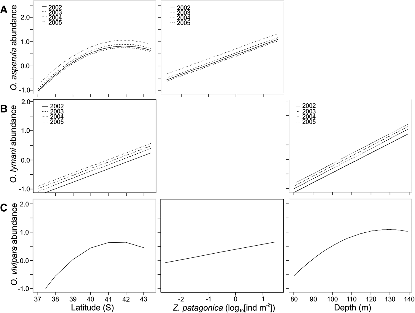
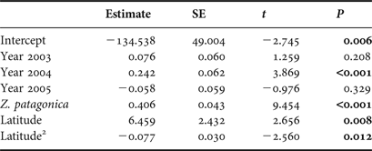
Ophiactis asperula abundance ranged from 0.009 to 337.89 ind m−2 per sample (mean abundance ± standard deviation = 18.83 ± 41.18 ind m−2, N = 514). This variability can be explained by latitude, Zygochlamys patagonica abundance and year (Table 1). The abundance of O. asperula showed a positive relationship with Zygochlamys patagonica (Figure 2A). Ophiactis asperula had a quadratic relationship with latitude; maximum abundances were registered between 41° and 42°S and in southern areas (Figure 2A). The abundance of O. asperula was significantly higher during 2004 (Figure 2A; Table 1).
(A) Ophiactis asperula: relationship between abundance (log10 [ind m−2 + 0.1]) and latitude and Zygochlamys patagonica abundance (log10 [ind m−2]), estimated from a generalized least squares (GLS) with normal distribution; (B) Ophiura (Ophiuroglypha) lymani: relationship between abundance (log10 [ind m−2 + 0.1]) and latitude and depth, estimated from a generalized linear model with normal distribution; (C) Ophiacantha vivipara: relationship between abundance (log10 [ind m−2]) and latitude, Zygochlamys patagonica abundance (log10 [ind m−2 + 0.1]) and depth (m), estimated from a GLS with normal distribution.

Results of generalized linear model among Ophiactis asperula abundance (log10 [x + 0.1]) and the variables selected by the Akaike information criterion. A spherical spatial correlation was used with range = 20 km and nugget = 0.3. The model explained 44% of the total variance. Z. patagonica = Zygochlamys patagonica abundance (log10 [ind m−2]). Significant relationships are in bold typeface.

Estimate, coefficient estimated; SE, standard error; t, observed value; P, significance level; 2, quadratic terms.
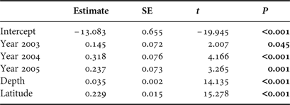
Ophiura (Ophiuroglypha) lymani was one of the less abundant species during the study period with a range abundance between 0.002 and 155.53 ind m−2 per sample and an estimated mean abundance of 3.76 ± 13.11 ind m−2 (N = 514). According to GLM results the variability within samples could be explained by latitude, depth and year (Table 2). Ophiura (Ophiuroglypha) lymani abundance increased with depth and latitude. The lowest abundance values were recorded in 2002 (Figure 2B).
Results of generalized linear model among Ophiura (Ophiuroglypha) lymani abundance (log10 [x + 0.1]) and the variables selected by the Akaike information criterion. The model explained 46.52% (F = 87.7, P < 0.01, N = 510) of the total variance. Significant relationships are in bold typeface.

Estimate, coefficient estimated; SE, standard error; t, observed value; P, significance level.
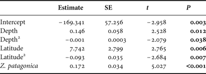
Ophiacantha vivipara had a mean abundance equal to 6.24 ± 11.03 ind m−2 in a variable range between 0.001 and 110.14 ind m−2 (N = 514). The GLS results are shown in Table 2; O. vivipara abundance showed a quadratic relationship with latitude and depth (Figure 2C; Table 3). The highest abundances were recorded at approximately 41° – 42°S and the lowest between 37°S and 38°S (Figure 2C). Ophiacantha vivipara also showed a positive relationship with Zygochlamys patagonica abundance (Figure 2C; Table 3). In regards to depth, the highest abundance values were recorded between 100 and 130 m (Figure 2C).
Results of generalized least squares among Ophiacantha vivipara abundance (log10[x + 0.1]) and the variables selected by the Akaike information criterion. A spherical spatial correlation was used with range = 20 km and nugget = 0.15. The model explained 55.81% of the total variance. Z. patagonica = Zygochlamys patagonica abundance (log10 [ind m−2]). Significant relationships are in bold typeface.

Estimate, coefficient estimated; SE, standard error; t, observed value; P, significance level; 2, quadratic terms.
As the relationship between abundance and depth was important for the three species, we plotted relative abundance of each station against depth (Figure 3). Although the three species coexist, we observed that Ophiactis asperula dominated at depths between 80 and 100 m with a conspicuous decrease in its abundance at depths more than 100 m (Figure 3). On the other hand, the abundance of Ophiacantha vivipara and Ophiura (Ophiuroplypha) lymani showed an increase at depths >100 m.
Ophiactis asperula, Ophiacantha vivipara and Ophiura lymani: relative abundance (%) versus depth (m).

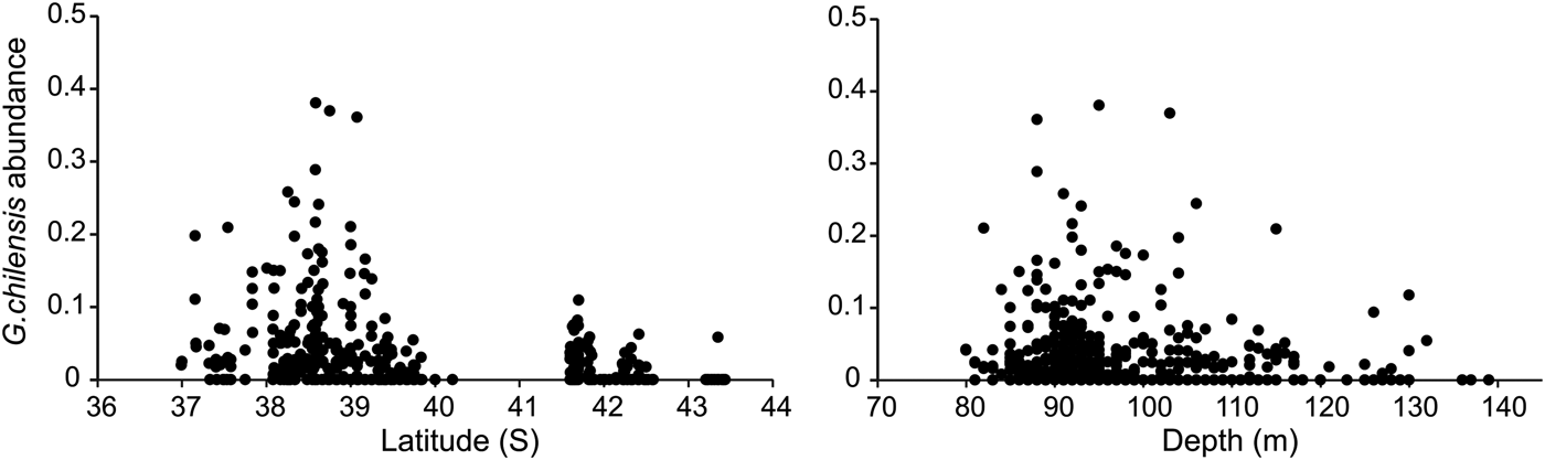
In the case of Gorgonocephalus chilensis no model fitted the data. Nevertheless, raw data showed more abundance of this species in northern and shallower areas (Figure 4).
Gorgonocephalus chilensis: abundance (ind m−2) in function of latitude (°S) and depth (m).

DISCUSSION
Ophiuroids are one of the dominant taxonomic groups on continental shelves, shelf-breaks and abyssal areas worldwide (Metaxas & Giffin, Reference Metaxas and Giffin2004; Chiantore et al., Reference Chiantore, Guideti, Cavallero, De Domenico, Albertelli and Cattaneo-Vetti2006; O'Hara, Reference O'Hara2007). Ophiactis asperula, Ophiacantha vivipara and Ophiura (Ophiuroplypha) lymani are the most abundant species in the benthic community associated with the shelf-break front (Bremec & Lasta, Reference Bremec and Lasta2002; Schejter et al., Reference Schejter, Bremec and Hernández2008; Escolar, Reference Escolar2010), and together with Zygochlamys patagonica, account for the major secondary production rates (Bremec et al., Reference Bremec, Brey, Lasta, Valero and Lucifora2000).
Ophiactis asperula, Ophiacantha vivipara and Ophiura (Ophiuroplypha) lymani were widely distributed in the study area. However, O. asperula was present over the full range of latitude and depths studied; this species dominated in terms of abundance. Ophiactis asperula and Ophiacantha vivipara showed a positive relationship with Zygochlamys patagonica abundance, early recognized as a characteristic of the epibenthic fauna associated with the shelf-break front in 1995, previous to the scallop fishery (Bremec & Lasta, Reference Bremec and Lasta2002). Ophiactis asperula, Ophiacantha vivipara and Z. patagonica are suspension feeders; therefore, high abundances of these species were recorded in those areas influenced by the high productivity of the shelf-break front (Acha et al., Reference Acha, Mianzan, Guerrero, Favero and Bava2004; Botto et al., Reference Botto, Bremec, Marecos, Schejter, Lasta and Iribarne2006; Mauna et al., Reference Mauna, Botto, Franco, Schwartz, Acha, Lasta and Iribarne2011).
The three species of ophiuroids showed a latitudinal distribution pattern increasing significantly southwards. The highest values of Ophiactis aperula and Ophiacantha vivipara were recorded between 41° and 43°S approximately, while the abundance of Ophiura (Ophiuroglypha) lymani increased beyond the study area; the location of the less abundant samples in this study coincided with the northern boundary of natural distribution of sub-Antarctic species (Bernasconi & D'Agostino, Reference Bernasconi and D'Agostino1977; Bartsch, Reference Bartsch1982; Barboza et al., Reference Barboza, Moura, Lanna, Oackes and Campos2011).
Bathymetric distribution patterns are commonly found in ophiuroids (Gage & Tyler, Reference Gage and Tyler1982; Summers & Nybakken, Reference Summers and Nybakken2000; Metaxas & Giffin, Reference Metaxas and Giffin2004) often related to food availability (Metaxas & Giffin, Reference Metaxas and Giffin2004; Booth et al., Reference Booth, Ruhl, Lovell, Bailey and Smith2008), oxygen concentration (Summers & Nybakken, Reference Summers and Nybakken2000), sediment type, salinity, temperature and currents (García et al., Reference García, Hsin-ming and Ohta2002; Manjón-Cabeza & Ramos, Reference Manjón-Cabeza and Ramos2003). In this study, the distribution of Ophiacantha vivipara and Ophiura (Ophiuroglypha) lymani was significantly influenced by depth, and although both species increased their abundance toward deeper areas, Ophiacantha vivipara reached its highest abundance values between 120 and 130 m.
The analysis of relative abundance per sample showed a depth segregation pattern among the three species: Ophiactis asperula was more abundant in samples collected between 80 and 100 m; Ophiacantha vivipara dominated in samples collected between 100 and 125 m; and Ophiura (Ophiuroplypha) lymani dominated in deeper samples (>125 m). Similar bathymetric distribution patterns were recorded for Ophiacantha vivipara and Ophiactis asperula before the Patagonian scallop fishery started (Roux et al., Reference Roux, Bastida and Bremec1993). Our results indicated that scallop fishing activities in the area did not affect the species distribution during the period 2002–2005.
As previously mentioned, niche separation in many species can be explained by different abiotic factors (Ventura & da Costa Fernandez, Reference Ventura and da Costa Fernandes1995; Gage et al., Reference Gage, Lamont, Kroeger, Paterson and Gonzalez Vecino2000; Tuya et al., Reference Tuya, Cisneros-Aguirre, Ortega-Borges and Haroum2007). It is known that substrates are rather homogeneous in the study area, with predominant soft sediments composed mainly of sand and variable shell content (Parker et al., Reference Parker, Paterlini, Violante and Boschi1997). Bottom temperatures range between 5° and 8°C with higher values in northern areas (~37.5°S) associated with the presence of the Brazilian Current over the slope (Bogazzi et al., Reference Bogazzi, Baldoni, Rivas, Martos, Reta, Orensanz, Lasta, Dell'Arcipetre and Werner2005). As the three ophiuroid species studied have omnivorous feeding habits, we propose that the different bathymetric patterns could represent a way of avoiding interspecific competition. Ophiactis species show diverse feeding strategies including deposit and suspension feeding (Warner, Reference Warner, Jangoux and Lawrence1982; Pearson & Gage, Reference Pearson and Gage1984; Hendler et al., Reference Hendler, Miller, Pawson and Kier1995). Ophiacantha species are suspension feeders, although organisms that reside on sediment surface were also recorded in their gut contents (Fell, Reference Fell1961; Pearson & Gage, Reference Pearson and Gage1984). Ophiacantha vivipara feeds on copepods and carrion in Antarctica (Fell, Reference Fell1961; Warner, Reference Warner, Jangoux and Lawrence1982; McClintock, Reference McClintock1994), while Ophiura (Ophiuroplypha) lymani feeds on detritus, sediment and crustaceans in southern Chile (Dahm, Reference Dahm1999). Clear depth segregation was observed although the bathymetric range of the three species overlaps (Bernasconi & D'Agostino, Reference Bernasconi and D'Agostino1977). This result could be supported by the feeding habits, since suspension feeder species like Ophiactis asperula and Ophiacantha vivipara were mainly recorded at lower depths influenced by the shelf-break front (Acha et al., Reference Acha, Mianzan, Guerrero, Favero and Bava2004; Bogazzi et al., Reference Bogazzi, Baldoni, Rivas, Martos, Reta, Orensanz, Lasta, Dell'Arcipetre and Werner2005; Mauna et al., Reference Mauna, Botto, Franco, Schwartz, Acha, Lasta and Iribarne2011). On the other hand, detritivorous species like Ophiura lymani would prefer deeper bottoms with higher contents of fine particles (Parker et al., Reference Parker, Paterlini, Violante and Boschi1997).
O'Hara et al. (Reference O'Hara, Rowden and Bax2011) showed that latitude and depth are two of the variables which contributed substantially to explain the distribution patterns of ophiuroids in the Indian, Pacific and Southern Oceans. According to O'Hara et al. (Reference O'Hara, Rowden and Bax2011), demographic and/or evolutionary processes may have an effect on ophiuroid distribution. In this case, the study area is recognized as transitional between the two biogeographical provinces in the Argentine Sea (Balech & Erlich, Reference Balech and Erlich2008). Ophiactis asperula is typical of the Argentine province, influenced by the northern Brazil Current, while Ophiacantha vivipara and Ophiura (Ophiuroglypha) lymani characterize the Magellan province, influenced by sub-Antarctic waters (Bernasconi & D'Agsotino, Reference Bernasconi and D'Agostino1977; Souto et al., Reference Souto, Escolar, Genzano and Bremec2011).
In conclusion, the most abundant ophiuroid species at the shelf break front, Ophiactis asperula, Ophiacantha vivipara and Ophiura (Ophiuroplypha) lymani, showed latitudinal and bathymetric distribution patterns explained partly by their feeding habits, a strategy that possibly helps to avoid interspecific competition. Studies on the biology and ecology of echinoderms are being developed to increase the knowledge about benthic invertebrates in the Argentinean continental shelf with particular emphasis on the productive shelf-break frontal system.
ACKNOWLEDGEMENTS
This work was supported by a doctoral scholarship from CONICET and comprises part of the doctoral dissertation of the leading author. This study was also partially supported by INIDEP; PICT 2007-02200; and the Inter-American Institute for Global Change Research (IAI) CRN 2076 with funding from the US National Science Foundation (Grant GEO-0452325). We thank technicians and colleagues at INIDEP who helped us during general sampling procedures. Special thanks to Dr F. Cortés and Dr R. Di Mauro for their advice and comments on this manuscript. This is INIDEP Contribution No. 1843.