3.1. Maxwell stress tensor

We first consider the Maxwell stress tensor in the context of electromagnetism. The Maxwell stress tensor, typically defined as

(3.1) \begin{equation} {T_{\textit{ij}}} = {\varepsilon _0}\left ( {{E_{i}}\kern-1pt{E_{\!j}} - \frac {1}{2}{E_k}{E_k}{\delta _{\textit{ij}}}} \right ) + \frac {1}{{{\mu _0}}}\left ( {{B_i}\kern-1pt{B_{\!j}} - \frac {1}{2}{B_k}{B_k}{\delta _{\textit{ij}}}} \right )\!, \end{equation}

describes the distribution of electromagnetic momentum and forces within a medium. Here, $E_i$ and $B_i$ are the components of the electric and magnetic fields, respectively, $\varepsilon _0$ is the vacuum permittivity and $\mu _0$ is the vacuum permeability.

A three-dimensional cube with sinusoidally varying fields is used to evaluate the behaviour governed by (3.1). The electric field is given by

(3.2) \begin{equation} E(x,y,z) = [{E_0}\sin (\pi\kern-1pt x),{E_0}\cos (\pi\kern-1pt y),{E_0}\sin (\pi\kern-1pt z)], \end{equation}

and the magnetic field is given by

(3.3) \begin{equation} B(x,y,z) = [{B_0}\cos (\pi\kern-1pt x),{B_0}\sin (\pi\kern-1pt y),{B_0}\cos (\pi\kern-1pt z)], \end{equation}

where ${E_0} = {10^6}{\text{ V m}^{-1}}$ and ${B_0} = {10^{ - 3}}{\text{ T}}$ are fixed amplitudes. To construct the dataset, 150 spatial points are randomly sampled within the cube ( $- 1\leqslant x,y,z\leqslant 1$ ), and the corresponding Maxwell stress tensor is computed analytically using (3.1). The schematic diagram of this case is shown in figure 5(a).

Figure 5.

(a) Schematic diagram of the electric field, the magnetic field and sampled points. For clarity of illustration, only the vectors along the guiding dashed line are shown. (b) Trend lines of the electromagnetic field magnitude at the points along the guiding line in (a) before and after adding $5\,\%$ Gaussian noise. The solid line represents the ideal setting, and the dashed line represents the real situation.

In this case, the target variable is defined as $T_{\textit{ij}}$ . For tensors, the candidate function library and the candidate terminal library are defined as $\{ + , - , \boldsymbol{\cdot },{\text{p}}\}$ and $\{ {E_{i}}\kern-1pt{E_{\!j}},{B_i}\kern-1pt{B_{\!j}},{\delta _{\textit{ij}}}\}$ , respectively, while for scalars, the candidate function library and the candidate terminal library are defined as $\{ + , - , \times , \div \}$ and $\{ E_{i}E_{i},B_{i}B_{i},{\varepsilon _0},{\mu_0}\}$ . The candidate terminal libraries of different tests are exactly the same.

To highlight the contribution of TLR to improving coefficient optimization efficiency, we conduct comparative experiments under three configurations: (i) using only RNC, (ii) using only TLR and (iii) combining TLR with RNC. When TLR is not employed, RNC must be introduced into the scalar candidate terminal library to form numerical constants in expressions. These RNC are randomly sampled floating-point numbers within the range $[-10,10]$ . 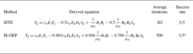The hyperparameter settings for the comparative experiments are basically the same, except that additional genetic operations need to be performed on RNC when they are introduced (see Appendix A). Detailed parameter settings for the SITE algorithm, such as the maximum number of evolutionary generations and the number of host individuals, are provided in Appendix B. The derived equations for this test, along with the number of iterations and the central processing unit (CPU) runtime (measured on a system equipped with a 13th Gen Intel Core i9-13900K CPU at 3.00 GHz, 32 GB RAM and running a 64-bit operating system), are summarized in table 1.

Table 1.

Performance comparison of SITE using different coefficient optimization configurations.

Table 2.

Performance comparison between SITE and M-GEP.

*Note that one of the three success runs does not explicitly include $\varepsilon _0$ and $\mu _0$ , but the approximate coefficients were numerically consistent with their values. Considering that M-GEP uses non-dimensionalization to preprocess the data instead of using DHCs to constrain the evolutionary process, we think this equation with low discrepancy can also be regarded as successfully identifying the target equation.

It can be seen from table 1 that regardless of whether TLR is used, SITE is capable of discovering complex tensor equations from the data. However, the success rate shows a clear difference across configurations. Without TLR, the framework fails to identify a completely correct equation in all five runs, yielding a success rate of 0 $/$ 5 even after the maximum number of evolutionary generations. Specifically, the coefficients of the discovered terms are incorrect and the combination of ${B_k}{B_k}{\delta _{\textit{ij}}}$ and $({1}/{{{\mu _0}}})$ is not identified. This is because optimization based on RNC relies only on completely random mutations to alter the numerical coefficients in the expression. In contrast, when TLR is used, SITE consistently identifies the exact target equation in all five runs, achieving a success rate of $5\kern-0.5pt/\kern-0.5pt5$ and substantially reducing the number of iterations required. It is evident that TLR substantially improves the efficiency and accuracy of tensor equation identification. Moreover, we tested a third configuration where RNC are removed and only TLR is used. The SITE achieves the same accuracy within 182 iterations on average, demonstrating that TLR alone is sufficient to achieve both high accuracy without relying on RNC. Since the mingling of RNC with symbolic terminals sometimes may hinder the generation of concise expressions, all cases in this article use only TLR to optimize coefficients unless otherwise specified.

To further benchmark SITE against the state-of-the-art method, we compare it with the latest EVE-3 implementation of M-GEP using the same dataset as above. As shown in table 2, M-GEP achieves a success rate of $3\kern-0.5pt/\kern-0.5pt5$ with an average of 500 iterations. In one of these successful runs, the discovered equation does not explicitly include $\varepsilon _0$ and $\mu _0$ , yet the approximate coefficients are numerically consistent with their physical values. Since M-GEP relies on non-dimensionalization for preprocessing instead of enforcing dimensional homogeneity as in SITE, such cases are still regarded as successful identifications. In contrast, SITE consistently identifies the exact Maxwell stress tensor equation in all five runs, with an average of only 182 iterations. These results highlight that SITE not only ensures higher reliability (success rate $5\kern-0.5pt/\kern-0.5pt5$ versus $3\kern-0.5pt/\kern-0.5pt5$ for M-GEP), but also achieves better efficiency.

To evaluate the robustness of SITE to Gaussian noise, we test its performance under three noise levels: $5\,\%$ , $10\,\%$ and $20\,\%$ . Specifically, as illustrated as figure 5(b), Gaussian noise is first added to the electric and magnetic field strengths to generate perturbed physical quantities. Then, Maxwell stress tensors are computed from these noisy fields and further perturbed by Gaussian noise of the same level. These noisy data are used for the subsequent tests. Here, we use both RNC and TLR here to get results quickly.

The derived equations with different levels of noise are listed in table 3. The error in the table is defined as the average relative error of the identified non-zero coefficients with respect to the ground truth. When Gaussian noise is added, the coefficients in the equation identified by SITE deviate increasingly from the ground truth as the noise level increases, and the error grows almost linearly with the noise level. Even with up to $20\,\%$ Gaussian noise, SITE still successfully identifies the complete structure of the expression, although there are some deviations in the coefficients. This proves that the framework has great robustness against artificial noise.

Table 3.

Equations identified by SITE under different levels of Gaussian noise ( $5\,\%$ , $10\,\%$ and $20\,\%$ ).

3.2. Reynolds-stress transport equation

In many physical systems, the evolution of tensors is governed by time-dependent differential equations. To evaluate the capability of SITE to identify such dynamic tensor equations, we consider the following general form of a time-dependent tensor evolution equation:

(3.4) \begin{equation} \frac {{{\rm d}{T_{\textit{ij}}}}}{{{\rm d}t}} = F(\{\boldsymbol{a}_{\textit{ij}}\},\{\boldsymbol{x}\}) \end{equation}

where $T_{\textit{ij}}$ is a second-order tensor, while $\boldsymbol{a}_{\textit{ij}}$ and $\boldsymbol{x}$ represent a group of second-order tensors and scalars, respectively. Note that when spatial derivatives of the tensor $T_{\textit{ij}}$ appear on the right-hand side of the equation, it becomes a PDE.

To generate data for the discovery of this kind of tensor equation, simulations are performed for three-dimensional compressible decaying homogeneous isotropic turbulence. The simulation employs a uniform grid of $32\times 32\times 32$ cells, a backward Euler time advancement scheme with a time step of ${1 \times {10}^{-7}}\,\textrm {s}$ , and a total simulation time of ${4 \times {10}^{-6}}\,\textrm {s}$ . Argon gas is used as the working fluid, with initial conditions of ${273.15}\,\textrm {K}$ temperature, 100 000 Pa pressure and zero mean velocity. The initial turbulent kinetic energy is set to ${4265.9}\,{{\textrm {m}}^2\, {\textrm {s}}^{-2}}$ , corresponding to an initial turbulent Mach number of 0.3. The flow is initialized following the procedure of Ma et al. (Reference Ma, Yang, Chen, Feng, Cui and Zhang2024a ), and computed using the open-source solver OpenFOAM with periodic boundary conditions (Jasak, Jemcov & Tukovic Reference Jasak, Jemcov and Tukovic2007) In our simulation, a modelled Reynolds stress transport equation is solved in OpenFOAM using the Launder–Reece–Rodi model (Launder, Reece & Rodi Reference Launder, Reece and Rodi1975). Therefore, the target governing equation takes the form

(3.5) \begin{equation} \frac {{\rm D}(\rho\kern-1pt R_{\textit{ij}})}{{\rm D}t} = \rho\kern-1pt P_{\textit{ij}} - 1.8\frac {\varepsilon }{k}\rho\kern-1pt R_{\textit{ij}}^* - 0.6\rho\kern-1pt P_{\textit{ij}}^* - \frac {2}{3}\rho \varepsilon \delta _{\textit{ij}} + D_{\textit{ij}}, \end{equation}

where the Reynolds stress is defined as $R_{\textit{ij}}=\overline {u_i' u_{\!j}'}$ , $\rho$ is the density, $k$ the turbulent kinetic energy and $\varepsilon$ the dissipation rate. Here, $(\boldsymbol{\cdot })^*$ denotes the trace-free part of a tensor and ${\rm D}(\boldsymbol{\cdot })/{\rm D}t$ the material derivative. In this formulation, the production term $P_{\textit{ij}}$ is computed explicitly from the resolved mean flow, while the remaining terms are modelled slow and rapid pressure-strain correlations, dissipation and diffusion terms, respectively. All tensors and scalars in (3.5) are directly computed and output by the solver.

In the previous case, we have evaluated the robustness of the framework under Gaussian noise. In this case, we further conduct more challenging noise robustness tests – all the physical quantities used are derived from the computational fluid dynamics simulation results. Specifically, two representative datasets are constructed: (i) a clean dataset, where the target material derivative is assembled directly from the right-hand side of (3.5); and (ii) a noisy dataset, where the target tensor is taken from solver outputs and thus contains discretization errors. Both datasets consist of 200 randomly sampled spatiotemporal points, and remain fixed across independent SITE runs.

The target variable is defined as $({{\rm D}(\rho R_{\textit{ij}})}/{{\rm D}t})$ . For tensors, the candidate function library and the candidate terminal library are defined as $\{ + , - , \boldsymbol{\cdot },(\boldsymbol{\cdot })^*,{\text{p}}\}$ and $\{P_{\textit{ij}}, R_{\textit{ij}}, D_{\textit{ij}}, \delta _{\textit{ij}} \}$ , respectively, while for scalars, the candidate function library and the candidate terminal library are defined as $\{ + , - , \times , \div \}$ and $\{\rho , k, \varepsilon \}$ .

As shown in table 4, SITE consistently recovers the correct equation from the clean dataset in all five independent runs, without any coefficient errors. For the noisy dataset, four out of five runs yield the correct equation structure with comparable accuracy. In the unsuccessful run, an additional traceless diffusion term $D_{\textit{ij}}^*$ appears with a small coefficient of $0.03$ , which is one order of magnitude lower than those of the dominant terms. This spurious term is attributed to data noise rather than physical relevance, indicating that while noise may occasionally induce weak redundant terms, the main physical effects are still robustly captured.

Table 4.

Equations identified by SITE from clean dataset and noisy dataset.

Beyond the above baseline results, we further challenge SITE on the clean dataset to test its expressive capability. Methodologically, SITE’s candidate tensor function library is designed to be both expressive and flexible, having the ability to contain operators such as trace-free and transpose. To intensify the test, we replace the turbulent production term $P_{\textit{ij}}$ with the raw velocity gradient tensor $\partial u_i/\partial x_{\!j}$ , where

(3.6) \begin{equation} P_{\textit{ij}} = - R_{\textit{ij}}\frac {\partial u_{\!j}}{\partial x_k} - R_{jk}\frac {\partial u_i}{\partial x_k}. \end{equation}

In this setting, SITE is required not only to recover all terms in the complete Reynolds-stress transport equation, but also to reconstruct $P_{\textit{ij}}$ from its lower-level components. Remarkably, the exact target equation was successfully identified within 1000 generations, highlighting the strong expressive capability of SITE.

For this problem, a direct comparison with M-GEP is not feasible. The reason is that M-GEP requires all necessary tensors to be explicitly prespecified in advance – for example, the trace-free tensors must be provided beforehand – whereas in our setting we allow the trace-free operator itself to be included as a candidate symbol in the function library, letting SITE autonomously select and construct the appropriate symbolic structures.

Additionally, we conduct an ablation study on the role of DHC using the clean dataset here. Table 5 summarizes the results for SITE with and without DHC. With DHC enabled, SITE consistently identifies the correct target equation in all five independent runs. In contrast, under our strict success criterion, the version without DHC produces the exact target equation only once out of five runs; although in the remaining runs it still achieves very low loss values by leveraging TLR, the resulting equations include spurious terms such as $\delta _{\textit{ij}}$ and $((({{\rho {\varepsilon ^2}}})/{{2k\varepsilon + k^2}})R_{\textit{ij}})$ , which are physically uninterpretable. In terms of efficiency, introducing DHC significantly reduces the number of non-physical candidate combinations that require evaluation, leading to fewer iterations per run and a markedly lower CPU runtime. These results confirm that DHC not only enhances the physical interpretability of the identified equations but also reduces the effective search space, thereby improving computational efficiency.

Table 5.

Performance comparison of SITE with or without DHC on the clean dataset.

4.1. Data generation and preprocessing

In this section, we employ the DSMC method (Bird Reference Bird1994) to generate flow field data, following the approach in Zhang & Ma (Reference Zhang and Ma2020) and Ma et al. (Reference Ma, Zhang, Feng, Xing and Wen2024b ). Since the aim of this section is to discover tensor macroscopic governing equations of fluid dynamics, it is crucial that the data be independent of macroscopic modelling assumptions. The DSMC method fulfils this requirement by simulating particle dynamics without reliance on predefined continuum-level equations such as the Navier–Stokes equations. In DSMC, each simulation molecule statistically represents a large number of real molecules. From these molecular-level dynamics, macroscopic physical quantities are obtained via statistical averaging. For instance, the velocity field ( $v_i$ ) and the pressure tensor field ( $p_{\textit{ij}}$ ) are computed as

(4.1) \begin{equation} {v_i} = \frac {1}{{{N_{\textit{p}}}}}\sum \limits _{{\textit{cell}}} {{c_i}} ,\quad {p_{\textit{ij}}} = \frac {{mF}}{{{V_{{\textit{cell}}}}}}\left ( {\sum \limits _{{\textit{cell}}} {{c_i}}\kern-1pt{c_{\!j}} - {N_{\textit{p}}}{v_i}\kern-1pt{v_{\!j}}} \right )\!, \end{equation}

where $N_{\!p}$ is the number of simulation molecules in the sampling cell, $c_i$ is the velocity of the $i$ th particle, $m$ is the molecular mass and $F$ is the simulation ratio in DSMC. With the data generated from DSMC, we can construct a mapping from spatial coordinates to various macroscopic variables. As illustrated in figure 1(a), at each given data point $(x,y)$ , we associate corresponding physical quantities such as density $\rho (x,y)$ , horizontal velocity $u(x,y)$ and vertical velocity $v(x,y)$ .

In our study, two primary sources of noise affect the accuracy of equation discovery. One is the numerical noise arising from the computation of spatial gradients, and the other is the statistical noise inherent in particle-based methods such as DSMC. To mitigate the first type of noise, we apply the neural-network-based automatic differentiation technique to calculate gradients of physical variables. Specifically, an artificial neural network is trained to map spatial coordinates to macroscopic variables, and gradients of arbitrary order are obtained by backpropagating through the network. This allows accurate evaluation of spatial derivatives at any point in the domain. As for the statistical noise introduced by particle simulation, we can quantitatively estimate how the statistical error changes with the number of statistical samples (Hadjiconstantinou et al. Reference Hadjiconstantinou, Garcia, Bazant and He2003) with

(4.2) \begin{equation} {E_{\!Q}} = \frac {1}{{\sqrt {{N_0}M} }}\frac {{\sqrt {\left \langle {{Q^2}} \right \rangle } }}{{\left | {\left \langle Q \right \rangle } \right |}}, \end{equation}

where $E_{\!Q}$ represents the statistical error of quantity $Q$ , $\left \langle {{\boldsymbol{\cdot }}} \right \rangle$ means the statistical mean value, $N_0$ is the number of particles in a statistical cell and $M$ is the number of independent samples. In our study, we set the ${N_0}M$ of our simulation to $4 \times {10^9}$ , which means the statistical error of $p_{\textit{ij}}$ is around $10^{ - 5}$ . An error of this magnitude is acceptable for our experiments.

We simulate lid-driven cavity flows using the DSMC method described above. The simulated domain is a square cavity with a side length of $L = {1}\,\textrm {m}$ , filled with argon gas. All four walls maintain at a constant temperature of 273.15 K. The bottom, left- and right-hand walls are stationary, while the top wall (lid) moves horizontally at a constant speed. The number of grids is set to $400 \times 400$ . Each grid cell provides DSMC statistical outputs of the horizontal and vertical velocities, the four components of pressure tensor, the temperature and the static pressure. Two flow conditions are considered by setting the lid velocity to different values. In the first case, the lid speed is set to 50 m s^–1, corresponding to a low-speed, nearly incompressible flow. In the second case, the lid velocity is increased to 337 m s^–1, resulting in a transonic, compressible flow. The DSMC simulations employ the variable hard sphere model, in which the dynamic viscosity varies with temperature according to

(4.3) \begin{equation} \mu = {\mu _{{\textit{ref}}}}{\left ( {\frac {T}{{{T_{{\textit{ref}}}}}}} \right )^\omega } \end{equation}

where ${\mu _{{\textit{ref}}}}\,=\,{2.117\times {10}^{-5}}{{\textrm {kg}}(\textrm {m} \boldsymbol{\, }\textrm {s})^{-1}}$ denotes the reference viscosity coefficient, ${T_{{\textit{ref}}}} = {273.15}\,\textrm {K}$ denotes the reference temperature, and $\omega = 0.81$ denotes the viscosity exponent. The global Knudsen number in both cases is fixed at $K{\kern-1pt}n = 0.005$ .

To enable the computation of velocity gradients, we trained neural networks to learn the mapping from spatial coordinates to the two velocity components within the flow field. Specifically, we used all $400\times 400$ data points from the computational domain as the training set. The mapping was modelled using a fully connected feedforward neural network comprising eight hidden layers, each with 60 neurons and tanh activation functions. The training process was carried out in two stages. First, we used the Adam optimizer (Kingma & Ba Reference Kingma and Ba2017) for $20\,000$ iterations to achieve a reasonable initial solution. Then, the optimization was refined using the L-BFGS-B (Byrd et al. Reference Byrd, Lu, Nocedal and Zhu1995) optimization until convergence. This hybrid optimization strategy ensures both stability and precision in capturing smooth and differentiable velocity fields suitable for gradient extraction via automatic differentiation.

4.2. Constitutive equation discovery under different flow conditions

With the DSMC datasets described in § 4.1, we now apply SITE to identify the constitutive equations under both flow conditions.

In constructing the candidate function library, we introduced a set of basic tensor and scalar operators. As for the candidate terminal library, special consideration was given to the physical relevance of constitutive modelling. Since constitutive relation of pressure tensor reflects the transport of momentum in the flow field – and such transport is primarily driven by velocity gradients – we included physical quantities related to the velocity gradient tensor. The velocity gradient tensor ${D_{\textit{ij}}} = \partial {u_i}/\partial {x_{\!j}}$ can be decomposed into a symmetric and an antisymmetric part, given as

(4.4) \begin{equation} {D_{\textit{ij}}} = {S_{\textit{ij}}} + {\varOmega _{\textit{ij}}}, \end{equation}

where ${S_{\textit{ij}}} = ({1}/{2}) ( {{D_{\textit{ij}}} + {D_{ji}}} )$ is the symmetric strain-rate tensor, and ${\varOmega _{\textit{ij}}} = ({1}/{2}) ( {{D_{\textit{ij}}} - {D_{ji}}} )$ is the antisymmetric rotation-rate tensor. In both cases, the target variable is defined as $p_{\textit{ij}}$ . For tensors, the candidate function library is defined as $\{ + , - , \boldsymbol{\cdot },{\text{p}}\}$ and $\{ {S_{\textit{ij}}},{\delta _{\textit{ij}}}\}$ , respectively, while for scalars, the candidate function library and the candidate terminal library are defined as $\{ + , - , \times , \div \}$ and $\{ {D_{\textit{ii}}},p,\mu \}$ . For a detailed description of the construction of the candidate term library used in this study, please refer to Appendix C.

The last step before applying SITE is subsampling the dataset. To mitigate the influence of numerical noise when computing gradients near the boundaries, we restricted the sampling region to the central portion of the domain – specifically, the $20\,\%$ to $80\,\%$ range along both spatial directions. From this subregion, 200 data points were randomly selected and used for symbolic regression and equation discovery. Figure 6 illustrates the distribution of velocity magnitude (defined as $\sqrt {{u^2} + {v^2}}$ ) across the domain in the compressible cavity flow case, along with a schematic representation of the sampled data points used for training. This selection strategy ensures that the discovered equations are based on high-quality gradient information. We exclude regions where boundary effects or numerical errors may distort the constitutive relation, while still retaining a sufficiently large and diverse dataset. It has been verified that the dominant terms identified by SITE are insensitive to the precise cutoff as long as noisy near-wall data are excluded. This strategy is a practical guideline. For other problems, a similar strategy can be adopted by first assessing the reliability of gradient information and then subsampling a central region large enough to capture the dominant physical effects.

For reference, the complete Newtonian constitutive relation is given by

(4.5) \begin{equation} {p_{\textit{ij}}} = - 2\mu {S_{\textit{ij}}} + \frac {2}{3}\mu {D_{\textit{kk}}}{\delta _{\textit{ij}}} + p{\delta _{\textit{ij}}}. \end{equation}

This form can be derived under the continuum hypothesis. The first term is the shear stress term, which arises from the internal friction caused by the relative sliding (shear deformation) between fluid layers, corresponding to the anisotropic behaviour of shear stress. The second term is the compressible term, accounting for the viscous resistance generated during volumetric changes. This term is typically negligible in incompressible flows where the velocity divergence is close to zero. The third term is the static pressure term, representing the isotropic compressive stress imposed by the thermodynamic pressure, which is independent of the flow state. In our DSMC simulations, the macroscopic constitutive relation is not imposed a priori. Since the global Knudsen number is small in this case, it is reasonable to expect that the effective constitutive relation should be close to Newtonian, but this does not imply that the ‘ground truth’ is (4.5). This is fundamentally different from a benchmark case. In this section, the success of equation identification is not judged by comparison with the Newtonian constitutive form, but rather by the objective metric of test error (refer to Appendix D for details). The reported identified equations are constructed from the results of five independent runs. Specifically, we only keep the common terms that appear across these runs, and average their coefficients to form the reported equation.

As shown in table 6, we summarize the constitutive equations discovered in the two test cases. The identified constitutive equations vary with the lid velocity, reflecting the features of different flow conditions. At the lower velocity, the discovered relation contains only the shear stress term and the static pressure term, which is consistent with the expectation that compressibility effects are weak when the flow remains nearly incompressible. At the higher velocity, an additional term proportional to $\mu D_{\textit{kk}}\delta _{\textit{ij}}$ emerges. This term accounts for the resistance associated with compressibility and indicates that the framework successfully detects flow-dependent physical contributions.

Table 6.

Identified equations of cavity flow.

Figure 6.

Distribution of velocity magnitude in the compressible cavity flow case and the spatial locations of sampled data points used for SITE.

It is also noteworthy that the coefficients identified by SITE exhibit slight deviations from those in the classical Newtonian constitutive model. These discrepancies may be attributed to the fact that the simulated flows are not strictly within the continuum regime. Locally, some features of slip flow may appear. Based on the Knudsen number ( $\textit{Kn}$ ), flow regimes can be classified into continuum ( $\textit{Kn} \lt 0.001$ ), slip ( $0.001 \lt \textit{Kn} \lt 0.1$ ), transition ( $0.1 \lt \textit{Kn} \lt 10$ ) and free-molecular ( $\textit{Kn} \gt 10$ ) regimes (Reese, Gallis & Lockerby Reference Reese, Gallis and Lockerby2003). Since molecular simulations are computationally expensive in the fully continuum regime, we selected a global $\textit{Kn} = 0.005$ to balance accuracy and efficiency. Consequently, local deviations from continuum assumptions may still exist.

4.3. Discussion on magnitude disparities

A key challenge in data-driven modelling lies in the simultaneous identification of terms with vastly different magnitudes from noisy data. In our compressible cavity flow case, this issue becomes particularly evident. The off-diagonal components, $p_{xy}$ and $p_{yx}$ , are governed solely by shear deformation and is thus dominated by the symmetric part of the velocity gradient tensor. Consequently, identifying $S _{\textit{ij}}$ -related terms in this case is relatively straightforward. In contrast, the diagonal components of the pressure tensor tensor are composed of contributions from shear stress term, compressible term (linked to $\nabla \boldsymbol{\cdot} \boldsymbol{u}$ ) and static pressure $p$ . Among these, the compressible term typically has the smallest magnitude in the current case (see figure 7).

Figure 7.

Distributions of the constitutive terms in the xx-direction of the compressible cavity flow case. (a) Pressure tensor component ${p _{\textit{xx}}}$ , (b) static pressure $p$ ; these two quantities have similar magnitudes and are shown with a shared colour scale. (c) Shear viscosity contribution $\mu {S_{\textit{xx}}}$ , (d) compressible contribution $\mu (\boldsymbol{\nabla} \boldsymbol{\cdot} \boldsymbol{u})$ ; these two quantities have similar magnitudes and are shown with a shared colour scale. The average absolute values over the entire domain are indicated in red text within each panel. Quantitatively, $\mu (\boldsymbol{\nabla} \boldsymbol{\cdot} \boldsymbol{u})$ is roughly four orders of magnitude smaller than the dominant stress terms, posing a significant challenge for data-driven discovery.

In this case, the problem can be simplified by subtracting the pressure to isolate the trace-free parts $\sigma_{\textit{ij}} = p_{\textit{ij}} - p \delta_{\textit{ij}}$ . However, to rigorously evaluate whether SITE can discover small-magnitude terms amid much larger dominant contributions, we deliberately choose to identify the complete constitutive relation of $p_{\textit{ij}}$ . The results in § 4.2 have shown that SITE is capable of reliably identifying the compressible term under such challenging conditions. This highlights the framework’s robustness to large disparities in variable magnitudes.

This robustness arises from SITE’s design principles that explicitly address magnitude disparities without distorting physical significance. Compared with sparse regression-based methods which relies on standardized feature spaces and regularization to suppress terms with small numerical contributions, SITE operates directly in the native physical scale and preserves candidate terms through evolutionary mechanisms. Subexpressions such as $\mu D_{\textit{ii}}$ are retained and re-evaluated across generations, even if their immediate numerical contribution is minimal.

In addition to the overall magnitude disparity between different terms, another challenge specific to tensor equation identification lies in the magnitude disparity of different components within a single tensor. Unlike scalar regression tasks where each feature corresponds to a single physical quantity, tensor modelling requires treating entire tensor structures as regression targets. However, the magnitudes of different components within a tensor (e.g. the diagonal and off-diagonal terms in $p_{\textit{ij}}$ ) can vary significantly. This disparity can bias the learning process if not properly addressed. In SITE, this issue is mitigated by the design of optimization objective. The loss function (2.6) incorporates a normalization scheme that rescales each component individually. This ensures that each tensor component contributes equally to the total loss, regardless of its absolute magnitude, thereby improving the robustness of coefficient identification.