2 The model

The hydrostatic Boussinesq equations on the ‘ $f$ -plane’ are

where $\boldsymbol{v}=(u,v)$ and $w$ are the horizontal and vertical velocities respectively, $b$ is the buoyancy, $p$ is the pressure, $\boldsymbol{f}=f\hat{\boldsymbol{z}}$ is the constant rotation rate, $N$ is the buoyancy frequency and $\unicode[STIX]{x1D735}=(\unicode[STIX]{x2202}_{x},\unicode[STIX]{x2202}_{y})$ .

At oceanic mesoscales, the barotropic and the first baroclinic mode contain most of the geostrophically balanced energy, as inferred from oceanic observations (Wunsch Reference Wunsch1997), theoretical estimates (Fu & Flierl Reference Fu and Flierl1980) and idealized numerical simulations (Smith & Vallis Reference Smith and Vallis2001). Additionally, satellite altimetry data show that the mode-1 internal tide, corresponding to the first baroclinic mode inertia–gravity wave, contains a large fraction of internal tide energy (see for example Ray & Zaron Reference Ray and Zaron2016 and Zhao et al. Reference Zhao, Alford, Girton, Rainville and Simmons2016). Motivated by these observations that indicate dominant wave and balanced energies in the lowest vertical modes, we truncate the primitive equations to the barotropic and the first baroclinic mode. We assume constant buoyancy frequency $N$ and expand all variables in terms of the barotropic and the first baroclinic mode as:

where $\boldsymbol{x}=(x,y)$ and $H$ is the ocean depth. Using above expansion and projecting (2.1) on the two vertical modes gives us

Reduced models of the form (2.3) obtained by truncating the three-dimensional equations to two vertical modes have been popular in different fields of study. For instance, Frierson, Majda & Pauluis (Reference Frierson, Majda and Pauluis2004), Stechmann & Majda (Reference Stechmann and Majda2006) and Pauluis, Frierson & Majda (Reference Pauluis, Frierson and Majda2008) used such two-vertical-mode systems to examine tropical–extratropical interactions in the atmosphere. On a different route, Benavides & Alexakis (Reference Benavides and Alexakis2017) recently examined the turbulent dynamics of non-rotating thin fluid layers using a similar two-vertical-mode truncated model. While truncated models, such as (2.3) and those mentioned above, undoubtedly miss key small-scale features generated by higher vertical modes, such idealized and tractable models offer easier insight into the various nonlinear interactions involved in generating the complex flow dynamics, in comparison to more complicated fully three-dimensional models. The reader is referred to the discussion in § 4 for a detailed description of the potential differences we anticipate in a fully three-dimensional investigation.

Returning to our two-vertical-mode truncated equations, we note that in (2.3a ), spatially homogeneous inertial oscillation corresponding to the zeroth Fourier mode, with the time derivative balancing the Coriolis term, is the only fast oscillating linear mode. Numerically integrating the above system in the various regimes discussed in this paper, we found this mode to be energetically insignificant and dynamically passive in terms of its effect on other modes. Therefore we take one more step to simplify our model by ignoring the spatially homogeneous inertial oscillation. We take the curl of (2.3a ) and define $\unicode[STIX]{x1D701}_{T}=\unicode[STIX]{x1D735}\times \boldsymbol{v}_{T}$ to replace (2.3a ) and (2.3b ) by

Equations (2.4), (2.3c ) and (2.3d ) constitute our model for the present work. We non-dimensionalize all variables as

where $L_{D}=NH/\unicode[STIX]{x03C0}f$ is the first deformation scale. In the above scaling, we used a single velocity scale, $U$ , to non-dimensionalize both barotropic and baroclinic velocity components. From the point of view of the freely evolving turbulent simulations that we discus below, $U$ may be considered to be the largest velocity magnitude present in the system at $t=0$ . Using (2.5) in (2.4), (2.3c ) and (2.3d ) gives us our final set of equations

where $Ro=U/fL_{D}$ is the Rossby number. Note that since we chose our length scale, $L$ , to be the deformation scale, the Burger number, $Bu=(L_{D}/L)^{2}$ , a second non-dimensional parameter, does not explicitly appear in the above equations.

Throughout this paper, we use subscripts $T$ and $C$ to represent the barotropic and the baroclinic fields respectively. Consequently in (2.6), $\unicode[STIX]{x1D701}_{T}$ is the barotropic vorticity corresponding to the divergence free barotropic velocity field $\boldsymbol{v}_{T}$ , whereas $\boldsymbol{v}_{C}$ and $p_{C}$ refer to baroclinic velocity and pressure respectively. Our focus here is on the mesoscale regime characterized by small Rossby number, $Ro=U/fL_{D}\ll 1$ . We are therefore set in a parameter regime where both the wave field and the balanced flow have an $O(1)$ Burger number, and in this sense this case differs from several previous investigations that have examined interactions between asymptotically small Burger number NIWs and $O(1)$ Burger number balanced flows.

3 Numerical experiments

To investigate the geophysical turbulence phenomenology in different cases, we numerically integrated (2.6) in the small Rossby number regime by setting $Ro=0.1$ . For each experiment, equation (2.6) was integrated up to $t=30\,000$ on a $[0,2\unicode[STIX]{x03C0}]^{2}$ doubly periodic domain with a dealiased pseudospectral code. All our results presented below were based on simulations with $384^{2}$ grid points, which corresponded to $128^{2}$ active Fourier modes after two-thirds dealiasing (or an equivalent resolution of $256^{2}$ ). Selected simulations were run at double the resolution to ensure that the results discussed below were unaffected by our resolution. Hyperdiffusion terms of the form $\unicode[STIX]{x1D708}\unicode[STIX]{x1D6E5}^{8}\unicode[STIX]{x1D701}_{T}$ , $\unicode[STIX]{x1D708}\unicode[STIX]{x1D6E5}^{8}\boldsymbol{v}_{C}$ and $\unicode[STIX]{x1D708}\unicode[STIX]{x1D6E5}^{8}p_{C}$ were added to equations (2.6) to dissipate small-scale features and represent the only mechanism by which total energy is lost. Use of a high-order dissipation operator ( $\unicode[STIX]{x1D708}\unicode[STIX]{x1D6E5}^{8}$ , similar to Farge & Sadourny (Reference Farge and Sadourny1989), Maltrud & Vallis (Reference Maltrud and Vallis1993) and Musacchio & Boffetta (Reference Musacchio and Boffetta2019) for example), allowed us to have an extended range of inviscid scales for the chosen spatial resolution. The dissipation wavenumber, $k_{d}$ , corresponding to the $\unicode[STIX]{x1D708}\unicode[STIX]{x1D6E5}^{n}$ hyperdissipation operator is given by (see for example Spyksma, Magcalas & Campbell (Reference Spyksma, Magcalas and Campbell2012)): $k_{d}=({\mathcal{E}}/\unicode[STIX]{x1D708}^{3})^{1/(6n-2)}$ , ${\mathcal{E}}$ being the energy dissipation rate. We chose the hyperviscosity $\unicode[STIX]{x1D708}$ to be $2.4\times 10^{-34}$ corresponding to $n=8$ so that the dissipation wavenumber $k_{d}$ was between 105 and 108 in all simulations, with $k_{max}=128$ .

Freely evolving turbulent simulations in different regimes were initialized with specific amounts of energy in the T, G and W modes. We hereafter denote the barotropic energy, baroclinic balanced energy and their sum, the total baroclinic balanced energy by $E_{T}$ , $E_{G}$ and $E_{B}=E_{T}+E_{G}$ respectively, while total wave energy is denoted by $E_{W}$ . Low wavenumber random initialization was used for wave and balanced fields, i.e. initial conditions were non-zero for $k<k_{0}$ and zero for higher wavenumbers. In particular, for the barotropic mode, a random streamfunction was initialized as $\hat{\unicode[STIX]{x1D713}}_{T}=\hat{\unicode[STIX]{x1D713}}_{T0}\exp (2\unicode[STIX]{x03C0}\text{i}\unicode[STIX]{x1D703})$ when $k<k_{0}$ and zero otherwise, where $\unicode[STIX]{x1D703}$ is a random variable uniformly sampled in $[0,1]$ . The barotropic vorticity, $\unicode[STIX]{x1D701}_{T}$ , was then retrieved by applying the spectral Laplace operator to $\hat{\unicode[STIX]{x1D713}}_{T}$ and transforming to physical space. The streamfunction amplitude $\hat{\unicode[STIX]{x1D713}}_{T0}$ was chosen so as to get the desired value of $E_{T}$ . To get the initial baroclinic velocity and pressure, we utilized the wave–balanced flow decomposition described in (2.12). The coefficients $a_{0}$ , $a_{+}$ and $a_{-}$ were set to a constant times $\exp (2\unicode[STIX]{x03C0}\text{i}\unicode[STIX]{x1D703}_{0})$ , $\exp (2\unicode[STIX]{x03C0}\text{i}\unicode[STIX]{x1D703}_{+})$ and $\exp (2\unicode[STIX]{x03C0}\text{i}\unicode[STIX]{x1D703}_{-})$ respectively when $k<k_{0}$ and zero otherwise, $\unicode[STIX]{x1D703}_{0}$ , $\unicode[STIX]{x1D703}_{+}$ and $\unicode[STIX]{x1D703}_{-}$ being random variables similar to the barotropic case discussed before. The amplitude of $a_{0}$ was chosen so that $E_{G}=E_{T}$ , ensuring that the balanced flow in the baroclinic mode had the same amount of initial energy as the barotropic mode. For all experiments discussed in this paper, we initialized both the balanced modes, T and G, with an equal amount of energy (i.e. $E_{T}=E_{G}=E_{B}/2$ ), since the barotropic mode and the first baroclinic mode are known to contain more or less comparable amounts of energy (Wunsch Reference Wunsch1997). The amplitudes of $a_{+}$ and $a_{-}$ were chosen to be equal and scaled to create the desired value of $E_{B}/E_{W}$ for the simulation regime of interest.

We investigated different balance-to-wave energy regimes via numerical simulations by varying the initial balance-to-wave energy ratio, i.e. $(E_{B}/E_{W})_{t=0}$ , out of which we start comparing three specific parameter regimes. The first case we examine was initialized with only balanced flow with no waves, i.e. $(E_{B}/E_{W})_{t=0}=\infty$ . Since we expect quasi-geostrophic phenomenology in this regime, we call this the ‘QG’ regime. The second regime we consider is expected to capture the dynamics of a flow whose wave and balanced fields are of comparable magnitude, i.e. $U_{B}\sim U_{W}$ , where $U_{B}$ and $U_{W}$ correspond to balanced and wave velocity scales respectively. This simulation was therefore initialized such that wave and balanced flow energy were equal, i.e. $(E_{B}/E_{W})_{t=0}=1$ and we denote this regime by ‘CW’ (for comparable wave regime). The third regime we explored corresponded to the case where the balanced flow is weaker than the waves, specifically $U_{B}\sim Ro~U_{W}$ , so that second-order quadratic nonlinear wave quantities of $O(Ro)$ strength, such as Stokes drift for example, are comparable in strength to the balanced flow. Concomitantly, we simulated this regime by initializing $(E_{B}/E_{W})_{t=0}=Ro^{2}$ and we denote this by ‘SW’ (for strong waves), since wave energy is asymptotically larger than balanced energy.

(For the QG regime, to get $(E_{B}/E_{W})_{t=0}=\infty$ , we used $(E_{B})_{t=0}=0.04$ and $(E_{W})_{t=0}=0$ . For the CW regime, we set $(E_{B})_{t=0}=0.04$ and $(E_{W})_{t=0}=0.04$ to obtain $(E_{B}/E_{W})_{t=0}=1$ . Finally, the SW regime was initialized as $(E_{B})_{t=0}=0.04$ and $(E_{W})_{t=0}=4$ thereby obtaining $(E_{B}/E_{W})_{t=0}=Ro^{2}$ .)

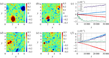
Figure 2 shows snapshots of the barotropic vorticity ( $\unicode[STIX]{x1D701}_{T}$ , a), the baroclinic PV ( $q_{C}$ , b) and the energy spectra (c) of balanced flow ( $E_{B}$ , black) and waves ( $E_{W}$ , red), at $t=30\,000$ for QG (a–c) and CW (d–f) regimes. Initially, the flow in these regimes were seen to develop baroclinic instabilities, leading to turbulence characterized by small-scale structures, which gradually merged and grew, resulting in the formation of large-scale coherent vortices. At the final time corresponding to the state shown in figure 2, most of the energy is contained in the large coherent structures, with negligible small-scale features. The energy changes that accompany this process are shown in figure 3. In both QG and CW cases, the barotropic mode continuously extracts energy from the baroclinic balanced mode, as is expected in two-mode geostrophic turbulent flows (Salmon Reference Salmon1978, Vallis Reference Vallis2006). Nevertheless, the total balanced energy and the total wave energy do not show any noticeable change with time, both being separately conserved.

Figure 2.

Top row shows (a)  $\unicode[STIX]{x1D701}_{T}$ , (b)  $q_{C}$ and (c) energy spectrum for the QG regime at $t=30\,000$ . (d–f) Shows the same quantities for the CW regime. The barotropic, baroclinic balanced and total balanced flow energy spectra – $E_{T}$ , $E_{G}$ and $E_{B}$ – are indistinguishable from each other, which is why only the last one is shown above.

Figure 3.

Energy change versus time (difference in energy from $t=0$ ) for barotropic ( $E_{T}$ , purple); balanced baroclinic ( $E_{G}$ , green); balanced total ( $E_{B}$ , blue); wave ( $E_{W}$ , red); and total ( $E_{total}$ , black) energies versus time for QG (a) and CW (b). Notice that although the barotropic and the baroclinic balanced modes do exchange energy, total balanced energy ( $E_{B}$ ), wave energy ( $E_{W}$ ) and the total energy ( $E_{total}$ ) curves lie on top of each other, showing insignificant changes during the entire simulation.

The phenomenology differs drastically in the SW regime. During the early stages, we observed that the presence of waves inhibited vortex mergers and the formation of coherent vortices, with the balanced fields being dominated by small-scale structures. However, on much longer time scales, vortex mergers were observed to take place, although the continuous interaction between inertia–gravity waves and the vortices keeps generating a wide range of active small-scale filamentary features in the balanced flow field. Such a long time state is shown in figure 4. The PV fields shown in figure 4 may be qualitatively compared with those observed in the forced-dissipative three-dimensional simulations of Barkan et al. (Reference Barkan, Winters and McWilliams2017). Barkan et al., operating at $O(1)$ Rossby numbers to capture submesoscale dynamics, found that waves eroded the coherent vortices (see figures 1 and 3 there). On the other hand, in our SW regime, we observed that inertia–gravity waves affect the coherent vortices in the regime $Ro\ll 1$ , characteristic of mesoscales. Overall we found that the coherent structures are more common and persistent in the barotropic mode compared to the baroclinic balanced flow, the latter consisting of a lot more scattered small-scale features, as may be inferred from figures 4(a) and 4(b).

Figure 4.

(a) The $\unicode[STIX]{x1D701}_{T}$ , (b)  $q_{C}$ and (c) energy spectra for the SW case at $t=30\,000$ . Notice that the domain is rich with a range of small-scale structures, in addition to the large-scale coherent vortices seen in the barotropic field.

Compared to the QG and CW regimes, significant wave–balance energy exchange accompanies the changes we observed in the balanced flow fields in the SW regime, these being quantified in figure 5(a). Observe that the total wave energy (red curve) drops almost linearly with time, while the total balanced energy (blue curve) grows by an equal amount to conserve total energy (black curve). In addition to the total balanced flow gaining energy and waves losing energy, we find that the barotropic balanced mode (purple curve) gains energy while baroclinic balanced mode (green curve) loses energy. To get a better handle on the details of the interaction to uncover the energy transfer pathways, we computed all the nonlinear wave–balance transfer terms resulting in the energy exchange.

Figure 5.

(a) Energy change versus time (difference in energy from $t=0$ ) for barotropic ( $E_{T}$ , purple); balanced baroclinic ( $E_{G}$ , green); balanced total ( $E_{B}$ , blue); wave ( $E_{W}$ , red); and total ( $E_{total}$ , black) energies versus time for the SW regime. Decomposition of energy change of (b) barotropic, (c) baroclinic balanced and (d) waves for the SW case based on equations (3.2).

On applying the wave–balanced flow decomposition given by (2.12) to the governing equations (2.6), we obtain evolution equations for wave and balanced fields. From these equations we form the energy evolution equations for the barotropic flow, baroclinic balanced flow and inertia–gravity waves (for example, the energy equation for the barotropic flow is obtained by multiplying (2.6a ) with the barotropic streamfunction in spectral space). The energy evolution equations for the three components take the form (the reader is referred to Davidson (Reference Davidson2013) for generic derivation of such equations and to Waite (Reference Waite2017) for a specific example)

where $\hat{E}_{T}(k,t)=|\hat{\boldsymbol{v}}_{T}(k,t)|^{2}$ , $\hat{E}_{G}(k,t)=|\hat{\boldsymbol{v}}_{G}(k,t)|^{2}+|\hat{p}_{G}(k,t)|^{2}$ and $\hat{E}_{W}(k,t)=|\hat{\boldsymbol{v}}_{W}(k,t)|^{2}+|\hat{p}_{W}(k,t)|^{2}$ represent barotropic, baroclinic balanced and wave energy at a given wavenumber $k$ . We have grouped terms on the right-hand side based on the specific type of interaction. For example, $\hat{T}_{TTT}(k,t)$ refers to the sum of all nonlinear barotropic triads that project on wavenumber $k$ and $\hat{T}_{TGW}(k,t)$ represents the sum of all barotropic–baroclinic balanced–wave triads that project on $k$ . Similarly other terms follow. The ${\hat{H}}(k,t)$ terms above refer to the hyperdissipation acting at the wavenumber $k$ . On summing equations (3.1) over $k$ from $k=0$ to $k=k_{max}$ , where $k_{max}$ is the largest wavenumber at the chosen resolution, we get the evolution equations for the total energy of the three components. Finally, we integrate the total energy equation of each component from $t=0$ to $t=t$ to get the equations for change in corresponding energies from initial time as Observe that (3.2a ) does not contain $E_{TTT}$ , since the sum of all triadic barotropic interactions must not change the net energy within the barotropic mode demanding that $E_{TTT}=0$ . Additionally, we dropped the energy dissipation terms in the final set of equations given in (3.2), as these were several orders of magnitude lower than the other transfer terms (recall that the total energy is almost conserved in our simulations, as indicated by the black curve in figure 5 a).

In (3.2), $E_{TWW}$ is the sum of all triadic interaction terms involving two wave modes and a barotropic mode and is equal and opposite to $E_{WTW}$ , i.e. $E_{TWW}+E_{WTW}=0$ . A positive $E_{TWW}$ value means that the barotropic mode gains a certain amount of energy from waves, the latter losing the same amount of energy. Similarly, $E_{TGG}$ and $E_{GTG}$ are equal and opposite, i.e. $E_{TGG}+E_{GTG}=0$ , and quantify the amount of energy transferred between the balanced modes alone. A positive value of $E_{TGG}$ implies that the baroclinic balanced flow transfers a certain amount of energy to the barotropic mode, resulting in an equal amount of loss in its own energy, given by $E_{GTG}$ . Finally $E_{TGW}$ , $E_{GTW}$ and $E_{WTG}$ correspond to the sum of mixed wave–barotropic–baroclinic balanced triads with $E_{GTW}+E_{TGW}+E_{WTG}=0$ . A positive value for $E_{GTW}$ and negative values for $E_{TGW}$ and $E_{WTG}$ would mean that the baroclinic balanced flow gains energy from both barotropic mode and waves.

Finally, to quantify the energy budgets, we calculated fractional energy change of the three modes, T, G and W, and the various triads that appear in (3.2). We denote the fractional change associated with each of the variables in (3.2) by adding a $\unicode[STIX]{x1D6E5}$ in front of the variable. For example, the fractional change in the energy of the barotropic mode is $\unicode[STIX]{x0394}E_{T}=(E_{T}(t_{final})-E_{T}(0))/E_{T}(0)$ with $\unicode[STIX]{x0394}E_{TWW}=(E_{TWW}(t_{final})-E_{TWW}(0))/E_{T}(0)$ being part of it due to triadic interactions between waves and the barotropic mode alone. Similarly, $\unicode[STIX]{x0394}E_{G}=(E_{G}(t_{final})-E_{G}(0))/E_{G}(0)$ is the fractional change in the baroclinic balanced flow energy, where $\unicode[STIX]{x0394}E_{GTW}=(E_{GTW}(t_{final})-E_{GTW}(0))/E_{G}(0)$ forms a fraction of it due to triadic interactions involving waves, barotropic mode and the baroclinic balanced flow. Fractional changes due to other triadic interaction terms that are seen in (3.2) were calculated along the same lines, and will be used for the discussion that follow.

To get a handle on the energy changes in the SW regime due to different triadic interactions, we examined the time evolution of the various terms in (3.2), these being shown in figures 5(b), 5(c) and 5(d). We find that waves transfer energy directly to the barotropic mode, as seen from the strictly monotonic increase of the $E_{TWW}$ curve in figure 5(b) and the corresponding decrease in $E_{WTW}$ curve in figure 5(d) for the wave energy budget. The barotropic mode also gains energy due to the direct transfer from the baroclinic balanced mode, as can be seen from the $E_{TGG}$ curve and the corresponding $E_{GTG}$ curve in figures 5(b) and 5(c) respectively. The baroclinic balanced mode does extract some energy from the waves and the barotropic mode. Observe the monotonic increase of the $E_{GTW}$ curve in figure 5(c) with corresponding decreasing curves $E_{TGW}$ and $E_{WTG}$ in figures 5(b) and 5(d). However, this gain in the baroclinic balanced energy is smaller than the energy it transfers directly to the barotropic mode, leading to the net decrease in the baroclinic balanced energy. Overall we find that by the end of our simulation at $t=30\,000$ , the barotropic energy increases, $\unicode[STIX]{x0394}E_{T}=360\,\%$ , with energy gain from waves $\unicode[STIX]{x0394}E_{TWW}=148\,\%$ and from baroclinic balanced flow $\unicode[STIX]{x0394}E_{TGG}=344\,\%$ , which exceeds the energy loss via $\unicode[STIX]{x0394}E_{TGW}=-132\,\%$ . The baroclinic energy decreases, $\unicode[STIX]{x0394}E_{G}=-86\,\%$ , due to its direct transfer to the barotropic flow $\unicode[STIX]{x0394}E_{GTG}=-344\,\%$ exceeding its net gain from waves and barotropic flow $\unicode[STIX]{x0394}E_{GTW}=258\,\%$ . On the other hand, the wave energy, being significantly larger than balanced flow energy, drops only by $\unicode[STIX]{x0394}E_{W}=-1.4\,\%$ during this period. These quantitative energy changes are summarized in the fourth row of table 1, with the second and third rows corresponding to QG and CW regimes discussed before.

Figure 6.

Frequency ( $\unicode[STIX]{x1D714}$ ) spectra for $u_{T}$ (black), $u_{G}$ (blue) and $u_{W}$ (red) for modes with $k=5$ in the (a) QG, (b) CW and (c) SW cases. The spectra shown above were computed by averaging the frequency spectra of 10 wavenumbers $\boldsymbol{k}$ that satisfied $|k-5|<0.01$ . In each case, the spectra were computed using a time series between $t=5000$ and 7000. Observe the peak at $\unicode[STIX]{x1D714}=5.1$ for all three cases, this being the inertia–gravity wave frequency ( $\unicode[STIX]{x1D714}_{W}=\sqrt{1+k^{2}}$ ) at $k=5$ . Panel (d) shows the frequency spectra of slow-balanced fields, obtained after a running time averaging operation is performed based on (3.3). Notice that the slow-balanced fields have negligible high frequency components compared with the total balanced fields shown in (c).

At this point the reader is reminded that our wave–balance decomposition as given in (2.8) and (2.12) is based on the normal modes of the linear equations (2.7). The PV fields, shown in figures 2 and 4 represents our geostrophic balanced field. In the SW regime, wave quantities which are second order in wave amplitude, such as Stokes drift for example, are comparable in strength with the balanced flow. Consequently, nonlinear wave interactions including resonant, near-resonant and non-resonant terms, would directly affect the PV. Disentangling these different wave contributions from the PV field in turbulent flow fields, such as the ones we explore, is highly non-trivial. For the QG, CW and SW regimes discussed so far, we examined the frequency spectra of all low wavenumbers up to $k=12$ and an example corresponding to $k=5$ is given in figure 6. We examined only low wavenumbers since as we shall show below, all the wave–balanced flow energy exchanges in the SW regime take place at wavenumbers $k\leqslant 12$ , i.e. at large scales where waves dominate over balanced flow (recall figure 4 c).

Observe in figure 6 that the linear wave frequency peak (see the red curve) stands out in all three cases – QG (a), CW (b) and SW (c) regimes. Only in the QG case, shown in figure 6(a), the waves have a second dominant contribution at low frequencies, corresponding to the ageostrophic corrections to the balanced flow that does not project on the PV. In the CW and especially in the SW case, waves have a single sharp peak corresponding to the linear wave frequency followed by a rapid decay on either side. The presence of high-frequency oscillations in the spectra of the balanced flow in the SW regime, seen in the black and blue curves in figure 6(c), is the signature of nonlinear wave interactions projecting on the balanced flow. The balanced flow in the SW regime therefore fluctuates on fast wave time scales, although a major part of the balanced energy is associated with the low-frequency ‘slow-balanced component’. To demonstrate this explicitly, especially that the energy change of the balanced flow observed in figure 5(a) corresponds to the energy change associated with the slow-balanced component, we performed a running time average of the balanced flow fields. For example, the time-averaged barotropic $x$ -velocity component was calculated as

We examined the slow-balanced fields for three different time averaging window lengths: $\unicode[STIX]{x1D70F}=10$ , 25 and 50. Figure 6(d) shows the frequency spectra of the slow-balanced fields computed after the time averaging operation was performed with $\unicode[STIX]{x1D70F}=50$ . It is clear that the slow-balanced field has insignificant high-frequency fluctuations. We examined the evolution of the energy of the slow-balanced component as a function of time, against the total balanced energy. This means, for example, we computed the slow-barotropic energy $1/2({\overline{u}_{T}}^{2}+{\overline{v}_{T}}^{2})$ and compared it with the total unaveraged-in-time barotropic energy $1/2({u_{T}}^{2}+{v_{T}}^{2})$ for different time averaging window lengths ( $\unicode[STIX]{x1D70F}$ ). Such a comparison is shown in figure 7 for the case $\unicode[STIX]{x1D70F}=50$ for the duration $t=5000{-}10\,000$ in the SW regime shown in figure 5(a). Observe that the slow-balanced energy curves very well approximate the total balanced energy curves. For all three averaging windows ( $\unicode[STIX]{x1D70F}=10$ , 25 and 50) we observed that the slow-balanced energy was more than 98 % of the total balanced energy. (We present only the case corresponding to $\unicode[STIX]{x1D70F}=50$ in figure 7, since other cases are very similar). This confirms that although the balanced field in the SW regime consists of fast fluctuations, as was clear from the frequency spectra shown in figure 6(c), such fast fluctuations carry a negligible amount of energy and the total balanced flow is dominated by the slow-balanced component. Consequently, we conclude that the energy change associated with the balanced fields shown in figure 5(a) almost entirely coincides with the energy change associated with the slow-balanced fields, as is clear from figure 7.

Table 1.

Summary of numerical experiments discussed in this paper. The first, second and third columns show the experiment, initial balance-to-wave energy ratio and initialization wavenumber. The percentage changes in barotropic, baroclinic and wave energies are shown in the next three columns. Last three columns show the percentage of barotropic energy gain due to direct transfer by waves, percentage of barotropic energy gain due to direct transfer by baroclinic balanced flow and percentage of baroclinic balanced energy gain due to transfer from both waves and the barotropic mode.

In spite of the above discussion, we emphasize that although our wave–balance decomposition, based on the linear equations, robustly captures the linear waves in the SW regime, the balanced flow – this being the dynamical field in geostrophic balance and orthogonal to waves – is influenced by nonlinear wave interactions. The time averaging operation does not filter out the effect of waves on balanced flow, but rather simply allows us to define a slow-balanced flow that evolves on a slow time scale with negligible high-frequency fluctuations (recall figure 6 d). This is because nonlinear wave interaction effects would generate a slow time-averaged contribution to the PV, thus affecting the slow-balanced field. Consequently, it is important to appreciate that nonlinear wave interactions form an integral part of balanced dynamics in the SW regime. In appendix B we compare the linear wave–balanced decomposition with alternate decompositions used for NIW–balanced flow asymptotic models in recent times.

Figure 7.

Slow-balanced energy time series for the barotropic and baroclinic modes, plotted along with total balanced energy during the time interval $t=5000$ –10 000 for the SW case. The purple and green curves correspond to those shown in figure 5(a). Observe that the slow barotropic energy represented by the red curve is smoother than the purple coloured total barotropic energy time series. For a similar comparison of the baroclinic balanced energy, only a few points of the slow energy are shown, by the red dots, since the slow and the total baroclinic balanced energies are indistinguishable from each other. For all three averaging windows ( $\unicode[STIX]{x1D70F}=10$ , 25 and 50), we found that the slow-balanced energy was more than 98 % of the total balanced energy.

With the energy exchange pathways clarified, we ask – at what spatial scales do the above described transfers take place? Recall that wave energy dominates over balanced flow at large scales (see energy spectra in figure 4 c). The cross-over between wave and balanced energies take place approximately at $k=12$ once turbulence is fully developed, and changes only by a small amount after $t=5000$ . Given that the phenomenology observed in SW regime is primarily due to wave energy dominating over balanced flow, it is possible that the energy transfers described via figure 5 take place at large scales. We confirmed this hypothesis by computing all the transfer terms shown in (3.2) by restricting all the fields onto the large scales, i.e. by spectrally truncating all fields by setting $k\geqslant 12$ components to zero, thus retaining only large-scale dynamics, $k<12$ , of all fields. We did this by summing equations (3.1) from $k=0$ to $k=12$ to get the evolution equations at large scales. This was integrated over time to compute the energy change and exchanges at large scales. As seen from figure 8, the energy exchanges that occur at scales $k<12$ capture very well that obtained by summing over all $k$ . This demonstrates that all the energy exchanges seen in the SW regime takes place at large scales, $k<12$ , where the wave energy dominates over balanced energy and with negligible interactions taking place at smaller scales.

Figure 8.

The energy decomposition in the SW case comparing the energy computed using all available wavenumbers (solid lines) with that using wavenumbers truncated to large scales, $k<12$ (dots). Panels (a–d) correspond to the four panels in figure 5, zoomed in over a short time interval from $t=10\,000$ to 11 000. Observe the exceptional agreement between the energy change computed using all wavenumbers and that computed using only large scales, $k<12$ .

Having examined the SW regime with $(E_{B}/E_{W})_{t=0}=Ro^{2}$ in sufficient detail, we examine two other strong wave cases: (i)  $\text{SW}_{a}$ with $(E_{B}/E_{W})_{t=0}=Ro$ (initialized as $(E_{B})_{t=0}=0.4$ and $(E_{W})_{t=0}=4$ ) and (ii)  $\text{SW}_{b}$ with $(E_{B}/E_{W})_{t=0}=Ro^{3}$ (initialized as $(E_{B})_{t=0}=0.004$ and $(E_{W})_{t=0}=4$ ). The balanced energy is respectively higher and lower in these two cases compared to the SW case we discussed before. The spatial structures of the PV fields at $t=30\,000$ and the energy transfers associated with these two cases are shown in figure 9, these being qualitatively similar to the SW case. In figure 9 we find small-scale features in the PV field along with waves transferring energy to the balanced flow. Comparing figures 9(c) and 5(a), we infer that energy transfer between balanced modes exceeds energy exchange between waves and balanced flow in the $\text{SW}_{a}$ case, relative to the SW case (notice that in figure 9(c) the separation between the red and the blue curves is smaller than that between the green and the purple curves). Since the $\text{SW}_{a}$ regime is sandwiched between the CW and SW regimes, we infer that the transition from the CW to SW regime is a gradual one, rather than an abrupt bifurcation, with the $\text{SW}_{a}$ case tending towards the SW case as the ratio $(E_{B}/E_{W})_{t=0}$ is decreased further. We also find that $\text{SW}_{a}$ case comprises of larger and more persistent coherent vortices compared with the SW case presented in figure 4. In contrast, more wave–balance energy exchange and disruption of coherent vortices is observed in the $\text{SW}_{b}$ regime, as can be inferred from figure 9(d–f). Although the energy transfer details in $\text{SW}_{a}$ and $\text{SW}_{b}$ regimes are qualitatively similar to the SW case (figures equivalent to figure 5 b–d are not shown, but energy transfers are quantified in the fifth and sixth rows of table 1), there is an important difference. In the $\text{SW}_{a}$ case, as was the case in the SW regime, the baroclinic balanced flow loses net energy, since the energy it transfers directly to the barotropic mode exceeds its energy gain from the waves and the barotropic mode, i.e. $\unicode[STIX]{x0394}E_{TGG}>\unicode[STIX]{x0394}E_{GTW}$ (notice the drop in the green curve in figure 9 c, similar to that in figure 5 a). In contrast, the baroclinic balanced flow gains more energy from waves and the barotropic mode in the $\text{SW}_{b}$ case, than the amount of energy it transfers directly to the barotropic flow, i.e. $\unicode[STIX]{x0394}E_{TGG}<\unicode[STIX]{x0394}E_{GTW}$ , resulting in an increase in its energy (observe the growth in the green curve in figure 9 f).

Figure 9.

Top row shows the spatial structure of (a)  $\unicode[STIX]{x1D701}_{T}$ and (b)  $q_{C}$ , both at $t=30\,000$ , and (c) energy transfer time series for the $SW_{a}$ case. (d–f) Shows the same quantities for the $SW_{b}$ case.

Our investigation of the energy transfers in the CW, $\text{SW}_{a}$ , SW and $\text{SW}_{b}$ regimes motivate a unified view of these different parameter regimes. Consider a scenario where the flow is initialized with no balanced mode at all, i.e. $(E_{B}/E_{W})=0$ . Waves would feed the balanced flow and increase the $(E_{B}/E_{W})$ ratio. As the flow evolves, the $(E_{B}/E_{W})$ ratio would keep increasing, the flow thereby passing through different regimes we examined: $\text{SW}_{b}$ , SW and $\text{SW}_{a}$ . Eventually, the balanced flow would accumulate enough energy to reach the CW regime, $(E_{B}/E_{W})\sim 1$ , halting the wave–balanced flow energy transfers. However, simulations must proceed to much longer time scales than we have attempted here to demonstrate such gradual transitions between regimes. For example, the change in the energies of wave and the total balanced flow does not seem to diminish in the $\text{SW}_{a}$ regime shown in figure 9(c), even on integrating up to $t=30\,000$ , which corresponds to almost 20 000 eddy turnover time scales. Although we did not observe such inter-regime transitions, even during our relatively long time stimulations, we note the recent detection of such a phenomenon in a small-scale laboratory experiment. Francois et al. (Reference Francois, Xia, Punzmann and Shats2013) observed that externally forced Faraday waves, with wavelengths of the order of a few milimetres, fed two-dimensional turbulence, leading to the formation of large-scale coherent vortices in a laboratory experiment. Of course, although there is a wide range of detailed differences between our problem set at oceanic mesoscales (hundreds of kilometres) and milimetre-scale Faraday waves in the experiment of Francois et al., the qualitative phenomenology is similar: fast waves transferring energy to the slow vortical field and generating large-scale vortices. Consequently, we may think of the laboratory experiment of Francois et al. as a small-scale set-up that achieves the inter-regime transitions we discussed above within a relatively short time scale.

We finally explored the effect of initialization wavenumber in the SW regime. All the simulations discussed so far were initialized with $k_{0}=6$ , a low-mode initialization which gave us a range of wavenumbers for which wave energy dominated over balanced energy in the SW regime (recall figure 4 c where the wave spectrum (red) dominates over balanced spectrum (black) at large scales). Typical oceanic observations indicate a broadband distribution of wavenumbers corresponding to specific tidal frequencies (see for example Ray & Mitchum (Reference Ray and Mitchum1997) and Zhao, Alford & Girton (Reference Zhao, Alford and Girton2012) for observational data on the broad-banded spectral distribution of the $M_{2}$ tidal component). However, there is no generic quantitative estimate for the spectral breadth of the wavenumbers for a fixed-frequency wave field, this of course being sensitive to multiple factors, including the geographic location. Consequently, for completeness, we simulated the SW case with $k_{0}=3$ ( $\text{SW}_{c}$ ) and $k_{0}=12$ ( $\text{SW}_{d}$ ), thereby decreasing and increasing the range of wavenumbers for which wave energy exceeds balanced energy. On doing so we found the same qualitative phenomenology observed so far, with only quantitative changes in the magnitude of energy transfer. For example, in the $\text{SW}_{c}$ regime we found less overall energy transfer compared to the SW case, and vice versa in the $\text{SW}_{d}$ regime. Based on our examination of $\text{SW}_{c}$ and $\text{SW}_{d}$ cases, we infer that the energy transfer from waves to balanced flow is proportional to the range of scales for which wave energy dominates over balanced flow. Additionally, similar to the difference between $\text{SW}_{a}$ and $\text{SW}_{b}$ regimes discussed before, we found that $\unicode[STIX]{x0394}E_{TGG}>\unicode[STIX]{x0394}E_{GTW}$ in the $\text{SW}_{c}$ regime, resulting in the baroclinic balanced flow losing energy with time, while the opposite scenario, $\unicode[STIX]{x0394}E_{TGG}<\unicode[STIX]{x0394}E_{GTW}$ , leading to net increase in baroclinic balanced energy, was seen in the $\text{SW}_{d}$ regime. The energy transfers for these two cases are quantified in the seventh and eighth rows of table 1.

Based on the simulation results presented so far, and several other simulations we performed with slight change in parameter values, we conclude that, except for quantitative changes in the magnitudes of energy transfer, the following phenomenology is robustly observed in all regimes where wave energy dominates over balanced flow energy, i.e. $E_{B}/E_{W}\ll 1$ : The total balanced flow energy increases in all cases ( $\unicode[STIX]{x0394}E_{B}>0$ ), this being due to transfer from waves ( $\unicode[STIX]{x0394}E_{W}<0$ ). The barotropic energy was seen to increase in all regimes, since the energy it extracts directly from waves and baroclinic balanced flow ( $\unicode[STIX]{x0394}E_{TWW}>0$ , $\unicode[STIX]{x0394}E_{TGG}>0$ ) exceeds its energy loss to the baroclinic balanced flow ( $\unicode[STIX]{x0394}E_{TGW}<0$ ). Waves on the other hand were observed to lose energy in all regimes, to the barotropic and baroclinic balanced flow ( $\unicode[STIX]{x0394}E_{WTW}<0$ , $\unicode[STIX]{x0394}E_{WTG}<0$ ). The baroclinic balanced energy was seen to decrease or increase depending on whether it transfers more energy to the barotropic mode than the amount of energy it receives from waves and barotropic mode ( $\unicode[STIX]{x0394}E_{TGG}>\unicode[STIX]{x0394}E_{GTW}$ ) or vice versa. This phenomenology of the net transfers between the two balanced modes and the waves is summarized in the schematic shown in figure 10 and the simulations and the estimates of various energy transfers we reported in this paper so far are given in detail in table 1.

Figure 10.

Energy flow pathways in SW regimes based on our investigation. The blue arrow, as in figure 1, shows direct energy transfer from baroclinic balanced flow to the barotropic balanced flow ( $E_{GTG}$ ), this being the only energy transfer that exists in freely evolving quasi-geostrophic turbulence. In SW regimes, waves transfer energy to the barotropic ( $E_{WTW}$ ) and the baroclinic balanced flow ( $E_{WTG}$ ), as shown by the two red arrows that start on the wave box. The baroclinic balanced flow extracts energy from the barotropic flow ( $E_{TGW}$ ), this being mediated by waves, and is shown by the red arrow that starts on the barotropic box. Overall, the total balanced flow gains energy while waves lose energy. The barotropic mode also gains energy whereas the baroclinic balanced flow may gain or lose energy depending on whether the energy it extracts from waves and the barotropic flow ( $E_{GTW}=E_{WTG}+E_{TGW}$ ) exceeds the energy it loses directly to the barotropic mode ( $E_{GTG}$ ) or vice versa.