1 Introduction
The rotational kinematics and dynamics between two orthonormal triads, or attitude kinematics and dynamics (Hughes Reference Hughes1986) are of essential significance in the study of the relative attitude between two or more rigid bodies, and have broad applications in modern astrophysics, satellite control, aircraft manoeuvre and robotics. Studies on the kinematics and dynamics of rigid-body motions due to mutual interactions (e.g. attraction between celestial bodies) can be traced back to the work of Leonhard Euler (1707–1783), father of analytical dynamics (Battin Reference Battin1999). Further significant developments relevant to the theory of attitude kinematics and dynamics are represented by the classical work Mécanique Analytique by Joseph-Louis Lagrange (1736–1813) and quaternions invented by Sir William R. Hamilton (1805–1865). Founded on these pioneering works, modern research on attitude kinematics and dynamics is still active and keeps advancing in areas such as astrodynamics and spacecraft engineering (Hughes Reference Hughes1986; Shuster Reference Shuster1993; Battin Reference Battin1999), robotic manipulation (Murray, Li & Sastry Reference Murray, Li and Sastry1994), mathematical physics (Angeles Reference Angeles1988) and fluid sciences (Pullin & Saffman Reference Pullin and Saffman1993, Reference Pullin and Saffman1994; Saffman & Pullin Reference Saffman and Pullin1994, Reference Saffman and Pullin1996; Misra & Pullin Reference Misra and Pullin1997; Pullin Reference Pullin2000; Voelkl, Pullin & Chan Reference Voelkl, Pullin and Chan2000; Tao, Katz & Meneveau Reference Tao, Katz and Meneveau2002; Wang, Yee & Bergstrom Reference Wang, Yee and Bergstrom2006b ).
The methodology of attitude kinematics provides an interesting approach for investigating the basic stress–strain relationships encountered in turbulence modelling for the Reynolds-averaged Navier–Stokes (RANS) method and in subgrid-scale (SGS) modelling for large-eddy simulations (LES). Furthermore, some physical processes are determined directly by the relative attitude of the eigenframe triads (or simply, eigenframes) of two tensors. Here, an eigenframe refers to an orthonormal triad formed by the three independent normalized eigenvectors of a second-order real symmetric tensor (such as the SGS stress tensor and resolved strain rate tensor). For example, in the transport process of turbulence kinetic energy (TKE), the TKE production rate is determined by the relative rotation between eigenframes of the Reynolds stress and mean strain rate tensors. Also, the well-known forward and backward scatter phenomena of kinetic energy (KE) between the filtered and subgrid scales in LES are in effect determined by the relative rotation between the eigenframes of the SGS stress and resolved strain rate tensors. The local KE flux is forward scattered if the value of the SGS KE dissipation rate
 ${\it\varepsilon}_{SGS}=-{\it\tau}_{ij}\bar{\unicode[STIX]{x1D61A}}_{ij}$
is positive, and backscatter occurs if the value of
 ${\it\varepsilon}_{SGS}$
is negative (Liu, Meneveau & Katz Reference Liu, Meneveau and Katz1994; Kang & Meneveau Reference Kang and Meneveau2005; Wang & Bergstrom Reference Wang and Bergstrom2005).
According to the classical theory of attitude kinematics and dynamics (Hughes Reference Hughes1986; Angeles Reference Angeles1988; Shuster Reference Shuster1993; Murray et al. Reference Murray, Li and Sastry1994; Battin Reference Battin1999), there are dozens of methods available for describing the relative orientation and rotation of the two orthonormal triads fixed to two rigid bodies. Although these independent methods for attitude representations are all equivalent to each other, care must be taken when a specific method is selected to solve a practical two-rigid-body problem. This is because different choices of methods may affect the efficiency and effectiveness of attitude control (in e.g. satellite orientation positioning and joint motion control in robotics).
Parametrization of the relative orientation and rotation between the eigenframes of two tensors is the first step for the implementation of attitude kinematics into fluid mechanics research. In contrast to the conventional two-rigid-body problem, there is a unique feature in fluid mechanics research: the direction of an eigenvector of a tensor is ambiguous (or aliased) by definition, and a solution needs to be sought in order to eliminate this ambiguity. Thus far, only three types of methods for attitude representation have been reported in the literature of fluid mechanics, i.e. (1) Euler angle triplet, (2) axis–azimuth representation, and (3) Euler rotation angle and axis.
Betchov (Reference Betchov1956) pioneered the application of Euler angle triplet (consisting of three Euler angles) to study the geometrical properties of the velocity gradient tensor (
 $\unicode[STIX]{x1D622}_{ij}\stackrel{\text{def}}{=}\partial _{j}u_{i}$
). This method was later systematically developed by Saffman & Pullin (Reference Saffman and Pullin1994), Pullin & Saffman (Reference Pullin and Saffman1994) and Misra & Pullin (Reference Misra and Pullin1997) for the investigation of eigenframe attitude of the velocity gradient, Reynolds stress and SGS stress tensors. In order to study the eigenframe attitude of the negative of the trace-free SGS stress tensor
 $-{\it\tau}_{ij}^{d}$
with respect to the eigenframe of the resolved strain rate tensor
 $\bar{\unicode[STIX]{x1D61A}}_{ij}\stackrel{\text{def}}{=}(\bar{u}_{i,j}+\bar{u}_{j,i})/2$
, Tao et al. (Reference Tao, Katz and Meneveau2002) and Higgins, Parlange & Meneveau (Reference Higgins, Parlange and Meneveau2003) adopted the axis–azimuth representation, which includes three angles, namely, the colatitude
 ${\it\theta}$
, longitude
 ${\it\phi}$
and azimuthal angle
 ${\it\zeta}$
(see Shuster (Reference Shuster1993) and Tao et al. (Reference Tao, Katz and Meneveau2002) for details of the geometrical description). Here, an overbar indicates a resolved/filtered quantity following the convention of LES.
As reviewed above, to parametrize the attitude of the eigenframe of
 $-{\it\tau}_{ij}^{d}$
with respect to that of
 $\bar{\unicode[STIX]{x1D61A}}_{ij}$
, the conventional method uses either the Euler angle triplet (Pullin & Saffman Reference Pullin and Saffman1994; Saffman & Pullin Reference Saffman and Pullin1994; Misra & Pullin Reference Misra and Pullin1997) or the axis–azimuthal angles (Tao et al.
Reference Tao, Katz and Meneveau2002; Higgins et al.
Reference Higgins, Parlange and Meneveau2003). However, it is noted that the parameters used in both these methods are not uniquely defined. The set of three Euler angles (of the Euler angle triplet) can be parametrized using in total 12 different equivalent ways (six symmetric sets and six asymmetric sets) depending on the method that is adopted for decomposing the relative rotational motion between the two frames, and a similar situation holds for the axis–azimuth representation (Hughes Reference Hughes1986; Shuster Reference Shuster1993).
In view of the non-uniqueness involved in the first two methods, in their technical notes, Wang et al. (Reference Wang, Yee and Bergstrom2006b
) proposed a third method that parametrizes the attitude of the eigenframe of
 $-{\it\tau}_{ij}^{d}$
with respect to that of
 $\bar{\unicode[STIX]{x1D61A}}_{ij}$
based on the classical theorem of Euler. This method uniquely describes the relative attitude between the two eigenframes as a rotation through a special angle
 ${\it\chi}$
(so-called ‘Euler rotation angle’, or simply ‘Euler angle’) about a special fixed axis
 $\boldsymbol{q}$
(so-called ‘Euler axis’). Both Euler angle
 ${\it\chi}$
and Euler axis
 $\boldsymbol{q}$
are ‘natural invariants’ of the rotation matrix (Angeles Reference Angeles1988) between eigenframes of
 $-{\it\tau}_{ij}^{d}$
and
 $\bar{\unicode[STIX]{x1D61A}}_{ij}$
. This proposal constitutes an elegant and unique set of two parameters (one scalar and one vector) for a simple decomposition and invariant representation of the relative rotation between the eigenframes of
 $-{\it\tau}_{ij}^{d}$
and
 $\bar{\unicode[STIX]{x1D61A}}_{ij}$
, and we would regard them as ‘fingerprints’ of an SGS stress model. It should be indicated that the SGS dissipation rate
 ${\it\varepsilon}_{SGS}$
is another important invariant of
 $-{\it\tau}_{ij}^{d}$
and
 $\bar{\unicode[STIX]{x1D61A}}_{ij}$
based on the contraction of these two tensors. Similar to the Euler angle and axis, the value of
 ${\it\varepsilon}_{SGS}$
is unique for an SGS stress model under a specific testing condition and can also be regarded as one of the ‘fingerprints’ of the model. Tensor invariants are important in turbulence study. For instance, the so-called ‘turbulence topology’ focuses on the study of invariants of the Reynolds/SGS stress and strain rate tensors (Perry & Chong Reference Perry and Chong1987; Blackburn, Mansour & Cantwell Reference Blackburn, Mansour and Cantwell1996; van der Bos et al.
Reference van der Bos, Tao, Meneveau and Katz2002; Wang, Bergstrom & Yee Reference Wang, Bergstrom and Yee2006a
), and the so-called ‘Lumley triangle’ focuses on the functional relationship between invariants of the Reynolds stress tensor. The theory of tensor invariants is also important in turbulence and SGS modelling. For instance, Pullin & Saffman (Reference Pullin and Saffman1994), Misra & Pullin (Reference Misra and Pullin1997) and Voelkl et al. (Reference Voelkl, Pullin and Chan2000) built vortex-based SGS models using the eigenframes and eigenvalues of the resolved velocity gradient and strain rate tensors.
Although three attitude representation methods have become available for the study of the tensorial geometric property of the SGS stress tensor over the past two decades, the theory has not been fully set up and even the concept of attitude is relatively new to the LES community. To develop a complete theory that includes all types of parametrizations and representation methods for studying the eigenframe topology of the SGS stress tensor to match similar achievements in established areas such as robotics, spacecraft manoeuvring and satellite control is not yet possible before abundant literature becomes available. The objective of this research focuses on a systematic investigation of the eigenframe topology of the SGS tensor through the representation of the Euler angle and axis. Furthermore, we examine the mathematical procedure for de-aliasing the attitudes of an eigenframe, and aim at proposing an unambiguous method for determining eigenframe topologies of
 $-{\it\tau}_{ij}^{d}$
and
 $\bar{\unicode[STIX]{x1D61A}}_{ij}$
, which finally leads to a standard procedure for calculating the Euler angle and axis of an SGS stress model. In order to prove the effectiveness of the proposed method in studying geometrical properties of SGS stress models, the Euler angle and axis of three different SGS stress models are examined in the context of homogeneous isotropic turbulence at three different Reynolds numbers, using direct numerical simulation (DNS) and both a priori and a posteriori LES approaches.
The remainder of this paper is organized as follows. In § 2, the mathematical representation and improved procedure for calculating the Euler angle and axis are addressed. In § 3, test cases and numerical algorithms for performing DNS and LES are described. In § 4, results on the Euler angle and axis of different SGS stress models based on both a priori and a posteriori approaches are analysed. Finally, in § 5, the major conclusions of this research are summarized.
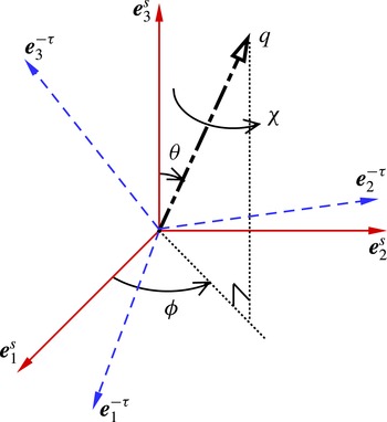
Schematic of the Euler angle and axis due to the relative rotation between the eigenframes (right-handed) of
 $-{\it\tau}_{ij}^{d}$
and
 $\bar{\unicode[STIX]{x1D61A}}_{ij}$
.

2 Topology of the eigenframe of the SGS stress tensor
2.1 Geometrical description of the stress–strain relationship
The relationship between
 $-{\it\tau}_{ij}^{d}$
and
 $\bar{\unicode[STIX]{x1D61A}}_{ij}$
is fundamental for SGS stress modelling, and different types of functional relationships between these two tensors have resulted in many different SGS models ever since the pioneering work of Smagorinsky (Reference Smagorinsky1963) and Lilly (Reference Lilly1966, Reference Lilly1967). In current LES literature, tests of SGS stress models have often focused on their predictive performances in terms of resolved flow structures and statistical moments of different orders (such as the mean velocity, resolved Reynolds shear stresses, resolved TKE and energy spectra). Different from these conventional research focuses, here we further examine the tensorial geometrical properties of the functional relationships between
 $-{\it\tau}_{ij}^{d}$
and
 $\bar{\unicode[STIX]{x1D61A}}_{ij}$
. Because
 $-{\it\tau}_{ij}^{d}$
is a second-order real symmetric tensor, it can be decomposed based on its eigenvalues and eigenvectors as follows:
 $$\begin{eqnarray}\displaystyle -{\it\tau}_{ij}^{d}=\mathop{\sum }_{k=1}^{3}{\it\lambda}_{k}^{-{\it\tau}}e_{k,i}^{-{\it\tau}}e_{k,j}^{-{\it\tau}}. & & \displaystyle\end{eqnarray}$$
Here,
 ${\it\lambda}_{k}^{-{\it\tau}}$
(for
 $k=1$
, 2 and 3) are the three real eigenvalues of
 $-{\it\tau}_{ij}^{d}$
, sorted in a descending order in accordance with their absolute values, i.e.
 $|{\it\lambda}_{1}^{-{\it\tau}}|\geqslant |{\it\lambda}_{2}^{-{\it\tau}}|\geqslant |{\it\lambda}_{3}^{-{\it\tau}}|$
. The eigenvector corresponding to
 ${\it\lambda}_{k}^{-{\it\tau}}$
is denoted by
 $\boldsymbol{e}_{k}^{-{\it\tau}}=[e_{k,1}^{-{\it\tau}},e_{k,2}^{-{\it\tau}},e_{k,3}^{-{\it\tau}}]^{\text{T}}$
, which has been normalized such that its norm is unity identically, i.e.
 $\Vert \boldsymbol{e}_{k}^{-{\it\tau}}\Vert \equiv 1$
. Similar to
 $-{\it\tau}_{ij}^{d}$
, the resolved strain rate tensor
 $\bar{\unicode[STIX]{x1D61A}}_{ij}$
can be decomposed as
 $$\begin{eqnarray}\displaystyle \bar{\unicode[STIX]{x1D61A}}_{ij}=\mathop{\sum }_{k=1}^{3}{\it\lambda}_{k}^{S}e_{k,i}^{S}e_{k,j}^{S}, & & \displaystyle\end{eqnarray}$$
where
 ${\it\lambda}_{k}^{S}$
and
 $\boldsymbol{e}_{k}^{S}=[e_{k,1}^{S},e_{k,2}^{S},e_{k,3}^{S}]^{\text{T}}$
are eigenvalues and normalized eigenvectors of
 $\bar{\unicode[STIX]{x1D61A}}_{ij}$
, respectively. The eigenvalues of
 $\bar{\unicode[STIX]{x1D61A}}_{ij}$
are also arranged in the descending order of their absolute values, i.e.
 $|{\it\lambda}_{1}^{S}|\geqslant |{\it\lambda}_{2}^{S}|\geqslant |{\it\lambda}_{3}^{S}|$
.
From (2.1) and (2.2), it is clear that the mathematical property of a second-order real symmetric tensor,
 $-{\it\tau}_{ij}^{d}$
or
 $\bar{\unicode[STIX]{x1D61A}}_{ij}$
, can be fully recovered from its eigensystem. In their a priori analysis of holographic particle image velocimetry (HPIV) measurement data of a quasi-isotropic flow at the centre of a square duct, Tao et al. (Reference Tao, Katz and Meneveau2002) used a non-dimensional parameter,
 $s^{\ast }=-3\sqrt{6}{\it\lambda}_{1}{\it\lambda}_{2}{\it\lambda}_{3}/({\it\lambda}_{1}^{2}+{\it\lambda}_{2}^{2}+{\it\lambda}_{3}^{2})^{3/2}$
, to study the eigenvalue ratio of
 $-{\it\tau}_{ij}^{d}$
and
 $\bar{\unicode[STIX]{x1D61A}}_{ij}$
. This parametrization method based on
 $s^{\ast }$
was suggested by Lund & Rogers (Reference Lund and Rogers1994), who revised the original proposal of Ashurst et al. (Reference Ashurst, Kerstein, Kerr and Gibson1987) and Kerr (Reference Kerr1987) in order to obtain unbiased statistics in their DNS study of an isotropic turbulent flow. In general, literature on studies of eigenvalues of a single tensor is relatively abundant. In this research, however, we focus our attention on studying the topological relation between the eigenframes of two tensors using the Euler rotation angle and axis. Specifically, the attitude of the eigenframe of
 $-{\it\tau}_{ij}^{d}$
is investigated with respect to that of
 $\bar{\unicode[STIX]{x1D61A}}_{ij}$
.
2.2 Mathematical description of the Euler rotation angle and axis
Figure 1 shows the eigenframes of
 $-{\it\tau}_{ij}^{d}$
and
 $\bar{\unicode[STIX]{x1D61A}}_{ij}$
, both of which are right-handed triads constructed by their three orthonormal eigenvectors, i.e.
 $\boldsymbol{E}^{-{\it\tau}}=[\boldsymbol{e}_{1}^{-{\it\tau}},\boldsymbol{e}_{2}^{-{\it\tau}},\boldsymbol{e}_{3}^{-{\it\tau}}]$
and
 $\boldsymbol{E}^{S}=[\boldsymbol{e}_{1}^{S},\boldsymbol{e}_{2}^{S},\boldsymbol{e}_{3}^{S}]$
, respectively. We use the eigenframe of
 $\bar{\unicode[STIX]{x1D61A}}_{ij}$
as the observer-referenced frame (or the absolute frame), and treat the eigenframe of
 $-{\it\tau}_{ij}^{d}$
as the object-referenced frame (or the relative frame). According to Euler’s theorem, the rotation of the relative eigenframe
 $\boldsymbol{E}^{-{\it\tau}}$
with respect to the absolute eigenframe
 $\boldsymbol{E}^{S}$
is equivalent to the rotation about a fixed axis
 $\boldsymbol{q}$
through an angle
 ${\it\chi}$
. Here, the special angle
 ${\it\chi}$
and axis
 $\boldsymbol{q}$
are the so-called Euler rotation angle and Euler rotation axis, respectively. The rotation of
 $\boldsymbol{E}^{-{\it\tau}}$
with respect to
 $\boldsymbol{E}^{S}$
is shown schematically in figure 1. To quantify the orientation of vector
 $\boldsymbol{q}$
, its colatitude
 ${\it\theta}$
and longitude
 ${\it\phi}$
with respect to eigenframe
 $\boldsymbol{E}^{S}$
are considered.
In order to obtain the mathematical representation of Euler rotation angle and axis, it is important to revisit the properties of rotation matrix
 $\unicode[STIX]{x1D64D}$
between
 $\boldsymbol{E}^{S}$
and
 $\boldsymbol{E}^{-{\it\tau}}$
, because both
 ${\it\chi}$
and
 $\boldsymbol{q}$
are natural invariants of
 $\unicode[STIX]{x1D64D}$
. The rotation matrix
 $\unicode[STIX]{x1D64D}$
relates the two eigenframes
 $\boldsymbol{E}^{S}$
and
 $\boldsymbol{E}^{-{\it\tau}}$
as
 $$\begin{eqnarray}\displaystyle \boldsymbol{E}^{-{\it\tau}}=\unicode[STIX]{x1D64D}\boldsymbol{E}^{S},\quad \boldsymbol{E}^{S}=\unicode[STIX]{x1D64D}^{-1}\boldsymbol{E}^{-{\it\tau}}. & & \displaystyle\end{eqnarray}$$
The Euler angle is determined by the trace of
 $\unicode[STIX]{x1D64D}$
as
 $$\begin{eqnarray}\displaystyle {\it\chi}=\arccos \frac{\text{tr}(\unicode[STIX]{x1D64D})-1}{2}. & & \displaystyle\end{eqnarray}$$
The Euler axis
 $\boldsymbol{q}$
can be calculated from the equation (Hughes Reference Hughes1986; Wang et al.
Reference Wang, Yee and Bergstrom2006b
)
 $$\begin{eqnarray}\displaystyle \unicode[STIX]{x1D666}^{\times }=\frac{\unicode[STIX]{x1D64D}^{\text{T}}-\unicode[STIX]{x1D64D}}{2\sin {\it\chi}}, & & \displaystyle\end{eqnarray}$$
where
 $\unicode[STIX]{x1D666}^{\times }$
represents the following skew-symmetric matrix:
 $$\begin{eqnarray}\displaystyle \unicode[STIX]{x1D666}^{\times }=\left[\begin{array}{@{}ccc@{}}0 & -q_{3} & q_{2}\\ q_{3} & 0 & -q_{1}\\ -q_{2} & q_{1} & 0\end{array}\right]. & & \displaystyle\end{eqnarray}$$
A special characteristic of an eigenvector is that it is ambiguous (or aliased) in direction by definition. If
 $\boldsymbol{e}$
is an eigenvector of tensor
 $\unicode[STIX]{x1D63C}$
, then
 $-\boldsymbol{e}$
must also be an eigenvector of
 $\unicode[STIX]{x1D63C}$
corresponding to the same eigenvalue
 ${\it\lambda}$
. As such, in total, there are four possible right-handed (also four left-handed) eigenframes for both
 $-{\it\tau}_{ij}^{d}$
and
 $\bar{\unicode[STIX]{x1D61A}}_{ij}$
. Let
 $[\boldsymbol{e}_{1}^{S},\boldsymbol{e}_{2}^{S},\boldsymbol{e}_{3}^{S}]$
represent a right-handed eigenframe of
 $\bar{\unicode[STIX]{x1D61A}}_{ij}$
; the following gives the complete set of four scenarios of right-handed eigenframes of
 $\bar{\unicode[STIX]{x1D61A}}_{ij}$
:
 $$\begin{eqnarray}\displaystyle \left.\begin{array}{@{}c@{}}\boldsymbol{E}_{0}^{S}\stackrel{\text{def}}{=}[\boldsymbol{e}_{1}^{S},\boldsymbol{e}_{2}^{S},\boldsymbol{e}_{3}^{S}],\\ \boldsymbol{E}_{1}^{S}\stackrel{\text{def}}{=}[\boldsymbol{e}_{1}^{S},-\boldsymbol{e}_{2}^{S},-\boldsymbol{e}_{3}^{S}],\\ \boldsymbol{E}_{2}^{S}\stackrel{\text{def}}{=}[-\boldsymbol{e}_{1}^{S},\boldsymbol{e}_{2}^{S},-\boldsymbol{e}_{3}^{S}],\\ \boldsymbol{E}_{3}^{S}\stackrel{\text{def}}{=}[-\boldsymbol{e}_{1}^{S},-\boldsymbol{e}_{2}^{S},\boldsymbol{e}_{3}^{S}].\end{array}\right\} & & \displaystyle\end{eqnarray}$$
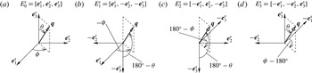
Figure 2 shows the topologies of a fixed Euler axis
 $\boldsymbol{q}$
with respect to the above four right-handed eigenframes of
 $\bar{\unicode[STIX]{x1D61A}}_{ij}$
. Similarly, the SGS stress tensor
 $-{\it\tau}_{ij}^{d}$
also has four possible right-handed eigenframes:
 $$\begin{eqnarray}\displaystyle \left.\begin{array}{@{}c@{}}\boldsymbol{E}_{0}^{-{\it\tau}}\stackrel{\text{def}}{=}[\boldsymbol{e}_{1}^{-{\it\tau}},\boldsymbol{e}_{2}^{-{\it\tau}},\boldsymbol{e}_{3}^{-{\it\tau}}],\\ \boldsymbol{E}_{1}^{-{\it\tau}}\stackrel{\text{def}}{=}[\boldsymbol{e}_{1}^{-{\it\tau}},-\boldsymbol{e}_{2}^{-{\it\tau}},-\boldsymbol{e}_{3}^{-{\it\tau}}],\\ \boldsymbol{E}_{2}^{-{\it\tau}}\stackrel{\text{def}}{=}[-\boldsymbol{e}_{1}^{-{\it\tau}},\boldsymbol{e}_{2}^{-{\it\tau}},-\boldsymbol{e}_{3}^{-{\it\tau}}],\\ \boldsymbol{E}_{3}^{-{\it\tau}}\stackrel{\text{def}}{=}[-\boldsymbol{e}_{1}^{-{\it\tau}},-\boldsymbol{e}_{2}^{-{\it\tau}},\boldsymbol{e}_{3}^{-{\it\tau}}].\end{array}\right\} & & \displaystyle\end{eqnarray}$$
Considering the fundamental difference between an eigenframe of a tensor and a triad fixed to a rigid body, in order to apply Euler’s theorem to the investigation of relative attitude between the eigen-ellipsoids of two tensors, an additional procedure is needed to eliminate any ambiguity involved in the topology of eigenframes. To make the procedure general, firstly, we arbitrarily select an eigenframe of
 $\bar{\unicode[STIX]{x1D61A}}_{ij}$
and denote it as
 $\boldsymbol{E}_{0}^{S}$
. Then, the other three eigenframes
 $\boldsymbol{E}_{1}^{S}$
,
 $\boldsymbol{E}_{2}^{S}$
and
 $\boldsymbol{E}_{3}^{S}$
in (2.7) are determined subsequently. By default, we define
 $\boldsymbol{E}_{0}^{S}$
as the absolute frame, i.e.
 $\boldsymbol{E}^{S}\stackrel{\text{def}}{=}\boldsymbol{E}_{0}^{S}$
. Secondly, in order to select the relative frame
 $\boldsymbol{E}^{-{\it\tau}}$
from the four scenarios given in (2.8), we introduce a criterion that requires the value of the Euler angle
 ${\it\chi}$
to be minimum. Without losing generality in mathematical notation, let this special relative eigenframe be represented by
 $\boldsymbol{E}_{0}^{-{\it\tau}}$
, and define it as
 $\boldsymbol{E}^{-{\it\tau}}$
(i.e.
 $\boldsymbol{E}^{-{\it\tau}}\stackrel{\text{def}}{=}\boldsymbol{E}_{0}^{-{\it\tau}}$
). Subsequently, the other three eigenframes
 $\boldsymbol{E}_{1}^{-{\it\tau}}$
,
 $\boldsymbol{E}_{2}^{-{\it\tau}}$
and
 $\boldsymbol{E}_{3}^{-{\it\tau}}$
in (2.8) are determined. From (2.3), we obtain
 $\boldsymbol{E}_{0}^{-{\it\tau}}=\unicode[STIX]{x1D64D}\boldsymbol{E}_{0}^{S}$
. It is then straightforward to show from (2.7) and (2.8) that
 $\unicode[STIX]{x1D64D}$
is also the rotation matrix between
 $\boldsymbol{E}_{i}^{-{\it\tau}}$
and
 $\boldsymbol{E}_{i}^{S}$
for the other three scenarios. All together, we have
 $$\begin{eqnarray}\displaystyle \boldsymbol{E}_{i}^{-{\it\tau}}=\unicode[STIX]{x1D64D}\boldsymbol{E}_{i}^{S}\quad (\text{for }i=0,1,2\text{ and }3). & & \displaystyle\end{eqnarray}$$
As natural invariants of the rotation matrix
 $\unicode[STIX]{x1D64D}$
, the Euler angle
 ${\it\chi}$
and Euler axis
 $\boldsymbol{q}$
should be independent of the initial arbitrary choice of
 $\boldsymbol{E}_{0}^{S}$
. However, the relative orientation of
 $\boldsymbol{q}$
is determined by the selected eigenframe
 $\boldsymbol{E}_{0}^{S}$
, which is evident from figure 2. As shown in figure 2, this topology indicated by
 $({\it\theta},{\it\phi})$
is aliased with the other three possibilities, i.e.
 $(180^{\circ }-{\it\theta},-{\it\phi})$
,
 $(180^{\circ }-{\it\theta},180^{\circ }-{\it\phi})$
and
 $({\it\theta},{\it\phi}-180^{\circ })$
with respect to eigenframes
 $\boldsymbol{E}_{1}^{S}$
,
 $\boldsymbol{E}_{2}^{S}$
and
 $\boldsymbol{E}_{3}^{S}$
, respectively. As a direct consequence of aliasing, if
 $\boldsymbol{E}^{S}$
is randomly selected from
 $\boldsymbol{E}_{i}^{S}$
(for
 $i=0$
, 1, 2 and 3), the joint probability density function (JPDF) of
 $({\it\theta},{\it\phi})$
of each of these four scenarios are expected to be identical, i.e.
 $$\begin{eqnarray}\displaystyle P({\it\theta},{\it\phi})=P(180^{\circ }-{\it\theta},-{\it\phi})=P(180^{\circ }-{\it\theta},180^{\circ }-{\it\phi})=P({\it\theta},{\it\phi}-180^{\circ }). & & \displaystyle\end{eqnarray}$$
To calculate the JPDF
 $P({\it\theta},{\it\phi})$
, the ranges of
 ${\it\theta}$
and
 ${\it\phi}$
are divided uniformly into
 $50\times 50$
bins; thus the area of each bin is
 ${\it\Sigma}={\rm\Delta}{\it\theta}{\rm\Delta}{\it\phi}$
identically. However, the uniform bins in the
 $({\it\theta},{\it\phi})$
plane are distorted by the spherical curvature, and as such the bin area over the surface of a unit sphere is
 $S_{{\it\Sigma}}=\sin {\it\theta}\,{\rm\Delta}{\it\theta}{\rm\Delta}{\it\phi}$
. Here,
 $S_{{\it\Sigma}}$
is the so-called solid angle, which varies with
 ${\it\theta}$
. In order to present an unbiased view of the JPDF values obtained over the surface of a three-dimensional (3D) unit sphere in a two-dimensional (2D)
 $({\it\theta},{\it\phi})$
plane, the effect of spherical curvature needs to be considered. To this purpose, the following pre-multiplied JPDF is used:
 $$\begin{eqnarray}\displaystyle P_{m}({\it\theta},{\it\phi})\stackrel{\text{def}}{=}P({\it\theta},{\it\phi})\sin {\it\theta}. & & \displaystyle\end{eqnarray}$$
In their study of the alignment between eigenvectors of the SGS stress and resolved strain rate tensor, Tao et al. (Reference Tao, Katz and Meneveau2002) and Higgins et al. (Reference Higgins, Parlange and Meneveau2003) considered the JPDF of
 $(\cos {\it\theta},{\it\phi})$
, which method is equivalent to the current approach based on the solid angle, simply because
 $S_{{\it\Sigma}}=\sin {\it\theta}\,{\rm\Delta}{\it\theta}{\rm\Delta}{\it\phi}\approx {\rm\Delta}(\cos {\it\theta}){\rm\Delta}{\it\phi}$
. The pre-multiplied JPDF
 $P_{m}({\it\theta},{\it\phi})$
defined in (2.11) should obey the following identity in a 2D
 $({\it\theta},{\it\phi})$
plane:
 $$\begin{eqnarray}\displaystyle P_{m}({\it\theta},{\it\phi})=P_{m}(180^{\circ }-{\it\theta},-{\it\phi})=P_{m}(180^{\circ }-{\it\theta},180^{\circ }-{\it\phi})=P_{m}({\it\theta},{\it\phi}-180^{\circ }), & & \displaystyle\end{eqnarray}$$
which is equivalent to that given by (2.10) based on the surface of a 3D unit sphere.
Orientation of the Euler axis described using colatitude and longitude with respect to four scenarios of right-handed eigenframes of
 $\bar{\unicode[STIX]{x1D61A}}_{ij}$
.

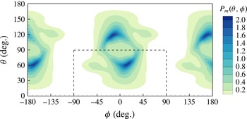
Contours of pre-multiplied JPDF
 $P_{m}({\it\theta},{\it\phi})$
at
 $Re_{{\it\tau}}=272$
obtained from DNS displayed in the 2D
 $({\it\theta},{\it\phi})$
plane. The eigenframe
 $\boldsymbol{E}^{S}$
is arbitrarily selected from
 $\boldsymbol{E}_{i}^{S}$
for
 $i=0$
, 1, 2 and 3. Contours corresponding to lower probability densities (
 $P_{m}({\it\theta},{\it\phi})<0.5$
) are clipped.

To verify the above identity, we can examine the DNS results of
 $P_{m}({\it\theta},{\it\phi})$
. The numerical algorithm for generating the DNS data and the filtering process used for extracting
 ${\it\tau}_{ij}$
are to be introduced later in § 3. Figure 3 shows the DNS result of
 $P_{m}({\it\theta},{\it\phi})$
with the eigenframe of
 $\bar{\unicode[STIX]{x1D61A}}_{ij}$
being randomly selected from
 $\boldsymbol{E}_{i}^{S}$
(for
 $i=0$
, 1, 2 and 3). From figure 3, altogether four dominant modes of
 $P_{m}({\it\theta},{\it\phi})$
are observed, which are located at
 $({\it\theta},{\it\phi})=(62^{\circ },15^{\circ })$
,
 $(118^{\circ },-15^{\circ })$
,
 $(118^{\circ },165^{\circ })$
and
 $(62^{\circ },-165^{\circ })$
. Clearly, the distribution of these four modes strictly obeys the identity dictated by (2.12). Furthermore, (2.12) requires that the distribution of these four modes be symmetrical about the centre of the domain,
 $({\it\theta},{\it\phi})=(90^{\circ },0^{\circ })$
. From figure 3, it is evident that this central symmetry property of
 $P_{m}({\it\theta},{\it\phi})$
has been verified numerically by DNS. Owing to this central symmetry property, it is guaranteed that one and only one of the four modes falls within an arbitrary quarter (constituted by one half the range for each of the two variables
 ${\it\theta}$
and
 ${\it\phi}$
) of the domain
 $([0^{\circ },180^{\circ }],[-180^{\circ },180^{\circ }])$
. This allows us to eliminate the ambiguity during the procedure of selecting the absolute eigenframe
 $\boldsymbol{E}^{S}$
out of the four possibilities. We define the eigenframe of
 $\bar{\unicode[STIX]{x1D61A}}_{ij}$
as the absolute frame if and only if the state corresponding to the combined values of
 $({\it\theta},{\it\phi})$
falls within the following quarter of the domain,
 $([0^{\circ },90^{\circ }],[-90^{\circ },90^{\circ }])$
. This selected quarter of the domain is highlighted using a dashed box in figure 3. It should be indicated that, although the choice of this specific quarter of the domain for defining the absolute frame is arbitrary, it does not alter our understanding of the relative attitude between the eigenframes of
 $-{\it\tau}_{ij}^{d}$
and
 $\bar{\unicode[STIX]{x1D61A}}_{ij}$
in terms of the theory and uniqueness of the statistical results.
In conclusion, in order to study the eigenframe attitude of
 $-{\it\tau}_{ij}^{d}$
with respect to that of
 $\bar{\unicode[STIX]{x1D61A}}_{ij}$
, the aliasing of the eigenframe topology intrinsic to these two tensors needs to be removed. The procedure for calculating the Euler angle and axis between the eigenframes of
 $-{\it\tau}_{ij}^{d}$
and
 $\bar{\unicode[STIX]{x1D61A}}_{ij}$
can be summarized as follows:
Step 1. Calculate the eigensystems of these two tensors and sort the eigenvalues in the descending order of their absolute values. Define the eigenframe as a right-handed triad constructed by the three orthonormal eigenvectors of a tensor.
Step 2. Choose an eigenframe of
 $\bar{\unicode[STIX]{x1D61A}}_{ij}$
arbitrarily, and select the eigenframe of
 $-{\it\tau}_{ij}^{d}$
that makes the Euler angle minimal.
Step 3. Calculate the rotation matrix
 $\unicode[STIX]{x1D64D}$
, Euler angle
 ${\it\chi}$
and Euler axis
 $\boldsymbol{q}$
.
Step 4. Select the eigenframe of
 $\bar{\unicode[STIX]{x1D61A}}_{ij}$
as the absolute frame if
 $({\it\theta},{\it\phi})\in ([0^{\circ },90^{\circ }],[-90^{\circ },90^{\circ }])$
.
3 Numerical methods and test cases
3.1 Governing equations
In order to study the eigenframe topology of the SGS stress tensor in the context of homogeneous isotropic turbulence using both a priori and a posteriori LES approaches, both DNS and LES need to be performed. The continuity and momentum equations that govern the turbulent flow fields for both DNS and LES can be written in the following general form in the context of an incompressible fluid:
 $$\begin{eqnarray}\displaystyle & \displaystyle \frac{\partial \bar{u}_{i}}{\partial x_{i}}=0, & \displaystyle\end{eqnarray}$$
 $$\begin{eqnarray}\displaystyle & \displaystyle \frac{\partial \bar{u}_{i}}{\partial t}+\bar{u}_{j}\frac{\partial \bar{u}_{i}}{\partial x_{j}}=-\frac{1}{{\it\rho}}\frac{\partial \bar{p}}{\partial x_{i}}+{\it\nu}\frac{\partial ^{2}\bar{u}_{i}}{\partial x_{j}\partial x_{j}}-\frac{\partial {\it\tau}_{ij}^{d}}{\partial x_{j}}+f_{i}. & \displaystyle\end{eqnarray}$$
 $f_{i}$
represents an artificial forcing, which injects energy into turbulence to balance the dissipation in order to sustain the TKE level. The specific formulation of
 $f_{i}$
will be given later in § 3.2 along with the introduction of the algorithm for generating homogeneous turbulence. In (3.1) and (3.2), the overbar represents a grid level filtering operation in LES. However, in DNS, no filtering process is involved and the grid size should be comparable to the Kolmogorov scale. For DNS, term
 ${\it\tau}_{ij}^{d}$
is simply set to zero; however, for LES, it represents the SGS stress tensor, defined as
 ${\it\tau}_{ij}=\overline{u_{i}u}_{j}-\bar{u}_{i}\bar{u}_{j}$
. Here, superscript
 $d$
is used to denote the deviatoric part of a tensor, i.e.
 $(\cdot )^{d}=(\cdot )_{ij}-(\cdot )_{kk}{\it\delta}_{ij}/3$
, with
 ${\it\delta}_{ij}$
being the Kronecker delta. In a conventional LES approach, only the deviatoric part of the SGS stress tensor
 ${\it\tau}_{ij}^{d}$
is modelled, and the trace of
 ${\it\tau}_{ij}$
is absorbed into the effective pressure term. The proposed parametrization method for the Euler angle and axis will be utilized to study the eigenframe topology of three different SGS stress models, which include (1) the dynamic Smagorinsky model (DSM) of Lilly (Reference Lilly1992), (2) the dynamic two-parameter mixed model (DMM) of Morinishi & Vasilyev (Reference Morinishi and Vasilyev2001), and (3) the dynamic nonlinear model (DNM) of Wang & Bergstrom (Reference Wang and Bergstrom2005).
In order to make the paper concise and make it convenient for computer coding, these three SGS stress models can be elegantly expressed using the general equation
 $$\begin{eqnarray}\displaystyle {\it\tau}_{ij}^{d}=-C_{M}D\bar{\unicode[STIX]{x1D61A}}_{ij}-C_{W}E{\it\gamma}_{ij}-C_{N}E{\it\eta}_{ij}, & & \displaystyle\end{eqnarray}$$
where
 $C_{M}$
,
 $C_{W}$
and
 $C_{N}$
are model coefficients that can be determined dynamically. In the above equation, the first term is linear because it follows the Boussinesq hypothesis (i.e.
 $-{\it\tau}_{ij}^{d}\propto \bar{\unicode[STIX]{x1D61A}}_{ij}$
), whereas the second and third terms are nonlinear, as they do not follow this hypothesis. Different functional expressions of
 $D$
,
 $E$
,
 ${\it\gamma}_{ij}$
and
 ${\it\eta}_{ij}$
result in different SGS stress models. For the DSM,
 $$\begin{eqnarray}\displaystyle D=2\bar{{\it\Delta}}^{2}|\bar{S}|,\quad E\equiv 0,\quad {\it\gamma}_{ij}\equiv 0,\quad {\it\eta}_{ij}\equiv 0. & & \displaystyle\end{eqnarray}$$
For the DMM,
 $$\begin{eqnarray}\displaystyle D=2\bar{{\it\Delta}}^{2}|\bar{S}|,\quad E\equiv -1,\quad {\it\gamma}_{ij}=(\overline{\bar{u}_{i}\bar{u}}_{j}-\bar{\bar{u}}_{i}\bar{\bar{u}}_{j})^{d},\quad {\it\eta}_{ij}\equiv 0. & & \displaystyle\end{eqnarray}$$
For the DNM,
 $$\begin{eqnarray}\displaystyle D=2\bar{{\it\Delta}}^{2}|\bar{S}|,\quad E=4\bar{{\it\Delta}}^{2},\quad {\it\gamma}_{ij}=\bar{S}_{ik}\bar{{\it\Omega}}_{kj}+\bar{S}_{jk}\bar{{\it\Omega}}_{ki},\quad {\it\eta}_{ij}=(\bar{S}_{ik}\bar{S}_{kj})^{d}. & & \displaystyle\end{eqnarray}$$
Here,
 $|\bar{S}|=(2\bar{\unicode[STIX]{x1D61A}}_{ij}\bar{\unicode[STIX]{x1D61A}}_{ij})^{1/2}$
is the norm of
 $\bar{\unicode[STIX]{x1D61A}}_{ij}$
,
 $\bar{{\it\Delta}}$
is the grid level filter size, and
 $\bar{{\it\Omega}}_{ij}=(\partial \bar{u}_{i}/\partial x_{j}-\partial \bar{u}_{j}/\partial x_{i})/2$
is the resolved rotation rate tensor.
3.2 Algorithms for DNS and LES
In order to conduct both a priori and a posteriori studies, DNS and LES data are generated using an in-house pseudo-spectral method code. The algorithm of the code follows Eswaran & Pope (Reference Eswaran and Pope1988). The number of grid points is set to
 $N^{3}$
and periodic conditions are imposed in all three directions of a cubic domain. A variable
 ${\it\phi}(\boldsymbol{x},t)$
in the physical space is expanded into discrete Fourier series
 $\hat{{\it\phi}}(\boldsymbol{k},t)$
, where
 $\boldsymbol{k}=[k_{1},k_{2},k_{3}]^{\text{T}}=[m_{1}k_{0},m_{2}k_{0},m_{3}k_{0}]^{\text{T}}$
is the wavenumber vector, with
 $k_{0}$
being the lowest positive wavenumber, and
 $m_{1}$
,
 $m_{2}$
and
 $m_{3}$
all being integers between
 $-N/2$
and
 $N/2-1$
. The convection term in (3.2) needs to be calculated in the physical space and the aliasing error is removed using the
 $3/2$
rule. The time advancement is achieved by using a fourth-order explicit Runge–Kutta scheme.
In order to sustain the TKE at a statistically stationary level, the artificial body force
 $f_{i}$
proposed by Carati, Ghosal & Moin (Reference Carati, Ghosal and Moin1995) is included in (3.2), which reads
 $$\begin{eqnarray}\displaystyle \hat{\boldsymbol{f}}(\boldsymbol{k},t)=\frac{{\it\epsilon}_{f}}{N_{f}}\frac{\hat{\bar{\boldsymbol{u}}}(\boldsymbol{k},t)}{\hat{\bar{\boldsymbol{u}}}(\boldsymbol{k},t)\boldsymbol{\cdot }\hat{\bar{\boldsymbol{u}}}^{\ast }(\boldsymbol{k},t)}\quad (\text{for }k_{0}\leqslant k\leqslant k_{f}), & & \displaystyle\end{eqnarray}$$
where an asterisk represents the conjugate of a complex number,
 $\hat{\bar{\boldsymbol{u}}}$
is the Fourier transform of the resolved velocity,
 $N_{f}$
represents the number of modes inside the shell determined automatically by the shell radius
 $k_{f}$
, and
 $k=\Vert \boldsymbol{k}\Vert$
is the vector norm of
 $\boldsymbol{k}$
. The forcing is applied inside the shell for
 $k_{0}\leqslant k\leqslant k_{f}$
. Following Eswaran & Pope (Reference Eswaran and Pope1988), the value of
 $k_{f}/k_{0}$
is set to
 $\sqrt{2}$
, and in consequence
 $N_{f}=18$
. The forcing intensity is controlled by the energy injection rate
 ${\it\epsilon}_{f}$
, which is set to a constant value 0.15 to balance the overall dissipation rate.
3.3 Test cases and grid resolutions
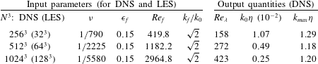
Three DNS databases were generated in order to perform the a priori study. Table 1 summarizes input parameters for controlling DNS and LES and important output quantities of DNS. As shown in table 1, three DNS test cases were carried out with grid points of
 $N^{3}=256^{3}$
,
 $512^{3}$
and
 $1024^{3}$
. As indicated by Eswaran & Pope (Reference Eswaran and Pope1988), the flow is controlled by three non-dimensional parameters:
 $N$
,
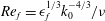 $Re_{f}={\it\epsilon}_{f}^{1/3}k_{0}^{-4/3}/{\it\nu}$
and
 $k_{f}/k_{0}$
. Here,
 $Re_{f}$
is the so-called forcing Reynolds number, whose value is
 $419.8$
,
 $1182.2$
and
 $2964.8$
for the three test cases considered. As an output parameter of DNS, the Taylor-microscale Reynolds number (or Reynolds number hereafter for simplicity) is an important characteristic of homogeneous isotropic turbulence. It is defined as
 $Re_{{\it\lambda}}=u^{\prime }{\it\lambda}/{\it\nu}$
, where
 ${\it\lambda}=(15{\it\nu}u^{\prime 2}/{\it\epsilon})^{0.5}$
represents the Taylor microscale and the fluctuating velocity scale
 $u^{\prime }$
is determined from the TKE
 $k_{u}$
as
 $u^{\prime 2}=2k_{u}/3$
. The Reynolds number calculated by DNS for the three cases is
 $Re_{{\it\lambda}}=158$
, 272 and 423, respectively. It is evident from table 1 that the strict criterion suggested by Eswaran & Pope (Reference Eswaran and Pope1988) on grid resolution for ‘good’ DNS (i.e.
 $k_{max}{\it\eta}>1$
) is well satisfied in all three DNS test cases. Here,
 $k_{max}=\sqrt{2}Nk_{0}/3$
is the maximum wavenumber resolved and
 ${\it\eta}=({\it\nu}^{3}/{\it\epsilon})^{1/4}$
is the Kolmogorov length scale.
Key input parameters for DNS and LES, and output quantities from DNS of homogeneous isotropic turbulence.
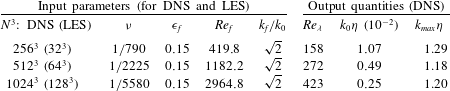
In order to further investigate the Euler angle and axis of SGS stress models using the a posteriori approach, LES of homogeneous isotropic turbulence is also conducted. Similar to a priori tests, three test cases of the same Reynolds numbers are considered in our a posteriori study. The number of grid points is
 $N^{3}=32^{3}$
,
 $64^{3}$
and
 $128^{3}$
for
 $Re_{{\it\lambda}}=158$
, 272 and 423, respectively. Other input parameters for LES (e.g.
 $Re_{f}$
and
 $k_{f}/k_{0}$
) are identical to those for DNS, which are summarized in table 1.
3.4 Discrete filters
A discrete filter is needed in both a priori and a posteriori tests. To this purpose, there are many different types of discrete filters available in the literature. The current procedure for performing a priori tests follows the method of Tao et al. (Reference Tao, Katz and Meneveau2002), who used discrete box filters to process wind tunnel measurement data in their a priori LES study of SGS stress models. The resolved velocity field
 $\bar{u}_{i}$
is extracted from the DNS data using the following fourth-order discrete box filter proposed by Sagaut & Grohens (Reference Sagaut and Grohens1999):
 $$\begin{eqnarray}\displaystyle \bar{{\it\phi}}(x_{1},x_{2},x_{3}) & = & \displaystyle \frac{1}{3}\mathop{\sum }_{i=-2}^{2}a_{i} [{\it\phi}(x_{1}+\text{i}{\it\Delta}_{s},x_{2},x_{3})+{\it\phi}(x_{1},x_{2}+\text{i}{\it\Delta}_{s},x_{3})\nonumber\\ \displaystyle & & \displaystyle +\,{\it\phi}(x_{1},x_{2},x_{3}+\text{i}{\it\Delta}_{s})]+O({\it\Delta}_{s}^{4}),\end{eqnarray}$$
where
 ${\it\Delta}_{s}$
represents the stencil separation (i.e. the distance between two adjacent stencil points used for performing the filtering operation). The values of coefficients
 $a_{i}$
are given as
 $$\begin{eqnarray}\displaystyle a_{0}=\frac{3{\it\zeta}^{4}-100{\it\zeta}^{2}+960}{960},\quad a_{-1}=a_{1}=\frac{-3{\it\zeta}^{4}+80{\it\zeta}^{2}}{1440},\quad a_{-2}=a_{2}=\frac{3{\it\zeta}^{4}-20{\it\zeta}^{2}}{5760}, & & \displaystyle \nonumber\\ \displaystyle & & \displaystyle\end{eqnarray}$$
where
 ${\it\zeta}=\bar{{\it\Delta}}/{\it\Delta}_{s}$
represents the ratio of the filter size
 $\bar{{\it\Delta}}$
to the stencil separation
 ${\it\Delta}_{s}$
. In order to conduct the grid level filtering process, the stencil separation and filter size are set to four and eight times the grid size (
 ${\it\Delta}$
) of DNS, respectively, i.e.
 ${\it\Delta}_{s}=4{\it\Delta}$
and
 $\bar{{\it\Delta}}=8{\it\Delta}$
, and, as such, the ratio
 ${\it\zeta}$
is equal to 2. A test-grid level filter is needed to calculate the model coefficients for all three dynamic models described in § 3. The same fourth-order box filter given by (3.8) and (3.9) is used to perform the test-grid level filtering process. However,
 $\bar{{\it\phi}}$
in (3.8) needs to be replaced with
 $\tilde{\bar{{\it\phi}}}$
, and ratio
 ${\it\zeta}$
in (3.9) should be redefined as
 $\tilde{\bar{{\it\Delta}}}/\bar{{\it\Delta}}$
. Following the usual convention, the filter size at the test-grid level is kept twice that at the grid level, i.e.
 $\tilde{\bar{{\it\Delta}}}=2\bar{{\it\Delta}}$
. In order to perform genuine LES using dynamic SGS stress models, it is important to ensure that the cutoff filter sizes at both grid and test-grid levels fall within the inertial subrange. The examination of the inertial subrange based on the energy spectra of homogeneous isotropic turbulence at three different Reynolds numbers will be presented later in § 4.1.
In contrast to the a priori approach described above, in the a posteriori approach, LES needs to be performed with a modelled SGS stress tensor. Following the convention, the resolved velocity field
 $\bar{u}_{i}$
in an a posteriori test is implicitly filtered at the grid level by default, with its filter size equal to the grid size, i.e.
 $\bar{{\it\Delta}}={\it\Delta}$
. The filtering processes involved in the current a posteriori tests are associated with the dynamic modelling procedure. Similar to the a priori approach described above, the filter size ratio between the test-grid and grid levels is also set to
 ${\it\zeta}=\tilde{\bar{{\it\Delta}}}/\bar{{\it\Delta}}=2$
in the a posteriori approach.
4 Result analysis
As an important benchmark test case for studying turbulence phenomena, homogeneous isotropic turbulence provides an idealized turbulent environment that is free from any mean pressure gradients and mean viscous shear stresses. A unique feature of homogeneous isotropic turbulence is that all statistics are independent of the spatial location, which are instead functions of the Reynolds number
 $Re_{{\it\lambda}}$
only. For this benchmark test case, we have two research objectives: (1) in order to determine the Reynolds-number effects on the eigenframe topology of the exact or a modelled SGS stress tensor, a comparative study based on three Reynolds numbers is performed using both DNS and LES; and furthermore, (2) in order to study the modelling effects on the eigenframe topology of the SGS stress tensor, three different SGS stress models are compared using both a priori and a posteriori LES approaches.
4.1 DNS results
The DNS data are used towards the following two purposes:
-
(1) Firstly, as introduced in § 3.4, the values of
 ${\it\tau}_{ij}$
and
$\bar{\unicode[STIX]{x1D61A}}_{ij}$
can be directly extracted by filtering DNS data strictly based on their definitions (without involving any specific SGS stress models). The obtained results on the Euler angle and axis will be referred to as ‘DNS results’, which facilitate a precise analysis of the eigenframe topology of the SGS stress tensor and can be further used for validating both a priori and a posteriori LES results (both involving SGS stress model effects).
-
(2) Secondly, the DNS databases are fundamental for the follow-up a priori LES analysis of the Euler angle and axis.


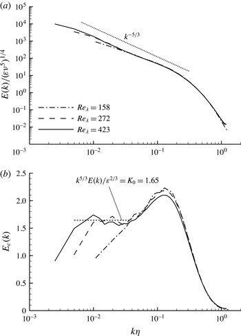
DNS results on energy spectra of homogeneous isotropic turbulence at three different Reynolds numbers: (a) energy spectra; (b) compensated energy spectra.

Before we conduct DNS and a priori LES analysis of the Euler angle and axis, the characteristics of DNS datasets need to be addressed. Detailed information on the input and output parameters for the three DNS datasets of homogeneous isotropic turbulence has been summarized in table 1. Here, we further examine the properties of the velocity field. Because there is no mean flow or mean shear stress in homogeneous isotropic turbulence, we focus our attention on the energy spectra obtained from DNS and validate the results against the K41 theory of Kolmogorov.
Figure 4 compares the energy spectra obtained from DNS at the three Reynolds numbers tested. According to the K41 theory of Kolmogorov on homogeneous isotropic turbulence, within the inertial subrange
 $1/l\ll k\ll 1/{\it\eta}$
, the energy spectra can be estimated using Kolmogorov’s well-known
 $-5/3$
law, i.e.
 $E(k)=K_{0}{\it\varepsilon}^{2/3}k^{-5/3}$
. Here,
 $K_{0}$
is a non-dimensional universal constant, namely, the Kolmogorov constant; and
 $l$
represents the integral length scale, defined as
 $$\begin{eqnarray}\displaystyle l=\frac{{\rm\pi}}{2u^{\prime 2}}\int _{0}^{k_{max}}\frac{E(k)}{k}\,\text{d}k. & & \displaystyle\end{eqnarray}$$
As shown in figure 4(a), the energy spectra for all three Reynolds numbers have a portion aligned with the dashed line (featuring the slope of
 $-5/3$
) in log–log coordinates around
 $k{\it\eta}=0.01$
. However, according to Kerr (Reference Kerr1990), Jiménez et al. (Reference Jiménez, Wray, Saffman and Rogallo1993) and Yeung & Zhou (Reference Yeung and Zhou1997), a more strict study of the TKE spectra against Kolmogorov’s
 $-5/3$
law can be performed using the compensated energy spectrum, defined as
 $E_{c}(k)\stackrel{\text{def}}{=}k^{5/3}{\it\varepsilon}^{-2/3}E(k)$
. As shown in figure 4(b), the ideal Kolmogorov spectra for the inertial subrange can be strictly represented using a horizontal dashed line. An obvious advantage of the compensated energy spectrum plot is that the value of
 $K_{0}$
can be precisely determined, as it is simply the ‘vertical height’ (value of
 $E_{c}(k)$
) of the horizontal dashed line.
The results shown in figure 4 are consistent with those of Ishihara, Gotoh & Kaneda (Reference Ishihara, Gotoh and Kaneda2009), who recently conducted a comprehensive review and concluded that the inertial subrange is not observed for
 $Re_{{\it\lambda}}\leqslant 200$
. Also, consistent with the DNS results of Ishihara et al. (Reference Ishihara, Gotoh and Kaneda2009), a narrow quasi-flat spectra region is observed at
 $k{\it\eta}\approx 0.01$
for
 $Re_{{\it\lambda}}=272$
, and this quasi-flat region becomes wider as the Reynolds number further increases to
 $Re_{{\it\lambda}}=423$
. From figure 4(b), it is clear that the Kolmogorov constant
 $K_{0}$
is approximately 1.65, which is close to the experimental value
 $K_{0}\approx 1.62$
(Sreenivasan Reference Sreenivasan1995) and DNS value
 $K_{0}=1.5{-}1.7$
(Yeung & Zhou Reference Yeung and Zhou1997; Gotoh & Fukayama Reference Gotoh and Fukayama2001; Kaneda et al.
Reference Kaneda, Ishihara, Yokokawa, Itakura and Uno2003). In comparison with figure 4(a), the compensated spectra shown in figure 4(b) indicate that the inertial subrange is apparently ‘shortened’. For the low Reynolds number
 $Re_{{\it\lambda}}=158$
, no significant inertial subrange can be observed from the compensated energy spectra.
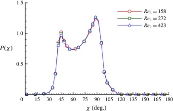
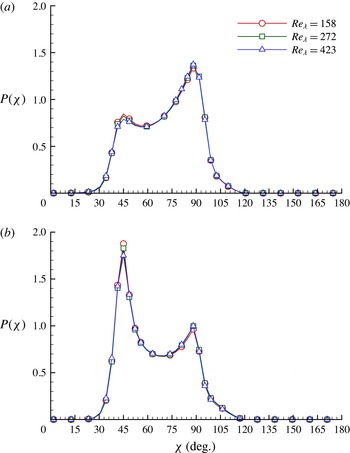
PDF of the Euler angle obtained from DNS at three Reynolds numbers.

Values of the mean Euler angle
 $\langle {\it\chi}\rangle$
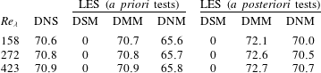
(deg.) predicted by DNS and different SGS stress models based on both a priori and a posteriori tests in the context of homogeneous isotropic turbulence at three Reynolds numbers.
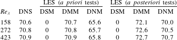
Table 2 compares the DNS and LES results on the mean Euler angle
 $\langle {\it\chi}\rangle$
for the three Reynolds numbers tested. Because the flow is homogeneous inside the entire computational domain, the value of
 $\langle {\it\chi}\rangle$
is unique for each Reynolds number. From table 2, it is interesting to observe that
 $\langle {\it\chi}\rangle$
is insensitive to the Reynolds number. The value of
 $\langle {\it\chi}\rangle$
is approximately
 $70.8^{\circ }$
for all three Reynolds numbers tested.
In order to refine the research, the probability density function (PDF) of the Euler angle is studied. The value of the Euler angle
 ${\it\chi}$
ranges from
 $0^{\circ }$
to
 $180^{\circ }$
, and 50 uniform bins have been used for calculating the statistics. Figure 5 compares the DNS results on the PDF
 $P({\it\chi})$
of the Euler angle for all three Reynolds numbers tested. From figure 5, it is clear that the curves of
 $P({\it\chi})$
for different Reynolds numbers collapse, indicating that the PDF of the instantaneous Euler angle is independent of the Reynolds number, which is consistent with the results on the mean Euler angle shown in table 2. Two modes are clearly observed in the profiles of
 $P({\it\chi})$
in figure 5. The primary mode occurs at
 ${\it\chi}=90^{\circ }$
, and the secondary one occurs at
 ${\it\chi}=45^{\circ }$
. In appendix A, based on a Taylor series approximation of the SGS stress tensor, we prove that these two special Euler angles,
 $90^{\circ }$
and
 $45^{\circ }$
, are consequences of the local instantaneous weak and strong shear conditions, respectively. It is proven in the appendix that, if the magnitude of a shear component is significantly smaller than those of the three normal components of the resolved velocity gradient tensor
 $\bar{\unicode[STIX]{x1D622}}_{ij}$
, then the state for
 ${\it\chi}=90^{\circ }$
is the most probable. On the other hand, if the magnitude of a shear component is significantly larger than those of the normal components, the Euler angle is
 $45^{\circ }$
identically.
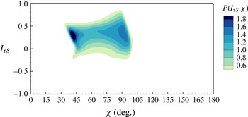
Contours of JPDF
 $P(I_{{\it\tau}S},{\it\chi})$
obtained from DNS at
 $Re_{{\it\lambda}}=423$
. Contours for low probability densities (
 $P(I_{{\it\tau}S},{\it\chi})<0.4$
) are clipped to highlight the most probable states.

It is interesting to observe from figure 5 that the PDF for
 ${\it\chi}=0^{\circ }$
is close to zero, which indicates that the eigenframe of
 $-{\it\tau}_{ij}^{d}$
is rarely in alignment with that of
 $\bar{\unicode[STIX]{x1D61A}}_{ij}$
. As demonstrated in Liu et al. (Reference Liu, Meneveau and Katz1994), the alignment between these two tensors can also be quantified using the following invariant,
 $$\begin{eqnarray}\displaystyle I_{{\it\tau}S}=\frac{-{\it\tau}_{ij}^{d}\bar{\unicode[STIX]{x1D61A}}_{ij}}{({\it\tau}_{kl}^{d}{\it\tau}_{kl}^{d})^{1/2}(\bar{S}_{mn}\bar{S}_{mn})^{1/2}}, & & \displaystyle\end{eqnarray}$$
which is the normalized form of the SGS dissipation rate
 ${\it\varepsilon}_{SGS}$
, and
 $I_{{\it\tau}S}\in [-1,1]$
holds. As such, it is expected that the instantaneous value of
 $I_{{\it\tau}S}$
can be either positive or negative, reflecting forward or backward scattering of KE. For a linear model (e.g. DSM), it is straightforward that
 $I_{{\it\tau}S}=\pm 1$
and
 ${\it\chi}=0^{\circ }$
. Figure 6 displays the contours of JPDF
 $P(I_{{\it\tau}S},{\it\chi})$
obtained from DNS at
 $Re_{{\it\lambda}}=423$
. The JPDF exhibits a bimodal pattern, with the primary mode located at
 $(I_{{\it\tau}S},{\it\chi})=(0.31,41^{\circ })$
and secondary mode located at
 $(0.46,91^{\circ })$
. The two preferred angles (
 $41^{\circ }$
and
 $91^{\circ }$
) observed in the JPDF are very close to the two modes (
 $45^{\circ }$
and
 $90^{\circ }$
) of the PDF of the Euler angle shown previously in figure 5 (corresponding to strong and weak shear conditions, respectively). Both forward scatter (for
 $I_{{\it\tau}S}>0$
) and backward scatter (for
 $I_{{\it\tau}S}<0$
) of KE are evident in figure 6. However, because the values of
 $I_{{\it\tau}S}$
for the two JPDF modes (0.31 and 0.46) are positive, the local KE flux is dominated by forward scatter from the filtered to the subgrid scales.
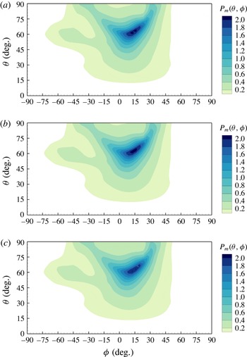
Contours of pre-multiplied JPDF
 $P_{m}({\it\theta},{\it\phi})$
obtained from DNS at three Reynolds numbers: (a)
 $Re_{{\it\lambda}}=158$
, (b)
 $Re_{{\it\lambda}}=272$
and (c)
 $Re_{{\it\lambda}}=423$
. Contours corresponding to low probability densities (
 $P_{m}({\it\theta},{\it\phi})<0.5$
) are clipped to highlight the most probable state.

In order to investigate the orientation of the Euler axis
 $\boldsymbol{q}$
, the contours of pre-multiplied JPDF
 $P_{m}({\it\theta},{\it\phi})$
obtained from DNS are demonstrated in figure 7. By comparing the contour patterns of the three Reynolds numbers exhibited in figure 7, it is evident that the orientation of the Euler axis
 $\boldsymbol{q}$
is insensitive to the Reynolds number. Particularly, the maximum of
 $P_{m}({\it\theta},{\it\phi})$
representing the most probable orientation of the Euler axis occurs at
 $({\it\theta},{\it\phi})=(62^{\circ },15^{\circ })$
for all three Reynolds numbers tested. Considering also the previous discussion of the Euler angle, it is interesting to note that the relative attitude between the eigenframes of
 $-{\it\tau}_{ij}^{d}$
and
 $\bar{\unicode[STIX]{x1D61A}}_{ij}$
(in terms of both the value of Euler angle
 ${\it\chi}$
and the orientation of Euler axis
 $\boldsymbol{q}$
) is independent of the Reynolds number.
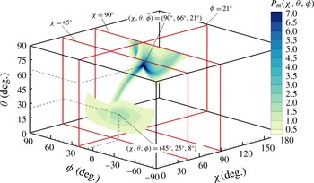
Contours of pre-multiplied JPDF
 $P_{m}({\it\chi},{\it\theta},{\it\phi})$
obtained from DNS at
 $Re_{{\it\lambda}}=423$
. Contours corresponding to low probability densities (
 $P_{m}({\it\chi},{\it\theta},{\it\phi})<0.5$
) are clipped to highlight the most probable state.

Thus far, the Euler angle
 ${\it\chi}$
and Euler axis
 $\boldsymbol{q}$
have been studied separately because they are both physically meaningful but mathematically independent parameters for the description of the eigenframe topology of the SGS stress tensor. In order to develop a general understanding of the attitude of the eigenframe of
 $-{\it\tau}_{ij}^{d}$
with respect to that of
 $\bar{\unicode[STIX]{x1D61A}}_{ij}$
, it is useful to further investigate the combined complete set of parameters
 $[{\it\chi},\boldsymbol{q}]$
, or specifically
 $[{\it\chi},{\it\theta},{\it\phi}]$
. Figure 8 displays the contours of the 3D pre-multiplied JPDF
 $P_{m}({\it\chi},{\it\theta},{\it\phi})\stackrel{\text{def}}{=}P({\it\chi},{\it\theta},{\it\phi})\sin {\it\theta}$
in plane
 ${\it\chi}=45^{\circ }$
,
 ${\it\chi}=90^{\circ }$
and
 ${\it\phi}=21^{\circ }$
obtained from DNS. Because the Euler angle and axis are independent of the Reynolds number, here we show only the DNS results for
 $Re_{{\it\lambda}}=423$
. It is demonstrated in figure 8 that the most probable state occurs at
 $({\it\chi},{\it\theta},{\it\phi})=(90^{\circ },66^{\circ },21^{\circ })$
. The Euler angle of this 3D mode (i.e.
 ${\it\chi}=90^{\circ }$
) is consistent with the most probable Euler angle observed in the PDF distribution in figure 5. However, the orientation of the Euler axis of this 3D mode (i.e.
 $({\it\theta},{\it\phi})=(66^{\circ },21^{\circ })$
) deviates slightly from the 2D mode (i.e.
 $({\it\theta},{\it\phi})=(62^{\circ },15^{\circ })$
) shown previously in figure 7(c). As discussed above, according to the PDF of the Euler angle exhibited in figure 5, there is a secondary mode of the Euler angle corresponding to
 ${\it\chi}=45^{\circ }$
. As is clear from figure 8, in the plane for
 ${\it\chi}=45^{\circ }$
, the most probable Euler axis is oriented at
 $({\it\theta},{\it\phi})=(25^{\circ },8^{\circ })$
. It is also interesting to observe the trends of the modes of these three independent quantities in figure 8. In the plane for
 ${\it\phi}=21^{\circ }$
, as the mode of the Euler angle
 ${\it\chi}$
varies from
 $45^{\circ }$
to
 $90^{\circ }$
, the mode of the colatitude
 ${\it\theta}$
increases steadily.
4.2 A priori test results
In a priori LES tests, the resolved strain rate tensor and model prediction of the SGS stress tensor are obtained by filtering the DNS data. The characteristics of the three DNS datasets on isotropic turbulence of three Reynolds numbers have been addressed previously in §§ 3.3 and 4.1. The a priori test results on the mean Euler angle
 $\langle {\it\chi}\rangle$
predicted by the three SGS stress models are compared against the DNS results in table 2. In sharp contrast to the DNS results, the value of
 $\langle {\it\chi}\rangle$
obtained from the DSM is
 $0^{\circ }$
identically. The reason that
 $\langle {\it\chi}\rangle \equiv 0^{\circ }$
holds strictly for the DSM lies in the fact that this model utilizes the conventional Boussinesq hypothesis and assumes a linear relationship between
 $-{\it\tau}_{ij}^{d}$
and
 $\bar{\unicode[STIX]{x1D61A}}_{ij}$
, i.e.
 $-{\it\tau}_{ij}^{d}\propto \bar{\unicode[STIX]{x1D61A}}_{ij}$
. This linear stress–strain relationship forces
 $\boldsymbol{E}^{-{\it\tau}}$
to be identical to
 $\boldsymbol{E}^{S}$
. Therefore, the DSM is characterized by the following unique condition:
 $$\begin{eqnarray}\displaystyle \unicode[STIX]{x1D64D}\equiv \boldsymbol{I},\quad {\it\chi}\equiv 0^{\circ }. & & \displaystyle\end{eqnarray}$$
As a result of this unique condition, the equation for determining the Euler axis
 $\boldsymbol{q}$
, i.e. (2.5), becomes singular, as its denominator (
 $2\sin {\it\chi}$
) becomes zero.
Owing to the inclusion of nonlinear components in their stress–strain modelling equations, both DMM and DNM are free from this singular condition characteristic of the DSM. As a result, the mean Euler angle predicted by the DMM and DNM is drastically different from that predicted by the DSM. As shown in table 2, the value of
 $\langle {\it\chi}\rangle$
predicted by the DMM is approximately
 $70.8^{\circ }$
for all three Reynolds numbers tested, which is in excellent agreement with the DNS results. The DNM also makes a reasonable prediction on the mean Euler angle; however, in comparison with the DNS data, it slightly underpredicts the mean Euler angle as approximately
 $65.7^{\circ }$
at all three Reynolds numbers tested. From the above discussion, an important conclusion can be obtained: the Euler angle and axis provide an effective criterion for quantitatively differentiating nonlinear and linear SGS models. For a linear model,
 ${\it\chi}\equiv 0^{\circ }$
and
 $\boldsymbol{q}$
is singular; whereas for a nonlinear model,
 ${\it\chi}\neq 0^{\circ }$
and
 $\boldsymbol{q}$
is well defined.
PDF of the Euler angle based on a priori tests of SGS stress models at three Reynolds numbers: (a) DMM and (b) DNM.

PDF of the Euler angle based on a priori tests of SGS stress models at
 $Re_{{\it\lambda}}=423$
.

The performance of SGS models in predicting the Euler angle can be further assessed based on the PDF of the Euler angle,
 $P({\it\chi})$
. Figure 9 compares the a priori test results of
 $P({\it\chi})$
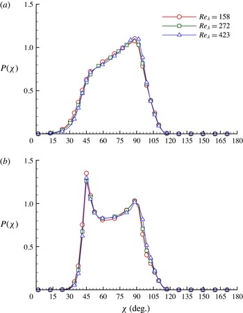
at three different Reynolds numbers. Because the Euler angle predicted by the DSM is identically zero, the PDF
 $P({\it\chi})$
for the DSM is known theoretically as a Dirac delta function at
 ${\it\chi}=0^{\circ }$
, viz.
 $P({\it\chi})={\it\delta}(0^{\circ })$
. Therefore, only results predicted by the DMM and DNM need to be shown in figure 9. As demonstrated in figure 9, the probability densities of the instantaneous Euler angle
 ${\it\chi}$
predicted by both DMM and DNM are independent of the Reynolds number. This observation is consistent with the conclusion on the mean Euler angle
 $\langle {\it\chi}\rangle$
based on the previous analysis of table 2.
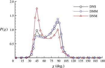
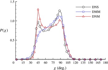
Figure 10 compares the a priori test results of
 $P({\it\chi})$
predicted by the DMM and DNM against the DNS results. Because the Euler angle is insensitive to the Reynolds number, only the results for
 $Re_{{\it\lambda}}=423$
are presented. From figure 10, it is clear that the primary mode for
 ${\it\chi}=90^{\circ }$
is well predicted by the DMM. The secondary mode for
 ${\it\chi}=45^{\circ }$
can also be observed from the result of the DMM, but the magnitude of this mode is slightly underpredicted. The characteristic bimodal shape of
 $P({\it\chi})$
is qualitatively captured by the DNM. As demonstrated in figure 10, the two modes predicted by the DNM are also located at
 ${\it\chi}=45^{\circ }$
and
 $90^{\circ }$
, which are consistent with the DNS results. However, the DNM incorrectly predicts state
 ${\it\chi}=45^{\circ }$
as the primary mode. This explains the previous observation that, in comparison with the DNS results, the mean Euler angle is underpredicted by the DNM (see table 2).
Contours of pre-multiplied JPDF
 $P_{m}({\it\theta},{\it\phi})$
at
 $Re_{{\it\lambda}}=423$
based on a priori tests of SGS stress models: (a) DMM and (b) DNM. Contours corresponding to low probability densities (
 $P_{m}({\it\theta},{\it\phi})<0.5$
) are clipped to highlight the most probable state.

In sharp contrast to the performance of the DSM, as shown in figure 10, the probability density for the state of
 ${\it\chi}=0^{\circ }$
is zero for both DMM and DNM, indicating that the Euler axis can be well determined through (2.5) for these two nonlinear models. In order to study the orientation of the Euler axis, the a priori test results of
 $P_{m}({\it\theta},{\it\phi})$
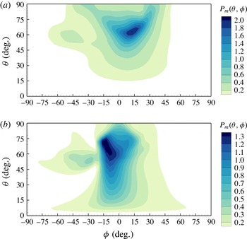
predicted by the DMM and DNM are compared in figure 11. As shown in figure 11(b), the most probable orientation of the Euler axis predicted by the DNM occurs approximately at
 $({\it\theta},{\it\phi})=(72^{\circ },-10^{\circ })$
, which is different from DNS results shown in figure 7(c) and the prediction of the DMM shown in figure 11(a). Furthermore, a secondary mode is observed in figure 11(b) at
 $({\it\theta},{\it\phi})=(52^{\circ },-30^{\circ })$
, which does not agree with the DNS results. The a priori test results indicate that, although the DNM does a reasonable job on the prediction of the mean and instantaneous values of the Euler angle, its ability to predict the orientation of the Euler axis is limited.
4.3 A posteriori test results
Different from an a priori test, an a posteriori test evaluates the performance of an SGS stress model by incorporating it in a numerical simulation and then validating the obtained LES results against experimental or DNS data. Although both a priori and a posteriori tests are important approaches for SGS model testing, and both can be found widely in the literature, the conclusions on the performance of the same SGS model from these two LES approaches can sometimes be drastically different. These two LES approaches are conceptually different in many subtle ways in terms of their testing procedures and filtering processes at grid and test-grid levels, and fully consistent diagnoses of a deterministic SGS stress model from both a priori and a posteriori tests can be very challenging due to the stochastic nature of SGS stresses (see e.g. Park, Yoo & Choi (Reference Park, Yoo and Choi2005) and many other papers on the efficacy of these two LES methods). However, there are exceptions. In their research, Chen et al. (Reference Chen, Zhang, Wang and Tong2003) derived the transport equation of the conditional averaged JPDF of instantaneous velocity fluctuations, which provides an effective method for assessing the relationship between resolved velocity and the SGS dissipation rate. This method was later used by Chen et al. (Reference Chen, Zhang, Wang and Tong2003) and Chen & Tong (Reference Chen and Tong2006) to perform a priori tests, and by Chen et al. (Reference Chen, Otte, Sullivan and Tong2009) to perform a posteriori tests. Their a priori and a posteriori test results on the averaged SGS dissipation rate conditioned by the resolved velocity are highly consistent. Nevertheless, in order to conduct a comprehensive comparative study to draw fair conclusions, here we further test the eigenframe topology of the SGS stress tensor based on the same three SGS models using the a posteriori approach at three Reynolds numbers.
In table 2, the a posteriori test results on the mean Euler angle
 $\langle {\it\chi}\rangle$
are compared against the DNS and a priori test results. Similar to the a priori tests, the values of
 $\langle {\it\chi}\rangle$
predicted by all three SGS models are insensitive to the Reynolds number in the a posteriori tests. The value of
 $\langle {\it\chi}\rangle$
predicted by the DMM is approximately
 $72.4^{\circ }$
, which is slightly larger than the DNS value. From this point of view, the predictive performance of the DMM in the a posteriori test is not as good as that in the a priori test. The a posteriori prediction of the mean Euler angle
 $\langle {\it\chi}\rangle$
by the DNM is approximately
 $70.4^{\circ }$
, which is in excellent agreement with the DNS result. From table 2, it is clear that the predictive performance of the DNM is significantly better in an a posteriori test than in an a priori test. Obviously, this trend is opposite to the performance of the DMM discussed above. Figure 12 compares the PDF of the Euler angle based on a posteriori tests of SGS stress models at three Reynolds numbers. By comparing figure 12 with figure 9, it is clear that the model predictions of the PDF of
 ${\it\chi}$
are similar in the a priori and a posteriori approaches. As is evident from figure 12, the distributions of
 $P({\it\chi})$
predicted by DMM and DNM in a posteriori tests are also insensitive to the Reynolds number, an observation which is consistent with the previous conclusion on the mean Euler angle value
 $\langle {\it\chi}\rangle$
obtained from table 2.
PDF of the Euler angle based on a posteriori tests of SGS stress models at three Reynolds numbers: (a) DMM and (b) DNM.

PDF of the Euler angle based on a posteriori tests of SGS stress models at
 $Re_{{\it\lambda}}=423$
.

Figure 13 compares the a posteriori test results on the PDF of the Euler angle obtained using different SGS stress models. Because the Euler angle is independent of the Reynolds number, here we only display the results for
 $Re_{{\it\lambda}}=423$
. From figure 13, it is observed that, in comparison with the DNS results, the bimodal shape of
 $P({\it\chi})$
is not fully reproduced by the DMM, as it almost misses the prediction of the secondary mode for
 ${\it\chi}=45^{\circ }$
. On the other hand, the DMM slightly overpredicts
 $P({\it\chi})$
for
 $100^{\circ }\leqslant {\it\chi}\leqslant 120^{\circ }$
. This well explains the observation that the DMM slightly overpredicts the mean value of the Euler angle in a posteriori tests (see table 2). The DNM successfully captures the bimodal pattern of
 $P({\it\chi})$
with two modes located at
 ${\it\chi}=45^{\circ }$
and
 $90^{\circ }$
. Consistent with the previous a priori test results shown in figure 10, the primary mode predicted by the DNM in the a posteriori test also corresponds to
 ${\it\chi}=45^{\circ }$
, which, however, deviates from the DNS result (see figure 5). Similar to the behaviour of the DMM, the DNM also slightly overpredicts
 $P({\it\chi})$
for
 $100^{\circ }\leqslant {\it\chi}\leqslant 120^{\circ }$
.
Contours of pre-multiplied JPDF
 $P_{m}({\it\theta},{\it\phi})$
based on a posteriori tests of SGS stress models at
 $Re_{{\it\lambda}}=423$
: (a) DMM and (b) DNM. Contours corresponding to low probability densities (
 $P_{m}({\it\theta},{\it\phi})<0.5$
) are clipped to highlight the most probable state.

In order to investigate the SGS modelling effects on the orientation of the Euler axis, the a posteriori test results of
 $P_{m}({\it\theta},{\it\phi})$
predicted using the DMM and DNM for
 $Re_{{\it\lambda}}=423$
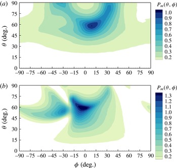
are compared in figure 14. The a posteriori results shown can be validated against the DNS result for the same Reynolds number presented previously in figure 7(c). As shown in figure 14(a), the mode of
 $P_{m}({\it\theta},{\it\phi})$
predicted by the DMM occurs at approximately
 $({\it\theta},{\it\phi})=(60^{\circ },13^{\circ })$
, which is in good agreement with the most probable state obtained from DNS, i.e.
 $({\it\theta},{\it\phi})=(62^{\circ },15^{\circ })$
. However, the JPDF value of this mode is underpredicted by the DMM, and, as a result, the pre-multiplied JPDF of
 $({\it\theta},{\it\phi})$
in the model prediction (shown in figure 14
a) has a broader distribution than that of the DNS result (shown in figure 7
c). Furthermore, by comparing figure 14(a) with figures 11(a) and 7(c), it is clear that the a priori test outperforms the a posteriori test in terms of the prediction of the orientation of the Euler axis.
Figure 14(b) displays the a posteriori test results of
 $P_{m}({\it\theta},{\it\phi})$
obtained using the DNM, which shows that the most probable state of the Euler axis orientation occurs at
 $({\it\theta},{\it\phi})\approx (60^{\circ },-4^{\circ })$
. Although the colatitude
 ${\it\theta}$
of this mode agrees well with the DNS result, the predicted longitude
 ${\it\phi}$
is not accurate. Similar to the a priori test result shown in figure 11(b), a secondary mode is observed at
 $({\it\theta},{\it\phi})=(54^{\circ },-30^{\circ })$
, which, however, is not evidenced by DNS.
5 Conclusions
The topology of the eigenframe of the SGS stress tensor is systematically studied using the proposed Euler angle and axis method. In order to study the geometrical properties of the eigenframes of
 $-{\it\tau}_{ij}^{d}$
and
 $\bar{\unicode[STIX]{x1D61A}}_{ij}$
, a deterministic procedure is proposed to eliminate any ambiguities involved in the topology of eigenframes. Both Euler angle and axis are natural invariants of the rotation matrix
 $\unicode[STIX]{x1D64D}$
between the eigenframes of
 $-{\it\tau}_{ij}^{d}$
and
 $\bar{\unicode[STIX]{x1D61A}}_{ij}$
, which are unique in mathematical representations and provide an elegant and effective approach for describing the eigenframe topology of the SGS stress tensor. In order to validate the theory, three conventional dynamic SGS stress models are tested in the context of homogenous isotropic turbulence using both a priori and a posteriori approaches, and the LES predictions are thoroughly compared against the DNS and analytical results.
An important conclusion of this research is that the Euler angle and axis can provide an effective criterion for quantitatively differentiating nonlinear and linear SGS models: for a linear model,
 $\unicode[STIX]{x1D64D}\equiv \boldsymbol{I}$
,
 ${\it\chi}\equiv 0^{\circ }$
and
 $\boldsymbol{q}$
is singular; whereas for a nonlinear model,
 ${\it\chi}\neq 0^{\circ }$
and
 $\boldsymbol{q}$
is well defined. The DSM has been very successful in numerous applications since its invention, because it ensures a net positive SGS dissipation rate from the filtered to the subgrid scales. The success of the Smagorinsky-type models lies in the direct projection of the SGS stress tensor onto the resolved strain rate tensor in a linear manner based on the Boussinesq assumption. However, owing to the same reason for its success, the DSM, on the other hand, totally fails to reproduce the correct eigenframe topology of the SGS tensor. In contrast, due to the inclusion of the nonlinear components in their modelling formulations, the predictive performances of the DMM and DNM enhance drastically in both a priori and a posteriori tests.
The mean Euler angle
 $\langle {\it\chi}\rangle$
predicted by DNS is approximately
 $70.8^{\circ }$
for all three Reynolds numbers tested. The PDF of the Euler angle
 $P({\it\chi})$
forms a bimodal shape, with the primary and secondary modes at
 ${\it\chi}=90^{\circ }$
and
 $45^{\circ }$
, respectively. Based on a Taylor series expansion of the SGS stress tensor with respect to the filter size, it is proven analytically that these two preferred Euler angles (i.e.
 $90^{\circ }$
and
 $45^{\circ }$
) are in effect direct consequences of local instantaneous weak and strong shear conditions, respectively. To quantify the orientation of Euler axis
 $\boldsymbol{q}$
, its colatitude
 ${\it\theta}$
and longitude
 ${\it\phi}$
are considered. By analysing the DNS results of the pre-multiplied JPDF of
 ${\it\theta}$
and
 ${\it\phi}$
, it is observed that the most probable Euler axis orientation occurs at
 $({\it\theta},{\it\phi})=(62^{\circ },15^{\circ })$
.
Both a priori and a posteriori test results indicate that the Euler angle and axis predicted by all three SGS stress models are Reynolds-number-independent, an observation which is consistent with the DNS results. Both Euler angle and Euler axis predicted by the DMM are in excellent agreement with the DNS results in the a priori tests. In the a posteriori tests, the DMM underperforms in terms of the prediction of the Euler angle
 ${\it\chi}$
. Numerical simulations based on the DMM almost miss the prediction of the secondary mode (
 ${\it\chi}=45^{\circ }$
) in the distribution of
 $P({\it\chi})$
. Furthermore, it is clear that, for the DMM, the a priori test outperforms the a posteriori test in terms of the prediction of the orientation of the Euler axis. Specifically, the pre-multiplied JPDF
 $P_{m}({\it\theta},{\it\phi})$
predicted by the DMM in a posteriori tests exhibits a broader distribution than the DNS results.
The mean Euler angle predicted by the DNM is approximately
 $65.7^{\circ }$
based on a priori tests, which is smaller than the DNS value. In both a priori and a posteriori tests, the DNM successfully captures the bimodal shape of the PDF of the Euler angle; however, it misdiagnoses the secondary mode as the primary mode, and consequently it predicts the most probable value of the Euler angle to be
 ${\it\chi}=45^{\circ }$
. The mean Euler angle
 $\langle {\it\chi}\rangle$
predicted by the DNM is approximately
 $70.4^{\circ }$
in the a posteriori test, which is slightly better than that obtained in the a priori test in comparison with the DNS value. The most probable orientation of the Euler axis predicted by the DNM deviates from the DNS result in both a priori and a posteriori tests, indicating that the geometrical properties of the SGS stress tensor as represented by the DNM formulation are still limited. It should be indicated that the statistical results of the Euler angle and axis presented in this study can sometimes be different between the a priori and a posteriori approaches. To further refine this comparative study, it would be interesting to examine whether the agreement between these two LES approaches can be improved if the calculations of statistics of the Euler angle and axis are conditioned with the resolved-scale velocity by following the approach of Chen & Tong (Reference Chen and Tong2006) and Chen et al. (Reference Chen, Otte, Sullivan and Tong2009).
It should also be indicated that the numerical tests conducted in this research based on DNS and LES are limited to three low and moderate Reynolds numbers ranging from
 $Re_{{\it\lambda}}=158$
to 423. In future studies, it would be beneficial to further test the proposed theory at higher Reynolds numbers. Besides the discrete box filter tested in the present study, it would be interesting to investigate the effects of filter types on the predicted eigenframe topology of the SGS stress tensor (by comparing the current results against those obtained based on, for example, discrete Gaussian and sharp spectral cut-off filters) in a priori and a posteriori approaches. As such, it would be possible to further clarify, for example, if the excellent predictive performance of the DMM observed in the current a priori tests is independent of filter types.
Finally, through this study, it becomes clear that all three SGS stress models tested have certain weaknesses in terms of their prediction of the eigenframe topology of the SGS stress tensor. This indicates that their modelling formulations have some intrinsic shortcomings and there is room for potential new modifications to these SGS stress models in order to further improve their predictive capability. In traditional SGS model testing, a model is often assessed with respect to its capability to predict statistical moments, coherent structures and energy spectra of the resolved flow field. The current study focuses instead on fine tensorial geometrical properties of the SGS stress tensor and fundamentals of the stress–strain equations. It should be indicated that both the traditional and current focuses on SGS model testing are important; it is just that their criteria are different. In future studies, it is possible to extend the evaluation of a new SGS model to include also consideration of its predictive accuracy on the eigenframe topology of the SGS stress tensor (based on new criteria such as that the Euler angle is expected to be around
 $70^{\circ }$
in isotropic turbulence at low and moderate Reynolds numbers). As such, a more comprehensive understanding of the SGS stress tensor may be developed from different angles, in terms of not only the primitive need of an SGS stress model for closure of governing equations to compute flow statistics but also the desire for an in-depth knowledge of the tensorial geometrical properties of the stress–strain relationship and eigenframe topology of the SGS tensor itself.
Acknowledgements
The authors would like to thank Western Canada Research Grid (WestGrid) for access to supercomputing facilities. Research funding from the Natural Sciences and Engineering Research Council (NSERC) of Canada to B.-C.W. is gratefully acknowledged.
Appendix A. Sufficient conditions for the most probable Euler angle
In § 4.1, the PDF of the Euler angle
 $P({\it\chi})$
predicted by DNS forms a bimodal pattern, with the primary and secondary modes being
 ${\it\chi}=90^{\circ }$
and
 $45^{\circ }$
, respectively. In this appendix, we further prove that these two special Euler angles correspond to local weak and strong shear conditions, respectively. To demonstrate, the SGS stress tensor is first approximated using its Taylor series expansion with respect to the filter size
 $\bar{{\it\Delta}}$
following the approach of Liu et al. (Reference Liu, Meneveau and Katz1994), viz.
 $$\begin{eqnarray}\displaystyle {\it\tau}_{ij}={\textstyle \frac{1}{12}}\bar{{\it\Delta}}^{2}\bar{\unicode[STIX]{x1D622}}_{ik}\bar{\unicode[STIX]{x1D622}}_{jk}+O(\bar{{\it\Delta}}^{4}), & & \displaystyle\end{eqnarray}$$
where
 $\bar{\unicode[STIX]{x1D622}}_{ij}=\partial \bar{u}_{i}/\partial x_{j}$
represents the resolved velocity gradient tensor. With the above approximation, once
 $\bar{\unicode[STIX]{x1D622}}_{ij}$
is obtained, both
 ${\it\tau}_{ij}$
and
 $\bar{\unicode[STIX]{x1D61A}}_{ij}$
are determined, and furthermore the Euler angle can be calculated analytically. In order to make clear the procedure for calculating the Euler angle, we preprocess
 $\bar{\unicode[STIX]{x1D622}}_{ij}$
using the following two steps.
Step 1. Use an orthonormal transformation
 $\bar{\unicode[STIX]{x1D656}}=\unicode[STIX]{x1D64C}\,\bar{\unicode[STIX]{x1D656}}^{(0)}\unicode[STIX]{x1D64C}^{\text{T}}$
to sort the diagonal components of
 $\bar{\unicode[STIX]{x1D622}}_{ij}$
in descending order of their absolute values, i.e.
 $|\bar{\unicode[STIX]{x1D622}}_{11}|\geqslant |\bar{\unicode[STIX]{x1D622}}_{22}|\geqslant |\bar{\unicode[STIX]{x1D622}}_{33}|$
. Here,
 $\bar{\unicode[STIX]{x1D656}}^{(0)}$
and
 $\bar{\unicode[STIX]{x1D656}}$
represent the resolved velocity gradient tensor before and after the preprocessing, respectively. This step can always be achieved by properly choosing an orthogonal matrix
 $\unicode[STIX]{x1D64C}$
. Because the Euler angle is an invariant between
 $-{\it\tau}_{ij}^{d}$
and
 $\bar{\unicode[STIX]{x1D61A}}_{ij}$
, the above orthonormal transformation does not alter its value.
Step 2. Normalize
 $\bar{\unicode[STIX]{x1D622}}_{ij}$
obtained from step 1 using
 $\bar{\unicode[STIX]{x1D622}}_{11}$
. Although this normalization process alters the magnitudes of
 $-{\it\tau}_{ij}^{d}$
and
 $\bar{\unicode[STIX]{x1D61A}}_{ij}$
, their eigenframes are not affected.
The goal of the following analysis is to find the theoretical explanation for the two modes
 ${\it\chi}=45^{\circ }$
and
 ${\it\chi}=90^{\circ }$
in the PDF distribution of the Euler angle observed in the DNS and LES studies. To find necessary conditions for these two modes is overly ambitious, as it demands full knowledge of all possible states of the instantaneous velocity gradient tensor in the context of isotropic turbulence. To achieve our goal of analysis, we need to restrict our ambition to findings of sufficient conditions for these two modes.
After preprocessing
 $\bar{\unicode[STIX]{x1D622}}_{ij}$
following the above two steps, we now consider a special condition with only one shear component of
 $\bar{\unicode[STIX]{x1D622}}_{ij}$
being non-trivial. For an incompressible fluid, the instantaneous resolved velocity gradient tensor can then be parametrized using an arbitrary shear component
 $a$
and an arbitrary normal component
 $b$
as
 $$\begin{eqnarray}\displaystyle \bar{\unicode[STIX]{x1D622}}_{ij}=\left[\begin{array}{@{}ccc@{}}1 & a & 0\\ 0 & -b & 0\\ 0 & 0 & b-1\end{array}\right]. & & \displaystyle\end{eqnarray}$$
Because the diagonal components of
 $\bar{\unicode[STIX]{x1D622}}_{ij}$
have been sorted in descending order in accordance with their absolute values, the following restriction on the value of
 $b$
holds:
 $$\begin{eqnarray}\displaystyle 0.5<b<1. & & \displaystyle\end{eqnarray}$$
In (A 2), we assume
 $\bar{\unicode[STIX]{x1D622}}_{12}=a$
. This is an arbitrary choice, because other shear components (
 $\bar{\unicode[STIX]{x1D622}}_{13}$
,
 $\bar{\unicode[STIX]{x1D622}}_{21}$
,
 $\bar{\unicode[STIX]{x1D622}}_{23}$
,
 $\bar{\unicode[STIX]{x1D622}}_{31}$
or
 $\bar{\unicode[STIX]{x1D622}}_{32}$
) may also be assumed as the only non-trivial shear component with a value of
 $a$
. The procedure for calculating the Euler angle is very similar in these alternative cases, and all these alternative cases actually result in the same value of the Euler angle (as long as there is only one non-trivial shear component). In view of this, in order to keep the derivations concise, here we only present the analysis based on (A 2). From (A 2), the resolved strain rate tensor
 $\bar{\unicode[STIX]{x1D61A}}_{ij}=(\bar{\unicode[STIX]{x1D622}}_{ij}+\bar{\unicode[STIX]{x1D622}}_{ji})/2$
can be readily calculated, viz.
 $$\begin{eqnarray}\displaystyle \bar{\unicode[STIX]{x1D61A}}_{ij}=\left[\begin{array}{@{}ccc@{}}1 & a/2 & 0\\ a/2 & -b & 0\\ 0 & 0 & b-1\end{array}\right], & & \displaystyle\end{eqnarray}$$
and from (A 1), the trace-free SGS stress tensor is estimated as
 $$\begin{eqnarray}\displaystyle -{\it\tau}_{ij}^{d}=-\frac{\bar{{\it\Delta}}^{2}}{36}\left[\begin{array}{@{}ccc@{}}-2b^{2}+2b+1+2a^{2} & -3ab & 0\\ -3ab & b^{2}+2b-2-a^{2} & 0\\ 0 & 0 & b^{2}-4b+1-a^{2}\end{array}\right]. & & \displaystyle\end{eqnarray}$$
With the above two equations for
 $\bar{\unicode[STIX]{x1D61A}}_{ij}$
and
 $-{\it\tau}_{ij}^{d}$
, the Euler angles for weak (
 $|a|\ll 1-b<b<1$
) and strong (
 $|a|\gg 1>b>1-b$
) shear conditions can be determined as follows.
(1) Weak shear condition for
 $|a|\ll 1-b<b<1$
Under the weak shear condition, by neglecting the shear components
 $a/2$
in (A 4), the eigenframe of
 $\bar{\unicode[STIX]{x1D61A}}_{ij}$
can be obtained as
 $$\begin{eqnarray}\displaystyle \boldsymbol{E}^{S}=\left[\begin{array}{@{}ccc@{}}1 & 0 & 0\\ 0 & 1 & 0\\ 0 & 0 & 1\end{array}\right]. & & \displaystyle\end{eqnarray}$$
Using the condition
 $|a|\ll 1-b<b<1$
, the trace-free SGS stress tensor given by (A 5) can be simplified to
 $$\begin{eqnarray}\displaystyle -{\it\tau}_{ij}^{d}\approx \frac{\bar{{\it\Delta}}^{2}}{36}\left[\begin{array}{@{}ccc@{}}{\it\Lambda}_{{\it\alpha}} & 0 & 0\\ 0 & {\it\Lambda}_{{\it\beta}} & 0\\ 0 & 0 & {\it\Lambda}_{{\it\gamma}}\end{array}\right], & & \displaystyle\end{eqnarray}$$
where
 ${\it\Lambda}_{{\it\alpha}}=2b^{2}-2b-1$
,
 ${\it\Lambda}_{{\it\beta}}=-b^{2}-2b+2$
and
 ${\it\Lambda}_{{\it\gamma}}=-b^{2}+4b-1$
. Given the restriction
 $0.5<b<1$
, it can be shown that
 $$\begin{eqnarray}\displaystyle \left.\begin{array}{@{}c@{}}|{\it\Lambda}_{{\it\alpha}}|>|{\it\Lambda}_{{\it\gamma}}|>|{\it\Lambda}_{{\it\beta}}|\quad (\text{if }0.5<b<\sqrt{3}-1),\\ |{\it\Lambda}_{{\it\gamma}}|>|{\it\Lambda}_{{\it\alpha}}|>|{\it\Lambda}_{{\it\beta}}|\quad (\text{if }\sqrt{3}-1<b<1).\end{array}\right\} & & \displaystyle\end{eqnarray}$$
Under the first of the above two conditions (for
 $0.5<b<\sqrt{3}-1$
), the eigenframe of
 $-{\it\tau}_{ij}^{d}$
reads
 $$\begin{eqnarray}\displaystyle \boldsymbol{E}^{-{\it\tau}}=\left[\begin{array}{@{}ccc@{}}1 & 0 & 0\\ 0 & 0 & -1\\ 0 & 1 & 0\end{array}\right]. & & \displaystyle\end{eqnarray}$$
From (2.3), the rotation matrix between the eigenframes of
 $\bar{\unicode[STIX]{x1D61A}}_{ij}$
and
 $-{\it\tau}_{ij}^{d}$
can be calculated, viz.
 $$\begin{eqnarray}\displaystyle \unicode[STIX]{x1D64D}=\boldsymbol{E}^{-{\it\tau}}(\boldsymbol{E}^{S})^{\text{T}}=\left[\begin{array}{@{}ccc@{}}1 & 0 & 0\\ 0 & 0 & -1\\ 0 & 1 & 0\end{array}\right], & & \displaystyle\end{eqnarray}$$
and as a result, the value of the Euler angle can be determined using (2.4) as
 $$\begin{eqnarray}\displaystyle {\it\chi}=\arccos \frac{\text{tr}(\unicode[STIX]{x1D64D})-1}{2}=\arccos (0)=90^{\circ }. & & \displaystyle\end{eqnarray}$$
Under the second of the two conditions given by (A 8), it can be demonstrated that the rotation matrix becomes
 $$\begin{eqnarray}\displaystyle \unicode[STIX]{x1D64D}=\left[\begin{array}{@{}ccc@{}}0 & 1 & 0\\ 0 & 0 & 1\\ 1 & 0 & 0\end{array}\right], & & \displaystyle\end{eqnarray}$$
and the Euler angle corresponding to the above rotation matrix is
 $$\begin{eqnarray}\displaystyle {\it\chi}=\arccos \frac{\text{tr}(\unicode[STIX]{x1D64D})-1}{2}=\arccos \left(-\frac{1}{2}\right)=120^{\circ }. & & \displaystyle\end{eqnarray}$$
In summary, under the weak shear condition for
 $|a|\ll 1-b<b<1$
, as long as there is one and only one non-trivial shear component in the instantaneous velocity gradient tensor, the Euler angle must be either
 $90^{\circ }$
(if
 $0.5<b<\sqrt{3}-1$
) or
 $120^{\circ }$
(if
 $\sqrt{3}-1<b<1$
).


The above conclusion on the Euler angle under the weak shear condition
 $|a|\ll 1-b<b<1$
is obtained based on the assumption that shear rate
 $a$
is negligible. In order to understand the influence of
 $a$
on the value of the Euler angle, (A 4) and (A 5) can be directly used. Figure 15 demonstrates the asymptotic behaviour of the Euler angle in response to different values of
 $a$
. As shown in figure 15, under a very weak shear rate for
 $a=0.001$
, the value of the Euler angle jumps sharply from
 $90^{\circ }$
to
 $120^{\circ }$
at the critical point for
 $b=\sqrt{3}-1\approx 0.732$
, which is fully consistent with the analytical results obtained above. Also it is interesting to observe that, for
 $a=0.001$
, the Euler angle drops sharply from
 ${\it\chi}=120^{\circ }$
when
 $b\rightarrow 1$
. This is because the weak shear condition
 $|a|\ll 1-b$
is no longer valid. As is evident in figure 15, the Euler angle strictly equals
 $90^{\circ }$
if
 $0.5<b<\sqrt{3}-1$
(i.e. under the first condition in (A 8)) regardless of the value of
 $a$
; however, its value deviates from
 $120^{\circ }$
if
 $\sqrt{3}-1<b<1$
(i.e. under the second condition in (A 8)) as the value of
 $a$
increases. This is consistent with the DNS result (see figure 5) that
 ${\it\chi}=90^{\circ }$
is the most probable Euler angle in homogeneous isotropic turbulence, whereas the probability density for the state of
 ${\it\chi}=120^{\circ }$
is negligible (because this state occurs only when that value of
 $a$
is extremely small).
(2) Strong shear condition for
 $|a|\gg 1>b>1-b$
By neglecting the diagonal components of
 $\bar{\unicode[STIX]{x1D61A}}_{ij}$
, it can be proven that the eigenframe of
 $\bar{\unicode[STIX]{x1D61A}}_{ij}$
becomes
 $$\begin{eqnarray}\displaystyle \boldsymbol{E}^{S}=\left[\begin{array}{@{}ccc@{}}\sqrt{2}/2 & -\sqrt{2}/2 & 0\\ \sqrt{2}/2 & \sqrt{2}/2 & 0\\ 0 & 0 & 1\end{array}\right]. & & \displaystyle\end{eqnarray}$$
By applying the strong shear condition to (A 5), the eigenvalues of
 $-{\it\tau}_{ij}^{d}$
can be obtained as
 $$\begin{eqnarray}\displaystyle \left.\begin{array}{@{}c@{}}{\it\lambda}_{1}^{-{\it\tau}}=-\displaystyle \frac{\bar{{\it\Delta}}^{2}(a^{2}+a\sqrt{9a^{2}+36b^{2}})}{72}\approx -\displaystyle \frac{\bar{{\it\Delta}}^{2}a^{2}}{18},\\ {\it\lambda}_{2}^{-{\it\tau}}=-\displaystyle \frac{\bar{{\it\Delta}}^{2}(a^{2}-a\sqrt{9a^{2}+36b^{2}})}{72}\approx \displaystyle \frac{\bar{{\it\Delta}}^{2}a^{2}}{36},\\ {\it\lambda}_{3}^{-{\it\tau}}=\displaystyle \frac{\bar{{\it\Delta}}^{2}a^{2}}{36},\end{array}\right\} & & \displaystyle\end{eqnarray}$$
and the eigenframe of
 $-{\it\tau}_{ij}^{d}$
reads
 $$\begin{eqnarray}\displaystyle \boldsymbol{E}^{-{\it\tau}}=\left[\begin{array}{@{}ccc@{}}1 & 0 & 0\\ 0 & 1 & 0\\ 0 & 0 & 1\end{array}\right]. & & \displaystyle\end{eqnarray}$$
The rotation matrix is then obtained as
 $$\begin{eqnarray}\displaystyle \unicode[STIX]{x1D64D}=\left[\begin{array}{@{}ccc@{}}\sqrt{2}/2 & \sqrt{2}/2 & 0\\ -\sqrt{2}/2 & \sqrt{2}/2 & 0\\ 0 & 0 & 1\end{array}\right], & & \displaystyle\end{eqnarray}$$
and subsequently, the value of the Euler angle can be calculated as
 $$\begin{eqnarray}\displaystyle {\it\chi}=\arccos \frac{\mathtt{tr}(\unicode[STIX]{x1D64D})-1}{2}=\arccos \left(\frac{\sqrt{2}}{2}\right)=45^{\circ }. & & \displaystyle\end{eqnarray}$$
This concludes that
 ${\it\chi}=45^{\circ }$
holds under the strong shear condition for
 $|a|\gg 1>b>1-b$
.