3.1.1. Connection between wave potentials

Consider the connection between the wave potentials $\psi _j(x,y), \,j=1,2$ , and the new auxiliary wave potentials $\chi _j(x,y), \,j=1,2$ , as given by (see Mondal et al. Reference Mondal, Ashok and Manam2024)

(3.5) \begin{align} \left [\frac {\partial ^4}{\partial y^4} - \beta ^2\right ]\psi _j(x,y)+ \textrm {i} m_1 \Gamma \displaystyle \int _{0}^{x}\frac {\partial ^4 }{\partial y^4} \sigma _j(t, y)\,{\rm d}t +\beta ^2 \left (\frac {\rho }{m_p}- \textrm {i} m_1 \Gamma \right ) \displaystyle \int _{0}^{x} \sigma _j(t, y) {\rm d}t \nonumber \\ = \chi _j(x,y), (-1)^{j+1}x\gt 0, \quad j=1,2, \end{align}

where $ \sigma _j(t, y)= \sum _{i=1}^{2} \left \{ ( e^{-\textrm {i} \mu _i t} + e^{\textrm {i} \mu _i t} ) g_0(m_i,y) + \psi _i((-1)^{j+i} t, y) \right \}$ and the involved auxiliary wave potentials $\chi _j(x,y), j=1,2$ , satisfy (2.1)–(2.5). All the terms in the above well-defined connection (3.5) carry out the modified Helmholtz equation (2.1). The above integro-differential relation (3.5) is differentiated with respect to $x$ , we obtain that

(3.6) \begin{align} \left [\frac {\partial ^4}{\partial y^4} - \beta ^2 \right ] \psi _{jx}(x,y)+ \textrm {i} m_1 \Gamma \, \frac {\partial ^4 }{\partial y^4} \sigma _j(x, y) +\beta ^2 \left (\frac {\rho }{m_p}- \textrm {i} m_1 \Gamma \right ) \sigma _j(x, y) \nonumber \\ = \chi _{jx}(x,y), \,(-1)^{j+1}x\gt 0,\quad j=1,2. \end{align}

By putting $x=0$ in the abovementioned relation (3.6) along with the boundary condition (3.2), it may produce a Neumann type of structural boundary condition as

(3.7) \begin{align} \chi _{jx}(0,y)=0,\quad y\in L_0. \end{align}

Also, $\chi _j(x,y), \,j=1,2$ , satisfy the radiation condition

(3.8) \begin{align} \chi _j(x,y)\sim \sum _{i=1}^{2} \left ( \eta ^j_i e^{\textrm {i} \mu _i x} + \tau ^j_i e^{-\textrm {i} \mu _i x} \right ) g_0(m_i,y) , \quad (-1)^{j+1}x\rightarrow \infty , \end{align}

where $\eta ^j_i, \,\tau ^j_i, \,i=1,2$ , are unknown constants to be determined.

Using the radiation condition of each term in (3.6), we determine the unknown constants $\eta ^j_i, \,\tau ^j_i, \,i=1,2,\,j=1,2$ , as given by

(3.9) \begin{eqnarray} \eta _i^1 =\tau _i^2 &=& \left \{(1+\frac { m_1 \Gamma }{m_i} \sec {\theta } )(m_i^4-\beta ^2)-\frac {\textrm {i}\beta ^2 \rho _i}{m_i m_p} \sec {\theta } \right \} R_i \nonumber \\&+& \left \{\frac { m_1 \Gamma }{m_i} (m_i^4-\beta ^2)-\frac {\textrm {i}\beta ^2 \rho _i}{m_i m_p} \right \} \sec {\theta }\, (I_i-1)+ \beta ^2-m_i^4,\quad i=1,2\quad\, \end{eqnarray}

and

(3.10) \begin{eqnarray} \tau _i^1 =\eta _i^2 &=& \left \{\frac { m_1 \Gamma }{m_i} (\beta ^2 - m_i^4)+\frac {\textrm {i}\beta ^2 \rho _i}{m_i m_p} \right \} \sec {\theta } \,R_i \nonumber \\ &+&\left \{\big(1-\frac { m_1 \Gamma }{m_i} \sec {\theta } \big)(m_i^4-\beta ^2)+\frac {\textrm {i}\beta ^2 \rho _i}{m_i m_p} \sec {\theta } \right \} (I_i-1),\quad i=1,2.\quad\, \end{eqnarray}

3.1.2. Solution of wave potentials

The general solution of the auxiliary wave potential $\chi _j (x,y), \, y\in (0,H), \,j=1,2$ , which satisfies the modified Helmholtz equation (2.1) and the boundary conditions (2.2)–(2.5), (3.7) and (3.8) is given by

(3.11) \begin{align} \chi _j(x,y)&= \sum _{i=1}^{2} \left ( \eta ^j_i e^{\textrm {i} \mu _i x}+ \tau ^j_i e^{-\textrm {i} \mu _i x} \right )\,g_0(m_i,y)\nonumber \\ & + \sum _{n=1}^{\infty } A_n \,g_n(p_n,y) e^{(-1)^j \sqrt {p_n^2+l^2} \,x}, \,(-1)^{j+1}x\gt 0,\quad j=1,2, \end{align}

where $A_n,\, n= 1,2,\ldots$ , are unknown constants to be determined and the functions

(3.12) \begin{align} g_n(p_n,y) = \begin{cases} \sin {p_n(h-H)}[p_n\cos {p_n y}-K \sin {p_n y}], & \,y \in (0,h),\\ [p_n\sin {p_n h}+K\cos {p_n h}] \cos {p_n(y-H)}, & \,y \in (h,H), \end{cases} \quad n=1,2,\ldots \end{align}

in which $\textrm {i}p_n (p_n\gt 0), \, n= 1,2,\ldots$ , are purely imaginary roots of the dispersion relation (2.9), which support the evanescent waves.

It can be seen that the functions $g_n$ are the eigenfunctions associated with the self-adjoint linear differential operator $\frac {\partial ^2}{\partial y^2}$ corresponding to the eigenvalues $m_j^2,\,j=1,2$ , and $-p_n^2, \,n=1,2,\ldots$ , while satisfying the boundary conditions (2.2)–(2.5). These eigenfunctions $g_n$ are orthogonal with respect to the inner product defined by

(3.13) \begin{align} \langle g_n , g_m \rangle = s \displaystyle \int _{0}^{h} g_n(y)\,g_m(y) \,{\rm d}y + \int _{h}^{H} g_n(y)\,g_m(y) \,{\rm d}y . \end{align}

Further, using the above generalised orthogonal relation (3.5) on the Neumann type of structural boundary condition (3.7), we obtain that

(3.14) \begin{align} \eta _i^j =\tau _i^j, \quad j=1,2, \quad i=1,2 \end{align}

and

(3.15) \begin{align} A_n=0, \quad n=1,2,\ldots \end{align}

By using the linear expressions (3.9), (3.10) and (3.14), the reflection coefficients $R_i, i=1,2$ , can be obtained as

(3.16) \begin{align} R_i = \frac { \left \{ (1-\frac { 2 m_1 \Gamma }{m_i} \sec {\theta } )(m_i^4-\beta ^2)+\frac {2 \textrm {i}\beta ^2 \rho _i}{m_i m_p} \sec {\theta } \right \} (I_i-1) + m_i^4 -\beta ^2 }{(1+\frac { 2 m_1 \Gamma }{m_i} \sec {\theta } )(m_i^4-\beta ^2)-\frac {2 \textrm {i}\beta ^2 \rho _i}{m_i m_p} \sec {\theta } }, \quad i=1,2. \end{align}

In the limiting case, $I_i \rightarrow 1, \,i=1,2$ , and $\beta \rightarrow 0$ , the reflection and transmission coefficients are exactly matching with the result obtained by Manam & Sahoo (Reference Manam and Sahoo2005) for a porous plate in a two-layer fluid.

Moreover, the solution of the elastic porous plate wave potentials $\psi _j(x,y), j=1,2$ , can be obtained explicitly in terms of the auxiliary wave potentials $\chi _j(x, y), j=1,2$ , with the help of the connection (3.5). Then, by adding the two integro-differential relations (3.5), after writing them explicitly in the same domain $x \gt 0$ , and again by using the Laplace transform on $y$ variable along with the boundary conditions (2.2) and (2.5), one can obtain that

(3.17) \begin{eqnarray} \psi _1 (x,y)+\psi _2(-x, y)&=& \sum _{i=1}^{2} \frac {g_0(m_i,y) }{m_i^4-\beta ^2} \left [(\eta _i^1+\tau _i^2)e^{\textrm {i} \mu _i x}+(\tau _i^1+\eta _i^2)e^{-\textrm {i}\mu _i x}\right ] \nonumber \\ &+& 2 \sum _{i=1}^{2} \frac { A_n \,g_n(p_n,y) }{p_n^4-\beta ^2} e^{- \sqrt {p_n^2+l^2} x}. \end{eqnarray}

By putting the above result (3.17) into the connection (3.5) and again by the Laplace transform method, the solution wave potentials $\psi _j(x, y), j=1,2$ , for the elastic porous plate are obtained in an explicit form as given by

(3.18) \begin{eqnarray} &\psi _j& (x,y)\nonumber \\ &=& \sum _{i=1}^{2} \frac {g_0(m_i,y) }{m_i^4-\beta ^2} \Bigg [ \eta _i^j e^{ \textrm {i}\mu _i x}+\tau _i^j e^{-\textrm {i} \mu _i x}\Bigg ]+ \sum _{i=1}^{2} \Bigg [m_1 \Gamma -\frac {\textrm {i} \rho \beta ^2}{ m_p (m_i^4-\beta ^2)}\Bigg ] \frac {g_0(m_i,y) }{\mu _i}\nonumber \\ &&\Bigg [ - 2\textrm {i} \sin {\mu _i x} + \frac {(-1)^{j}}{m_i^4-\beta ^2}\Bigg \{ (\tau _i^1+\eta _i^2)(1-e^{(-1)^j \textrm {i} \mu _i x}) \nonumber \\ &+& ( \eta _i^1+ \tau _i^2)(e^{(-1)^{j+1} \textrm {i}\mu _i x}-1)\Bigg \}\Bigg ] + \sum _{n=1}^{\infty } \frac { A_n \,g_n(p_n,y) }{p_n^4-\beta ^2} \Bigg [e^{(-1)^j \sqrt {p_n^2+l^2} x} \nonumber \\&+& (-1)^j\frac {(1- e^{(-1)^j\sqrt {p_n^2+l^2} x})}{\sqrt {p_n^2+l^2}}\Big(2\textrm {i} m_1 \Gamma +\frac {2 \rho \beta ^2}{ m_p (p_n^4-\beta ^2)}\Big)\Bigg ],\ \ (-1)^{j+1} x\gt 0, \ \ j=1,2. \nonumber\\ && \end{eqnarray}

3.1.3. Deflection of the elastic porous plate

Furthermore, the relations (2.14) and (3.1) produce the following differential equations:

(3.19) \begin{eqnarray} &&\nonumber\left [\frac {\partial ^4}{\partial y^4} - \beta ^2 \right ] \nu _j(y)\\&& =(-1)^{j+1} \frac {2 \textrm {i} \omega \rho }{EI}\left [ \sum _{i=1}^{2} g_0(m_i,y) + \psi _1 (0,y) \right ],\quad y \in (0,H),\quad j=1,2, \end{eqnarray}

where

(3.20) \begin{eqnarray} \psi _1 (0,y) = \sum _{i=1}^{2} \frac {g_0(m_i,y) }{m_i^4-\beta ^2} (\eta _i^1 +\eta _i^2) + \sum _{n=1}^{\infty } \frac { A_n\, g_n(p_n,y) }{p_n^4-\beta ^2}, \end{eqnarray}

which can be found from (3.17) along with the observation $\psi _1 (0,y)= \psi _2(0, y)$ .

The above differential equation can be integrated and the deflection of the plate $\nu _j(y),\,j=1,2$ , can be determined as

(3.21) \begin{eqnarray} \nu _j(y)&= & C_1 \textrm {e}^{\sqrt {\beta }y}+ C_2 \textrm {e}^{-\sqrt {\beta }y}+ C_3 \textrm {e}^{\textrm {i}\sqrt {\beta }y}+ C_4 \textrm {e}^{-\textrm {i}\sqrt {\beta }y} +(-1)^{j+1} \frac {2 \textrm {i}\omega \rho }{EI}\left [ \sum _{i=1}^{2} \frac {g_0(m_i,y) }{ m_i^4-\beta ^2}\right. \nonumber \\ &+&\left.\sum _{i=1}^{2} \frac {g_0(m_i,y) }{ (m_i^4-\beta ^2)^2} (\eta _i^1 +\eta _i^2) + \sum _{n=1}^{\infty } \frac { A_n\,g_n(p_n,y) }{ (p_n^4-\beta ^2)^2} \right ] ,\quad y \in (0,H), \end{eqnarray}

where the unknown constants $C_i={\begin{cases} C_{i1}, & y\in (0,h)\\ C_{i2}, & y\in (h,H) \end{cases}}, \,i=1,2,3,4$ . The unknowns $C_{ij}, \, i=1,2,3,4, \,j=1,2$ , can be determined by applying the edge conditions of the plate and the interface conditions as discussed in § 2. The edge and interface conditions yield the necessary linear equations for the unknown constants.

4.1.1. Connection between wave potentials

Consider the connection between the wave potentials $\psi _j(x,y), \,j=1,2$ , and the new auxiliary wave potentials $\chi _j(x,y), \,j=1,2$ , as given by (see Mondal et al. Reference Mondal, Ashok and Manam2024)

(4.5) \begin{align} \left [\frac {\partial ^4}{\partial y^4} - \beta ^2\right ]\psi _j(x,y)+ \textrm {i}K\Gamma \displaystyle \int _{0}^{x}\frac {\partial ^4 }{\partial y^4} \sigma _j(t, y)\,{\rm d}t +\beta ^2 \left (\frac {\rho }{m_p}- \textrm {i}K\Gamma \right ) \displaystyle \int _{0}^{x} \sigma _j(t, y) {\rm d}t \quad\,\nonumber\\ = \chi _j(x,y), \quad (-1)^{j+1}x\gt 0,\quad j=1,2, \end{align}

where $ \sigma _j(t, y)= e^{\textrm {i} \kappa t-Ky} + e^{\textrm {i} \mu t}q(y) +e^{-\textrm {i} \kappa t-Ky} + e^{-\textrm {i} \mu t}q(y) + \sum _{i=1}^{2} \psi _i((-1)^{j+i} t, y)$ and the involved auxiliary wave potentials $\chi _j(x,y), j=1,2$ , satisfy (2.1)–(2.4) and (2.6). All the terms in the above-mentioned well-defined connection (4.5) carry out the modified Helmholtz equation (2.1). By differentiating (4.5) with respect to $x$ , it is obtained that

(4.6) \begin{align} \left [\frac {\partial ^4}{\partial y^4} - \beta ^2 \right ] \psi _{jx}(x,y)+ \textrm {i} K\Gamma \, \frac {\partial ^4 }{\partial y^4} \sigma _j(x, y) +\beta ^2 \left (\frac {\rho }{m_p}- \textrm {i} K\Gamma \right ) \sigma _j(x, y)\nonumber \\ = \chi _{jx}(x,y), \quad (-1)^{j+1}x\gt 0, \quad j=1,2. \end{align}

By setting $x=0$ in (4.6) along with the boundary condition (4.2), it may be obtained that

(4.7) \begin{align} \chi _{jx}(0,y)=0, \quad y\in L_{\infty }. \end{align}

Also, $\chi _j(x,y), \,j=1,2$ satisfy the radiation condition

(4.8) \begin{align} \chi _j(x,y)\sim \eta ^j_1 e^{\textrm {i} \kappa x-Ky}+ \tau ^j_1 e^{-\textrm {i} \kappa x-Ky}+ \eta ^j_2 e^{\textrm {i} \mu x}q(y) + \tau ^j_2e^{-\textrm {i} \mu x}q(y), \quad (-1)^{j+1}x\rightarrow \infty , \end{align}

where $\eta ^j_i, \,\tau ^j_i,\,i=1,2$ , are unknown constants.

Using the radiation condition of each term in the relation (4.6), we obtain the unknown constants $\eta ^j_i, \,\tau ^j_i,\,i=1,2,\,j=1,2$ , as given by

(4.9) \begin{eqnarray} \eta _1^1 =\tau _1^2 &=& \left \{(1+\Gamma \sec {\theta } )(K^4-\beta ^2)-\frac {\textrm {i}\beta ^2 \rho _1}{K m_p} \sec {\theta } \right \} R_1 \nonumber \\ &+& \left \{\Gamma (K^4-\beta ^2)-\frac {\textrm {i}\beta ^2 \rho _1}{K m_p} \right \}\sec {\theta } \,( I_1-1) +\beta ^2-K^4, \end{eqnarray}

(4.10) \begin{eqnarray} \tau _1^1 =\eta _1^2 &=& \left \{\Gamma (\beta ^2-K^4)+\frac {\textrm {i}\beta ^2 \rho _1}{K m_p} \right \} \sec {\theta } \,R_1 \nonumber \\ &+&\left \{(1-\Gamma \sec {\theta } )(K^4-\beta ^2)+\frac {\textrm {i}\beta ^2 \rho _1}{K m_p} \sec {\theta } \right \} ( I_1-1), \end{eqnarray}

(4.11) \begin{eqnarray} \eta _2^1 =\tau _2^2 &=& \left \{(1+\frac { K\Gamma }{\nu } \sec {\theta } )(\nu ^4-\beta ^2)-\frac {\textrm {i}\beta ^2 \rho _2}{\nu m_p} \sec {\theta } \right \} R_2 \nonumber\\&+& \left \{\frac { K\Gamma }{\nu } (\nu ^4-\beta ^2)-\frac {\textrm {i}\beta ^2 \rho _2}{\nu m_p} \right \} \sec {\theta }\,( I_2-1)+ \beta ^2-\nu ^4 \end{eqnarray}

and

(4.12) \begin{eqnarray} \tau _2^1 =\eta _2^2 &=& \left \{\frac { K\Gamma }{\nu } (\beta ^2 - \nu ^4)+\frac {\textrm {i}\beta ^2 \rho _2}{\nu m_p} \right \} \sec {\theta } \,R_2 \nonumber\\ &+&\left \{\Big(1-\frac { K\Gamma }{\nu } \sec {\theta } \Big)(\nu ^4-\beta ^2)+\frac {\textrm {i}\beta ^2 \rho _2}{\nu m_p} \sec {\theta } \right \}( I_2-1). \end{eqnarray}

4.1.2. Solution of wave potentials

The auxiliary wave potentials $\chi _j (x,y), \, y\in (0,\infty ), j=1,2$ , that satisfy modified Helmholtz equation (2.1) and the conditions (2.2)–(2.4), (2.6), (4.7) and (4.8) can be written as

(4.13) \begin{align} \chi _j(x,y)& = \eta ^j_1 e^{\textrm {i} \kappa x-Ky}+ \tau ^j_1 e^{-\textrm {i} \kappa x-Ky}+ \eta ^j_2 e^{\textrm {i} \mu x}q(y) + \tau ^j_2e^{-\textrm {i} \mu x}q(y) \\ &+ \displaystyle \int _{0}^{\infty } A(\xi ) \mathcal {L}(\xi ,y) e^{(-1)^j \sqrt {\xi ^2 +l^2} \, x} \,{\rm d}\xi ,\quad (-1)^{j+1}x\gt 0, \quad j=1,2, \nonumber \end{align}

where $A(\xi )$ is an unknown to be determined and

(4.14) \begin{align} \mathcal {L}(\xi ,y) = \begin{cases} K \,(\frac {\partial }{\partial y} -K) \sin {\xi y}, & y \in (0,h),\\ K \,(\frac {\partial }{\partial y} -K) \sin {\xi y} + (1-s) (\xi ^2 +K^2) \sin {\xi h} \cos {\xi (y-h)}, & y \in (h,\infty ). \end{cases} \end{align}

It may be seen that the functions $e^{-Ky}, q(y) \,\mbox {and}\, \mathcal {L}(\xi ,y)$ are the eigenfunctions associated with the self-adjoint linear differential operator $\frac {\partial ^2}{\partial y^2}$ corresponding to the eigenvalues $K^2, \nu ^2 \,\mbox {and}\, -\xi ^2 (\xi \gt 0)$ , while satisfying the boundary conditions (2.2), (2.3), (2.4) and (2.6). These eigenfunctions are orthogonal with respect to the inner product defined by

(4.15) \begin{align} \langle u(y) , v(y) \rangle = \lim _{\epsilon \to 0^+} \left [ s \displaystyle \int _{0}^{h} \displaystyle e^{-\epsilon y}\, u(y)\, v(y) \,{\rm d}y + \int _{h}^{\infty } e^{-\epsilon y}\, u(y)\, v(y) \,{\rm d}y \right ]. \end{align}

Further, using the above-mentioned orthogonal relation (4.15) on the Neumann type of boundary condition (4.7), we obtain that

(4.16) \begin{align} \eta _i^j =\tau _i^j , \quad j=1,2, \quad i=1,2 \end{align}

and

(4.17) \begin{align} A(\xi )=0. \end{align}

Furthermore, by using the linear expressions (4.9)–(4.12) and (4.16), the reflection coefficients in both SM and IM are derived as

(4.18) \begin{align} R_1 = \frac {\left \{(1-2\Gamma \sec {\theta } )(K^4-\beta ^2)+\frac {2\textrm {i}\beta ^2 \rho _1}{K m_p} \sec {\theta } \right \} (I_1-1) +K^4-\beta ^2}{(1+2\Gamma \sec {\theta } )(K^4-\beta ^2)-\frac {2\textrm {i}\beta ^2 \rho _1}{K m_p} \sec {\theta } } \end{align}

and

(4.19) \begin{align} R_2 = \frac { \left \{(1-\frac { 2K\Gamma }{\nu } \sec {\theta } )(\nu ^4-\beta ^2)+\frac {2\textrm {i}\beta ^2 \rho _2}{\nu m_p} \sec {\theta }\right \} (I_2-1) +\nu ^4-\beta ^2}{(1+\frac { 2K\Gamma }{\nu } \sec {\theta } )(\nu ^4-\beta ^2)-\frac {2\textrm {i}\beta ^2 \rho _2}{\nu m_p} \sec {\theta } }. \end{align}

In the limiting case, $I_i \rightarrow 1, \,i=1,2$ , and $\beta \rightarrow 0$ , the above hydrodynamic quantities obtained here are exactly matched with the result derived by Manam & Sahoo (Reference Manam and Sahoo2005) for a permeable plate in a two-layer fluid.

In a similar manner, elastic porous plate wave potentials $\psi _j(x, y),\,j=1,2$ , may be derived by following the solution procedure outlined in the § 3.1. Subsequently, the explicit analytical expressions for the velocity potentials $\psi _j(x, y),\,j=1,2$ , for infinite depth-water are obtained as

(4.20) \begin{eqnarray} &\psi _j& (x,y) \nonumber \\ &=& \frac {e^{-Ky} }{K^4-\beta ^2} \Big [ \eta _1^j e^{ \textrm {i}\kappa x}+\tau _1^j e^{-\textrm {i} \kappa x}\Big ]+ \frac {q(y) }{\nu ^4-\beta ^2} \Big [ \eta _2^j e^{ \textrm {i}\mu x}+\tau _2^j e^{-\textrm {i} \mu x}\Big ]\nonumber \\ &+& \frac {e^{-Ky} }{\kappa } \Big [K \Gamma -\frac {\textrm {i} \rho \beta ^2}{ m_p (K^4-\beta ^2)}\Big ] \Big [ - 2\textrm {i} \sin {\kappa x} + \frac {(-1)^{j}}{K^4-\beta ^2}\Big \{ (\tau _1^1+\eta _1^2)(1-e^{(-1)^j \textrm {i} \kappa x}) \nonumber \\ &+& ( \eta _1^1+ \tau _1^2)(e^{(-1)^{j+1} \textrm {i}\kappa x}-1)\Big \}\Big ] + \frac {q(y) }{\mu } \Big [K \Gamma -\frac {\textrm {i} \rho \beta ^2}{ m_p (\nu ^4-\beta ^2)}\Big ] \Big [ - 2\textrm {i} \sin {\mu x} \nonumber \\ &+& \frac {(-1)^{j}}{\nu ^4-\beta ^2}\Big \{ (\tau _2^1+\eta _2^2)(1-e^{(-1)^j \textrm {i} \mu x})+ ( \eta _2^1+ \tau _2^2)(e^{(-1)^{j+1} \textrm {i}\mu x}-1)\Big \}\Big ] \nonumber \\ &+& \displaystyle \int _{0}^{\infty } \frac { A(\xi ) \mathcal {L}(\xi ,y) }{\xi ^4-\beta ^2} \Big [e^{(-1)^j \sqrt {\xi ^2+l^2} x} \nonumber \\ &+& (-1)^j\frac {(1- e^{(-1)^j\sqrt {\xi ^2+l^2} x})}{\sqrt {\xi ^2+l^2}}\Big(2\textrm {i} K \Gamma +\frac {2 \rho \beta ^2}{ m_p (\xi ^4-\beta ^2)}\Big)\Big ] {\rm d}\xi ,\ \, (-1)^{j+1} x\gt 0, \ \, j=1,2. \nonumber\\ && \end{eqnarray}

Additionally, by following the similar procedure in § 3.1, the deflection amplitude of the elastic porous plate $\nu _j(y), j=1,2$ , for infinite depth-water can be derived as

(4.21) \begin{eqnarray} \nu _j(y) &= & C_1 \textrm {e}^{\sqrt {\beta }y}+ C_2 \textrm {e}^{-\sqrt {\beta }y}+ C_3 \textrm {e}^{\textrm {i}\sqrt {\beta }y}+ C_4 \textrm {e}^{-\textrm {i}\sqrt {\beta }y} \nonumber \\ && +(-1)^{j+1} \frac {2 \textrm {i}\omega \rho }{EI}\Bigg [ \frac {e^{-Ky} }{K^4-\beta ^2} + \frac {q(y) }{\nu ^4-\beta ^2} \nonumber \\ &&+ \frac {e^{-Ky} }{(K^4-\beta ^2)^2} ( \eta _1^1 +\eta _1^2 )+ \frac {q(y) }{(\nu ^4-\beta ^2)^2} ( \eta _2^1 +\eta _2^2 ) \nonumber \\ && + \displaystyle \int _{0}^{\infty } \frac { A(\xi ) \mathcal {L}(\xi ,y) }{(\xi ^4-\beta ^2)^2} {\rm d}\xi \Bigg ] ,\quad y \in (0,\infty ), \end{eqnarray}

where the unknown constants $C_i={\begin{cases} C_{i1}, & y\in (0,h)\\ C_{i2}, & y\in (h,\infty ) \end{cases}}, \,i=1,2,3,4$ . The unknown constants $C_{12} \,\mbox {and}\, C_{32}$ must be zero; otherwise, the functions $\nu _j(y)$ become unbounded as $y\rightarrow \infty$ . The edge and interface conditions yield the necessary linear equations for the remaining unknown constants.

5.1.1. Elastic porous plate

Figure 2.

$|R_1|$ and $|T_1|$ plotted against $m_1H$ for different values of $\Gamma$ when $\theta =\pi /3$ , $s=0.5$ , $h/H=0.5$ , $\epsilon =0.01$ and $\delta =2$ .

In figures 2 and 3, the reflection and transmission curves in both SM and IM are plotted against the wavenumber $m_1H$ by fixing $\theta =\pi /3$ , $s=0.5$ , $h/H=0.5$ , $\epsilon =0.01$ and $\delta =3$ . It is observed from figure 2 that the reflection curves in SM increase monotonically from a smaller wavenumber to a certain value and then stabilise at a constant value for moderate and higher wavenumbers across all permeable elastic plates. In contrast, the reflection curve for the impermeable elastic plate ( $\Gamma =0$ ) increases monotonically for all wavenumbers. The transmission curves exhibit the opposite trend. Figure 3 illustrates that reflection curves initially increase then converge to a zero, and thereafter they increase before stabilising at a constant level. Notably, the reflection curve for the impermeable elastic plate is unity for certain wavenumbers as the plate frequency parameter ( $\beta$ ) approaches zero. The transmission curves follow the reverse pattern. Figures 2 and 3 also reveal that the reflection curves in both SM and IM decrease as the inertial and resistive effects of the porous parameter increase, while a reverse trend is observed for wave transmission. This behaviour is intuitively expected, as an increase in porosity allows more waves to pass through while simultaneously reducing the plate’s resistance to wave motion. Similar results are obtained for wave reflection by an elastic porous plate in a single-layer fluid by Koley et al. (Reference Koley, Kaligatla and Sahoo2015). Breakwater without porosity exhibits higher wave reflection and lower wave transmission. This observation may be useful in the design and development of wave energy converters.

Figure 3.

$|R_2|$ and $|T_2|$ plotted against $m_1H$ for different values of $\Gamma$ when $\theta =\pi /3$ , $s=0.5$ , $h/H=0.5$ , $\epsilon =0.1$ and $\delta =2$ .

Figure 4.

$|R_1|$ and $|T_1|$ plotted against $\theta$ for different values of $\Gamma$ when $s=0.5$ , $h/H=0.5$ , $\epsilon =0.01$ and $\delta =2$ .

Figure 5.

$|R_2|$ and $|T_2|$ plotted against $\theta$ for different values of $\Gamma$ when $s=0.5$ , $h/H=0.5$ , $\epsilon =0.01$ and $\delta =2$ .

Reflection and transmission curves are plotted against the angle of incidence for various values of the porous effect parameter $\Gamma$ when the values of $s=0.5$ , $h/H=0.5$ , $\epsilon =0.01$ and $\delta =2$ are fixed in figures 4 and 5. Reflection curves in both SM and IM increase gradually with a decrease in the angle of incidence for all the porous effect parameters. Also, enhanced reflection is noted for both SM and IM when the permeable plate becomes impermeable and approaches unity as the plate frequency parameter goes to zero. Wave reflection and transmission are notable for smaller incidence of angle. Furthermore, negligible energy reflection and full energy transmission are observed in both SM and IM for incident waves with angles closer to $ 90^\circ$ , as expected, since waves do not pass through the porous structure.

In figures 6 and 7, the energy reflection and transmission are depicted against the wavenumber $m_1H$ for different values of the flexural rigidity parameter $\epsilon$ by fixing $\theta =\pi /3$ , $\Gamma =1$ , $s=0.5$ , $h/H=0.5$ and $\delta =2$ . As depicted in figures 6 and 7, the energy reflection curves exhibit a resonant minimum within a certain range of wavenumbers, while the energy transmission curves reach a resonant maximum within the same range for all flexural rigidity parameters. In SM, the reflection and transmission curves exhibit a resonant minimum and maximum, respectively, within the range of wavenumber $2.5\lt m_1 H\lt 4.5$ , whereas in IM, the corresponding wavenumber range is $1\lt m_1 H\lt 2.5$ . A plate exhibiting lower stiffness is found to generate waves with higher wave transmission and lower wave reflection. In a real scenario, reflected waves from breakwaters are often required to be minimised to reduce the occurrence of wave resonance, particularly within the harbour area. In such scenarios, elastic porous structures can be effectively used to reduce both transmitted and reflected wave heights.

Figure 6.

$|R_1|$ and $|T_1|$ plotted against $m_1H$ for different values of $\epsilon$ when $\theta =\pi /3$ , $\Gamma =1$ , $s=0.5$ , $h/H=0.5$ and $\delta =2$ .

Figure 7.

$|R_2|$ and $|T_2|$ plotted against $m_1H$ for different values of $\epsilon$ when $\theta =\pi /3$ , $\Gamma =1$ , $s=0.5$ , $h/H=0.5$ and $\delta =2$ .

Figure 8.

$|R_1|$ and $|T_1|$ plotted against $\theta$ for different values of $\epsilon$ when $\Gamma =1$ , $s=0.5$ , $h/H=0.5$ and $\delta =2$ .

In figures 8 and 9, reflection energy and transmission energy curves are depicted in both SM and IM against the angle of oblique wave incidence $\theta$ for different values of non-dimensional flexural rigidity parameter $\epsilon$ while $\Gamma =1$ , $s=0.5$ , $h/H=0.5$ and $\delta =2$ are fixed. Figures 8 and 9 demonstrate that the reflection curves exhibit a monotonically decreasing trend as the oblique angle increases, regardless of the flexural rigidity parameter values, while the transmission curves follow the reverse pattern. A plate with higher flexural rigidity produces lower wave reflection and higher wave transmission. It is expected that in both SM and IM, the enhanced reflection curve for $\epsilon = 0.05$ is higher than the other curves, as the elastic porous plate behaves like a rigid porous plate at this value.

Figure 9.

$|R_2|$ and $|T_2|$ plotted against $\theta$ for different values of $\epsilon$ when $\Gamma =1$ , $s=0.5$ , $h/H=0.5$ and $\delta =2$ .

Figure 10.

$|R_1|$ and $|T_1|$ plotted against $m_1H$ for different values of $h/H$ when $\theta =\pi /3$ , $\Gamma =1$ , $s=0.5$ , $\epsilon =0.01$ and $\delta =2$ .

Figure 11.

$|R_2|$ and $|T_2|$ plotted against $m_1H$ for different values of $h/H$ when $\theta =\pi /3$ , $\Gamma =1$ , $s=0.5$ , $\epsilon =0.01$ and $\delta =2$ .

Figure 12.

$|R_2|$ and $|T_2|$ plotted against $m_1H$ for different values of $s$ when $\theta =\pi /3$ , $\Gamma =1$ , $h/H=0.5$ , $\epsilon =0.01$ and $\delta =2$ .

Reflection and transmission curves are plotted, in figures 10 and 11, against wavenumber $m_1H$ for different $h/H$ in both SM and IM when $\theta =\pi /3$ , $\Gamma =1$ , $s=0.5$ , $\epsilon =0.01$ and $\delta =2$ are fixed. Figure 10 demonstrates that wave reflection is higher when both layers have almost equal depths, i.e. $h/H = 0.9$ , and reflection is lower for a thinner upper layer, such as at $h/H = 0.1$ , almost over the entire range of interest. This phenomenon arises due to the resonant interaction between surface and internal waves when the free surface is close to the interface. However, in IM, the energy reflection curves exhibit a resonant minimum within a range of wavenumber $1\lt m_1H\lt 3$ , while the energy transmission curves reach a resonant maximum within the same wavenumber range for all fluid depth ratio parameters.

In figure 12, reflection and transmission curves are plotted in SM against wavenumber $m_1H$ for different values of fluid density ratio $s$ while $\theta =\pi /3$ , $\Gamma =1$ , $h/H=0.5$ , $\epsilon =0.01$ and $\delta =2$ are fixed. For waves in IM, the reflection curves increase with an increase in the fluid density ratio, while the transmission curves exhibit an inverse trend. Furthermore, it is notably observed that the reflection curve for $s=0.9$ is significantly higher than other curves as the fluid density ratio approaches unity.

Figure 13.

$|R_1|$ and $|T_1|$ plotted against $\theta$ for different values of $s$ when $\Gamma =1+\textrm {i}$ , $h/H=0.5$ , $\epsilon =0.01$ and $\delta =2$ .

Energy reflection and transmission curves are plotted in both SM and IM against the angle of incidence for various values of $s$ when $\Gamma =1+\textrm {i}$ , $h/H=0.5$ , $\epsilon =0.01$ and $\delta =2$ are fixed in figures 13 and 14. It is observed that the reflected waves decrease gradually with an increase of oblique angles for all the fluid density ratio parameters. Figures 13 and 14 demonstrate that the reflection wave increases significantly as the densities of the two fluids become close to each other. Moreover, in both SM and IM, the reflection curves are significantly higher for incident waves that approach an angle closer to $0^{\circ }$ , while the transmission curves are notably lower. This outcome is intuitively expected, as the waves pass horizontally through the permeable elastic structure.

Figure 14.

$|R_2|$ and $|T_2|$ plotted against $\theta$ for different values of $s$ when $\Gamma =1+\textrm {i}$ , $h/H=0.5$ , $\epsilon =0.01$ and $\delta =2$ .

Figure 15.

$|R_1|$ and $|T_1|$ plotted against $m_1H$ for different values of $\theta$ when $\Gamma =1$ , $s=0.65$ , $h/H=0.5$ , $\epsilon =0.01$ and $\delta =2$ .

Figure 16.

$|R_2|$ and $|T_2|$ plotted against $m_1H$ for different values of $\theta$ when $\Gamma =1$ , $s=0.65$ , $h/H=0.5$ , $\epsilon =0.01$ and $\delta =2$ .

In figures 15 and 16, the reflection and transmission coefficients are depicted in both SM and IM against the non-dimensional wavenumber $m_1 H$ for various values of the angle of incidence $\theta$ while fixing $\Gamma =1$ , $h/H=0.5$ , $s=0.65$ , $\epsilon =0.01$ and $\delta =2$ . As shown in figure 15, the reflection curves in SM increase for fixed smaller wavenumbers and, thereafter, they attain a constant value for the remaining wavenumbers. However, figure 16 exhibits full wave reflection and zero wave transmission at nearly $m_1H=1.6$ . In a real scenario, any disturbances caused by obliquely incident waves may be controlled by installing an elastic porous plate breakwater, as wave reflection is minimal at fixed smaller wave frequencies. This barrier configuration where waves can be obliquely incident helps to maintain a calmer region in the reflected side of the barrier for certain wave frequencies. In general, the elastic porous breakwater significantly attenuates wave energy, providing a calmer environment for sea animals to inhabit. Notably, the reflection curve in both the SM and IM for $\theta =0^{\circ }$ is substantially higher than the other curves. This outcome is intuitively expected as waves interact with permeable elastic structure without forming any oblique angles.

Reflection and transmission curves are plotted in both SM and IM against the angle of incidence $\theta$ for various values of the non-dimensional wavenumber $m_1 H$ when $\Gamma =1$ , $h/H=0.5$ , $s=0.5$ , $\epsilon =0.1$ and $\delta =2$ are fixed in figures 17 and 18. Figures 17 and 18 demonstrate that waves with higher wavelengths get reflected better in both SM and IM. It can be observed that the reflection curves are higher at a shorter oblique angle. Complimentary observations can be made for transmitted energy.

Figure 17.

$|R_1|$ and $|T_1|$ plotted against $\theta$ for different values of $m_1H$ when $\Gamma =1$ , $s=0.5$ , $h/H=0.5$ , $\epsilon =0.1$ and $\delta =2$ .

Figure 18.

$|R_2|$ and $|T_2|$ plotted against $\theta$ for different values of $m_1H$ when $\Gamma =1$ , $s=0.5$ , $h/H=0.5$ , $\epsilon =0.1$ and $\delta =2$ .

Figure 19.

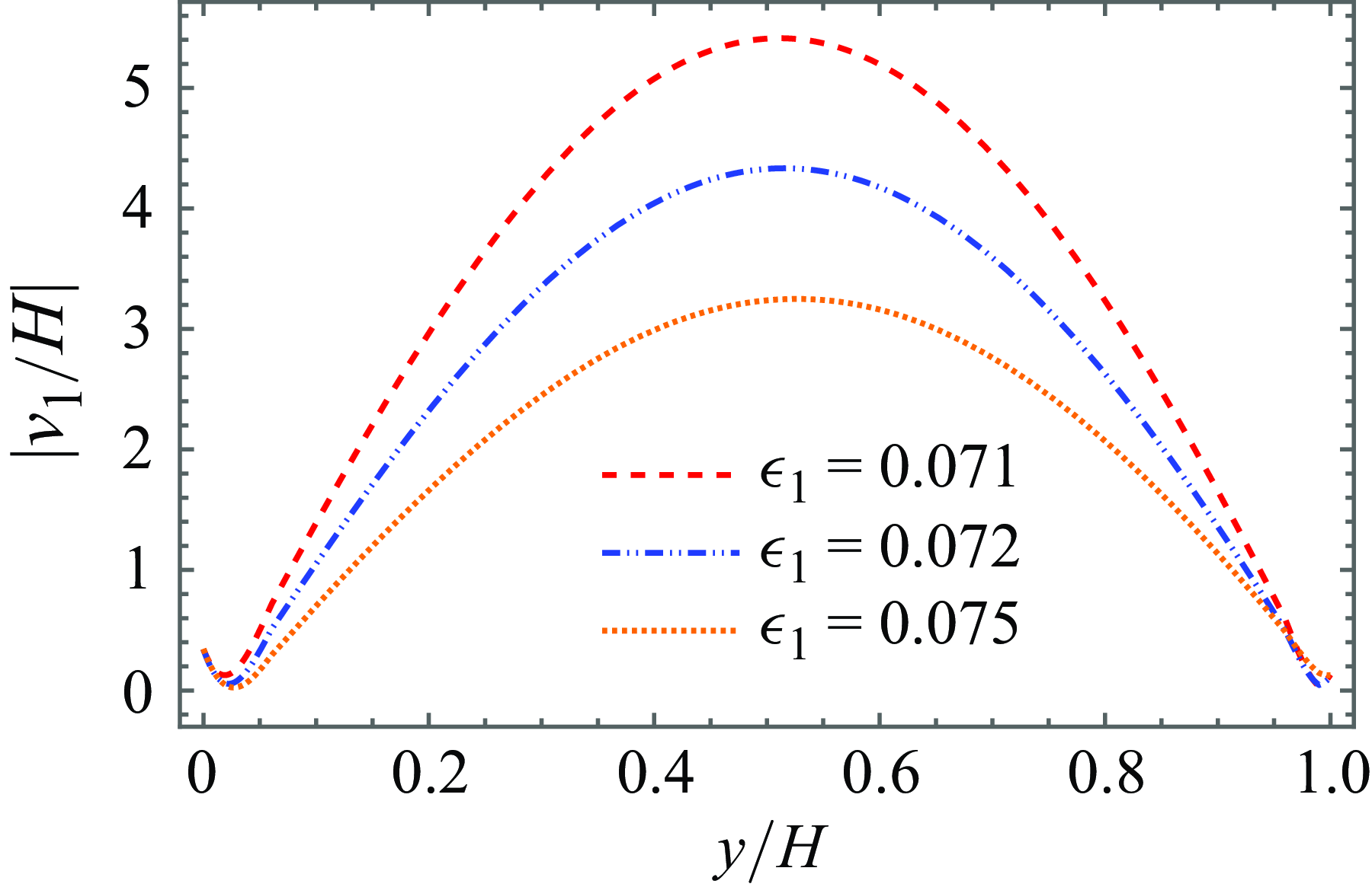
Deflection $|\nu _1/H|$ of the plate plotted against $y/H$ for different values of $\epsilon$ with $\theta =\pi /3$ , $\Gamma =1+\textrm {i}$ , $s=0.65$ , $h/H=0.6$ and $\delta =0.5$ (a) when one end is fixed and other end is free, and (b) when both ends are fixed.

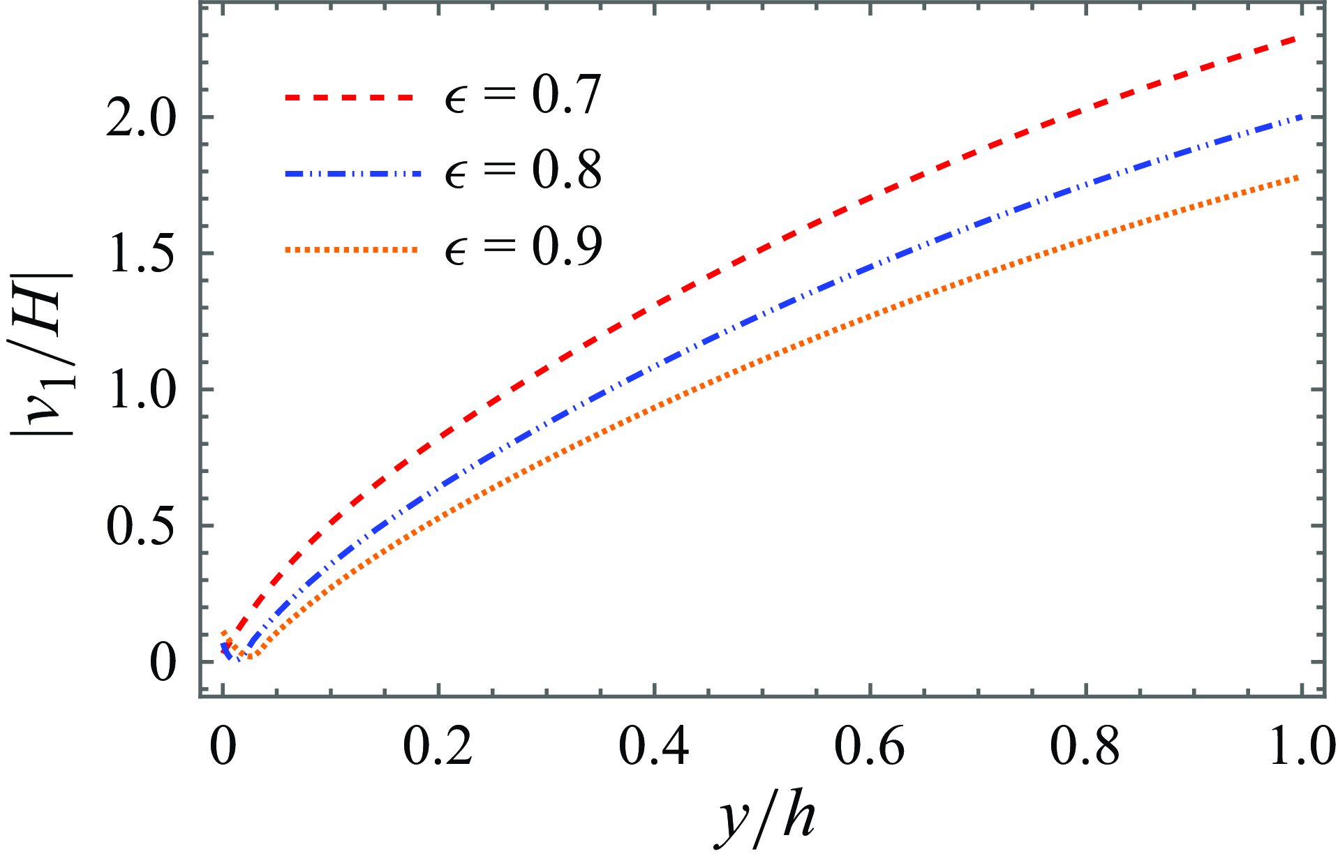
In figure 19(a), the non-dimensional deflection amplitude $|\nu _1/H|$ of the elastic porous plate is presented for different values of the flexural rigidity parameter $\epsilon$ when the plate is clamped at one end and left free at the other. In contrast, figure 19(b) shows the deflection amplitude for the case where the plate is clamped at both ends. It is observed that the plate deflection increases with a decrease in the plate flexural rigidity. This is due to the reduction in the plate flexural rigidity leads to a reduction in the stiffness of the plate against the wave motion and leads to a higher plate deflection. As shown in figure 19(b), enhanced deflection occurs near the central location of the plate, while negligible deflection is observed at the ends where it is clamped. Similar observations were found for deflection amplitude by an elastic porous plate in a single-layer fluid by Koley et al. (Reference Koley, Kaligatla and Sahoo2015).

Figure 20.

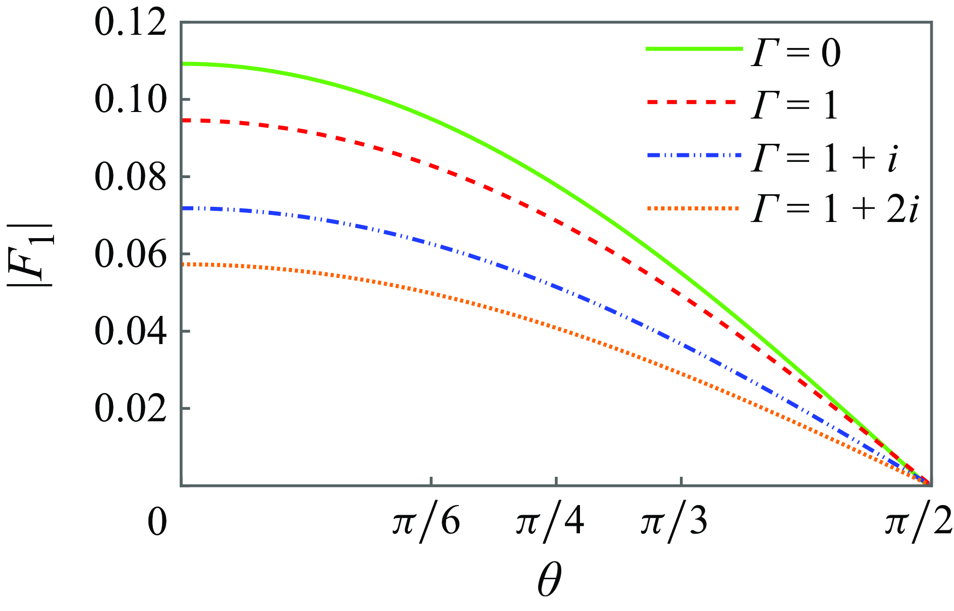
Dynamic force $|F_1|$ on the plate plotted against $\theta$ for different values of $\Gamma$ when $s=0.75$ , $h/H=0.6$ , $\epsilon =1$ and $\delta =1$ .

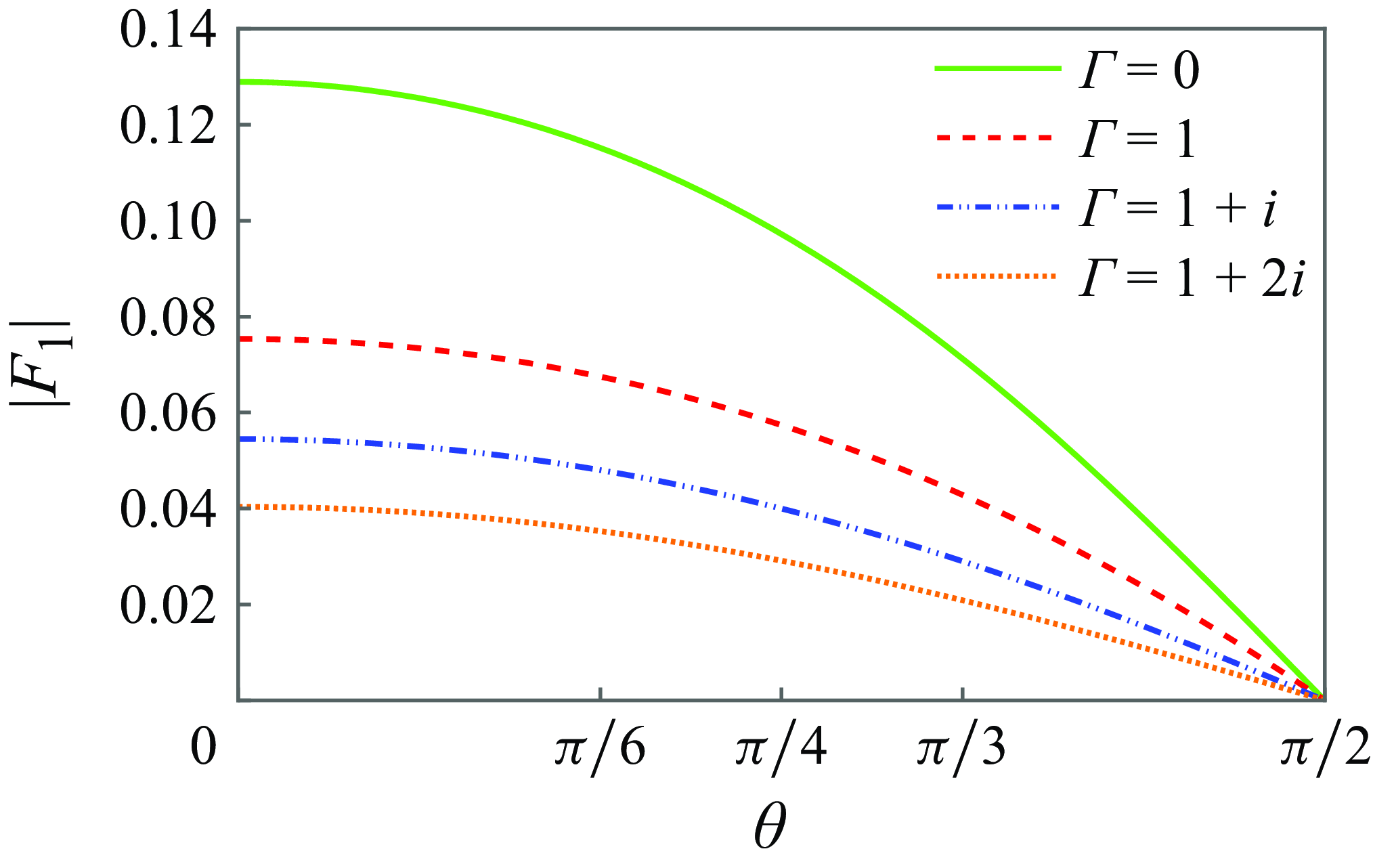
Figure 20 shows the dynamic force $|F_1|$ of the plate plotted against the angle of oblique waves $\theta$ for different values of the porous-effect parameter $\Gamma$ by fixing $s=0.75$ , $h/H=0.6$ , $\epsilon =1$ and $\delta =1$ . It is noted that the hydrodynamic force acting on the impermeable elastic plate is significantly higher than the force acting on the permeable elastic plate. The decrease in the wave force on the permeable elastic plate is due to the dissipation of wave energy by the porous structure when a wave passes through the permeable plate. Further, the hydrodynamic force is significant at a smaller oblique angle for all the porous effect parameters. Moreover, there is no hydrodynamic force at an angle closer to $90^\circ$ , and this is intuitively expected as waves pass along the plate.

5.1.2. Permeable membrane

Figure 21.

Variation of $|R_1|$ and $|T_1|$ against $m_1H$ for different values of $\Gamma$ when $\theta =\pi /3$ , $s=0.75$ , $h/H=0.5$ , $\epsilon _1=0.1$ and $\delta _1=2$ .

Figure 22.

Variation of $|R_2|$ and $|T_2|$ against $m_1H$ for different values of $\Gamma$ when $\theta =\pi /3$ , $s=0.75$ , $h/H=0.5$ , $\epsilon _1=0.1$ and $\delta _1=2$ .

Figure 23.

Variation of $|R_1|$ and $|T_1|$ against $m_1H$ for different values of $\epsilon _1$ when $\theta =\pi /3$ , $\Gamma =1+\textrm {i}$ , $s=0.75$ , $h/H=0.5$ and $\delta _1=1$ .

Reflected and transmitted wave amplitudes in SM and IM are depicted versus the wavenumber $m_1H$ while fixing $\theta =\pi /3$ , $s=0.75$ , $h/H=0.5$ , $\epsilon _1=0.1$ and $\delta _1=2$ in figures 21 and 22. Figure 21 illustrates that the reflection curves in SM increase monotonically from lower to a specific wavenumber, after which they reach a uniform value for moderate and higher wavenumbers. Figure 22 demonstrates that the reflection curves in IM rise from zero to a specific value before stabilising at a constant level. The opposite trend is noted for transmission curves in SM and IM. Figures 21 and 22 also reveal that the reflection curves in SM and IM decrease as the inertial and resistance effects of the porous parameters increase. A reverse pattern is observed in the case of wave transmission. This observation is intuitively expected, as an increase in porosity not only facilitates higher wave transmission but also reduces the membrane’s resistance to wave motion. Breakwater without porosity exhibits higher wave reflection and lower wave transmission. The present results agree well with those of Suresh Kumar et al. (Reference Suresh Kumar, Manam and Sahoo2007)

Figure 24.

Variation of $|R_2|$ and $|T_2|$ against $m_1H$ for different values of $\epsilon _1$ when $\theta =\pi /3$ , $\Gamma =1+\textrm {i}$ , $s=0.75$ , $h/H=0.5$ and $\delta _1=1$ .

In figures 23 and 24, reflection and transmission curves are depicted versus the wavenumber $m_1H$ for different values of the membrane tension parameter $\epsilon _1$ when $\theta =\pi /3$ , $\Gamma =1+\textrm {i}$ , $s=0.75$ , $h/H=0.5$ and $\delta _1=1$ are fixed. Figures 23 and 24 demonstrate that the reflection curves increase monotonically for lower wavenumbers, and they attain uniform values for moderate and higher wavenumbers. These plots also illustrate that as the membrane tension parameter increases, the reflected wave amplitude curve increases for fixed smaller wavenumbers. Then, as the wavenumber increases, the reverse pattern is noted. Opposite trends are observed for transmitted wave amplitude curves in SM and IM. It is also significantly noted that a barrier with lower stiffness produces lower wave reflection and higher wave transmission.

Reflected and transmitted wave amplitudes are plotted, in figures 25 and 26, versus the wavenumber $m_1H$ for different values of the fluid depth ratio parameter $h/H$ in SM and IM when $\theta =\pi /3$ , $\Gamma =1$ , $s=0.75$ , $\epsilon _1=0.01$ and $\delta _1=2$ are fixed. It is noted that wave reflection is higher when both layers have almost equal depth, i.e. $h/H=0.9$ . Also, the wave reflection is lower for the thinner upper layer, i.e. $h/H=0.1$ , almost over the entire range of interest. This phenomenon arises due to the resonant interaction between surface and internal waves when the free surface is close to the interface.

Figure 25.

Variation of $|R_1|$ and $|T_1|$ against $m_1H$ for different values of $h/H$ when $\theta =\pi /3$ , $\Gamma =1$ , $s=0.75$ , $\epsilon _1=0.01$ and $\delta _1=2$ .

Figure 26.

Variation of $|R_2|$ and $|T_2|$ against $m_1H$ for different values of $h/H$ when $\theta =\pi /3$ , $\Gamma =1$ , $s=0.75$ , $\epsilon _1=0.01$ and $\delta _1=2$ .

Figure 27.

Variation of $|R_1|$ and $|T_1|$ against $m_1H$ for different values of $\theta$ when $\Gamma =1+\textrm {i}$ , $s=0.75$ , $h/H=0.5$ , $\epsilon _1=0.01$ and $\delta _1=2$ .

Figure 28.

Variation of $|R_2|$ and $|T_2|$ against $m_1H$ for different values of $\theta$ when $\Gamma =1+\textrm {i}$ , $s=0.75$ , $h/H=0.5$ , $\epsilon _1=0.01$ and $\delta _1=2$ .

In figures 27 and 28, reflection and transmission coefficients are depicted in SM and IM versus the dimensionless wavenumber $m_1 H$ for various values of angle of incidence $\theta$ while fixing $\Gamma =1+\textrm {i}$ , $h/H=0.5$ , $s=0.75$ , $\epsilon _1=0.01$ and $\delta _1=2$ . It is observed that from figures 27 and 28, reflected wave amplitude curves in SM and IM increase for fixed smaller wavenumbers, and thereafter they attain a uniform value for the rest of the wavenumbers. Plots also reveal that reflected wave amplitude curves increase with a decrease in oblique angles. Moreover, it is observed that the reflected wave amplitude curves in SM and IM for $\theta =0^{\circ }$ are substantially higher compared with the other amplitude curves. This outcome is intuitively expected as waves hit the permeable membrane without making oblique angles.

Figure 29.

Deflection $|\nu _1/H|$ of the plate plotted against $y/H$ for different values of $\epsilon _1$ with $\theta =\pi /3$ , $\Gamma =1+\textrm {i}$ , $s=0.45$ , $h/H=0.45$ and $\delta _1=1$ when both ends are clamped.

In figure 29, non-dimensional deflection amplitude $|\nu _1/H|$ of the permeable membrane is plotted for different values of the membrane tension parameter $\epsilon _1$ when the membrane barrier is clamped at both ends and while fixing $s=0.45$ , $\theta =\pi /3$ , $\Gamma =1$ , $h/H=0.45$ and $\delta _1=1$ . The membrane deflection is found to increase with the decrease in membrane tension. This is attributable to the reduction in membrane tension, which decreases the stiffness of the membrane barrier against wave motion, resulting in greater deflection of the membrane. Enhanced deflection occurs near the central location of the membrane barrier and the membrane deflection is negligible at the ends where it is clamped. Similar results were reported by Suresh Kumar et al. (Reference Suresh Kumar, Manam and Sahoo2007)