1. Introduction
Non-spherical particles immersed in complex flows exhibit intricate rotation behaviours due to their shape, which are commonly observed in various natural and industrial processes. For instance, the shape of particular objects affects the collision and aggregation process of ice crystals (Pfitzenmaier et al. Reference Pfitzenmaier, Unal, Dufournet and Russchenberg2018), the transport of disk-like blood cells in vessels (Cordasco & Bagchi Reference Cordasco and Bagchi2016), the behavioural strategies of microorganisms (Lovecchio et al. Reference Lovecchio, Climent, Stocker and Durham2019; Qiu et al. Reference Qiu, Cui, Climent and Zhao2022), the dispersion of pollen (Sabban & van Hout Reference Sabban and van Hout2011) and the fibre orientation in paper fabrication (Lundell, Söderberg & Alfredsson Reference Lundell, Söderberg and Alfredsson2011). Compared with spheres, non-spherical particles possess additional orientational degrees of freedom. In many natural and industrial flow scenarios, such particles can be reasonably approximated as ellipsoids due to their smooth shapes and geometric simplicity. A commonly used subclass is the spheroidal ellipsoid, which exhibits axisymmetry. For a spheroid, the shape is characterized by the aspect ratio
 $\lambda = a/b$
, where
 $a$
and
 $b$
denote the semilengths of the symmetry axis and the equatorial axis, respectively. The rotational dynamics of such particles are strongly influenced by both the vorticity and the strain-rate components of the local velocity gradient tensor, resulting in dynamics that are considerably more complex than those of spherical particles. These effects are further modulated by the particle aspect ratio, leading to diverse behaviours. Meanwhile, in many practical situations, such as sediment grains, industrial powder particles or heavy biological matter, the particle density far exceeds that of the surrounding fluid. The rotational dynamics of these large-density particles, often referred to as inertial spheroids, are significantly affected by fluid–particle slip. Their rotations are governed not only by the local strain and vorticity of the carrier flow but also by the fluid-inertial torque induced by the slip velocity, which becomes more pronounced at large-density ratios. For instance, the strong velocity gradients in wall-bounded shear flows will allow particles with large density-ratio to experience both significant shear and considerable slip relative to the fluid (Cui et al. Reference Cui, Qiu, Jiang and Zhao2023, Reference Cui, Liu, Qiu and Zhao2024). The combined effects of anisotropic particle shape, finite density ratio and fluid–particle slip result in complicated rotational dynamics. Understanding these effects is thus of both fundamental and practical interest. In this study, we consider a large density-ratio spheroid immersed in a simple shear flow with a streamwise fluid–particle slip velocity as a prototype model to explore these effects systematically.
1.1. Angular dynamics of spheroidal particles in shear flows
The rotational dynamics of non-spherical particles immersed in a linear shear flow were first investigated by Jeffery (Reference Jeffery1922), who derived the viscous torque acting on ellipsoidal particles in a creeping shear flow. When the fluid inertia and particle inertia are weak enough to ignore the inertial effect, the particle is torque-free. For spheroidal particles, this leads to a family of closed periodic orbits traced by the particle symmetry axis, named Jeffery orbits (Jeffery Reference Jeffery1922). After that, Taylor (Reference Taylor1923) experimented with non-spherical particles within a shear flow formed by a concentric rotating cylinders, demonstrating the validity of the Jeffery torque model as well as the minimum dissipation hypothesis when considering a weak inertial effect (Jeffery Reference Jeffery1922). Regarding a triaxial inertialess ellipsoid, Hinch & Leal (Reference Hinch and Leal1979) found doubly periodic motion, and Yarin, Gottlieb & Roisman (Reference Yarin, Gottlieb and Roisman1997) found the range of shape parameter that allows inertialess ellipsoidal particles to rotate chaotically in the linear shear flow via theoretical analysis, especially for the particle shape close to prolate spheroids. Besides, Einarsson et al. (Reference Einarsson, Mihiretie, Laas, Ankardal, Angilella, Hanstorp and Mehlig2016) conducted an experiment of asymmetric rods in a microchannel, and the experimental results demonstrates that the tumbling of rods in shear flows may be periodic, doubly periodic or possibly chaotic, relying on the particle shape. These results are consistent with the theory (Hinch & Leal Reference Hinch and Leal1979; Yarin et al. Reference Yarin, Gottlieb and Roisman1997).
The presence of particle inertia changes the rotational dynamics of the spheroid, which can be solved by the Euler equations in a particle-fixed coordinate under the influence of external torques (Lundell & Carlsson Reference Lundell and Carlsson2010; Lundell Reference Lundell2011; Challabotla, Nilsen & Andersson Reference Challabotla, Nilsen and Andersson2015). When the shear Reynolds number of particles, defined as
 ${\textit{Re}}_\kappa =\kappa l^2/\nu$
, remains much smaller than one, the dominant torque acting on the spheroid arises from viscous stress, leading to the classical Jeffery torque (Jeffery Reference Jeffery1922). Here,
 $l$
denotes the semilength of the spheroid’s major axis,
 $\kappa$
is the shear rate and
 $\nu$
is the kinematic viscosity of the fluid. The particle inertia can be estimated by the rotational Stokes number, defined as
 $St_r=D_{{\kern-1pt}pf}\kappa l/\nu$
, where
 $D_{{\kern-1pt}pf}$
is the particle–fluid density ratio. Interestingly,
 $St_r\equiv D_{{\kern-1pt}pf} {\textit{Re}}_\kappa$
. As particle inertia increases, in the linear shear flow, prolate spheroids tend to tumble with their symmetry axes rotating in the flow-gradient plane (Lundell & Carlsson Reference Lundell and Carlsson2010), while oblate spheroids tend to logroll with their symmetry axes aligned to the vortical axis (Challabotla et al. Reference Challabotla, Nilsen and Andersson2015). Moreover, the trajectories of the endpoints of symmetry axes are different with various particle inertia and shapes (Lundell & Carlsson Reference Lundell and Carlsson2010; Challabotla et al. Reference Challabotla, Nilsen and Andersson2015). When particle inertia is very large or small, the spheroids will spend more time approaching the equilibrium rotation (Lundell & Carlsson Reference Lundell and Carlsson2010; Challabotla et al. Reference Challabotla, Nilsen and Andersson2015). For triaxial ellipsoids, the presence of particle inertia stabilizes the rotations of ellipsoids to the mode of rotation about the shortest principal axis aligned with the ambient vortical axis (Lundell Reference Lundell2011). When particle inertia exceeds a critical threshold, this rotation mode becomes dominant regardless of the specific ellipsoidal shape (Lundell Reference Lundell2011). The mechanisms of these phenomena have been elucidated by using Floquet stability analysis (Lundell Reference Lundell2011; Einarsson, Angilella & Mehlig Reference Einarsson, Angilella and Mehlig2014; Cui et al. Reference Cui, Zhao, Huang and Xu2019). In addition, if the shear flow is oscillating, the quasi-two-dimensional rotation of spheroids within the flow-gradient plane exhibits chaotic signatures depending on the frequency of oscillation and particle inertia (Nilsen & Andersson Reference Nilsen and Andersson2013; Jiang et al. Reference Jiang, Huang, Xu and Zhao2022).
When
 ${\textit{Re}}_\kappa$
is not much smaller than one, the shear-induced fluid inertia can significantly influence the rotational dynamics of spheroidal particles. Earlier studies (Qi & Luo Reference Qi and Luo2002, Reference Qi and Luo2003; Yu, Phan-Thien & Tanner Reference Yu, Phan-Thien and Tanner2007; Huang et al. Reference Huang, Yang, Krafczyk and Lu2012; Rosén et al. Reference Rosén, Lundell and Aidun2014, Reference Rosén, Do-Quang, Aidun and Lundell2015, Reference Rosén, Nordmark, Aidun, Do-Quang and Lundell2016, Reference Rosén, Kotsubo, Aidun, Do-Quang and Lundell2017; Rosén Reference Rosén2017) numerically investigated the complicated rotations of neutrally buoyant and finite-size ellipsoids in simple shear flows, accounting for both particle inertia and fluid inertia. In those studies, the fluid-inertial effect arises from the shear and added mass, whereas the one due to the slip velocity between particle and fluid is absent. The rotation modes of spheroids vary with
 ${\textit{Re}}_\kappa$
and particle shapes. For prolate spheroids, with the shear Reynolds number
 ${\textit{Re}}_\kappa$
increasing, the rotation modes of prolate spheroids experience Jeffery orbit, tumbling, tumbling–logrolling (TL), tumbling–inclined–rolling, tumbling–inclined–kayaking, kayaking and steady aligning state (Huang et al. Reference Huang, Yang, Krafczyk and Lu2012; Rosén et al. Reference Rosén, Lundell and Aidun2014). Similarly, regarding oblate spheroids, the final rotation modes experience Jeffery orbit, logrolling, tumbling–inclined–rolling and steady aligning state as shear Reynolds number
 ${\textit{Re}}_\kappa$
increases (Huang et al. Reference Huang, Yang, Krafczyk and Lu2012). These complicated motions observed in particle-resolved (PR) simulations result from the competition between fluid inertia and particle inertia in the shear flows. Moreover, Rosén (Reference Rosén2017) discovered that the logrolling mode of prolate spheroids with a large aspect ratio exhibits Shilnikov bifurcation or chaos because of the existence of fluid inertia and particle inertia. For triaxial ellipsoids that rotate chaotically at low shear Reynolds numbers (Hinch & Leal Reference Hinch and Leal1979; Yarin et al. Reference Yarin, Gottlieb and Roisman1997; Lundell Reference Lundell2011; Cui et al. Reference Cui, Zhao, Huang and Xu2019), the rotation about the middle principal axis of the ellipsoid is stabilized by the fluid inertia with shear Reynolds number growing up (Rosén et al. Reference Rosén, Kotsubo, Aidun, Do-Quang and Lundell2017). Furthermore, Einarsson et al. (Reference Einarsson, Candelier, Lundell, Angilella and Mehlig2015), Meibohm et al. (Reference Meibohm, Candelier, Rosén, Einarsson, Lundell and Mehlig2016) and Dabade, Marath & Subramanian (Reference Dabade, Marath and Subramanian2016) theoretically investigated the influence of the weak fluid inertia on the rotation of spheroidal particles within simple shear flows at small shear Reynolds numbers by using perturbation theory and the reciprocal theorem. They found that the fluid-inertial torque at regular order
 $O({\textit{Re}}_\kappa )$
drives drifts of symmetry axis while the singular fluid-inertial torque at
 $O({\textit{Re}}_\kappa ^{3/2})$
affects the time period within an orbit (Dabade et al. Reference Dabade, Marath and Subramanian2016; Marath & Subramanian Reference Marath and Subramanian2017). Recently, Giusto et al. (Reference Giusto, Bergougnoux, Marchioli and Guazzelli2024) found that in experiments prolate spheroids are uniquely driven towards a tumbling motion while oblate spheroids have two equilibrium rotations (tumbling and logrolling), depending on the initial orientation. These findings are qualitatively consistent with the theories derived by Einarsson et al. (Reference Einarsson, Candelier, Lundell, Angilella and Mehlig2015), Meibohm et al. (Reference Meibohm, Candelier, Rosén, Einarsson, Lundell and Mehlig2016) and Dabade et al. (Reference Dabade, Marath and Subramanian2016), though these theories overestimate the fluid-inertial effect.
Most earlier studies in shear flows neglect slip velocity at the centre of the spheroid. However, recent research discovered the non-trivial influence of the slip-induced fluid-inertial torque in the settling problem (Gustavsson et al. Reference Gustavsson, Sheikh, Lopez, Naso, Pumir and Mehlig2019; Anand, Ray & Subramanian Reference Anand, Ray and Subramanian2020; Sheikh et al. Reference Sheikh, Gustavsson, Lopez, Lévêque, Mehlig, Pumir and Naso2020), where the gravity induces a pronounced slip velocity. Moreover, Bhowmick et al. (Reference Bhowmick, Seesing, Gustavsson, Guettler, Wang, Pumir, Mehlig and Bagheri2024) observed strong orientation fluctuations of non-spherical particles settling in the atmosphere in experiments, which has been theoretically illustrated by considering this fluid-inertial torque model (Dabade, Marath & Subramanian Reference Dabade, Marath and Subramanian2015). Although these findings can be primarily attributed to the analytical fluid-inertial torque model at low particle Reynolds numbers derived by Dabade et al. (Reference Dabade, Marath and Subramanian2015), there still remains a gap in understanding the impact of this fluid-inertial torque on particle behaviours in flows that incorporate both shear and slip velocities. To the best of the authors’ knowledge, Li et al. (Reference Li, Cui, Huang, Zhao and Xu2018) was the first to delve into such inquiries in a bounded shear flow via the immersed boundary method. In their work, the slip velocity exists along the streamwise direction. Their investigation revealed a departure from the continuous rotation in the flow-gradient plane as the particle Reynolds number
 ${\textit{Re}}_{\!p}$
increases (Li et al. Reference Li, Cui, Huang, Zhao and Xu2018). Then, spheroidal particles tend to reach a steady state where their symmetry axes are inclined to the streamwise direction because of the combined effect of shear and fluid-inertial torques (Li et al. Reference Li, Cui, Huang, Zhao and Xu2018). Regarding low Reynolds number, Cui et al. (Reference Cui, Qiu, Jiang and Zhao2023) discovered similar results between point-particle (PP) and PR simulations employing the immersed boundary method. Recently, Cui et al. (Reference Cui, Liu, Qiu and Zhao2024) investigated the angular dynamics of spheroids in shear flows with a streamwise slip velocity at the centre point via PP simulations, and found prolate spheroids tend to logroll while oblate spheroids tend to tumble or align with a steady orientation when the slip-induced fluid-inertial torque dominates, which is opposite to the earlier results in the absence of fluid-inertial torque. At the same time, when the effects of fluid-inertial torque and particle inertia are comparable, prolate and oblate spheroids both exhibit two equilibrium rotation modes, i.e. tumbling and logrolling, depending on the initial orientations (Cui et al. Reference Cui, Liu, Qiu and Zhao2024). Moreover, in addition to the TL mode, oblate spheroids also have other multistable rotation modes, i.e. aligning–tumbling (AT), aligning–tumbling–logrolling (ATL) rotation modes, depending upon initial orientations (Cui et al. Reference Cui, Liu, Qiu and Zhao2024). These reflect a non-trivial influence of fluid-inertial torque on the rotational dynamics of inertial spheroidal particles. Note that the shear-flow configurations in both Li et al. (Reference Li, Cui, Huang, Zhao and Xu2018) and Cui et al. (Reference Cui, Liu, Qiu and Zhao2024) correspond to vertical shear with gravity aligned with the streamwise direction. In these studies, however, particle translation was constrained, yielding a constant slip velocity, whereas in a realistic vertical shear flow the slip velocity varies dynamically during the settling of the spheroid. Nevertheless, the various rotation modes reported in Cui et al. (Reference Cui, Liu, Qiu and Zhao2024) were obtained by traversing a wide range of particle parameters, and lacked a general framework for predicting stable rotation modes as functions of these parameters. This motivates the present investigation.
1.2. Linear stability analysis on the angular dynamics of non-spherical particles
Linear stability analysis is a powerful tool to determine the stability of different equilibrium rotational modes of particles. Depending on the nature of the equilibrium state, two main types of linear stability analysis are commonly employed: one for fixed points and the other for periodic motions. The latter is commonly referred to as Floquet theory. In previous studies, stability analysis of particle rotation has primarily focused on triaxial ellipsoidal particles in simple shear flows. In such cases, the equilibrium rotation mode about each particle axis is periodic, making fixed-point linear stability analysis inapplicable. Floquet theory is used by Yarin et al. (Reference Yarin, Gottlieb and Roisman1997) to identify ranges of shape parameters in which inertia-free elongated triaxial ellipsoids exhibit unstable rotational dynamics about their three principal axes in shear flows. Building upon this framework, Lundell (Reference Lundell2011) revealed that particle inertia can significantly stabilize rotational dynamics. Rosén et al. (Reference Rosén, Kotsubo, Aidun, Do-Quang and Lundell2017) further investigated the stability of finite-size triaxial ellipsoids via direct numerical simulations. For spheroidal particles with weak particle inertia, Einarsson et al. (Reference Einarsson, Angilella and Mehlig2014) derived analytical expressions for the Floquet exponent through a small parameter expansion. Extending this work, Cui et al. (Reference Cui, Zhao, Huang and Xu2019) numerically examined the rotational stability of both spheroidal and triaxial ellipsoidal particles across a wide range of particle inertia, revealing a narrow interval of parameters wherein stable rotation around the intermediate axis is possible. As the influence of slip-induced fluid-inertial torque on particles in shear flow has attracted increasing attention, it becomes particularly interesting to apply linear stability theory to examine various rotation modes of spheroids as functions of slip velocity, aspect ratio and particle inertia. The advantage of this approach lies in its focus on equilibrium states, independent of initial conditions. Consequently, this method can efficiently predict the final rotation stability at a low computational cost, avoiding the need to traverse all initial conditions.
The remainder of this paper is organized as follows. In § 2, we introduce the models of angular dynamics of spheroidal particles, and the slip-induced fluid-inertial torque. In § 3, we introduce different stability analysis methods on inertial spheroids for different Stokes numbers. In § 4, we compare the results between the stability analysis and numerical simulations. Finally, we draw conclusions in § 5.
2. Model
2.1. Physical model of a spheroid rotating in a linear shear flow
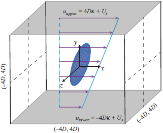
In this study, the flow we considered is formulated by
 $u=\kappa y+ U_s$
, which is a synthesis of a linear shear flow (
 $u_\kappa =\kappa y$
) and a uniform flow (
 $U_s$
), as depicted in figure 1. Here,
 $\kappa$
is the shear rate and
 $u$
is the streamwise velocity. Moreover, the corresponding velocity gradient is
 $\unicode{x1D63C}^*$
, where the components are zero except for
 $A_{xy}^*=\kappa$
. Hence, the strain-rate tensor
 $\unicode{x1D64E}^{\;*}$
and the rotation tensor
 $\unicode{x1D64A}^*$
are expressed as follows:
 \begin{equation} \unicode{x1D64E}^{\;*}=\left [\begin{matrix} 0 & \kappa /2 & 0 \\ \kappa /2 & 0 & 0 \\ 0 & 0 & 0 \end{matrix}\right ]\!,\quad \unicode{x1D64A}^{\;*}=\left [\begin{matrix} 0 & \kappa /2 & 0 \\ -\kappa /2 & 0 & 0 \\ 0 & 0 & 0 \end{matrix}\right ]\!. \end{equation}
The rotation of fluid
 $\boldsymbol \varOmega ^*$
is
 $[0,0,-\kappa /2]^T$
, which is perpendicular to the flow-gradient plane, i.e.
 $x\!{-}\!y$
plane and, therefore, coincides with the
 $z$
-axis. Mostly, the
 $z$
-axis is also called the vortical axis.
Schematic of the synthesis shear flow of
 $u=\kappa y+U_s$
.

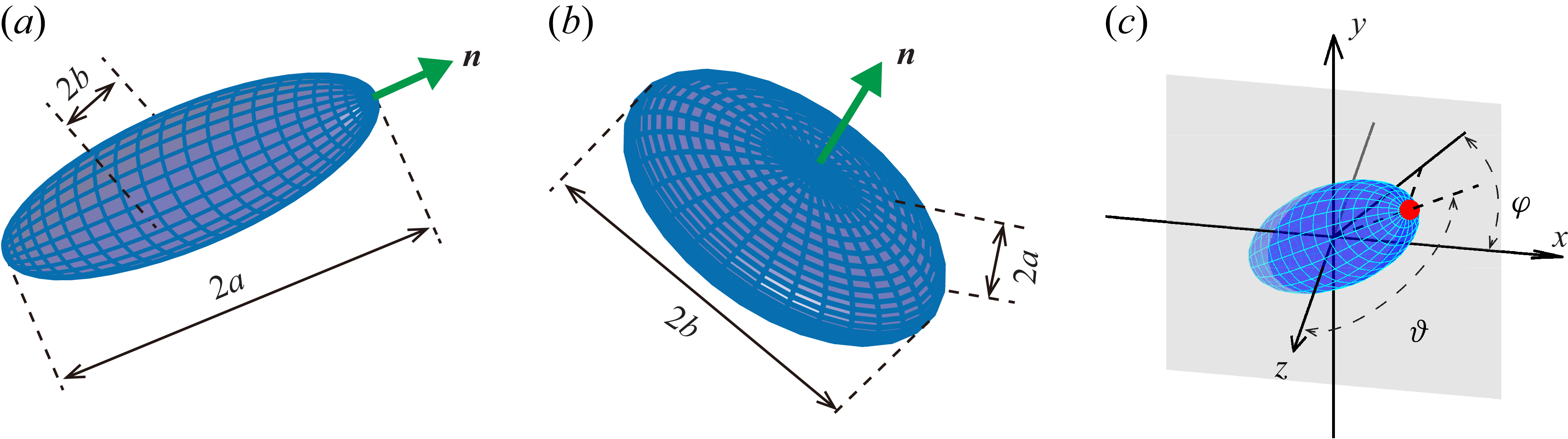
In this study, we consider spheroidal particles, which are axisymmetric, as shown in figure 2. The ratio of the symmetry axis (
 $2a$
) to the equatorial axis (
 $2b$
) is denoted as aspect ratio
 $\lambda =a/b$
. Meanwhile, we also use shape parameter
 $\varLambda =(\lambda ^2-1)/(\lambda ^2+1)$
to regularize shape within
 $(-1,1)$
. Therefore, prolate spheroids have
 $\lambda \gt 1(0\lt \varLambda \lt 1)$
, while oblate spheroids have
 $0\lt \lambda \lt 1(-1\lt \varLambda \lt 0)$
. For the spherical one, the aspect ratio is
 $\lambda =1$
and the corresponding shape parameter
 $\varLambda$
is equal to zero. The orientation of a spheroid is defined by the direction of its symmetry axis, denoted by the unit vector
 $\boldsymbol{n}$
. Two Euler angles,
 $\varphi$
and
 $\vartheta$
, are introduced as shown in figure 2(c). The azimuthal angle
 $\varphi$
measures the angle between the
 $x$
-axis and the projection of
 $\boldsymbol{n}$
onto the
 $x$
–
 $y$
plane, while the polar angle
 $\vartheta$
denotes the angle between
 $\boldsymbol{n}$
and the vorticity (or
 $z$
) axis. In this study, the centre of a spheroidal particle is set at
 $y=0$
, where a slip velocity between particle and fluid exists, denoted as
 $u_s\equiv U_s$
. This configuration is consistent with earlier studies (Li et al. Reference Li, Cui, Huang, Zhao and Xu2018; Cui et al. Reference Cui, Liu, Qiu and Zhao2024), which is similar to a spheroid settling in a vertical shear flow with a gravity along to the flow. Nevertheless, the slip velocity is constant in the present study.
Schematic of (a) prolate and (b) oblate spheroids, where green arrows represent the direction of the symmetry axes. (c) Euler angles (
 $\varphi$
,
 $\vartheta$
) of symmetry axis.
In the current study, there are two Reynolds numbers. One is the particle Reynolds number based on the slip velocity, namely
 ${\textit{Re}}_{\!p}=u_sl/\nu$
, where
 $l$
is the semilength of the major axis and
 $\nu$
is the fluid kinematic viscosity. The other one is the shear Reynolds number defined as
 ${\textit{Re}}_\kappa =\kappa l^2/\nu$
, reflecting the effect of fluid inertia from shear. Throughout this study, we primarily consider cases with
 ${\textit{Re}}_{\!p}, {\textit{Re}}_\kappa \lt 1$
to minimize the influence of high-order fluid inertia. The non-dimensional parameters that correspond to particle inertia are the rotational and translational Stokes numbers. Here, only the rotational Stokes number, denoted as
 $St_r$
, should be taken into account, because the translational motions are constrained in this study. Note that rotational Stokes number is defined as
 $St_r=D_{{\kern-1pt}pf}\kappa l^2/\nu \equiv D_{{\kern-1pt}pf} {\textit{Re}}_\kappa$
, where
 $D_{{\kern-1pt}pf}$
is the density ratio between particle and fluid. For the sake of simplicity, hereinafter, the Stokes number only represents the rotational Stokes number. In addition, we focus on large density ratios (
 $D_{{\kern-1pt}pf} \gg 1$
), such that the fluid inertia associated with the added mass can be neglected.
2.2. Angular dynamics of spheroids
According to Lundell & Carlsson (Reference Lundell and Carlsson2010) and Challabotla et al. (Reference Challabotla, Nilsen and Andersson2015), the angular dynamics of spheroids are computed in the particle coordinate by the following equation:
 \begin{equation} \unicode{x1D644}^{\,\prime } \frac {\mathrm{d}{{\boldsymbol{\omega}^*}^{\prime }}}{\mathrm{d}t^*}+{\boldsymbol{\omega}^*}^{\prime }\times \unicode{x1D644}^{\;\prime }\boldsymbol{\cdot }{\boldsymbol{\omega}^*}^{\prime } = {\boldsymbol{T}}^{\prime }. \end{equation}
Here,
 $\unicode{x1D644}^{\;\prime}$
is the moment of inertia,
 ${\boldsymbol{\omega}^*}^{\prime }$
is the rotation of particle and
 $\boldsymbol{T'}$
is the resultant torque acting on spheroid. Note that
 $(\boldsymbol{\cdot })'$
denotes variables expressed in the particle coordinate, where the vectors (or tensors) are defined with respect to the laboratory reference frame but their components are written in a Cartesian basis attached to the particle. The left-hand side of (2.2) represents the dynamics of the rigid body, referring to the particle inertia. For a spheroidal particle, the moment of inertia is expressed as
 \begin{equation} \unicode{x1D644}^{\;\prime}=\frac {1}{5}m_{\!p}\left [\begin{matrix} 2b^2&0&0\\ 0&a^2+b^2&0\\ 0&0&a^2+b^2 \end{matrix}\right ]\!, \end{equation}
where
 $m_{\!p}$
is the mass of spheroidal particle, i.e.
 $m_{\!p}=({4}/{3})\rho _{\!p}\pi a b^2$
. Here,
 $\rho _{\!p}$
is the density of the particle. To describe quantities in different frames, a vector
 $\boldsymbol{p}$
in the laboratory reference frame can be transformed from the particle coordinate by
 $\boldsymbol{p} = \unicode{x1D64D} \boldsymbol{\cdot }\boldsymbol{p'}$
, while a matrix
 $\unicode{x1D63D}$
in the laboratory reference frame can be transformed from the particle coordinate via
 $\unicode{x1D63D}=\unicode{x1D64D} \boldsymbol{\cdot }\unicode{x1D63D}' \boldsymbol{\cdot }\unicode{x1D64D}^T$
. Here,
 $\unicode{x1D64D}$
is a rotation matrix, which is defined as follows:
 \begin{equation} \unicode{x1D64D}=\left [\begin{matrix} e_0^2+e_1^2-e_2^2-e_3^2 & 2(e_1e_2-e_0e_3) & 2(e_1e_3+e_0e_2) \\ 2(e_1e_2+e_0e_3) & e_0^2-e_1^2+e_2^2-e_3^2 & 2(e_2e_3-e_0e_1) \\ 2(e_1e_3-e_0e_2) & 2(e_2e_3+e_0e_1) & e_0^2-e_1^2-e_2^2+e_3^2 \end{matrix}\right ]\!, \end{equation}
where
 $\boldsymbol e=[e_0,e_1, e_2, e_3]$
are unit quaternions. The corresponding evolution of
 $\boldsymbol{e}$
can be expressed by
 \begin{equation} \frac {\mathrm{d}{\boldsymbol{e}}}{\mathrm{d}t^*}=\unicode{x1D642}^T\boldsymbol{\cdot }\boldsymbol{\omega}^{* \prime }. \end{equation}
Here,
 \begin{equation} \unicode{x1D642}=\left [\begin{matrix} -e_1 & e_0 & -e_3 & e_2 \\ -e_2 & -e_3 & e_0 & e_1 \\ -e_3 & e_2 & -e_1 & e_0 \end{matrix}\right ]\!. \end{equation}
In this study, the resultant torque
 $\boldsymbol{T'}$
consists of Jeffery torque
 $T_{\!J}$
and fluid-inertial torque
 $T_I$
. The Jeffery torque in any frame satisfies the following form (Brenner Reference Brenner1963):
 \begin{equation} \boldsymbol T_{\!J}=\unicode{x1D646}_R\boldsymbol{\cdot }(\boldsymbol \varOmega ^*-\boldsymbol \omega ^*)+\unicode{x1D643} : \unicode{x1D64E}^{\;*}, \end{equation}
where
 $\unicode{x1D646}_R$
and
 $\unicode{x1D643}$
are the resistant coefficient tensors of rotation and shear, respectively, only related to the particle shape and the viscosity of the fluid. Note that
 $\unicode{x1D643}$
is a third-order tensor. In the particle coordinate,
 \begin{align} T^{\prime}_{J x} &=\frac {16\pi \mu b^3}{3\chi _\perp }\big(\varOmega ^{*\prime }_x-\omega ^{*\prime }_x\big),\nonumber\\ T^{\prime}_{J y} &=\frac {16\pi \mu b^3}{3(\lambda ^2\chi _\parallel +\chi _\perp )}\big[(1-\lambda ^2)S^{*\prime }_{xz}+(1+\lambda ^2)\big(\varOmega ^{*\prime }_y-\omega ^{*\prime }_y\big)\big],\nonumber\\T^{\prime}_{J z} &=\frac {16\pi \mu b^3}{3(\lambda ^2\chi _\parallel +\chi _\perp )}\big[(\lambda ^2-1)S^{*\prime }_{xy}+(\lambda ^2+1)\big(\varOmega ^{*\prime }_z-\omega ^{*\prime }_z\big)\big]. \end{align}
Here,
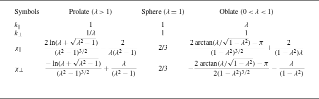
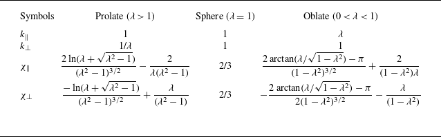
 $\chi _\perp$
and
 $\chi _\parallel$
are the integral shape parameters as listed in table 1. Note that the subscript
 $\parallel$
means the coefficients along the symmetry axis while the subscript
 $\perp$
represents the coefficients normal to the symmetry axis. The fluid-inertial torque in the Eulerian frame is expressed as
 \begin{equation} \boldsymbol T_I =-\rho _{\!f}r_{\!p}^3 F_\lambda (\boldsymbol u_s \boldsymbol{\cdot }\boldsymbol{n})(\boldsymbol u_s\times \boldsymbol n), \end{equation}
where
 $r_{\!p}$
represents the semilength of the major axis of the spheroid, i.e.
 $r_{\!p}=a$
for probate spheroids and
 $r_{\!p}=b$
for oblate spheroids. In the particle coordinate,
 \begin{equation} \boldsymbol T^{\prime}_I =-\rho _{\!f}r_{\!p}^3 F_\lambda u^{\prime}_{s 1}\left (\begin{matrix} 0\\ u^{\prime}_{s 3} \\[3pt] -u^{\prime}_{s 2} \end{matrix}\right )\!, \end{equation}
where
 $u^{\prime}_{s 1}$
,
 $u^{\prime}_{s 2}$
and
 $u^{\prime}_{s 3}$
are the three components of slip velocity in the particle coordinate, respectively. Note that
 $F_\lambda$
is a function of fluid-inertial torque depending on particle shape (Dabade et al. Reference Dabade, Marath and Subramanian2015) (see Appendix A).
Shape parameters of a spheroid.
In the shear flow, we use the shear rate
 $\kappa$
to non-dimensionlize the angular dynamics of spheroids, i.e. particle rotation
 $\boldsymbol \omega =\boldsymbol \omega ^*\!/\!\kappa$
, fluid rotation
 $\boldsymbol \varOmega =\boldsymbol \varOmega ^*\!/\!\kappa$
, strain-rate
 $\unicode{x1D64E}=\unicode{x1D64E}^{\;*}\!/\!\kappa$
, fluid rotation tensor
 $\unicode{x1D64A}=\unicode{x1D64A}^*\!/\!\kappa$
and time
 $t=t^*\kappa$
. The non-dimensional governed equations of angular dynamics of inertial spheroidal particles in the Eulerian frame are expressed as follows:
 \begin{align} St_r \unicode{x1D63E}\boldsymbol{\cdot }\frac {\mathrm{d}{\boldsymbol \omega }}{\mathrm{d}t}+\boldsymbol{n}\times (St_r C_\perp \varLambda \boldsymbol \omega \boldsymbol \omega )\boldsymbol{\cdot }\boldsymbol n&=\boldsymbol \varOmega -\boldsymbol \omega +\boldsymbol n\times \varLambda \unicode{x1D64E} \boldsymbol{\cdot }\boldsymbol n+\boldsymbol n\times M\hat {\boldsymbol u}_s\hat {\boldsymbol u}_s\boldsymbol{\cdot }\boldsymbol n,\nonumber \\ \frac {\mathrm{d}{\boldsymbol n}}{\mathrm{d}t}&=\boldsymbol \omega \times \boldsymbol n. \end{align}
Here,
 $\boldsymbol n$
is the direction of the symmetry axis of the spheroid, and the left-hand side equation refers to the particle inertia term. In the right-hand side,
 $\boldsymbol \varOmega -\boldsymbol \omega +\boldsymbol n\times \varLambda \unicode{x1D64E} \boldsymbol{\cdot }\boldsymbol n$
is the term of Jeffery torque, while
 $\boldsymbol n\times M\hat {\boldsymbol u}_s\hat {\boldsymbol u}_s\boldsymbol{\cdot }\boldsymbol n$
is the term of fluid-inertial torque. Moreover,
 $\hat {\boldsymbol u}_s$
is a unit vector of slip velocity, which directs to the streamwise direction. Meanwhile,
 $\unicode{x1D63E}$
,
 $C_\perp$
and
 $\varLambda$
are coefficients related to particle shape, i.e.
 \begin{align} \unicode{x1D63E} & =C_\parallel \boldsymbol n\boldsymbol n+C_\perp (\unicode{x1D640}-\boldsymbol n \boldsymbol n), \nonumber \\ C_\perp & =\frac {k_\perp ^2k_\parallel (k_\perp ^2\chi _\perp +k_\parallel ^2\chi _\parallel )}{20}, \nonumber \\ C_\parallel & =\frac {2k_\perp ^4k_\parallel \chi _\perp }{20}, \nonumber \\ \varLambda & =\frac {k_\parallel ^2-k_\perp ^2}{k_\parallel ^2+k_\perp ^2}\equiv \frac {\lambda ^2-1}{\lambda ^2+1}. \end{align}
Here,
 $k_\perp$
,
 $k_\parallel$
are shape parameters as listed in table 1, which are defined as
 $k_\perp =b/r_{\!p}$
and
 $k_\parallel =a/r_{\!p}$
, respectively. Note that
 $r_{\!p}$
is the semilength of the major axis of spheroids, depending on whether the shape is prolate or oblate. Meanwhile,
 $M$
reflects the direction and the strength of fluid-inertial torque, which is linked to particle shape, slip velocity and shear rate, i.e.
 \begin{equation} M =\frac {3 F_\lambda \big(k_{\perp }^2\chi _\perp +k_{\parallel }^2\chi _\parallel \big) }{16\pi \big(k_{\perp }^2+k_{\parallel }^2\big)}\frac {u_s^2}{\nu \kappa }. \end{equation}
Here, the ratio
 $u_s^2/\nu \kappa$
, denoted as
 $\zeta ^2$
, reflects the relative importance of the fluid-inertial torque compared with the Jeffery torque (Sheikh et al. Reference Sheikh, Gustavsson, Lopez, Lévêque, Mehlig, Pumir and Naso2020), i.e.
 $\zeta ^2\sim |\boldsymbol T_I|/|\boldsymbol T_{\!J}|$
. A larger
 $\zeta$
indicates a stronger effect of fluid-inertial torque because
 $|M|\propto \zeta ^2$
. Moreover, the definition
 $\zeta ^2=u_s^2/\nu \kappa$
can also be reformulated as
 $\zeta ^2 ={\textit{Re}}_{\!p}^2 /{\textit{Re}}_\kappa$
, leading to
 $\zeta ={\textit{Re}}_{\!p}/\sqrt {{\textit{Re}}_\kappa }$
.
It is worth clarifying the regime of validity of the PP model described in (2.11). Although the last term on the right-hand side of (2.11) includes the slip-induced torque contribution, torque contributions due to the fluid-inertial effects associated with shear alone have been neglected. While in the general case, the first such shear-induced inertial contribution arises at
 $O(\sqrt {{\textit{Re}}_\kappa })$
(Candelier, Mehlig & Magnaudet Reference Candelier, Mehlig and Magnaudet2019), for the axisymmetric spheroidal particles of interest, this contribution vanishes, and the first inertial correction to the Jeffery torque is
 $O({\textit{Re}}_\kappa )$
. The relative magnitudes of the slip- and shear-induced fluid-inertial contributions are determined by the ratio
 $\zeta ^2/{\textit{Re}}_\kappa = ({\textit{Re}}_{\!p}/{\textit{Re}}_\kappa )^2$
. It is worth noting that, in the limit that both these contributions remain small compared with the Jeffery torque, they may be linearly superimposed regardless of their relative magnitudes, that is to say, regardless of the ratio
 ${\textit{Re}}_{\!p}/{\textit{Re}}_\kappa$
. This superposition may be justified based on symmetry arguments that rely on both these contributions being inner-region contributions, as a result of which the cross-coupling terms are identically zero at leading order. Since we neglect the
 $O({\textit{Re}}_\kappa )$
contribution in (2.11), the current PP model is restricted to
 $\zeta ^2/{\textit{Re}}_\kappa \gg 1$
, or
 ${\textit{Re}}_\kappa \ll {\textit{Re}}_{\!p}$
. In the opposite limit where the slip-induced fluid-inertial torque becomes comparable to the leading-order Jeffery torque (
 $\zeta \gt O(1)$
), the nature of the shear-inertial torque contribution is not clear. This is because while expressions for this contribution have been obtained by Einarsson et al. (Reference Einarsson, Candelier, Lundell, Angilella and Mehlig2015b
) and Dabade et al. (Reference Dabade, Marath and Subramanian2016), these are for the specific case where the spheroid, at leading order, rotates along Jeffery orbits, on account of it being neutrally buoyant. This rotation then determines the torque contribution of the unsteady acceleration term. When the spheroid rotation is modified due to the effects of the slip-induced fluid-inertial torque, the unsteady acceleration contribution will also be changed, and the resulting expression for the shear-induced inertial contribution has not yet been calculated. Nevertheless, we perform PR simulations, as detailed in § 4, to assess the validity of the present PP model in (2.11).
For stability analysis, (2.11) is more convenient and concise than (2.2) where the transformation between particle coordinate and laboratory reference frame is frequent. To investigate weak inertial spheroidal particles, (2.11) can be degenerated to a weakly inertial form by a power series of
 $\boldsymbol \omega$
with a small parameter
 $St_r$
, namely
 $\boldsymbol \omega =\boldsymbol \omega _0+St_r \boldsymbol \omega _1+O(St_r^2)$
. Therefore, the weakly inertial form of the orientational dynamics of a spheroid is
 \begin{align*} \frac {\mathrm{d}{\boldsymbol n}}{\mathrm{d}t}=\,&\unicode{x1D64A}\boldsymbol{\cdot }\boldsymbol n+\unicode{x1D63D}_s\boldsymbol{\cdot }\boldsymbol n-(\unicode{x1D63D}_s:\boldsymbol n \boldsymbol n)\boldsymbol n+\widetilde {St_r} \lbrace (\unicode{x1D63D}_s:\boldsymbol n\boldsymbol n) \unicode{x1D64A} \boldsymbol{\cdot }\boldsymbol n\nonumber \\ &+[-\unicode{x1D63D}_s\boldsymbol{\cdot }\unicode{x1D64A}-\unicode{x1D63D}_s \boldsymbol{\cdot }\unicode{x1D63D}_s+2(\unicode{x1D63D}_s:\boldsymbol n \boldsymbol n)\unicode{x1D63D}_s]\boldsymbol{\cdot }\boldsymbol n\nonumber \\ &-\boldsymbol n\boldsymbol{\cdot }[-\unicode{x1D63D}_s\boldsymbol{\cdot }\unicode{x1D64A}-\unicode{x1D63D}_s \boldsymbol{\cdot }\unicode{x1D63D}_s+2(\unicode{x1D63D}_s:\boldsymbol n \boldsymbol n)\unicode{x1D63D}_s] \boldsymbol{\cdot }\boldsymbol n\boldsymbol n \end{align*}
 \begin{align} & -\varLambda [\unicode{x1D64A}\boldsymbol{\cdot }\unicode{x1D64A}+\unicode{x1D64A} \boldsymbol{\cdot }\unicode{x1D63D}_s-(\unicode{x1D63D}_s:\boldsymbol n\boldsymbol n)\unicode{x1D64A}]\boldsymbol{\cdot }\boldsymbol n+\varLambda \boldsymbol n\boldsymbol{\cdot }(\unicode{x1D64A}\boldsymbol{\cdot }\unicode{x1D64A}+\unicode{x1D64A}\boldsymbol{\cdot }\unicode{x1D63D}_s)\boldsymbol{\cdot }\boldsymbol n\boldsymbol n\rbrace \nonumber \\ &+O\big(\widetilde {St_r}^2\big), \end{align}
where
 $\widetilde {St_r}\equiv St_r C_\perp$
, and
 $\unicode{x1D63D}_s$
is a symmetrical tensor and expressed as
 $\unicode{x1D63D}_s=\varLambda \unicode{x1D64E} +M\hat {\boldsymbol u}_s\hat {\boldsymbol u}_s$
. The details of the deviation for (2.14) can be found in Appendix B. In addition to the leading-order term, we also retain
 $\widetilde {St_r}$
-order terms, which primarily reflect the particle inertial effect on the spheroid orientation. The comparison between the results of (2.11) and (2.14) at very small
 $St_r$
is shown in Appendix B, reflecting a validity of this weakly inertial form of spheroid orientation.
In this study, we define two Stokes numbers:
 $St_r$
and
 $\widetilde {St_r}$
. The former,
 $St_r$
, follows the conventional definition widely used in previous studies, while the latter is defined as
 $\widetilde {St_r}\equiv St_r C_\perp$
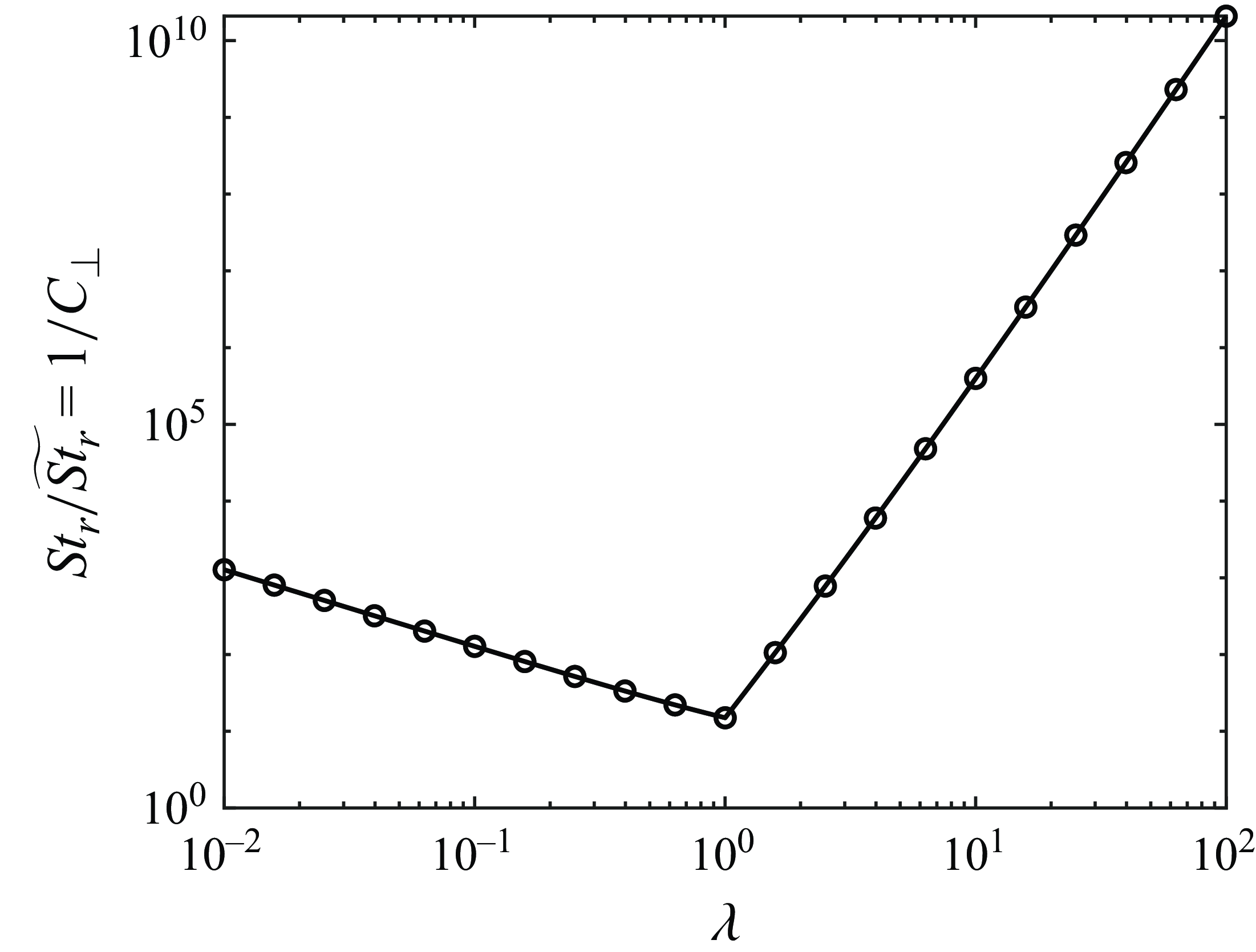
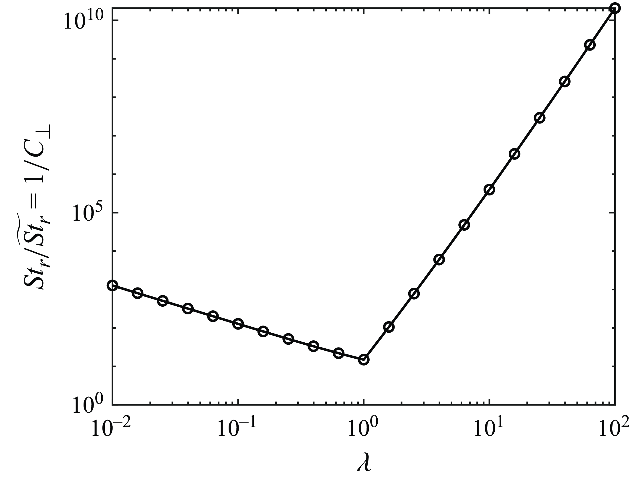
. To illustrate the relationship between these two Stokes numbers, we plot the factor
 $1/C_\perp$
, which is the scaling factor between
 $St_r$
and
 $\widetilde {St_r}$
, as a function of the aspect ratio
 $\lambda$
in figure 3. According to figure 3,
 $1/C_\perp$
increases exponentially as the aspect ratio
 $\lambda$
deviates from unity. This indicates that the amplitude of
 $St_r$
can be large even for a small value of
 $\widetilde {St_r}$
for particles with a shape deviating far away from a sphere. Nevertheless,
 $\widetilde {St_r}$
serves only as an approximate measure of particle inertia; thus, a large
 $\widetilde {St_r}$
indicates dominant particle-inertia effects, and vice versa. Hereinafter, we use
 $\widetilde {St_r}$
instead of
 $St_r C_\perp$
for the sake of the simplicity of the expression.
Relationship between
 $St_r/\widetilde {St_r}=1/C_\perp$
and aspect ratio
 $\lambda$
.
2.3. Equilibrium rotation modes of spheroids in shear flow
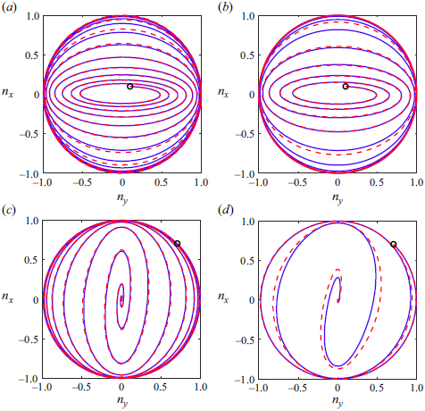
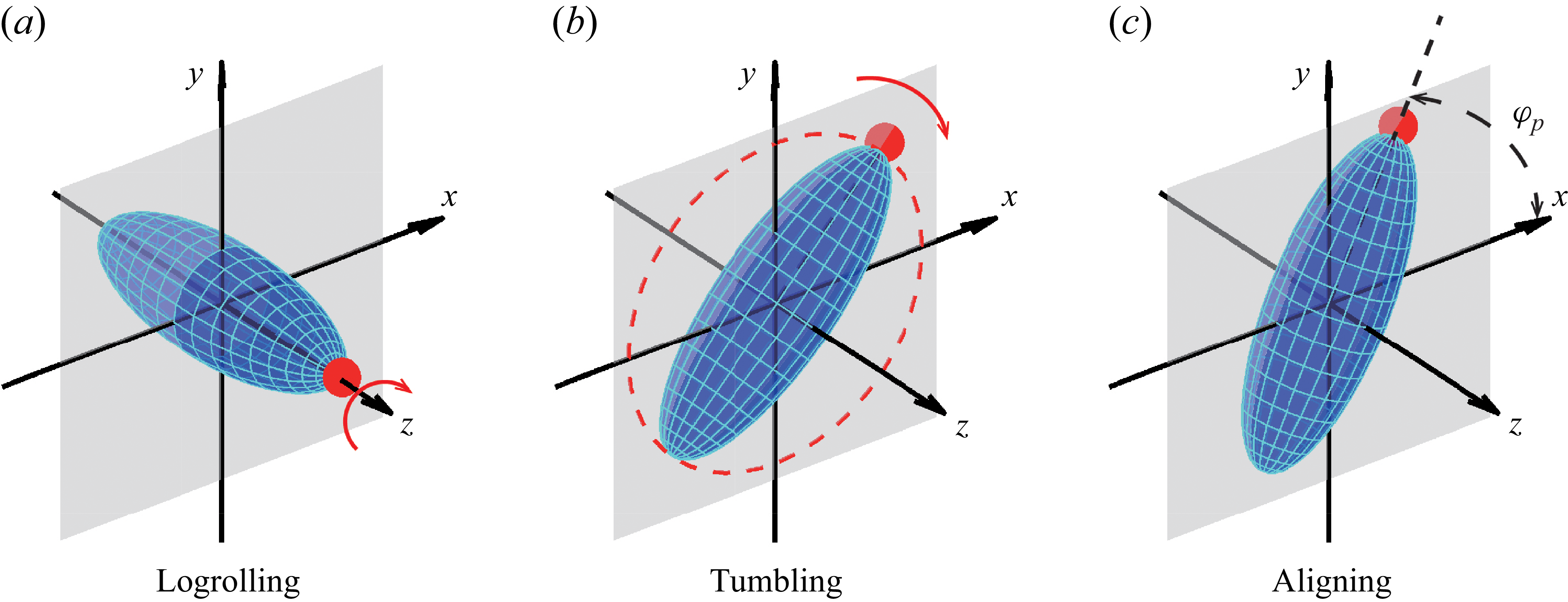
There are three equilibrium rotation modes of spheroids, i.e. logrolling, tumbling and aligning, as shown in figure 4. The transitional rotation modes are not considered in the current study. The logrolling mode signifies spheroids rotating about the symmetry axis, which orients to the vortical axis. The tumbling mode represents a spheroid rotating about its equatorial axis with its symmetry axis in the flow-gradient plane. The aligning mode means that the spheroid cannot rotate, but its symmetry axis keeps an angle relative to the streamwise direction.
Rotation modes of spheroids: (a) logrolling; (b) tumbling; (c) aligning.
For the logrolling, which is the simplest mode, the equilibrium state is
 $\boldsymbol n^e=[0,0,\pm 1]^T$
.
For the steady aligning mode, the corresponding orientation
 $\boldsymbol n^e$
is derived from (2.11) by setting
 $\boldsymbol \omega ^e=0$
and
 $({\mathrm{d}{\boldsymbol \omega ^e}}/{\mathrm{d}t})=0$
. Then (2.11) reduces to
 \begin{equation} \boldsymbol \varOmega =\boldsymbol n^e \times (\varLambda \unicode{x1D64E}+M\hat {\boldsymbol u}\hat {\boldsymbol u})\boldsymbol{\cdot }\boldsymbol n^e. \end{equation}
In the current shear flow,
 $\boldsymbol u=\kappa \!\boldsymbol y+\boldsymbol u_s$
, the aligning mode corresponds to the particle orientation vector
 $\boldsymbol n^e$
lying in the
 $x$
–
 $y$
plane. Under this condition, only the third component of the flow rotation
 $\boldsymbol \varOmega$
remains,
 \begin{equation} -\!\frac {1}{2}=-\frac {\varLambda }{2}{n^e_x}^2+Mn^e_x n^e_y+\frac {\varLambda }{2}{n^e_y}^2. \end{equation}
Meanwhile, the unit orientation vector
 $\boldsymbol n^e$
lying in the
 $x$
–
 $y$
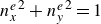
plane satisfies the constraint
 ${n^e_x}^2+{n^e_y}^2=1$
. By solving above equations, two pairs of solutions for
 $\boldsymbol n^e$
are obtained as follows:
 \begin{align} \left \{ \begin{aligned} {n^e_x}^2_{(1)}&=\dfrac {\varLambda ^2+M^2+\varLambda +\sqrt {\varLambda ^2M^2+M^4-M^2}}{2\varLambda ^2+2M^2} \\[4pt] {n^e_y}^2_{(1)}&=1-{n^e_x}^2_{(1)}=\dfrac {\varLambda ^2+M^2-\varLambda -\sqrt {\varLambda ^2M^2+M^4-M^2}}{2\varLambda ^2+2M^2}\nonumber \\ \end{aligned}\right . , \nonumber \\ \left \{ \begin{aligned} {n^e_x}^2_{(2)}&=\dfrac {\varLambda ^2+M^2+\varLambda -\sqrt {\varLambda ^2M^2+M^4-M^2}}{2\varLambda ^2+2M^2} \\[4pt]{n^e_y}^2_{(2)}&=1-{n^e_x}^2_{(2)}=\dfrac {\varLambda ^2+M^2-\varLambda +\sqrt {\varLambda ^2M^2+M^4-M^2}}{2\varLambda ^2+2M^2} \end{aligned}\right . . \end{align}
To be concise, the component
 $n_x^e$
is denoted as
 $p$
, leading to the following two solutions of
 $p$
satisfying
 \begin{align}& p_{(1)}^2=\frac {\varLambda ^2+M^2+\varLambda +\sqrt {\varLambda ^2M^2+M^4-M^2}}{2\varLambda ^2+2M^2},\nonumber \\ &p_{(2)}^2=\frac {\varLambda ^2+M^2+\varLambda -\sqrt {\varLambda ^2M^2+M^4-M^2}}{2\varLambda ^2+2M^2}. \end{align}
Finally, the equilibrium orientation
 $n^e$
of aligning mode satisfies
 \begin{equation} \boldsymbol n^e=\left[p, \frac {2\varLambda p^2-\varLambda -1}{2Mp},0\right]^T. \end{equation}
For each
 $p_{(1)}^2$
or
 $p_{(2)}^2$
, there is a pair of positive and negative values, representing two opposite vectors, i.e.
 $\boldsymbol n_+^e=-\boldsymbol n_{-}^e$
. Note that the subscripts ‘
 $+$
’ and ‘
 $-$
’ represent the directions computed by positive and negative
 $p$
, respectively. Because of the symmetry of the spheroid, the behaviours of the spheroid corresponding to these two vectors are identical.
Regarding tumbling, which is the most complicated mode, the equilibrium state is a periodic function with time in the flow-gradient plane, denoted as
 $\boldsymbol n^e(t)$
. According to Cui et al. (Reference Cui, Liu, Qiu and Zhao2024), when
 $\widetilde {St_r}$
is small, the non-dimensional period of tumbling rotation is
 $T_{p}^H=4\pi /\sqrt {1-\varLambda ^2-M^2}$
, while close to
 $T_{p}^L=4 \pi$
for large
 $\widetilde {St_r}$
. Moreover, around
 $\widetilde {St_r}\approx 1$
, the period of tumbling rotation transients from
 $T_{p}^H$
to
 $T_{p}^L$
. Meanwhile, when Stokes number
 $\widetilde {St_r}$
is non-zero, the periodic motions of the tumbling are only acquired numerically by solving a quasi-two-dimensional equation (Cui et al. Reference Cui, Liu, Qiu and Zhao2024), as expressed by
 \begin{equation} \widetilde {St_r}\frac {\mathrm{d}{\omega _z}}{\mathrm{d}t}=\frac {1}{2}\sqrt {\varLambda ^2+M^2}\cos (2\varphi +2\varphi _0)+\left(-\frac {1}{2}-\omega _z\right)\!, \end{equation}
where
 $2\varphi _0=\arctan (M/\varLambda )$
,
 $\omega _z$
and
 $\varphi$
are the angular velocity and displacement of a spheroid rotating in the flow-gradient plane, respectively. The details can be found in Cui et al. (Reference Cui, Liu, Qiu and Zhao2024). For finite
 $\widetilde {St_r}$
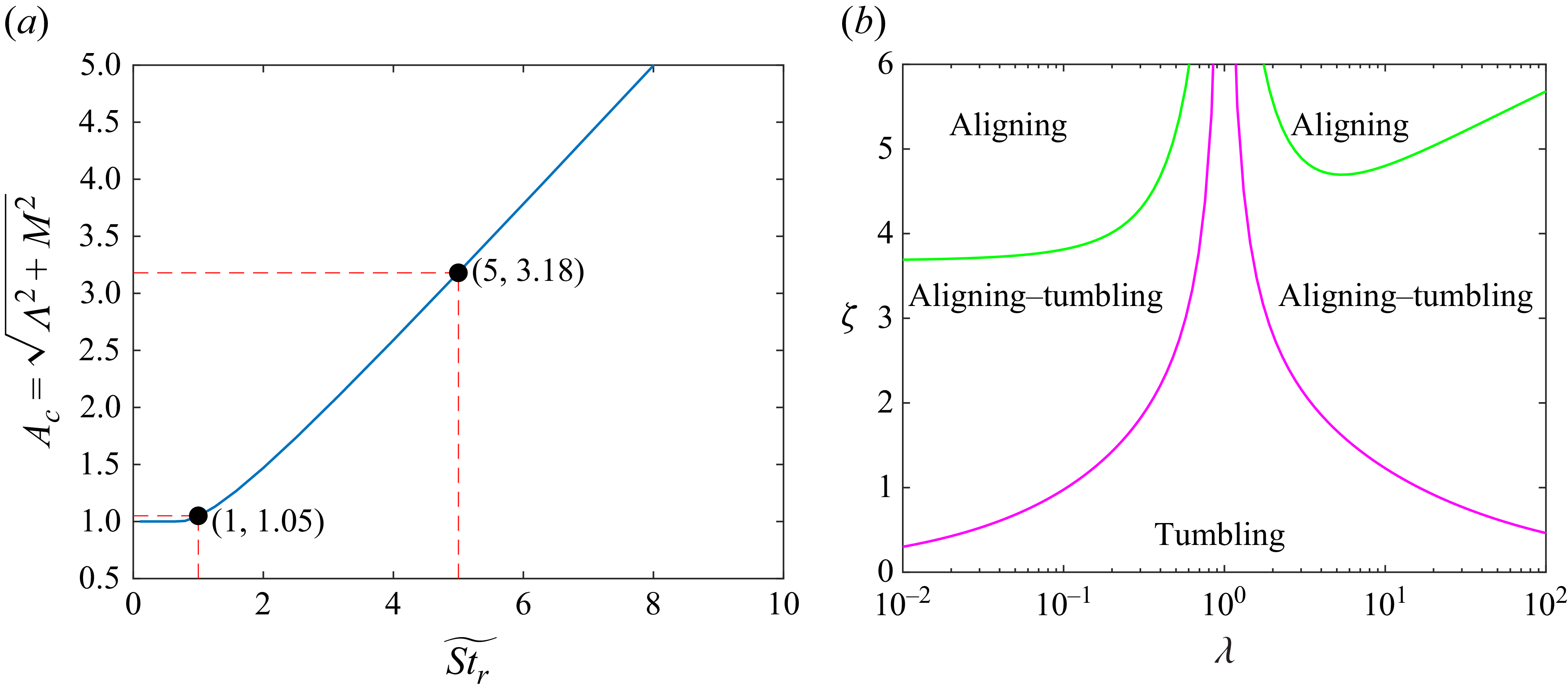
, there are no analytical solutions for the tumbling mode. Therefore, we primarily use numerical solutions of the tumbling mode as equilibrium states. Note that the tumbling mode always exists when
 $\varLambda ^2 + M^2 \lt 1$
. When
 $\varLambda ^2 + M^2 \geqslant 1$
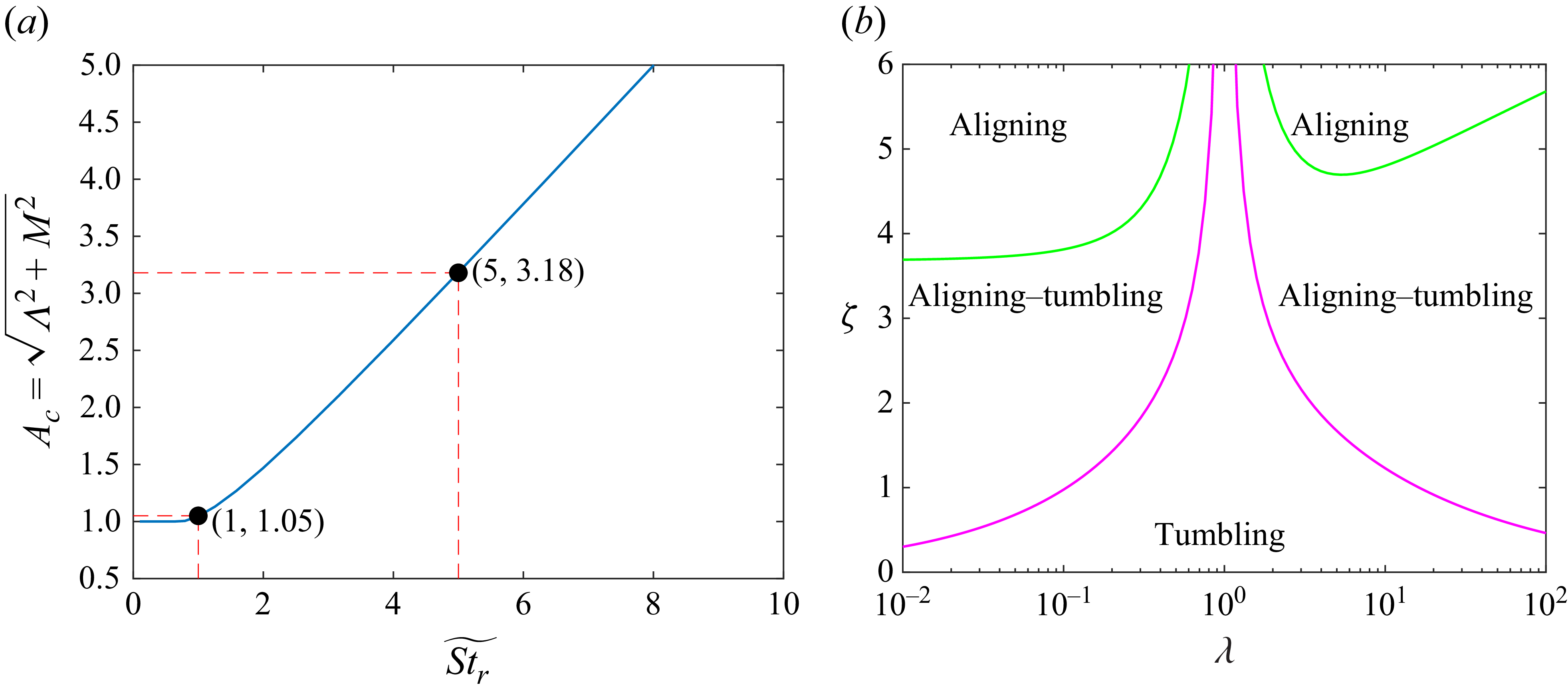
, the existence of the tumbling mode is no longer guaranteed. As shown in figure 5(a), there exists an upper critical value
 $A_c$
of
 $\sqrt {\varLambda ^2 + M^2}$
that depends on
 $\widetilde {St_r}$
. According to figure 5(b), when the parameter
 $\zeta$
exceeds the upper critical threshold, indicated by the green lines, only the aligning mode exists, regardless of the initial conditions. Conversely, when
 $\zeta$
falls below the magenta lines corresponding to
 $\varLambda ^2 + M^2 = 1$
, only the tumbling mode remains. Between the green and magenta lines, there is a transition region where both aligning and tumbling modes coexist. In this region, the final equilibrium state is sensitive to the initial conditions, including both the orientation and angular velocity of the spheroid.
(a) Upper critical values
 $A_c=\sqrt {\varLambda ^2+M^2}$
versus Stokes number
 $\widetilde {St_r}$
. (b) Regimes of equilibrium tumbling and aligning modes at
 $\widetilde {St_r}=5$
, where green lines represent
 $\varLambda ^2+M^2=3.18^2$
and magenta lines stand for
 $\varLambda ^2+M^2=1$
.
3. Linear stability analysis
In this study, we analyse the stability of spheroid rotation within two
 $\widetilde {St_r}$
ranges, namely
 $\widetilde {St_r}\ll 1$
and finite
 $\widetilde {St_r}$
. For
 $\widetilde {St_r} \ll 1$
, we use asymptotic theory based on the small parameter
 $\widetilde {St_r}$
to obtain an analytical expression of eigenvalues for stability (see (2.14)). This reflects how particle inertia affects the rotation of a weakly inertial spheroid. When
 $\widetilde {St_r}$
is finite, it is difficult to obtain analytical results (mostly there is no analytical solution). Therefore, a numerical stability analysis of spheroid rotation is conducted. In this section, the methods and results of linear stability analysis on different modes with
 $\widetilde {St_r}\ll 1$
and finite
 $\widetilde {St_r}$
are introduced as follows. Note that the following linear stability analysis only provides the insight of the particle behaviour close to the equilibrium state. If the particle initial condition is far away from these equilibrium states, nonlinear effects become dominant, and the predictions based on linear analysis become less accurate.
3.1. The case when
 $\widetilde {St_r}\ll 1$

When
 $\widetilde {St_r} \ll 1$
, (2.14) reflects the rotation motions of spheroids. In this section, (2.14) has the form of
 $({\mathrm{d}{\boldsymbol n}}/{\mathrm{d}t})= \mathcal{N}(\boldsymbol n)$
and the corresponding perturbation equation is
 $({\mathrm{d}{\delta \boldsymbol n}}/{\mathrm{d}t})=({\partial }/{\partial \boldsymbol n}) \mathcal{N}(\boldsymbol n^e)\boldsymbol{\cdot }\delta \boldsymbol n$
, where
 $\boldsymbol n^e$
represents an orientation of equilibrium state and
 $({\partial }/{\partial \boldsymbol n}) \mathcal{N}(\boldsymbol n^e)$
refers to a stability matrix, denoted as
 $\unicode{x1D64C}(\boldsymbol n^e)$
. Due to the constraint
 $n_x^2+n_y^2+n_z^2=1$
, the three-dimensional orientational dynamics of the particle are effectively reduced into a two-dimensional system in
 $(n_x, n_y)$
subspace by substituting
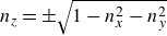 $n_z=\pm \sqrt {1-n_x^2-n_y^2}$
into the orientational dynamics equations, i.e.
 \begin{equation} \frac {\mathrm{d}{}}{\mathrm{d}t} \left [\begin{matrix} n_x\\n_y\\ \end{matrix}\right ]=\mathcal{N}(n_x,n_y), \end{equation}
For logrolling and aligning states,
 $\boldsymbol n^e$
is independent of time, resulting in a constant stability matrix
 $\unicode{x1D64C}$
. Therefore, we can use a stability theory of fixed points to analyse logrolling and aligning modes. However, the tumbling modes are periodic with time, which should be analysed by Floquet theory (Joseph Reference Joseph1976; Chicone Reference Chicone2006).
3.1.1. Logrolling mode
For the logrolling mode, the orientation of the spheroid is
 $\boldsymbol n^e=[0,0,\pm 1]^T$
. The perturbation equation of logrolling mode is
 \begin{equation} \frac {\mathrm{d}{}}{\mathrm{d}t}\left [\begin{matrix} \delta n_x\\\delta n_y\\ \end{matrix}\right ]=\left [\begin{matrix} \dfrac {\left(-\varLambda ^2-2M^2+\varLambda \right)\widetilde {St_r}}{2}+M & -\dfrac {(1+\varLambda )\left(M\widetilde {St_r}-1\right)}{2}\\[8pt] -\dfrac {1}{2}+\dfrac {\varLambda }{2}&0\\ \end{matrix}\right ]\left [\begin{matrix} \delta n_x\\ \delta n_y\\ \end{matrix}\right ]\!. \end{equation}
Consequently, the eigenvalues of the corresponding stability matrix
 $\unicode{x1D64C}$
are shown as follows:
 \begin{align} b_{1,2}&=\frac {M}{2}+\widetilde {St_r} \frac {\left(-\varLambda ^2-2M^2+\varLambda \right)}{4}\nonumber\\ &\quad \pm \frac {\sqrt {(2M^2+\varLambda ^2-\varLambda )^2\widetilde {St_r}^2-4(2M^2+2\varLambda ^2-\varLambda -1)M \widetilde {St_r}+4M^2+4\varLambda ^2-4}}{4}\nonumber\\ &\quad +O\left(\widetilde {St_r}^2\right)\!, \end{align}
where the signs of
 $b_{1,2}$
determine the stability of the logrolling mode. When
 $\widetilde {St_r}=0$
, (3.3) degenerates into
 \begin{align} &b_{1,2}=\frac {M}{2}\pm \frac {\sqrt {M^2+\varLambda ^2-1}}{2}, \end{align}
which is consistent with the results in Cui et al. (Reference Cui, Liu, Qiu and Zhao2024). For prolate spheroids, when the fluid-inertial torque is considered,
 $M$
is negative, and the maximum real part of
 $b_{1,2}$
is also negative, reflecting that the logrolling of the prolate spheroid is stable. For oblate spheroids,
 $M$
is positive, and the maximum real part of
 $b_{1,2}$
is positive, indicating that the logrolling of an oblate spheroid is unstable. Note that
 $\varLambda ^2$
is linked to shape and is always below unity. When particle inertia is taken into consideration, the stability map changes with increasing
 $\widetilde {St_r}$
and varying
 $\zeta$
, as depicted in figure 6. For
 $\widetilde {St_r}=0.1$
(see figure 6
a), the logrolling mode for prolate spheroids is unstable but it is stable for oblate spheroids when
 $\zeta$
is small. It is obvious that the critical
 $\zeta _c$
for neutral stability of thin oblate ones is nearly independent of
 $\lambda$
and larger than that of prolate ones, which is attributed to the nearly constant and large
 $F_\lambda$
for oblate spheroids. Meanwhile, the critical
 $\zeta _c$
decreases as the aspect ratio
 $\lambda$
increases for prolate spheroids. This indicates that the stability of the logrolling of the prolate spheroids is easily affected by the fluid-inertial torque from stable state to unstable state, but for the oblate spheroids,
 $\zeta _c$
is relatively higher. At the same time, for the fixed aspect ratios, e.g.
 $\lambda =0.1$
and
 $10$
as shown in figure 6(b), the critical
 $\zeta _c$
and
 $\widetilde {St_r}$
exhibit a power-law relationship
 $\widetilde {St_r}\sim \zeta _c^2$
, indicating that as particle inertia increases, a larger fluid-inertial torque is required to overcome the effect of the particle inertia.
Stability of the logrolling of spheroidal particle computed by (3.3). (a) The maximum real parts of eigenvalues
 $b_{1,2}$
with different
 $\zeta$
and
 $\lambda$
at
 $\widetilde {St_r}=0.1$
, and (b) boundaries between stable and unstable regions of spheroids versus particle inertia
 $\widetilde {St_r}$
within
 $0\sim 0.5$
for
 $\lambda =0.1$
(solid line) and
 $\lambda =10$
(dashed line). In panel (a), solid lines represent zero value, and magenta dashed–dotted lines represent
 $\varLambda ^2+M^2=1$
. Note that when the maximum real part of the eigenvalue is negative, the logrolling mode is stable, and vice versa. Here ‘US’ and ‘S’ represent unstable and stable states, respectively.

3.1.2. Aligning mode
The aligning mode only exists when
 $A^2=M^2+\varLambda ^2\geqslant 1$
, and there are two pairs of orientations referring to the equilibrium states. The first pair satisfies
 $p_{(1)}^2= ({\varLambda ^2+M^2+\varLambda +\sqrt {\varLambda ^2M^2+M^4-M^2}})/({2\varLambda ^2+2M^2})$
, and the corresponding eigenvalues of the stability matrix
 $\unicode{x1D64C}$
are
 \begin{align} b_1= & -\frac {M^2-|M|M +2\sqrt {\varLambda ^2M^2 + M^4 - M^2}}{2M} \nonumber \\ & -\frac {\widetilde {St_r}}{4} \left [\frac {3\varLambda ^2M + \varLambda ^2|M|+ 4M^3 - 3M - |M|}{M}\right . \nonumber \\ &\left .+\frac { (2M-|M|)\sqrt {\varLambda ^2M^2 + M^4 - M^2}}{M}\right ]+O\big(\widetilde {St_r}^2\big), \end{align}
 \begin{align} b_2= & -\frac {M^2+|M|M +2\sqrt {\varLambda ^2M^2 + M^4 - M^2}}{2M} \nonumber \\ & -\frac {\widetilde {St_r}}{4}\left [\frac {3\varLambda ^2M-\varLambda ^2|M|+ 4M^3 - 3M + |M|}{M}\right . \nonumber \\ &\left . +\frac { (2M+|M|)\sqrt {\varLambda ^2M^2 + M^4 - M^2}}{M}\right ]+O\big(\widetilde {St_r}^2\big). \end{align}
For the second one,
 $p_{(2)}^2=({\varLambda ^2+M^2+\varLambda -\sqrt {\varLambda ^2M^2+M^4-M^2}})/({2\varLambda ^2+2M^2})$
, and the corresponding eigenvalues of the stability matrix
 $\unicode{x1D64C}$
are
 \begin{align} b_1= & -\frac {M^2-|M|M -2\sqrt {\varLambda ^2M^2 + M^4 - M^2}}{2M} \nonumber \\ & -\frac {\widetilde {St_r}}{4} \left [\frac {3\varLambda ^2M + \varLambda ^2|M|+ 4M^3 - 3M - |M|}{M}\right . \nonumber \\ &\left .-\frac { (2M-|M|)\sqrt {\varLambda ^2M^2 + M^4 - M^2}}{M}\right ]+O\big(\widetilde {St_r}^2\big), \end{align}
 \begin{align} b_2= & -\frac {M^2+|M|M -2\sqrt {\varLambda ^2M^2 + M^4 - M^2}}{2M} \nonumber \\ & -\frac {\widetilde {St_r}}{4}\left [\frac {3\varLambda ^2M-\varLambda ^2|M|+ 4M^3 - 3M + |M|}{M}\right . \nonumber \\ &\left . -\frac { (2M+|M|)\sqrt {\varLambda ^2M^2 + M^4 - M^2}}{M}\right ]+O\big(\widetilde {St_r}^2\big). \end{align}
The stability of the aligning mode is shown in the regions of
 $\varLambda ^2+M^2\geqslant 1$
in figure 7(a) at
 $\widetilde {St_r}=0.1$
. A stable aligning mode for oblate spheroids and an unstable align mode for prolate ones at small Stokes number with a pronounced slip velocity are observed, which explains why we can only observe the aligning mode for oblate spheroids instead of prolate ones at small
 $\widetilde {St_r}$
in our previous PP simulation results (Cui et al. Reference Cui, Liu, Qiu and Zhao2024).
Stability of the aligning (in
 $\varLambda ^2+M^2\geqslant 1$
) and the tumbling (in
 $\varLambda ^2+M^2\lt 1$
) of spheroidal particle computed by (3.5)–(3.7) and (3.14). (a) The maximum real parts of eigenvalues in (3.5–3.7) and the values of Floquet exponent in (3.14) with different
 $\zeta$
and
 $\lambda$
at
 $\widetilde {St_r}=0.1$
, and (b) boundaries between stable and unstable regions of spheroids versus particle inertia
 $\widetilde {St_r}$
within
 $0\sim 0.5$
for
 $\lambda =0.1$
(solid line) and
 $\lambda =10$
(dashed line). In panel (a), solid lines represent zero values, and magenta dashed–dotted lines represent
 $\varLambda ^2+M^2=1$
. Note that when the contour values shown in (a) are negative, the corresponding rotation mode is stable, and vice versa. Here ‘US’ and ‘S’ represent unstable and stable states, respectively.
3.1.3. Tumbling mode
For the tumbling mode (
 $M^2+\varLambda ^2\lt 1$
), the equilibrium motion of
 $\boldsymbol n^e$
is a periodic function with the time. Inspired by the study of Einarsson et al. (Reference Einarsson, Angilella and Mehlig2014), analytical solutions of the eigenvalues of the stability matrix are conducted via Floquet theory with
 $\widetilde {St_r} \ll 1$
. By substituting unit vector
 $\boldsymbol n=[\sin \vartheta \cos \varphi ,\sin \vartheta \sin \varphi ,\cos \vartheta ]$
into (2.14), the orientational dynamics of the spheroid is expressed by
 \begin{align} \frac {\mathrm{d}{\varphi }}{\mathrm{d}t}= & f(\varphi ,\vartheta ) \nonumber \\ = & \frac {1}{2}(-1+\varLambda \cos 2\varphi -M\sin 2\varphi )+\frac {\widetilde {St_r}}{8}\lbrace [2M^2\sin 2\varphi \nonumber \\ & -M(\varLambda -1)\cos 2\varphi +M^2\sin 4\varphi -M(2\varLambda \cos 4\varphi -\varLambda -1)]\cos 2\vartheta \nonumber \\ & +2M^2\sin 2\varphi -M(\varLambda +3)\cos 2\varphi -M^2\sin 4\varphi \nonumber \\ & +M(2\varLambda \cos 4\varphi +\varLambda +1)+2\varLambda ^2\sin 4\varphi \sin ^2\vartheta \nonumber \\ & +\sin 2\varphi [\varLambda (\varLambda +1)\cos 2\vartheta +\varLambda ^2-3\varLambda ]\rbrace +O\big(\widetilde {St_r}^2\big), \end{align}
 \begin{align} \frac {\mathrm{d}{\vartheta }}{\mathrm{d}t}= &\, g(\varphi ,\vartheta ) \nonumber \\ = & \sin \vartheta \cos \vartheta \cos \varphi (M\cos \varphi +\varLambda \sin \varphi ) \nonumber \\ & + \widetilde {St_r}\sin \vartheta \cos \vartheta \cos ^2\varphi \left \lbrace 2 M^2\sin ^2\vartheta \cos ^2\varphi \vphantom{\frac {\varLambda }{2}}\right . \nonumber \\ & +4M\varLambda \sin \varphi \cos \varphi \sin ^2\vartheta -M^2-\frac {M(\varLambda +1)}{2}\tan \varphi \nonumber \\ &\left . +\,2\varLambda ^2\sin ^2\vartheta \sin ^2\varphi -\frac {\varLambda ^2}{2}+\frac {\varLambda }{2}\right \rbrace +O\big(\widetilde {St_r}^2\big). \end{align}
Here,
 $\varphi$
denotes the relative angle between the x-axis and the projection of
 $\boldsymbol n$
in the x–y plane, while
 $\vartheta$
represents the angle of
 $\boldsymbol n$
with respect to the vortical axis, i.e. z-axis. According to (3.9), the evolution of
 $\varphi$
and
 $\vartheta$
are decoupled only if
 $\widetilde {St_r}=0$
. However, the presence of particle inertia makes
 $\varphi$
and
 $\vartheta$
coupled with each other, leading to a strong nonlinearity. When a spheroid is tumbling in the x–y plane, its equilibrium
 $\vartheta _0=\pi /2$
, while
 $\varphi _0(t)$
is a periodic function with a period
 $T_{\!p}=4\pi /\sqrt {1-\varLambda ^2-M^2}$
when
 $\widetilde {St_r}\ll 1$
(Cui et al. Reference Cui, Liu, Qiu and Zhao2024). By considering small perturbations on the equilibrium, i.e.
 $\vartheta =\vartheta _0+\delta \vartheta$
and
 $\varphi (t)=\varphi _0(t)+\delta \varphi (t)$
, the corresponding linear perturbation equation of
 $\delta \vartheta$
is
 \begin{equation} \frac {\mathrm{d}{}}{\mathrm{d}t}\delta \vartheta =\delta \vartheta \frac {\partial g}{\partial \vartheta }\Bigg|_{(\varphi _0(t),\vartheta _0)}+\delta \varphi \frac {\partial g}{\partial \varphi }\Bigg|_{(\varphi _0(t),\vartheta _0)}. \end{equation}
When
 $\vartheta _0=\pi /2$
,
 $g$
is independent of
 $\varphi$
, namely
 $({\partial g}/{\partial \varphi })=0$
. Hence, the above equation is simplified to
 \begin{equation} \frac {\mathrm{d}{}}{\mathrm{d}t}\ln \delta \vartheta =\left . \frac {\partial g}{\partial \vartheta }\right|_{(\varphi _0(t),\vartheta _0)}. \end{equation}
According to the Floquet theory, we integrate (3.12) along the trajectory (
 $\varphi _0, \vartheta _0$
) with a period
 $T_{\!p}$
and average the Floquet exponent by
 $T_{\!p}$
, i.e.
 \begin{equation} \gamma _{\pi /2}=\frac {1}{T_{\!p}}\int _0^{T_{\!p}}{\rm d}t\frac {\partial g}{\partial \vartheta }\Bigg|_{(\varphi _0(t),\vartheta _0)}=-\frac {1}{T_{\!p}}\int _0^{2\pi }\frac {{\rm d} \varphi }{\dot \varphi }\frac {\partial g}{\partial \vartheta }\Bigg|_{(\varphi _0(t),\vartheta _0)}. \end{equation}
Here,
 $\dot {\varphi }={\mathrm{d}{\varphi }}/{\mathrm{d}t}$
. After integrating above equation and retaining the first-order term of
 $\widetilde {St_r}$
, the Floquet exponent
 $\gamma _{\pi /2}$
of the tumbling mode is expressed as
 \begin{equation} \gamma _{\pi /2}=-\frac {M}{2}+\frac {\widetilde {St_r}}{4}\left [M^2+\varLambda ^2+(1-\varLambda )\sqrt {1-M^2-\varLambda ^2}-1\right ]+O\big(\widetilde {St_r}^2\big). \end{equation}
When
 $\gamma _{\pi /2}\lt 0$
, the tumbling mode is stable and vice versa. When
 $M=0$
, the simplified form of (3.14) is consistent with the results reported in Einarsson et al. (Reference Einarsson, Angilella and Mehlig2014). The corresponding results of (3.14) are shown in figure 7. When the fluid inertia effect is weaker than the particle inertia effect, the tumbling of prolate spheroids is stable but not for oblate ones. Contrarily, when the fluid inertia effect is greater than the particle inertia effect, the tumbling of prolate spheroids becomes unstable, but that of the oblate spheroids becomes stable. These results are consistent with our previous simulations (Cui et al. Reference Cui, Liu, Qiu and Zhao2024). Besides, for fixed aspect ratios, such as
 $\lambda =0.1$
and
 $10$
, the critical
 $\zeta _c$
for neutral stability still shows
 $\widetilde {St_r}\sim \zeta _c^2$
with
 $\widetilde {St_r}\ll 1$
, as depicted in figure 7(b).
Meanwhile, the Floquet exponent
 $\gamma _{\pi /2}$
indicates the rate at which perturbed trajectories converge to or diverge from the tumbling equilibrium mode. A Floquet exponent with a value close to zero indicates a slow convergence (negative exponent) or divergence (positive exponent) and vice versa. According to (3.14), the Floquet exponents associated with the tumbling modes at
 $\zeta =0$
fall within the range
 $[-0.08,0.18] \widetilde {St_r}$
, which are one to two orders of magnitude smaller than
 $\widetilde {St_r}$
(Einarsson et al. Reference Einarsson, Angilella and Mehlig2014). This indicates that, for small
 $\widetilde {St_r}$
, the evolution of perturbations near the tumbling mode is slow. Note that an
 $O(1)$
or smaller value of
 $\widetilde {St_r}$
may correspond to a large
 $St_r$
for extreme aspect ratios. These findings are similar to those of Dabade et al. (Reference Dabade, Marath and Subramanian2016), although their study focused exclusively on neutrally buoyant spheroids, whereas the present work investigates spheroids with a sufficiently large particle-to-fluid density ratio.
3.2. Finite
$\widetilde {St_r}$

When
 $\widetilde {St_r}$
is finite, such as
 $\widetilde {St_r}\sim 1$
or
 $\widetilde {St_r}\gt 1$
, the weakly inertial form of the orientational dynamics of the spheroid (see (2.14)) becomes invalid. For finite
 $\widetilde {St_r}$
, the stability analysis should be performed based on (2.11), whose perturbation equation is of the following form:
 \begin{equation} \frac {\mathrm{d}{}}{\mathrm{d}t}\left [\begin{matrix} \delta \boldsymbol n \\ \delta \boldsymbol \omega \\ \end{matrix}\right ] = \unicode{x1D64C}\boldsymbol{\cdot }\left [\begin{matrix} \delta \boldsymbol n \\ \delta \boldsymbol \omega \\ \end{matrix}\right ]\!. \end{equation}
Here,
 $\delta \boldsymbol n$
and
 $\delta \boldsymbol{\omega}$
are the perturbations of orientation and angular velocity, respectively. Here
 $\unicode{x1D64C}$
is the stability matrix related to
 $\boldsymbol n^e$
and
 $\boldsymbol \omega ^e$
. According to Cui et al. (Reference Cui, Liu, Qiu and Zhao2024), the boundary of the equilibrium aligning and the tumbling modes is vague due to the particle inertia, i.e. near
 $A^2=M^2+\varLambda ^2=1$
spheroids may align or continuously tumble depending on initial conditions. Consequently, it is difficult to determine the boundaries for only the aligning mode or tumbling mode directly. Nevertheless, the aligning mode can be thought of a special tumbling mode with an infinitely long period. In this way, we can simplify aligning mode and tumbling mode into one case. Therefore, we just discuss the stability of logrolling, and tumbling–aligning modes.
3.2.1. Logrolling mode
For the logrolling mode,
 $\boldsymbol n^e=[0,0,\pm 1]^T$
. Due to the constraint for the unit vector
 $\boldsymbol n$
, the perturbation along
 $z$
direction
 $\delta n_z$
near the logrolling mode
 $\boldsymbol n^e$
is zero, i.e.
 $\delta n_z =-n_x^e/n_z^e\delta n_x-n_y^e/n_z^e\delta n_y=0$
. Therefore,
 $\delta \boldsymbol n$
only has the components of
 $\delta n_x$
and
 $\delta n_y$
, and the corresponding perturbation equations with constant coefficients are divided into two independent equation sets, i.e.
 \begin{align}& \frac {\mathrm{d}{ }}{\mathrm{d}t}\left [\begin{matrix} \delta \omega _x \\ \delta \omega _y \\ \delta n_x \\ \delta n_y \end{matrix}\right ] =\left [\begin{matrix} -\dfrac {1}{St_r C_\perp } & \dfrac {\varLambda }{2} & -\dfrac {\varLambda }{2St_r C_\perp } & -\dfrac {\varLambda }{4} \\[10pt] \dfrac {\varLambda }{2} & -\dfrac {1}{St_r C_\perp } & \dfrac {\varLambda }{4}+\dfrac {M}{St_r C_\perp } & \dfrac {\varLambda }{2St_r C_\perp } \\[10pt] 0 & 1 & 0 & \dfrac {1}{2} \\[10pt] -1 & 0 & -\dfrac {1}{2} & 0 \end{matrix}\right ] \left [\begin{matrix} \delta \omega _x \\ \delta \omega _y \\ \delta n_x \\ \delta n_y \end{matrix}\right ]\!, \end{align}
 \begin{align}&\qquad\qquad\qquad\qquad\qquad\qquad \frac {\mathrm{d}{\delta \omega _z}}{\mathrm{d}t} =-\frac {1}{St_rC_\parallel }\delta \omega _z . \end{align}
Here, (3.17) has a negative eigenvalue
 $-1/(St_rC_\parallel )$
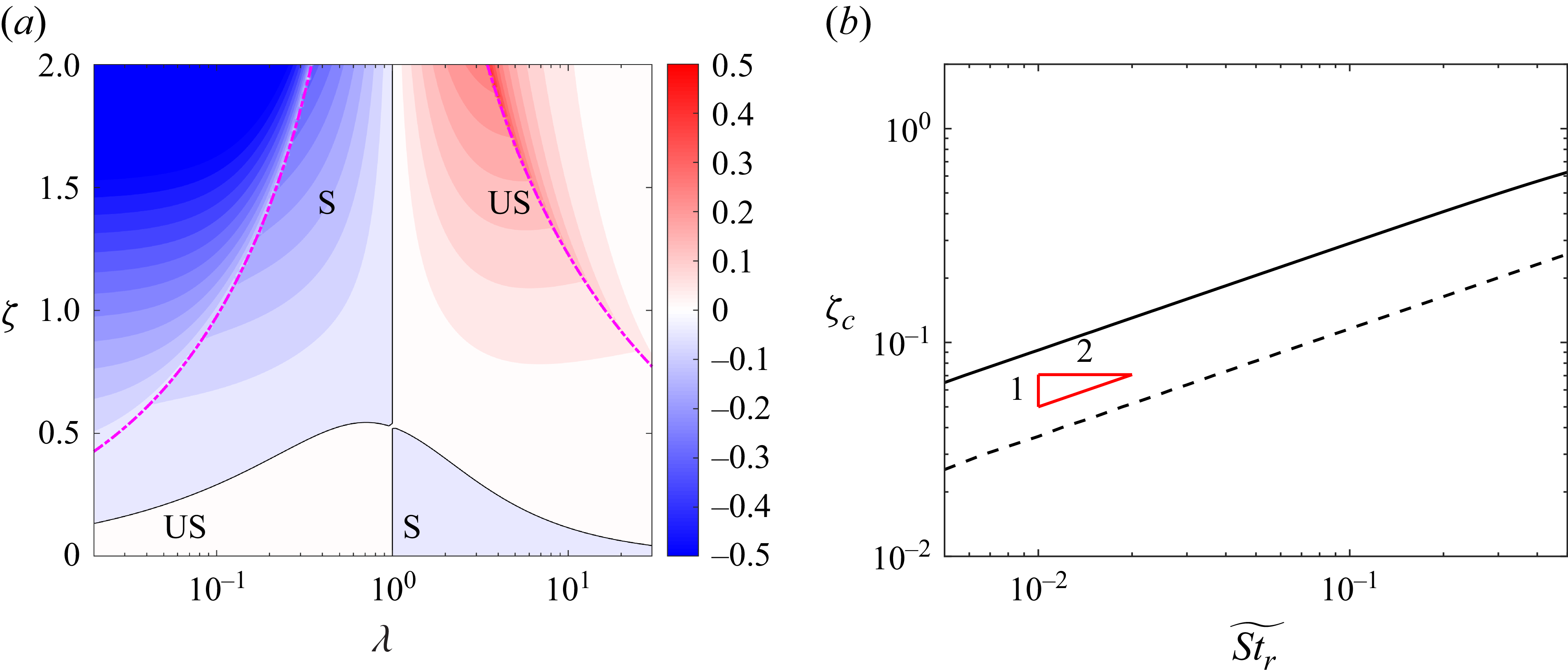
, and, therefore, only (3.16) are viewed as primary perturbation equations to reflect the stability of the logrolling mode. The real part of the maximum eigenvalue of the stability matrix in (3.16), denoted as
 $\xi _m$
, serves as the criterion for the stability. The distributions of
 $\xi _m$
with different Stokes numbers, aspect ratios and
 $\zeta$
are shown in figure 8. Similar to the weakly inertial results, the black lines for the neutral stable logrolling mode rise with increasing particle inertia, reflecting that greater fluid inertia is needed to overcome the effect of particle inertia.
Stability of the logrolling mode of the spheroidal particle computed by (3.16) with (a)
 $\widetilde {St_r}=1$
and (b)
 $\widetilde {St_r}=5$
. Here, black solid lines represent zero value of eigenvalues representing boundaries between stable and unstable regions, and magenta dashed–dotted lines represent
 $\varLambda ^2+M^2=1$
. Here ‘US’ and ‘S’ represent unstable and stable states, respectively.

3.2.2. Aligning and tumbling modes
Regarding the aligning and the tumbling modes in the flow-gradient plane, the primary perturbation equation is
 \begin{equation} \frac {\mathrm{d}{ }}{\mathrm{d}t}\left [\begin{matrix} \delta \omega _x \\ \delta \omega _y \\ \delta n_z \end{matrix}\right ] =\unicode{x1D64C}(\boldsymbol \omega ^e(t),\boldsymbol n^e(t)) \left [\begin{matrix} \delta \omega _x \\ \delta \omega _y \\ \delta n_z \end{matrix}\right ]\!, \end{equation}
where the components of the stability matrix
 $\unicode{x1D64C}$
are listed as
 \begin{align} Q_{11} & =\left(\frac {1}{St_r C_\perp }-\frac {1}{St_r C_\parallel }\right){n_x^e}^2-\varLambda n_x^e n_y^e \omega _z^e-\frac {1}{St_r C_\perp }, \nonumber \\ Q_{12} & =-\varLambda {n_y^e}^2\omega _z^e+\left(\frac {1}{St_r C_\perp }-\frac {1}{St_r C_\parallel }\right)n_x^e n_y^e, \nonumber \\ Q_{13} & =-\frac {\varLambda }{2St_r C_\perp }n_x^e+\left(\frac {1}{St_r C_\perp }-\frac {1}{St_r C_\parallel }\right)\left(\omega _z^e+\frac {1}{2}\right)n_x^e-\varLambda n_y^e {\omega _z^e}^2, \nonumber \\ Q_{21} & =\varLambda {n_x^e}^2\omega _z^e+\left(\frac {1}{St_r C_\perp }-\frac {1}{St_r C_\parallel }\right)n_x^e n_y^e, \nonumber \\ Q_{22} & =\left(\frac {1}{St_r C_\perp }-\frac {1}{St_r C_\parallel }\right){n_y^e}^2+\varLambda n_x^e n_y^e \omega _z^e-\frac {1}{St_r C_\perp }, \nonumber \\ Q_{23} & =\frac {\varLambda }{2St_r C_\perp }n_y^e+\left(\frac {1}{St_r C_\perp }-\frac {1}{St_r C_\parallel }\right)\left(\omega _z^e+\frac {1}{2}\right)n_y^e+\varLambda n_y^e {\omega _z^e}^2+\frac {M}{St_r C_\perp }n_x^e, \nonumber \\ Q_{31} & =n_y^e,\qquad Q_{32}=-n_x^e,\qquad Q_{33}=0. \end{align}
Other independent equation set of perturbation equations is
 \begin{equation} \frac {\mathrm{d}{}}{\mathrm{d}t}\left [\begin{matrix} \delta \omega _z \\ \delta n_x \\ \delta n_y \end{matrix}\right ] = \left [\begin{matrix} -\dfrac {1}{St_r C_\perp } & \dfrac {\varLambda }{St_r C_\perp }n_x^e-\dfrac {M}{St_r C_\perp }n_y^e & \dfrac {\varLambda }{St_r C_\perp }n_y^e-\dfrac {M}{St_r C_\perp }n_x^e \\[10pt] -n_y^e & 0 & -\omega _z^e \\[6pt] n_x^e & \omega _z^e & 0 \\ \end{matrix}\right ] \left [\begin{matrix} \delta \omega _z \\ \delta n_x \\ \delta n_y \end{matrix}\right ]\!, \end{equation}
which only characterizes the stability of the aligning and tumbling modes confined to the flow-gradient plane, but does not capture departures of the spheroid orientation from the flow-gradient plane. Therefore, we consider the stability of (3.18). According to our previous study (Cui et al. Reference Cui, Liu, Qiu and Zhao2024), the rotation modes in the flow-gradient plane for the spheroids with finite Stokes number depend on the initial orientations and angular velocities within certain ranges of
 $\sqrt {\varLambda ^2+M^2}, \widetilde {St_r}$
and
 $\zeta$
. Nevertheless, those results in Cui et al. (Reference Cui, Liu, Qiu and Zhao2024) were obtained without perturbations along the vortical axis. In this study, differing from the quasi-two-dimensional results, the perturbations along the vortical axis are considered. Nevertheless, we still reckon the aligning and tumbling modes in the flow-gradient plane are two equilibria of spheroids in three-dimensional cases. However, it is unfeasible to compute (2.20) by traversing all initial values. To acquire final rotation modes as fast as possible, similar to Cui et al. (Reference Cui, Liu, Qiu and Zhao2024), we set
 $(\omega _z=0, \varphi +\varphi _0=0)$
and
 $(\omega _z=-0.5, \varphi +\varphi _0=\pi /2)$
as initial values to obtain time series of spheroids orientations and angular velocities by (2.20). After that, by using Floquet theory numerically, as shown in Appendix C, we can attain a maximum eigenvalue
 ${\varrho }_m$
as a criterion for stability. Note that although the aligning mode is not periodic, we can still use Floquet theory by considering the period of the aligning mode set as any non-zero values. The phase diagrams of the stability of the tumbling and the aligning modes are shown in figure 9. When using the initial values
 $(\omega _z=0, \varphi +\varphi _0=0)$
, the corresponding equilibrium is the aligning mode with
 $M^2+\varLambda ^2\geqslant 1$
, as shown in figure 9(a,b), suggesting stable aligning modes for oblate spheroids and unstable aligning modes for prolate ones. In figure 9(c,d), the results are obtained using initial conditions
 $(\omega _z=-0.5, \varphi +\varphi _0=\pi /2)$
within the region defined by
 $M^2+\varLambda ^2\lt A_c^2$
(tumbling mode), where the critical value are
 $A_c=1.05$
at
 $\widetilde {St_r}=1$
and
 $A_c=3.18$
at
 $\widetilde {St_r}=5$
. The stability is determined by the relative importance of fluid inertia to particle inertia. For small
 $\zeta$
, namely a weak fluid inertia effect compared with particle inertia, the tumbling mode for oblate spheroids is unstable but remains stable for prolate spheroids. As
 $\zeta$
increases, for moderate aspect ratios close to unit, the tumbling mode becomes stable for oblate spheroids while unstable for prolate spheroids. Note that as particle inertia increases, the critical
 $\zeta _c$
, which separates the stable and unstable regimes for the tumbling mode, also increases.
Stability of (a,b) the aligning and (c,d) the tumbling modes of spheroidal particle computed by (3.18) with finite Stokes numbers (a,c)
 $\widetilde {St_r}=1$
and (b,d)
 $\widetilde {St_r}=5$
. Note that the contour represents Floquet exponent
 $\gamma _m =\ln (\varrho _m)/T_{\!p}$
. The equilibrium rotations in the x–y plane are obtained by numerically integrating (2.20). (a,b) The aligning mode is obtained by using the initial condition (
 $\omega _z=0, \varphi +\varphi _0=0$
), (c,d) while the tumbling mode is evaluated using (
 $\omega _z=-0.5, \varphi +\varphi _0=\pi /2$
) as initial values. Black solid lines represent
 $\gamma _m=0$
, and magenta dashed–dotted lines represent
 $\varLambda ^2+M^2=1$
. The green solid lines in (a) and (c) represent
 $\varLambda ^2+M^2=1.05^2$
and in (b) and (d) represent
 $\varLambda ^2+M^2=3.18^2$
. Between the green and magenta lines lies a coexistence regime, where both aligning and tumbling modes are possible, and the final state depends sensitively on the initial orientation and angular velocity. Here ‘US’ and ‘S’ represent unstable and stable states, respectively.

3.3. Phase diagrams of stable rotations of spheroids
To summarize, we integrate all stable modes into phase diagrams with
 $\widetilde {St_r}=0$
, 0.1, 1 and 5 and the aspect ratios
 $\lambda$
ranging from
 $0.02$
to
 $30$
, as shown in figure 10. Note that the results of
 $\widetilde {St_r}=0$
and 0.1 are computed by (3.3)–(3.14), while those of
 $\widetilde {St_r}=1$
and
 $5$
are obtained from the numerical stability analysis based on (3.16) and (3.18).
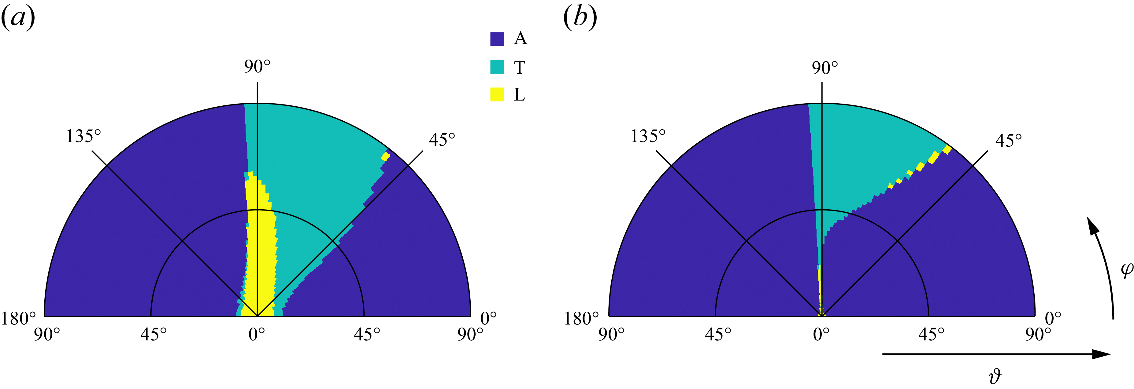
Phase diagrams of spheroid stable rotations with Stokes numbers
 $\widetilde {St_r}$
equal to (a) 0, (b) 0.1, (c) 1 and (d) 5, respectively. Here ‘A’, ‘T’ and ‘L’ represent the aligning, tumbling and logrolling modes, respectively. Black lines denote contours where the corresponding maximum eigenvalue is zero, indicating the neutral stability. The green and magenta lines separate distinct equilibrium-mode regimes. The colour-filled areas indicate the corresponding stable equilibrium modes. The abbreviations are as follows: A, aligning; L, logrolling; T, tumbling.

Figure 10 indicates the complexity of stable rotation modes of spheroids at different
 $\widetilde {St_r}$
. This is because of the competition between the fluid-inertial effect and the particle inertia. Here, the combinations of characters in different parameter regions represent the possible stable rotation modes of the spheroids, e.g. TL represents the rotation modes in which the spheroids have tumbling or logrolling stable modes. Note that the multistable rotation modes represent there is more than one stable equilibrium rotation modes for certain parameters. This indicates that, with different initial conditions, the rotation of a spheroid may converge to different stable rotation modes. At
 $\widetilde {St_r}=0$
in figure 10(a), inertia-free spheroids only have monostable modes. As is well known, when
 $\zeta =0$
, i.e. in the absence of fluid-inertial torque, spheroids follow Jeffery orbits. For
 $\zeta \gt 0$
, logrolling mode is stable for prolate spheroids, while aligning and tumbling modes separated by
 $\varLambda ^2+M^2=1$
are stable for oblate spheroids. These results are consistent with our previous study (Cui et al. Reference Cui, Liu, Qiu and Zhao2024). In figure 10(b), where
 $\widetilde {St_r}=0.1$
, satisfying
 $\widetilde {St_r}\ll 1$
, we observe that prolate spheroids have tumbling, TL and logrolling stable modes as
 $\zeta$
increases, while oblate spheroids with moderate aspect ratios have logrolling, TL, tumbling and aligning stable modes as
 $\zeta$
increases. For
 $\lambda \lesssim 0.05$
, there is an aligning–logrolling (AL) bistable mode between the regions of aligning and TL modes. Meanwhile, the region of the TL mode of prolate spheroids is much narrower than that of oblate ones, indicating that the condition of the TL mode for the prolate spheroids is more rigorous.
As particle inertia increases (see figure 10
c,d), the phase diagram for different stable rotation modes becomes more complicated. Regarding the oblate spheroids, the tristable ATL and bistable AT regions emerge and are enlarged as Stokes number increases, especially for the oblate spheroids with small aspect ratios. Meanwhile, the boundaries between logrolling and TL regions are prominently moved towards larger
 $\zeta$
and intersect with magenta lines
 $\varLambda ^2+M^2=1$
. For prolate spheroids, the TL region is significantly enlarged compared with that at
 $\widetilde {St_r}=0.1$
. According to figure 10, it is pronounced that inertial prolate spheroids experience tumbling, TL, and logrolling stable modes as
 $\zeta$
increases. Nevertheless, the parameter space of the TL region is significantly enlarged as Stokes number
 $\widetilde {St_r}$
increases.
In summary, when the fluid-inertial torque is considered, it is common to find multistable rotation modes of spheroids. These phenomena are mainly observed for oblate spheroids with large fluid inertia, while prolate spheroids only have a bistable TL region. Moreover, as particle inertia increases, the TL region of prolate spheroids is significantly enlarged and overwhelms that of oblate ones. This phase diagram indicates that when the fluid-inertial torque is taken into consideration, the rotations of oblate spheroids are more sensitive to the initial values, and exhibit variety compared with prolate spheroids.
4. Stability analysis versus simulation results
The stability analysis presented in this study is based on the governing equations of the PP model, which incorporates both the Jeffery torque (Jeffery Reference Jeffery1922) and the slip-induced fluid-inertial torque (Dabade et al. Reference Dabade, Marath and Subramanian2015). As such, the applicability of the present analysis is confined to specific regimes. First, the particle-to-fluid density ratio must be sufficiently large to neglect fluid inertia associated with the added mass. Second, the particle Reynolds number
 ${\textit{Re}}_{\!p}$
and the shear Reynolds number
 ${\textit{Re}}_\kappa$
must both satisfy
 ${\textit{Re}}_{\!p}, {\textit{Re}}_\kappa \ll 1$
to ensure the validity of the Jeffery and fluid-inertial torque models. Third, the slip-induced fluid-inertial torque derived by Dabade et al. (Reference Dabade, Marath and Subramanian2015) assumes a uniform ambient flow and is valid in the regime
 $\sqrt {{\textit{Re}}_\kappa } \ll {\textit{Re}}_{\!p} \ll 1$
. However, when the parameter
 $\zeta \equiv {\textit{Re}}_{\!p}/\sqrt {{\textit{Re}}_\kappa } \lt 1$
, the Jeffery torque becomes dominant. In this case, the leading-order shear-induced fluid-inertial torque, which scales with
 $\sqrt {{\textit{Re}}_\kappa }$
, vanishes due to the axisymmetric geometry of the spheroid (Candelier et al. Reference Candelier, Mehlig and Magnaudet2019). Furthermore, the next-order shear-induced torque, which scales with
 ${\textit{Re}}_\kappa$
, can also be neglected when
 ${\textit{Re}}_\kappa \ll \zeta ^2$
(see § 2.2). Therefore, the stability predictions shown in figure 10 remain valid even for cases with
 ${\textit{Re}}_{\!p} \lt \sqrt {{\textit{Re}}_\kappa }$
, provided that the condition
 ${\textit{Re}}_\kappa \ll \zeta ^2\ll 1$
is satisfied.
However, it is difficult to simultaneously satisfy all of the above conditions in practical situations. To further assess the validity of the stability analysis at finite Reynolds numbers, we conduct a series of numerical simulations about spheroids rotating in linear shear flows by using both PR and PP methods in this section. The parameters corresponding to representative stable rotational modes are listed in table 2. Details of the PR method employed in this study are provided in Appendix D. In all cases listed in table 2, the initial angular velocities are set to zero.
Settings of numerical simulations of spheroids in simple shear flows.
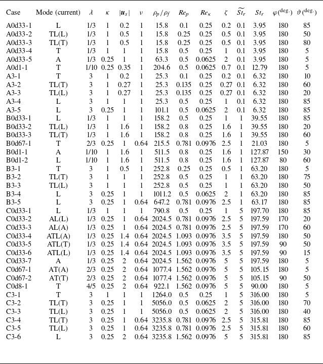
As shown in table 2, due to limitations of the current simulation methodology, not all cases fully satisfy the conditions required for the validity of the underlying model assumptions. These exceptions will be explicitly noted in the discussion of the corresponding cases. The trajectories of these cases in physical space for both PR and PP simulations are shown in figures 11–13. These figures serve to validate the predictions of our stability analysis based on the current slip-induced fluid-inertial torque model. It is important to note that the focus of this section is on assessing the stability of equilibrium rotational modes, rather than examining the detailed evolution of the spheroid orientation.
Trajectories of the endpoints for the symmetry axes of (b) oblate and (d) prolate spheroids rotating in shear flow with
 $\widetilde {St_r}=0.1$
. Red points in (a) and (c) are the corresponding particle parameters used in (b) and (d) for oblate and prolate spheroids, respectively. In (b) and (d), black lines are obtained by PP-DNS and red lines are computed by PR-DNS. Here, blue points represent the initial orientations of spheroids.

Trajectories of the endpoints for the symmetry axes of (b) oblate and (d) prolate spheroids rotating in shear flow with
 $\widetilde {St_r}=1$
. Red points in (a) and (c) are the corresponding particle parameters used in (b) and (d) for oblate and prolate spheroids, respectively. In (b) and (d), black lines are obtained by PP-DNS and red lines are computed by PR-DNS. Here, blue points represent the initial orientations of spheroids.

Trajectories of the endpoints for the symmetry axes of (b) oblate and (d) prolate spheroids rotating in shear flow with
 $\widetilde {St_r}=5$
. Red points in (a) and (c) are the corresponding particle parameters used in (b) and (d) for oblate and prolate spheroids, respectively. In (b) and (d), black lines are obtained by PP-DNS and red lines are computed by PR-DNS. Here, blue points represent the initial orientations of spheroids.

Regarding the results for
 $\widetilde {St_r} = 0.1$
, as shown in figure 11, the stability predictions obtained either by solving (2.11) or by using the PR method are consistent with the observed stable rotational modes. This agreement is particularly evident in the cases with large
 $\zeta$
, where the slip-induced fluid-inertial torque dominates the rotational dynamics. Since
 $\widetilde {St_r}$
is much smaller than unity, both the fluid-inertial torque and particle inertia are weak when
 $\zeta \lt 1$
. In this regime, subtle rotational tendencies of spheroids towards different stable modes arise depending on their initial orientations, particularly in the TL region of figure 11, which is consistent with the predictions from the stability analysis. When
 $\zeta = 1$
and
 $2$
, the trajectories of the endpoints of the spheroid symmetry axes show distinct behaviours: for oblate spheroids, the trajectories move away from the vortex axis, while for prolate spheroids, they move towards it. These observations are in agreement with the stability analysis. Furthermore, the trajectories computed using the PP method based on (2.11) show a good agreement with those obtained from the PR simulations. Nevertheless, for the PR simulations, the Reynolds number cannot be made arbitrarily small due to computational limitations. As a result, the density ratio is not sufficiently large, which may lead to potential deviations compared with the PP simulations, as observed in cases A0d33-1, A0d33-2 and A0d33-3. Moreover, for the oblate spheroid with
 $\lambda = 1/10$
and
 $\zeta = 0.7$
, the stable rotation mode is tumbling. Although the trajectories obtained from the PP and PR simulations exhibit notable deviations, they follow the same overall trend. This discrepancy may stem from an insufficiently large particle-to-fluid density ratio, based on the theory proposed by Einarsson et al. (Reference Einarsson, Candelier, Lundell, Angilella and Mehlig2015a
), provided that the theory for neutrally buoyant spheroids remains valid at large density ratios.
Figure 12 shows the trajectories of the symmetry axis endpoints of spheroids at
 $\widetilde {St_r}=1$
, where the effect of particle inertia becomes visible. Compared with the results at
 $\widetilde {St_r}=0.1$
, the competition between fluid inertia and particle inertia becomes fierce, leading to multiple stable rotation modes of spheroids, including bistable and tristable modes. From figure 12, although the parameter regimes for stable rotational modes become more complex, particularly for oblate spheroids, the stability analysis still provides accurate predictions when compared with both PP and PR simulation results. It is important to note that, due to limitations of the numerical methodology in the PR simulations, the particle Reynolds number
 ${\textit{Re}}_{\!p}$
approaches unity in cases with large
 $\zeta$
, making it difficult to strictly satisfy the condition
 ${\textit{Re}}_{\!p} \ll 1$
. As a result, small discrepancies appear in the endpoint trajectories between the PP and PR simulations. Nevertheless, figure 12 shows that these trajectory differences have minimal influence on the final stable rotational modes predicted by the stability analysis.
Compared with the results at
 $\widetilde {St_r} = 0.1$
and
 $\widetilde {St_r} = 1$
, the influence of particle inertia becomes more pronounced, as evidenced by the results shown in figure 13. As particle inertia increases, a larger slip-induced fluid-inertial torque is required to compete with particle inertia, leading to the different regimes with different multiple stable rotation modes. Meanwhile, with large Stokes numbers, the trajectories display distinct behaviours compared with those at smaller Stokes numbers. Notable examples include self-intersecting trajectories, as observed in cases C0d33-2 and C0d33-6, and spiral-in patterns towards the steady aligning mode, as seen in cases C0d33-3, C0d33-4, C0d33-7 and C0d67-1. It is important to note that the self-intersections only occur in the projected physical space. At the apparent intersection points, the angular velocities of the spheroid are different. Therefore, in the full six-dimensional phase space, which includes angular velocities, such self-intersections do not exist. Moreover, due to the limitations of numerical simulations, the PR cases at large
 $\widetilde {St_r}$
and large
 $\zeta$
do not strictly satisfy the assumptions underlying the torque model. As a result, notable differences arise between the PP and PR results. For example, in the case with
 $\zeta = 5$
, the maximum particle Reynolds number reaches 1.56, which may lead to deviations in the fluid-inertial torques between PP and PR methods. Nevertheless, this discrepancy has a minimal impact on the final stable rotation modes between these two methods. This limited influence can be illustrated by the ATL tristable regime, in which aligning, tumbling and logrolling modes coexist as stable rotation modes, depending on the initial orientation and angular velocity of the spheroid. The initial conditions define distinct attraction basins associated with each different rotation mode. If a given initial condition (not shown here) lies near the boundary between different attraction basins, the PP and PR simulations may evolve towards different stable modes due to the finite Reynolds number effects presented in the PR method. For instance, the PP simulation may predict convergence to an aligning mode with the particle’s symmetry axis fixed in space, whereas the PR simulation may result in continuous tumbling within the flow-gradient plane. These discrepancies, primarily induced by finite Reynolds number effects, manifest as blurred or diffuse basin boundaries in the PR simulations.
To further explore the effect of initial conditions, we present the attraction basins for different stable modes at multistable regimes under some specific parameters by means of the PP simulations, as shown in figures 14 and 15. In figure 14, we vary the initial orientations while keeping the initial angular velocity zero. To prevent the spheroid from being initialized precisely in an equilibrium orientation, a small perturbation is introduced into the initial conditions. From figure 14, the attraction basins corresponding to different stable equilibrium modes are clearly illustrated, indicating the dependency of the final state on
 $\widetilde {St_r}, \lambda$
and
 $\zeta$
. In figure 14(a,b), corresponding to weak particle and fluid inertia, the attraction zones appear and are symmetric about
 $\varphi =90^\circ$
. When
 $\widetilde {St_r}=1$
and
 $\zeta \geqslant 1$
, the logrolling attraction zone of a prolate spheroid becomes inclined (see figure 14
c), and the symmetry about
 $\varphi =90^\circ$
is broken for the oblate spheroid as shown in figure 14(d). Comparing figures 14(e) and 14(f), the logrolling attraction zone for prolate spheroids expands with increasing
 $\zeta$
. In figure 14(g,h), variations in
 $\zeta$
significantly alter the attraction basins in the initial orientation space. Figures 14(h) and 14(i) exhibit similar features, except for the disappearance of the logrolling attraction basin in figure 14(i).
Attraction basins in the initial orientation space (
 $\varphi$
,
 $\vartheta$
) are shown with zero initial angular velocities for multistable cases.

Attraction basins in the initial orientation space (
 $\varphi$
,
 $\vartheta$
) are shown for two different initial angular velocities in the case
 $\widetilde {St_r}=5, \lambda =1/3$
and
 $\zeta =3.5$
. The initial angular velocities are specified in the particle coordinate with
 $\omega _x^{\prime}=\omega _y^{\prime}=0$
and (a)
 $\omega _z^{\prime}=-0.2$
or (b)
 $\omega _z^{\prime}=0.2$
.

Regarding the impact of initial angular velocity, we present only one representative case
 $\widetilde {St_r}=5$
,
 $\lambda =1/3$
and
 $\zeta = 3.5$
in figure 15, as an example. Note that exploring the full range of angular velocity variations, which would involve the analysis in a six-dimensional phase space, is unrealistic in the current study. In figure 15, we examine the influence of initial angular velocity along the symmetry axis of spheroid
 $\omega _z^{\prime}$
. Specifically, we compare two cases with the same magnitude but opposite signs of
 $\omega _z^{\prime}$
. It is evident from figure 15 that the initial angular velocity has an appreciable change in the attraction basins. Compared with figure 14(h) with the same parameters but zero initial angular velocity, the logrolling attraction zone expands when setting
 $\omega _z^{\prime}=-0.2$
, whereas it contracts with
 $\omega _z^{\prime}=0.2$
.
5. Concluding remarks
In this study, we investigate the rotation of the inertial spheroids in shear flow with a non-negligible slip velocity at small Reynolds numbers, and we analyse the equilibrium rotation modes by a linear stability analysis. The results reveal intricate stable rotational behaviours of spheroids depending on various initial conditions and parameters of flow or particle, which can be predicted by our linear stability analysis even for the PR simulation with finite Reynolds numbers near
 $O(1)$
. The phase diagrams of the stable rotation modes of spheroids with three typical Stokes numbers
 $\widetilde {St_r}=0$
, 0.1, 1 and
 $5$
provide an overview of particle rotations in shear flow with a pronounced slip velocity. The key findings are concluded as follows.
Different from the earlier works that neglected slip-induced fluid-inertial torque (Lundell & Carlsson Reference Lundell and Carlsson2010; Challabotla et al. Reference Challabotla, Nilsen and Andersson2015), we find bistable and tristable behaviours of spheroids in shear flow with
 ${\textit{Re}}_{\!p}, {\textit{Re}}_\kappa \ll 1$
. According to the phase diagrams of the spheroid motions, the stable rotation varies with the particle shape, fluid inertia and particle inertia, indicating a fierce competition of the effects between particle inertia and fluid inertia. When the effect of fluid-inertial torque is weaker than that of particle inertia, oblate spheroids tend to logroll and prolate spheroids tend to tumble in the flow-gradient plane, which is consistent with the results reported in the previous studies in the absence of fluid-inertial torque (Lundell & Carlsson Reference Lundell and Carlsson2010; Challabotla et al. Reference Challabotla, Nilsen and Andersson2015). Regardless of particle inertia, as fluid-inertial torque increases, the stable rotation modes of prolate spheroids gradually experience tumbling, TL and logrolling regions. Notably, the critical threshold
 $\zeta _c$
separating these regimes increases with the Stokes number, approximately following the scaling
 $\zeta _c^2 \propto \widetilde {St_r}$
. Meanwhile, the TL region becomes pronounced and its parameter space is enlarged as the particle increases, reflecting that the corresponding fluid inertia to balance the particle inertial effect should be larger. Regarding oblate spheroids, the rotation modes are much more complex than those of prolate ones as particle inertia increases. For the oblate spheroid with weak particle inertia, as fluid-inertial torque increases, the stable modes with moderate aspect ratios experience logrolling, TL and tumbling regions, while the extremely flat oblate spheroids may experience additional AL and aligning regions. That is because the fluid-inertial torque acting on the extremely flat oblate spheroids is more pronounced. The oblate spheroids with large particle inertia have additional ATL and AT mode regions, where particles have multistable rotation motions, as the fluid inertia increases. Nevertheless, the corresponding areas of the TL and tumbling regions of oblate spheroids are gradually less than those of prolate ones as particle inertia increases.
Furthermore, the comparisons between the stability analysis results and the spheroids rotations by PP and PR simulations demonstrate the predicted stable rotation modes by the stability analysis are valid even when
 $\sqrt {{\textit{Re}}_\kappa }\ll {\textit{Re}}_{\!p}\ll 1$
is not strictly upheld. Although the PP results have observed differences in the rotation processes from the PR results with Reynolds numbers over
 $O(1)$
, the final stable rotation modes of PP and PR simulations with the same settings are still consistent. This further supports the validity of the torque model that combines the slip-induced fluid-inertial torque (Dabade et al. Reference Dabade, Marath and Subramanian2015) with the viscous Jeffery torque (Jeffery Reference Jeffery1922) for spheroidal particles in strong-shear environments.
In the present study, we focus on the stability for equilibrium rotations of spheroids in steady shear flows with a streamwise slip velocity. Here, the slip velocity is an artificial parameter because the translational motion is constrained. The potential occurrence of trajectory self-intersections during the evolution of the particle orientation from an arbitrary initial condition to the final state is beyond the scope of the current work. Nevertheless, the issues related to trajectory self-intersections and the nonlinear dynamics of particle motion are indeed intriguing and merit further investigation in future work. In reality, however, the slip velocity is dynamic, varying with the particle motion and influenced by the particle inertia. Therefore, it is valuable to investigate the coupling between translational and rotational dynamics of spheroids in shear flows in the future, such as the settling of spheroids in vertical shear flows. Moreover, since unsteady flows are prevalent in practical applications, exploring the effect of flow unsteadiness, such as flow fluctuations, on spheroid motion constitutes another interesting direction for future works.
Acknowledgements
The authors are grateful to the anonymous referees for their constructive comments and suggestions.
Funding
This work was supported by the Natural Science Foundation of China (grant numbers 12302285, 12388101, 12472224 and 92252104), the Fundamental Research Funds for the Central Universities and the China Postdoctoral Science Foundation (grant number 2022M721849).
Declaration of interests
The authors report no conflict of interest.
Data availability statement
The data of PP and PR simulations for a single spheroid are available at https://github.com/Cui-ZW/PP-PRData-Spheroids.
Appendix A. Expression of
$\boldsymbol{F}_{\boldsymbol{\lambda}}$

For the prolate spheroids (
 $\lambda \gt 1$
), the eccentricity of spheroid
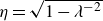 $\eta =\sqrt {1-\lambda ^{-2}}$
and the shape function
 $F_\lambda$
is expressed as (Dabade et al. Reference Dabade, Marath and Subramanian2015)
 \begin{align} F_\lambda &=\frac {-\pi \eta ^2\left(420\eta +2240\eta ^3+4249\eta ^5-2152\eta ^7\right)}{315\left[\left(\eta ^2+1\right)\tanh ^{-1}\eta -\eta \right]^2\left[\left(1-3\eta ^2\right)\tanh ^{-1}\eta -\eta \right]}\nonumber\\ &\quad +\frac {\pi \eta ^2\left(420+3360\eta ^2+1890\eta ^4-1470\eta ^6\right)\tanh ^{-1}\eta }{315\left[\left(\eta ^2+1\right)\tanh ^{-1}\eta -\eta \right]^2\left[\left(1-3\eta ^2\right)\tanh ^{-1}\eta -\eta \right]}\nonumber\\ &\quad -\frac {\pi \eta ^2\left(1260\eta -1995\eta ^3+2730\eta ^5-1995\eta ^7\right)\left(\tanh ^{-1}\eta \right)^2}{315\left[\left(\eta ^2+1\right)\tanh ^{-1}\eta -\eta \right]^2\left[\left(1-3\eta ^2\right)\tanh ^{-1}\eta -\eta \right]}. \end{align}
Regarding the oblate spheroids (
 $0\lt \lambda \lt 1$
), the eccentricity of spheroid is
 $\eta =\sqrt {1-\lambda ^2}$
and the corresponding shape function is (Dabade et al. Reference Dabade, Marath and Subramanian2015)
 \begin{align} F_\lambda &=\frac {\pi \eta ^3\left(-420+3500\eta ^2-9989\eta ^4+4757\eta ^6\right)}{315\left[-\eta \sqrt {1-\eta ^2}+\left(1+2\eta ^2\right)\arcsin \eta \right]\left[\eta \sqrt {1-\eta ^2}+\left(2\eta ^2-1\right)\arcsin \eta \right]^2}\nonumber \\ &\quad+\frac {210\pi \eta ^2\left(2-24\eta ^2+69\eta ^4-67\eta ^6+20\eta ^8\right)\arcsin \eta }{315\sqrt {1-\eta ^2}\!\left[\!-\eta \sqrt {1-\eta ^2}+\left(1+2\eta ^2\right)\arcsin \eta \!\right]\!\left[\!\eta \sqrt {1-\eta ^2}+\left(2\eta ^2-1\right)\arcsin \eta \!\right]^2}\nonumber \\ &\quad+\frac {105\pi \eta ^3\left(12-17\eta ^2+24\eta ^4\right)\left(\arcsin \eta \right)^2}{315\left[-\eta \sqrt {1-\eta ^2}+\left(1+2\eta ^2\right)\arcsin \eta \right]\left[\eta \sqrt {1-\eta ^2}+\left(2\eta ^2-1\right)\arcsin \eta \right]^2}. \end{align}
Appendix B. Expansion for the angular dynamics of spheroidal particles at small Stokes number
We assume that for small Stokes number
 $St_r$
the angular velocity of the particle is almost the same as
 \begin{equation} \boldsymbol \omega =\boldsymbol \omega _0+St_r \boldsymbol \omega _1+O\big(St_r^2\big). \end{equation}
By inserting (B1) into (2.11), we can obtain
 \begin{align} St_r \unicode{x1D63E}\boldsymbol{\cdot }\frac {\mathrm{d}{\boldsymbol \omega _0}}{\mathrm{d}t}+\ldots &=\boldsymbol \varOmega -\boldsymbol \omega _0-St_r \boldsymbol \omega _1+\boldsymbol n\times (\varLambda \unicode{x1D64E}+M\hat {\boldsymbol u}_s\hat {\boldsymbol u}_s)\boldsymbol{\cdot }\boldsymbol n \nonumber\\&\quad-\boldsymbol n\times (St_r C_\perp \varLambda \boldsymbol \omega _0 \boldsymbol \omega _0)\boldsymbol{\cdot }\boldsymbol n+\ldots . \end{align}
Then, matching the term by order in
 $St_r$
, the
 $O(1)$
term is
 \begin{equation} \boldsymbol \omega _0=\boldsymbol \varOmega +\boldsymbol n\times (\varLambda \unicode{x1D64E}+M\hat {\boldsymbol u}_s\hat {\boldsymbol u}_s)\boldsymbol{\cdot }\boldsymbol n, \end{equation}
and
 $O(St_r)$
term satisfies
 \begin{equation} \boldsymbol \omega _1=-\unicode{x1D63E}\boldsymbol{\cdot }\frac {\mathrm{d}{\boldsymbol \omega _0}}{\mathrm{d}t}-\boldsymbol n\times ( C_\perp \varLambda \boldsymbol \omega _0 \boldsymbol \omega _0)\boldsymbol{\cdot }\boldsymbol n. \end{equation}
If we only consider one-order expansion, the corresponding orientational dynamics of a spheroid is
 \begin{equation} \frac {\mathrm{d}{\boldsymbol n}}{\mathrm{d}t}=\boldsymbol \omega \times \boldsymbol n=\boldsymbol \omega _0\times \boldsymbol n+St_r \boldsymbol \omega _1 \times \boldsymbol n. \end{equation}
We continue to find the first derivative of (B3) along the time
 $t$
, and the term of
 ${\mathrm{d}{\boldsymbol \omega _0}}/{\mathrm{d}t}$
is
 \begin{align} \frac {\mathrm{d}{\boldsymbol \omega _0}}{\mathrm{d}t}&=\frac {\mathrm{d}{\boldsymbol n}}{\mathrm{d}t}\times (\varLambda \unicode{x1D64E}+M\hat {\boldsymbol u}_s\hat {\boldsymbol u}_s)\boldsymbol{\cdot }\boldsymbol n+\boldsymbol n\times (\varLambda \unicode{x1D64E}+M\hat {\boldsymbol u}_s\hat {\boldsymbol u}_s)\boldsymbol{\cdot }\frac {\mathrm{d}{\boldsymbol n}}{\mathrm{d}t} \nonumber\\ &=\unicode{x1D64A}\boldsymbol{\cdot }\boldsymbol n\times \unicode{x1D63D}_s\boldsymbol{\cdot }\boldsymbol n+\boldsymbol n\times (\unicode{x1D63D}_s\boldsymbol{\cdot }\unicode{x1D64A}+\unicode{x1D63D}_s\boldsymbol{\cdot }\unicode{x1D63D}_s-2(\unicode{x1D63D}_s:\boldsymbol n \boldsymbol n)\unicode{x1D63D}_s)\boldsymbol{\cdot }\boldsymbol n. \end{align}
Here,
 $\unicode{x1D63D}_s=\varLambda \unicode{x1D64E}+M\hat {\boldsymbol u}_s\hat {\boldsymbol u}_s$
, which is a symmetric matrix. For simplicity, we use
 $\unicode{x1D63D}_s$
hereinafter. Inserting (B6) into (B4), we find
 \begin{align} \boldsymbol \omega _1&=-\unicode{x1D63E} \boldsymbol{\cdot }(\unicode{x1D64A}\boldsymbol{\cdot }\boldsymbol n\times \unicode{x1D63D}_s\boldsymbol{\cdot }\boldsymbol n)\nonumber \\ &\quad+C_\perp \boldsymbol n \times \left(-\unicode{x1D63D}_s\boldsymbol{\cdot }\unicode{x1D64A}-\unicode{x1D63D}_s \boldsymbol{\cdot }\unicode{x1D63D}_s+2\left(\unicode{x1D63D}_s:\boldsymbol n \boldsymbol n\right)\unicode{x1D63D}_s-\varLambda \boldsymbol \omega _0 \boldsymbol \omega _0\right)\boldsymbol{\cdot }\boldsymbol n .\end{align}
Next, inserting (B3) and (B7) into (B5), we get
 \begin{equation} \frac {\mathrm{d}{\boldsymbol n}}{\mathrm{d}t}=\unicode{x1D64A}\boldsymbol{\cdot }\boldsymbol n+\unicode{x1D63D}_s\boldsymbol{\cdot }\boldsymbol n-(\unicode{x1D63D}_s:\boldsymbol n \boldsymbol n)\boldsymbol n+StC_\perp [(\unicode{x1D63D}_s:\boldsymbol n\boldsymbol n) \unicode{x1D64A} \boldsymbol{\cdot }\boldsymbol n+\unicode{x1D640}_s\boldsymbol{\cdot }\boldsymbol n-(\unicode{x1D640}_s :\boldsymbol n\boldsymbol n) \boldsymbol n], \end{equation}
where
 $\unicode{x1D640}_s=-\unicode{x1D63D}_s\boldsymbol{\cdot }\unicode{x1D64A}-\unicode{x1D63D}_s \boldsymbol{\cdot }\unicode{x1D63D}_s+2(\unicode{x1D63D}_s:\boldsymbol n \boldsymbol n)\unicode{x1D63D}_s-\varLambda \boldsymbol \omega _0 \boldsymbol \omega _0$
. Meanwhile, the term link to
 $\boldsymbol \omega _0 \boldsymbol \omega _0$
can be expressed as
 \begin{align} \varLambda \boldsymbol \omega _0\boldsymbol \omega _0\boldsymbol{\cdot }\boldsymbol n-\varLambda (\boldsymbol n\boldsymbol{\cdot }\boldsymbol \omega _0\boldsymbol \omega _0\boldsymbol{\cdot }\boldsymbol n )\boldsymbol n &=\varLambda (\boldsymbol \varOmega +\boldsymbol n\times \unicode{x1D63D}_s\boldsymbol{\cdot }\boldsymbol n)(\boldsymbol \varOmega +\boldsymbol n\times \unicode{x1D63D}_s\boldsymbol{\cdot }\boldsymbol n)\boldsymbol{\cdot }\boldsymbol n\nonumber \\ &\quad-\varLambda \boldsymbol n\boldsymbol{\cdot }(\boldsymbol \varOmega +\boldsymbol n\times \unicode{x1D63D}_s\boldsymbol{\cdot }\boldsymbol n)(\boldsymbol \varOmega +\boldsymbol n\times \unicode{x1D63D}_s\boldsymbol{\cdot }\boldsymbol n)\boldsymbol{\cdot }\boldsymbol n\boldsymbol n\nonumber \\ &=\varLambda \boldsymbol \varOmega \boldsymbol \varOmega \boldsymbol{\cdot }\boldsymbol n+\varLambda (\boldsymbol n\times \unicode{x1D63D}_s\boldsymbol{\cdot }\boldsymbol n)\boldsymbol \varOmega \boldsymbol{\cdot }\boldsymbol n-\varLambda (\boldsymbol \varOmega \boldsymbol{\cdot }\boldsymbol n)(\boldsymbol \varOmega \boldsymbol{\cdot }\boldsymbol n)\boldsymbol n\nonumber \\ &=\varLambda [\boldsymbol \varOmega \boldsymbol \varOmega \boldsymbol{\cdot }\boldsymbol n-(\boldsymbol \varOmega \boldsymbol{\cdot }\boldsymbol n)(\boldsymbol \varOmega \boldsymbol{\cdot }\boldsymbol n)\boldsymbol n]+\varLambda (\boldsymbol n\times \unicode{x1D63D}_s\boldsymbol{\cdot }\boldsymbol n)\boldsymbol \varOmega \boldsymbol{\cdot }\boldsymbol n. \end{align}
Here,
 $\boldsymbol \varOmega$
is fluid rotation and satisfies
 $\boldsymbol \varOmega =-({1}/{2}) \epsilon :\unicode{x1D64A}$
with rotation tensor
 $\unicode{x1D64A}$
. Therefore, (B9) can also be expressed as
 \begin{align} \varLambda \boldsymbol \omega _0\boldsymbol \omega _0\boldsymbol{\cdot }\boldsymbol n-\varLambda (\boldsymbol n\boldsymbol{\cdot }\boldsymbol \omega _0\boldsymbol \omega _0\boldsymbol{\cdot }\boldsymbol n )\boldsymbol n &=\varLambda [\unicode{x1D64A}\boldsymbol{\cdot }\unicode{x1D64A}+\unicode{x1D64A} \boldsymbol{\cdot }\unicode{x1D63D}_s-(\unicode{x1D63D}_s:\boldsymbol n\boldsymbol n)\unicode{x1D64A}]\boldsymbol{\cdot }\boldsymbol n\nonumber\\ &\quad -\varLambda \boldsymbol n\boldsymbol{\cdot }(\unicode{x1D64A}\boldsymbol{\cdot }\unicode{x1D64A}+\unicode{x1D64A}\boldsymbol{\cdot }\unicode{x1D63D}_s)\boldsymbol{\cdot }\boldsymbol n\boldsymbol n. \end{align}
The final form of the orientational dynamics of a spheroid is
 \begin{align} \frac {\mathrm{d}{\boldsymbol n}}{\mathrm{d}t}&=\unicode{x1D64A}\boldsymbol{\cdot }\boldsymbol n+\unicode{x1D63D}_s\boldsymbol{\cdot }\boldsymbol n-(\unicode{x1D63D}_s:\boldsymbol n \boldsymbol n)\boldsymbol n+StC_\perp \lbrace (\unicode{x1D63D}_s:\boldsymbol n\boldsymbol n) \unicode{x1D64A} \boldsymbol{\cdot }\boldsymbol n\nonumber \\ &\quad+[-\unicode{x1D63D}_s\boldsymbol{\cdot }\unicode{x1D64A}-\unicode{x1D63D}_s \boldsymbol{\cdot }\unicode{x1D63D}_s+2(\unicode{x1D63D}_s:\boldsymbol n \boldsymbol n)\unicode{x1D63D}_s]\boldsymbol{\cdot }\boldsymbol n-\boldsymbol n\boldsymbol{\cdot }[-\unicode{x1D63D}_s\boldsymbol{\cdot }\unicode{x1D64A}-\unicode{x1D63D}_s \boldsymbol{\cdot }\unicode{x1D63D}_s\nonumber \\ &\quad+2(\unicode{x1D63D}_s:\boldsymbol n \boldsymbol n)\unicode{x1D63D}_s] \boldsymbol{\cdot }\boldsymbol n\boldsymbol n -\varLambda [\unicode{x1D64A}\boldsymbol{\cdot }\unicode{x1D64A}+\unicode{x1D64A} \boldsymbol{\cdot }\unicode{x1D63D}_s-(\unicode{x1D63D}_s:\boldsymbol n\boldsymbol n)\unicode{x1D64A}]\boldsymbol{\cdot }\boldsymbol n\nonumber \\ &\quad+\varLambda \boldsymbol n\boldsymbol{\cdot }(\unicode{x1D64A}\boldsymbol{\cdot }\unicode{x1D64A}+\unicode{x1D64A}\boldsymbol{\cdot }\unicode{x1D63D}_s)\boldsymbol{\cdot }\boldsymbol n\boldsymbol n\rbrace . \end{align}
The comparison of the results computed by the weakly inertial form (see (B11)) and the exact form (see (2.11)) is shown in figure 16, reflecting that when
 $\widetilde{{St}_r}\equiv StC_\perp$
is small, the weakly inertial form of orientational dynamics of spheroid can accurately capture the rotations.
Projecting endpoint trajectories of spheroids in shear flows computed by the weakly inertial form (blue lines, see (B11)) and exact form (red dashed lines, see (2.11)). (a,b) Prolate spheroids with aspect ratio
 $\lambda =5$
, fluid-inertial strength
 $\zeta =0.1$
and initial orientation
 $\boldsymbol n(0)=[0.0990,0.0990,0.9901]$
, where
 $\widetilde {St_r}=0.5$
in (a) and
 $\widetilde {St_r}=0.7$
in (b). (c,d) Oblate spheroids with
 $\lambda =1/5$
,
 $\zeta =0.1$
, and
 $\boldsymbol n(0)=[0.7053,0.7053,0.0705]$
, where
 $\widetilde {St_r}=0.1$
in (c) and
 $\widetilde {St_r}=0.25$
in (d). Note that the black circles are the initial orientations.

Appendix C. Method of discrete Floquet theory
Floquet theory is a method to analyse the stability of periodic motions (Joseph Reference Joseph1976; Chicone Reference Chicone2006). For any perturbation equation, the compact form is
 \begin{equation} \frac {\mathrm{d}{\delta \boldsymbol x(t)}}{\mathrm{d}t} = \unicode{x1D64C}(t) \boldsymbol{\cdot }\delta \boldsymbol x, \end{equation}
where
 $\delta \boldsymbol x$
is the perturbation, and
 $\unicode{x1D64C}$
is the stable matrix depending on time. The solution of this equation is
 \begin{equation} \delta \boldsymbol x(t_0+T_{\!p}) =\unicode{x1D652}_{t_0}^{\;t_0+T_{\!p}}\boldsymbol{\cdot }\delta \boldsymbol x(t_0), \end{equation}
where
 $T_{\!p}$
is the period, and
 $\unicode{x1D652}_{t_0}^{\;t_0+T_{\!p}}$
is the monodromy matrix reflecting a Poincaré map connecting two disturbances at
 $t_0$
and
 $t_0+T_{\!p}$
. For a more general form, the fundamental solution after a period is
 \begin{equation} \unicode{x1D655}(t+T_{\!p})= \unicode{x1D652}\boldsymbol{\cdot }\unicode{x1D655}(t), \end{equation}
where
 $\boldsymbol Z$
is the corresponding fundamental matrix of the solution (Joseph Reference Joseph1976; Chicone Reference Chicone2006), i.e.
 $\delta \boldsymbol x(t)=\unicode{x1D655}(t) \boldsymbol{\cdot }\delta \boldsymbol x(t_0)$
. In this section, it is essential to obtain
 $\unicode{x1D652}$
numerically. According to Varney & Green (Reference Varney and Green2017) and Cui et al. (Reference Cui, Zhao, Huang and Xu2019), to acquire
 $\unicode{x1D652}$
close to the true solution, we divide a periodic motion into many small pieces with
 $\Delta t =T_{\!p}/N$
, where
 $N$
is the number of the pieces. For each
 $\Delta t$
, the stable matrix
 $\unicode{x1D64C}$
is assumed as constant. Consequently, we can obtain the monodromy matrix in each interval, denoted as
 $\unicode{x1D64B}_i=\unicode{x1D652}_{t_i}^{\;t_i+\Delta t}$
, and the final
 $\unicode{x1D652}$
during a period can be obtained by multiplying all
 $\unicode{x1D64B}_i$
, that is
 \begin{align} \unicode{x1D655}_{i+1}&=\unicode{x1D64B}_i\boldsymbol{\cdot }\unicode{x1D655}_i=\unicode{x1D64B}_i\boldsymbol{\cdot }\unicode{x1D64B}_{i-1}\boldsymbol{\cdot }\unicode{x1D655}_{i-1}=\unicode{x1D64B}_i\boldsymbol{\cdot }\unicode{x1D64B}_{i-1}\ldots \unicode{x1D64B}_0\boldsymbol{\cdot }\unicode{x1D655}_{0}= \unicode{x1D652}\boldsymbol{\cdot }\unicode{x1D655}_0,\nonumber \\ \unicode{x1D652} &=\unicode{x1D64B}_i\boldsymbol{\cdot }\unicode{x1D64B}_{i-1}\ldots \unicode{x1D64B}_0,\nonumber \\ \unicode{x1D652}(0)&=\unicode{x1D640},\nonumber \\ \unicode{x1D652}(T)&=\unicode{x1D64B}_N\boldsymbol{\cdot }\unicode{x1D64B}_{N-1}\ldots \unicode{x1D64B}_0. \end{align}
Here,
 $\unicode{x1D640}$
is an identity matrix, subscript
 $0$
represents the beginning of a period, and each
 $\unicode{x1D64B}_i$
is obtained via fourth-order Runge–Kutta method as follows (Cui et al. Reference Cui, Zhao, Huang and Xu2019):
 \begin{align} \unicode{x1D64B}_i&=\unicode{x1D640}+\frac {1}{6}\Delta t(\unicode{x1D660}_1+2\unicode{x1D660}_2+2 \unicode{x1D660}_3+\unicode{x1D660}_4),\nonumber \\ \unicode{x1D660}_1&=\unicode{x1D64C}_t,\nonumber \\ \unicode{x1D660}_2&=\frac {1}{2}\unicode{x1D64C}_{t+1/2\Delta t}(2\unicode{x1D640}+\Delta t \unicode{x1D64C}_t),\nonumber \\ \unicode{x1D660}_3&=\frac {1}{4}\unicode{x1D64C}_{t+1/2\Delta t}(4\unicode{x1D640}+2\Delta t \unicode{x1D64C}_{t+1/2\Delta t}+\Delta t^2\unicode{x1D64C}_t \unicode{x1D64C}_{t+1/2\Delta t}),\nonumber \\ \unicode{x1D660}_4&=\frac {1}{4}\unicode{x1D64C}_{t+\Delta t}(4\unicode{x1D640}+4\Delta t \unicode{x1D64C}_{t+1/2\Delta t}+2\Delta t^2 \unicode{x1D64C}_{t+1/2\Delta t}^2+\Delta t^3\unicode{x1D64C}_{t}\unicode{x1D64C}_{t+1/2\Delta t}^2). \end{align}
Here,
 $i=0, 1 \ldots N-1$
and
 $t=i\Delta t$
. The eigenvalues
 $\varrho _i$
of
 $\unicode{x1D652}(T)$
are the Floquet multipliers, and their relationship with stable matrix
 $\unicode{x1D64C}$
satisfies
 \begin{equation} \det (W(T))= \varrho _1 \varrho _2 \ldots \varrho _n=\exp \left(\int _0^{T_{\!p}} \textit{Tr}(\unicode{x1D64C}(s)) {\rm d}s\right)\!. \end{equation}
The stability of the dynamic system is determined by the maximum of Floquet multipliers, i.e.
 $\varrho _m=|\varrho _i|_{max }$
. When
 $\varrho _m\lt 1$
, the system is linearly stable; when
 $\varrho _m\gt 1$
, the system is unstable; when
 $\varrho _m=1$
, the system is neutrally stable. In this study, we use the Floquet exponent
 $\gamma _m=\ln (\varrho _m)/T_{\!p}$
to plot the contour of the stability map.
Appendix D. Immersed boundary method for PR simulation
In this study, we employ a series of numerical simulations for a finite-size spheroid rotating in shear flows by immersed boundary method (Peskin Reference Peskin2002), to demonstrate the validity of the results predicted by stability analysis. The background fluid phase is governed by the Naiver–Stokes and continuity equations, i.e.
 \begin{align} \frac {\partial \boldsymbol{u}}{\partial t}+(\boldsymbol{u} \boldsymbol{\cdot }\boldsymbol{\nabla }) \boldsymbol{u}&=-\frac {1}{\rho _{\!f}} \boldsymbol{\nabla }\! p+\nu {\nabla} ^{2} \boldsymbol{u}+\boldsymbol{f}_{\!L}, \nonumber\\ \boldsymbol{\nabla } \boldsymbol{\cdot }\boldsymbol{u}&=0. \end{align}
Here,
 $\boldsymbol u$
is the fluid velocity,
 $\rho _f$
is the fluid density,
 $\nu$
is the kinematic viscosity and
 $\boldsymbol f_{\!L}$
is the force acting on fluid from the boundary of the particles. In this study, the face of the particle is discretized into uniform Lagrangian points, denoted as
 $\unicode{x1D653}_L$
, which follow the rotation of the particle. At each moment, the forces acting on the
 $\unicode{x1D653}_L$
are
 \begin{equation} \boldsymbol{F}_{\!L}=-C_\theta \left [\int _{0}^{t}\left (\boldsymbol{U}_{\! i b}-\boldsymbol{U}\right ) \mathrm{d} t+\Delta t\left (\boldsymbol{U}_{\! i b}-\boldsymbol{U}\right )\right ]\!, \end{equation}
where
 $C_\theta$
is the large penalty coefficient,
 $\Delta t$
is the time interval,
 $\boldsymbol U_{\!ib}$
represents the fluid velocity at
 $\unicode{x1D653}_{\!L}$
, which is interpolated from the velocities at surrounding grids
 $\unicode{x1D66D}_E$
, i.e.
 \begin{equation} \boldsymbol{U}_{\! i b}=\sum \boldsymbol{u} \delta _{h}(\boldsymbol{X}_{\!L}-\boldsymbol{x}_{\!E}) \Delta\! V. \end{equation}
Here,
 $\Delta\! V=h^3$
, where
 $h$
represents the length of gird cells along three directions. The smooth function
 $\delta _h$
for interpolating is expressed as
 \begin{equation} \delta _{h}(x)=\frac {1}{h^{3}} \phi \left (\frac {x}{h}\right ) \phi \left (\frac {y}{h}\right ) \phi \left (\frac {z}{h}\right )\!, \end{equation}
where
 $\phi$
is a four-points
 $\delta$
function (Peskin Reference Peskin2002), as follows:
 \begin{equation} \phi (r)= \begin{cases}\dfrac {1}{8}\left (3-2|r|+\sqrt {1+4|r|-4 r^{2}}\right )\!, & 0 \leqslant |r|\lt 1, \\[8pt] \dfrac {1}{8}\left (5-2|r|-\sqrt {-7+12|r|-4 r^{2}}\right )\!, & 1 \leqslant |r|\lt 2, \\ 0, & 2 \leqslant |r| .\end{cases} \end{equation}
Finally, the surface force exerting on the particle
 $\boldsymbol F_{\!L}$
is transferred to the Euler grid points through the
 $\delta _{h}$
function, that is
 \begin{equation} \boldsymbol{f}_{\!L}=\sum \boldsymbol{F}_{\!L} \delta _{h}(\boldsymbol{x}_{E}-\boldsymbol{X}_L) \Delta\! V. \end{equation}
In the current study, the centre of the spheroidal particle is set in the centreline between two parallel plates. By moving two plates with different velocities, we can obtain different shear flows with different shear rates and centre velocities, as shown in figure 17.
Schematic of spheroids rotating in shear flow driven by moving parallel plates.

We set the length of the major axis as a unit, namely
 $D=1$
, and the corresponding length of the semimajor axis
 $R$
is equal to
 $0.5$
. The computational domain sizes in streamwise, wall-normal and spanwise directions are
 $[-4D,4D]$
. By moving the upper and lower walls, a linear shear flow in the form
 $u=\kappa y+U_s$
is formed around the particle based on the velocity difference between the two walls. Where
 $u$
is the flow velocity,
 $\kappa$
is the shear rate,
 $y$
is the normal height position and
 $U_s$
is the slip velocity between the fluid and the particles. At the same time, we impose no-slip conditions on the upper and lower walls, and periodic boundary conditions in the span direction. Dirichlet boundary conditions (
 $u=\kappa y+U_s,v=0,w=0$
) are applied at the inlet, and convection boundary conditions are used at the outlet. In most cases, the flow grid resolution is 32 uniform grid points per unit length
 $D$
. For cases with an aspect ratio of
 $\lambda = 1/10$
, a finer resolution of 64 grid points per unit length
 $D$
is employed. Accordingly, the maximum total mesh size reaches
 $512^3 \approx 134\times 10^6$
.
The centre of the spheroidal particle is fixed at the centre position
 $(0,0,0)$
of the computational domain, but the rotational freedom of the particle is not restricted. In this article, the Reynolds number of particles is defined based on the particle semimajor axis, the corresponding particle Reynolds number is
 ${\textit{Re}}_{\!p}=U_sR/\nu$
, and the shear Reynolds number is
 ${\textit{Re}}_\kappa =\kappa R^2/\nu$
. In addition, since we only consider the rotational behaviour of the particle, its translational behaviour is limited, so we only define the rotational inertia
 $St_r=\rho _{\!p}/\rho _{\!f}{\textit{Re}}_\kappa$
of the particle. The external force on the particle is obtained by integrating the stress on the particle surface, and the external force is brought into the Euler equation of rigid body free rotation to solve (see 2.2). The relevant specific process of the method can be found in Li et al. (Reference Li, Cui, Huang, Zhao and Xu2018).