1. Introduction
Mapping is a prerequisite for robot path planning and task execution, which requires the robot to firstly explore the environment and complete the construction of the map. How to complete the exploration of the whole environment quickly and accurately has been the research focus of the majority of scholars. Among them, one of the mainstream methods is the frontier-based exploration method [Reference Yamauchi1], which divides the exploration space into known areas and unknown areas, and guides the robot to move to frontiers to complete the exploration of the unknown space. The extraction and selection of frontiers are one of the key issues for the frontier-based exploration method. A method of extracting frontiers using the Rapidly-exploring Random Tree (RRT) came into being, which generates the frontiers efficiently with less computing resource consumption [Reference Liu, Lv, Yuan, Chi, Chen and Sun2]. In the RRT method, an information gain model is constructed to distinguish revenue values of different frontiers and the frontier with the maximum value is selected as the target point to explore. Most of them assume that the sensor has a good perception effect on the surrounding environment and they usually focus on minimizing the number of accessible frontiers while ignoring the robot drift and the limitations of the perception. However, when the sensing range of the sensor is limited, the uncertainty of the trajectory increases, which may cause a great robot drift and even localization lost. In this case, how to balance the map information gain and the trajectory uncertainty is crucial for the motion decision of the robot in the process of robot exploration. In this article, we focus on the exploration and research of this kind of problem.
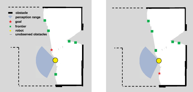
And we find when the environment is relatively empty and the distance to the nearest obstacle is beyond the perception range of the sensor, the robot can only obtain limited information and will wander near the current point, which causes the low efficiency of the exploration. This phenomenon often occurs in real-world applications, and we define this phenomenon as perceptual uncertainty. One reason is that the existing information gain model of frontier only takes into account the information gain and the path cost of the exploration process and neglects the perceptual uncertainty. A typical example is shown in Fig. 1. The figure shows an empty scene where the distance from the robot to the nearest obstacle exceeds the sensing range of the laser rangefinder. The target point selected in the left figure contains more unknown areas whereas with more perceptual uncertainty. However, the current environment structure is beyond the range of sensor perception, when the robot reaches the target point, it cannot effectively update the area where the frontiers are located, and the robot will linger in this empty area for a long time.
An illustration of a typical case with perceptual uncertainty. The red star represents the target frontiers selected by different decision-making methods. The left shows the target point obtained by considering the information gain and path cost, and the right shows the target point obtained by our method. Obviously, more obstacles are around the right target.

To solve the aforementioned problem, a decision-making method by integrating estimated path information gain with the current information gain model is proposed. In the process of frontier selection, the environmental information that a robot can obtain on its trajectory from the current pose to the candidate frontier is estimated, which is defined as the estimated path information gain. This idea is inspired by environmental information, such as obstacles that can assist the robot in localization. The more obstacles the robot encounters in the process of moving, the lower the uncertainty of localization and perception. When introducing the estimated path information gain in the decision process, a frontier with more abundant environmental information will be selected. As shown on the right of Fig. 1, the target points selected by our method in the right figure contain more environmental information. Exploring towards the frontiers with rich information can effectively avoid the robot wandering in the empty area.
The rest of this paper is organized as follows. Section 2 reviews the related work and overviews how our approach contributes further. The new information gain model of the frontier is described in detail in Section 4. We conduct a series of experiments and discuss the results in Section 5 and finally draw conclusions in Section 6.
2. Related work
Autonomous exploration has been one focus topic in the field of robotic research, including deep learning-based exploration [Reference Niroui, Zhang, Kashino and Nejat3, Reference Zhu, Li, Ho, Wang and Meng4], the exploration for 3D space [Reference Hussein, Fink and Tripp5, Reference Bender, Williams and Pizarro6], the application of surgical robots [Reference Goldman, Bajo and Simaan7] and multi-robot cooperative exploration [Reference Nieto-Granda, Rogers and Christensen8, Reference Reid, Cann, Meiklejohn, Poli, Boeing and Braunl9]. Among them, Couceiro et al. [Reference Couceiro, Portugal, Rocha and Ferreira10] proposed a swarm exploration strategy based on a hierarchical approach, in which exploring agents can be autonomously deployed through cooperation with supporting agents. Autonomous exploration can also be simplified as the motion of the robot to a series of target points. Yuan et al. [Reference Yuan, Huang, Sun and Tao11] proposed to use the landmarks automatically allocated by heuristic rules as the target points. Lim et al. [Reference Lim and Choo12] proposed to use the quadtree to decompose the workspace into multiple sub-nodes, which are used as the sub-targets sequentially. In general, autonomous exploration can be roughly divided into two categories. One is the exploration methods based on information theory. Julian et al. [Reference Julian, Karaman and Rus13] proposed an automatic mapping method based on mutual information theory. The method directly acts on the grid map, calculates the mutual information reward map, and uses a control function to make the robot explore unknown areas to maximize the reward. Francis et al. [Reference Francis, Ott, Marchant and Ramos14] proposed to use Bayesian optimization technology to select the optimal exploration path so that the information entropy of the map can be reduced as quickly as possible. Another one is the exploration algorithm based on the frontier, which is proposed by Yamauchi [Reference Yamauchi1] as a pioneering work in the field of automatic exploration. In the frontier-based methods, the boundary between the known area and the unknown area is detected as the candidate points and a decision-making strategy is applied to select the target point to explore from the candidate points. A series of frontier-based automatic exploration methods have been proposed, in which how to extract and select the frontier dominates.
In the aspect of frontier extraction, some scholars used image processing technology to extract the frontier. With the expansion of the map, the speed of the frontier extraction decreases significantly. Keida and Kaminka [Reference Keidar and Kaminka15] proposed to extract a frontier based on processing the newly obtained sensor data. Senarathne et al. [Reference Senarathne, Wang, Wang and Chen16] presented a method to generate frontier by tracing the latest changes of grid values. Umari et al. [Reference Umari and Mukhopadhyay17] proposed to use a rapidly exploring random tree [Reference Lavalle18] to extract the frontier. Generally, RRT and its variant algorithms [Reference Wang, Chi, Shao and Meng19–Reference Yuan, Liu, Wang, Chi, Chen and Sun22] are used for path planning, which can quickly grow in the unknown area and the nodes of the treetop at the boundary are then recorded as the candidate frontiers. The RRT-based frontier extraction method is widely used since it does not need the precise construction of the whole map and thus saves computing resources. However, due to the randomness of tree growth, this method cannot extract the frontiers at corners and narrow corridors in time, resulting in some backtracking phenomena. Wu et al. [Reference Wu and Lin23] put forward the method of combining RRT with image processing technology. When the size of the map is relatively small, the method based on image processing proves to be faster.
In the aspect of frontier selection, on the one hand, some scholars adopt the decision-making method of randomized motion. Oriolo et al. [Reference Oriolo, Vendittelli, Freda and Troso24] proposed a Sensor-based Random Tree (SRT) exploration method, which used the random tree to generate a path, and then the robot explored along the growth direction of the tree. Due to the randomness of the tree growth direction, the robot tends to explore the same area repeatedly. EI-Hussieny et al. [Reference El-Hussieny, Assal and Abdellatif25] used a heuristic algorithm to improve the backtracking problem. The new algorithm directly determines the most informative node instead of traversing all previous nodes in order. On the other hand, some scholars integrate their exploration strategies into the revenue function of the frontier and choose the frontier with the largest revenue value as the target point to explore. Qiao et al. [Reference Qiao, Fang and Si26] also adopted the exploration method based on a random tree, in which the growth rule and the storage mode of the tree are changed. Gao et al. [Reference Gao, Booker, Adiwahono, Yuan, Wang and Yun27] studied the optimal frontier selection method so that the robot can take the shortest path and reduce the exploration repetition area. Fang et al. [Reference Fang, Ding and Wang28] proposed a frontier-based selection optimization strategy that considered the information gain, the navigation cost, and the precision of the localization of the robot. Besides, a multi-step planning scheme was also proposed to improve the efficiency of exploration in the path planning section. However, many frontiers-based exploration methods only consider the maximum coverage of the map and ignore the robot drift and sensor limitations [Reference Lluvia, Lazkano and Ansuategi29], or although the range of sensor sensing and the corresponding positioning uncertainty are considered, the positioning uncertainty is not integrated into the decision-making of frontier selection. In general, the existing exploration strategies based on frontiers do not consider enough factors when the sensing range of sensors is limited.
In this article, we carry out research on the basis of the frontier-based exploration method with RRT. The contributions of our work are summarized as follows:
• An efficient robot exploration framework for mobile robots with limited perception capabilities;
• A decision-making strategy combining the information gain, the path cost, the estimated path information gain, and the frontier information;
• A path information gain model to measure the perceptual uncertainty.
3. Problem statement
In this section, we firstly formulate our problem. The grid map is adopted to represent the environment. Let the observation at the current time stamp be
 $z_t$
and the current pose of the robot be
 $x_t$
. In the robot exploration process, the problem can be formulated as
 \begin{align}p\left(x_{1:t} ,m|z_{1:t},u_{1:t-1}\right) = p\left(m|x_{1:t},z_{1:t}\right)*p\left(x_{1:t}|z_{1:t},u_{1:t-1}\right),\end{align}
where
 $x_{1:t}$
represents poses of the robot from time 1 to time t; m denotes the map;
 $z_{1:t}$
represents observations from time 1 to time t, and
 $u_{1:t-1}$
denotes the motion control inputs from time 1 to time
 $t-1$
. In the mapping process, the map is updated by
 \begin{equation}\begin{aligned}p\left(m|x_{1:t},z_{1:t}\right)=\prod_i p\left(m_i|x_{1:t},z_{1:t}\right),\\\end{aligned}\end{equation}
where
 $m_i$
denotes the i-th grid on the map,
 $p(m_i=1)$
represents the occupied state and
 $p(m_i=0)$
the free state.
In general, robot exploration is a process to minimize the uncertainty in the posterior of the robot. To determine the uncertainty of a distribution p(a), the entropy H(p(a)) is adopted in this work, which is defined as follows:
 \begin{equation}\begin{aligned}H(p(a))=-\int_a p(a)\log p(a)da.\\\end{aligned}\end{equation}
The greater the entropy, the higher the uncertainty. Moreover, the entropy of a joint probability distribution is defined as the joint entropy:
 \begin{align}H(p(a,b))&=-\int_{a,b} p(a,b)\log p(a,b)dadb\nonumber\\[4pt]&=-\int_{a,b}p(a,b)(\log p(b|a)+\log p(a))dadb\nonumber\\[4pt]&=\int_{a}p(a)\underbrace{\int_{b}-p(b|a)\log p(b|a)db}_{H(p(b|a))}da- \int_a \underbrace{\int_b p(a,b)db}_{p(a)}\log p(a)da\nonumber\\[2pt]&=\int_{a}p(a)H(p(b|a))da+H(p(a))\end{align}
According to Equations (1) and (4), the uncertainty in the robot exploration process can be further formulated as follows [Reference Stachniss, Grisetti and Burgard30]:
 \begin{align}H\left(p\left(x_{1\,:\,t},m|z_{1\,:\,t},u_{1\,:\,t-1}\right)\right) & = H\left(p\left(m|x_{1\,:\,t},z_{1\,:\,t}\right)*p\left(x_{1\,:\,t}|z_{1\,:\,t},u_{1\,:\,t-1}\right)\right)\nonumber\\[3pt]&=\int_{x_{1\,:\,t}}p\left(x_{1\,:\,t}|z_{1\,:\,t},u_{1\,:\,t-1}\right)H\left(p\left(m|x_{1\,:\,t},z_{1\,:\,t}\right)\right)dx_{1\,:\,t} + H\left(p\left(x_{1\,:\,t}|z_{1\,:\,t},u_{1\,:\,t-1}\right)\right)\nonumber\\[3pt]&\approx \sum_i \omega_t^{[i]}\underbrace{H\left(p\left(m|x_{1\,:\,t},z_{1\,:\,t}\right)\right)}_{map\ uncertainty}+\underbrace{H(p(x_{1\,:\,t}|z_{1\,:\,t},u_{1\,:\,t-1}))}_{trajectory\ uncertainty}\end{align}
Therefore, the uncertainty can be divided into two parts: the map uncertainty with weighting in the corresponding particles and the trajectory uncertainty of the robot.
When selecting the target frontier to be explored, the cost function needed to be formulated, in which several influencing factors should be considered. Let the candidate frontier be
 $P_f$
. Then the estimated trajectory from
 $x_t$
to
 $P_f$
is adopted as the estimated path, namely
 $\textbf{x}_e:[t,t_f] \mapsto \mathcal{X}_{free}$
, where the initial state
 $\sigma(t)=x_{t}$
, and the terminal state
 $\sigma(t_f)\in \mathcal{X}_{P_f}$
. The path corresponds to a series of control inputs
 $u:[t-1,t_{f}-1] \mapsto \mathcal{U}$
, such that
 $\forall k\in [t,t_f]$
,
 $x_k= f(x_{k-1},u_{k-1})+v_{k}$
, where f denotes the dynamic function of the robot and
 $v_{k}$
denotes the noise. The expected observation can be denoted as
 $\textbf{z}_e$
, where
 $\forall k\in [t,t_f]$
,
 $z_k= h(x_k,b)+w_{k}$
, whereas h denotes the observation model and
 $w_{k}$
denotes the noise. However, the trajectory and observation from the current pose to the candidate frontier cannot be obtained. Therefore, the expected uncertainty from the current pose to the candidate frontier needs to be estimated, namely the expected information gain
 $\mathcal{I}(P_f)$
.
 \begin{align}\mathcal{I}(P_f) = H\left(p\left(x_{1:t},m|z_{1:t},u_{1:t-1}\right)\right) - H\left(p\left(x_{1:t},\textbf{x}_e,m|z_{1:t},\textbf{z}_e,u_{1:t_f-1}\right)\right)\end{align}
We aim to select the frontier with the maximum expected information gain. However, the expected observation
 $\textbf{z}_e$
cannot be obtained directly before the motion of the robot. Therefore, in this article, we aim to propose a new method to approximate the expected observation when executing an estimated path.
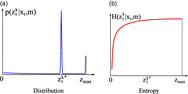
The beam model of the range finders. (a) shows the observation distribution corresponding to four types of measurement errors and (b) illustrates the observation entropy.

The motion control input will affect the observation uncertainty, which in turn determines the localization uncertainty. Therefore, one inspiration is to decrease the observation uncertainty by choosing appropriate actions. In this work, a laser range finder is adopted as the sensor in the robot exploration and we adopt the bean model for the range finder, which incorporates four types of measurement errors, namely the small measurement noise, errors due to unexpected objects, errors due to failures to detect objects, and random unexplained noise [Reference Thrun, Burgard and Fox31]. The measurement probability is then given by
 \begin{equation}\begin{aligned}&p\left(z_t^k|x_t,m\right) = \sum_{i=1}^4 \omega_i*p_i\left(z_t^k|x_t,m\right),\\\end{aligned}\end{equation}
where
 \begin{align*} p_1\left(z_t^k|x_t,m\right) & =\begin{cases}\eta_1\mathcal{N}\left(z_t^k;\,z_t^{k*},\sigma^2\right),\quad \text{if $z_t^k\in\left[0,z_{\max}\right]$},\\[4pt] 0,\quad \text{otherwise};\\ \end{cases}\\[4pt] p_2\left(z_t^k|x_t,m\right) & =\begin{cases}\eta_2\lambda e^{-\lambda z_t^k} ,\quad \text{if $z_t^k\in\left[0,z_t^{k*}\right]$},\\[4pt] 0,\quad \text{otherwise};\\ \end{cases}\\[4pt] p_3\left(z_t^k|x_t,m\right) & =\begin{cases}1,\quad \text{if $z_t^k=z_{\max}$},\\[4pt] 0,\quad \text{otherwise};\\ \end{cases}\text{and} \\[4pt] p_4\left(z_t^k|x_t,m\right)&=\begin{cases}\dfrac{1}{z_{\max}},\quad \text{if $z_t^k\in\left[0,z_{\max}\right]$},\\[8pt] 0,\quad \text{otherwise}.\\ \end{cases}\end{align*}
In the above formula,
 $z_{\max}$
represents the maximum sensor distance, and
 $z_t^{k*}$
represents the real distance of the object measured by
 $z_t^k$
.
An illustration of the measurement probability is given in Fig. 2(a) and its entropy is shown in Fig. 2. It can be proved that a larger measurement distance corresponds to higher uncertainty. In this article, we propose the observation approximation method on the basis of these findings.
4. Methodology
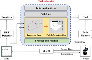
In this section, we first introduce the outline of the proposed robot exploration framework, as shown in Fig. 3. At the beginning, the robot is in an environment without any prior knowledge. The surrounding environmental information is perceived by the equipped sensors. Then, a simultaneous localization and mapping(SLAM) module is employed to receive sensor data, which is utilized to update the map and localize the robot. To extract the frontiers, two RRT trees [Reference Umari and Mukhopadhyay17] are grown in the free area of the updated map. The mean-shift algorithm [Reference Comaniciu and Meer32] is used to cluster the extracted frontiers. At the same time, the grid state of each frontier will be continuously detected. If the pixel value of a grid is less than a given threshold value, they will be removed as invalid points. After that, a new revenue model is constructed for the frontiers, which not only considers information gain
 $I_f$
and path cost
 $N_f$
, but also integrates the consideration of the environmental information on the exploration path, including path information and frontiers information. The candidate frontiers are also constrained by the path distance, which ensures that the robot explores within a limited range while reducing the backtracking problem. In the decision-making stage, the revenue value of each candidate frontier is calculated according to the proposed model and the frontier with the largest revenue value is selected as the target point. After that, the path planning module is activated to generate a path from the current pose to the target point. The above steps will be repeated until the whole environment exploration is completed.
Overall framework of the robot exploration algorithm.

The construction of the revenue model will be further explained in detail in the proposed decision-making strategy. Firstly, the perception area estimation with a given path and map is presented in Section 4.1. Then, the environmental information from the current robot pose to the target frontier is estimated, which is presented in Section 4.2. Finally, in Section 4.3, the proposed revenue model is formulated and combined with the estimated path information gain.
4.1. Estimating the perception area S
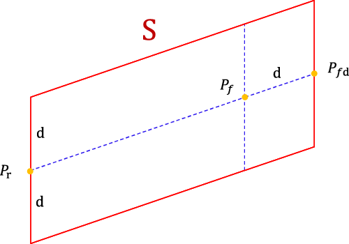
When selecting the target frontier, the perception area that the robot can observe during the process of exploration is firstly estimated, as shown in Fig. 4. In this study, the path from the current robot pose to the frontier is simplified as the line segment
 $\overline{{P_r}{P_f}}$
. d is the detection range of the robot sensor and
 $P_{fd}$
is obtained by extending the distance d of
 $P_f$
along a straight line
 $\overline{{P_r}{P_f}}$
. Because the sensing range of the robot is a sector, the region formed by the sector translation to the frontier can be approximately expressed as the perception area of the exploration process, so the estimated perception area
S
is defined as the parallelogram obtained by swelling the line segment
 $\overline{{P_r}{P_{fd}}}$
to both sides with a distance of d.
The estimated parallelogram region
S
observed by the robot during its moving to the frontier.
 $P_r$
and
 $P_f$
are the positions of robot and frontier, respectively. d is the sensing range of the robot sensor,
 $P_{fd}$
is obtained by extending the distance d of
 $P_f$
along a straight line
 $\overline{{P_r}{P_f}}$
.

4.2. Path information gain estimation
Each candidate frontier corresponds to one path and one perception area. Since the perception area may contain various obstacles, the information gained on the candidate path depends on the environmental information in the perception area. To calculate the environmental information on the path, one idea is to estimate the perception of the sensor during the moving of the robot from the current pose to the candidate frontier. Therefore, the path information gain estimation method is proposed and the information gain is defined as:
 \begin{equation}\begin{aligned}\mathcal{I}_{p} = \sum_{x_t\in \textbf{x}_e} (E_i(x_t, S)+ E_j(x_t, S)),\\\end{aligned}\end{equation}
where
 $E_i$
and
 $E_j$
extract the effective grids that help reduce localization and perceptual uncertainty concerning the horizontal axis and the vertical axis, respectively. For better illustration, we define the terms used in the process as follows:
Definition 1 (Effective Grids). Generally, a grid map has three states: occupied, free, and unknown. Since only occupied grids help for localization, effective grids refer to occupied grids. In addition, when the sensor detects obstacles with a thickness in area S , it will only perceive the minimum distance to the obstacle. In this way, the thickness of the obstacle cannot help the perception process and the corresponding grids are considered invalid.
The path information gain outputs the number of effective grids. The more the number of effective grids, the more obstacles, and the richer the environmental information.
Definition 2 (Grids Traversal). The process of checking each grid state one by one in the estimated perception area. If the grid is occupied, the effective grid is increased by one.
Definition 3
(Traversal interval). The interval of each traversal is a unit length in the grid coordinate system, which is related to the map resolution. For example, in the grid coordinate system, i and j are used to represent the horizontal axis and the vertical axis, respectively, so the interval of traversal is
 $(i_{1}+1)-i$
 $_1$
.
Because the number of effective grids obtained by simply traversing along the vertical or horizontal axis in the estimated perception area is not accurate, there are some omissions, so we calculate from two directions, and do not count the repeated traversed grids.
In the effective grid extraction process, we traverse the points in the area
S
along the line segment
 $\overline{{P_r}{P_{fd}}}$
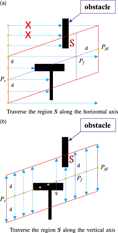
from the horizontal and vertical axes, respectively. As shown in Fig. 5(a), when traversing along the horizontal axis, the line segment
 $\overline{{P_r}{P_{fd}}}$
can be formulated as
 ${j=k*i+b}$
. The i axis intercept of the two lines after translating d is
 ${b_1=b+d}$
,
 ${b_2=b-d}$
. These two lines form the upper and lower edges of the parallelogram region. Suppose the current pose of the robot
 $x_t=(i_1,j_1)$
and the extension of the candidate frontier
 $P_{fd}=(i_2,j_2)$
. The ordinate of a point in a parallelogram region can be expressed as
 $J =\{j_1-d,\ \cdots,\ j_1-1,\ j_1, \ j_1+1,\cdots,\ j_2+d \}$
 $(take \ j_1<j_2 \ as \ an \ example)$
. For each
 $j\in J$
, a series of grids can be extracted in
S
with to the direction of
 $\overrightarrow {{i_1}{i_2}}$
, namely
 $\left({i_k},{j_k} \right),\ k=1,2,\ldots$
. The grids in this set are checked and if they are occupied, the traversal in this row will be terminated due to the remaining grids in this row are not effective grids. The traversal lines are represented with dotted lines in Fig. 5(a).
Calculate the number of effective environmental information in area S . Figure (a) and (b) traverse the region along the horizontal axis and vertical axis, respectively. The black column in the figure represents the obstacle, and the arrow indicates the direction of traversal. Each small orange dot represents a grid coordinate with an interval of one unit length. The red “X” means that even if obstacles are traversed along this direction, they are not counted because they are not in area S .

When traversing along the vertical axis, as shown in Fig. 5(b), the abscissa of each point on the line
 $\overline{{P_r}{P_{fd}}}$
is then represented as
 $I =\{i_1,i_1+1,i_1+2,\cdots,\ i_2\ \}$
. Each point
 $\left({i_k},{j_k} \right)$
on the line segment is translated upward and downward by a distance d, respectively. When the grid is occupied, the traversal in this direction is terminated. After the completion of the traversal in the upper and lower directions, we turn to the next point and repeat the above steps until the traversal of the points on the whole line segment is completed. Similarly, for a straight line parallel to the coordinate axis, the area
S
obtained by translating the distance d along the straight line to both sides is a rectangle, and it is relatively simple to traverse the region
S
along the straight line, which will not be repeated here.
4.3. Revenue modeling with path information gain
In this part, a new revenue model is constructed for frontier selection, which includes the following factors.
• Information Gain (
 $\textbf{I}_f$
): the number of unknown grids in the circle with radius r centered of a frontier.
• Path Cost (
$\textbf{N}_f$
): the Euclidean distance between the current position of the robot and the position of the frontier.• Path Information Gain (
$\mathcal{I}_{p}$
): the number of effective grids in the estimated perception area
S
, which represents the richness of the environmental information.• Frontiers Information (
$\textbf{O}_f$
): the number of occupied grids in the circle with radius r centered of a frontier.


The revenue function is defined as:
 \begin{equation}\begin{aligned}R_f= h_1\ast I_f- N_f+ h_2\ast\mathcal{I}_{p}+O_f,\\\end{aligned}\end{equation}
where
 \begin{equation}h_1 =\begin{cases}\delta,& d_{1}< c_1\ \text{or}\ d_1 > c_2,\\[5pt]1,& \text{otherwise}.\end{cases}\end{equation}
and
 \begin{equation}h_2 =\begin{cases}\zeta,& {d}_1 < {c}_1\ \text{or}\ {d}_1 > {c}_2 ,\\[5pt]c / d_1,& \text{otherwise}.\end{cases}\end{equation}
Herein, to reduce the repeated exploration and guide the robot to explore adjacent areas, we constrain the function with two parameters according to the length of the exploration path. As shown in Equations (10) and (11),
 $d_1$
is the Euclidean distance between the current position of the robot and the position of frontier; c,
 $c_1$
, and
 $c_2$
are empirically set.
 $\delta$
and
 $\zeta$
are set as
 $\delta\le0.1$
and
 $\zeta\le0.01$
, respectively, which can help avoid the robot staying in place due to the maximum profit value of a certain target point. In addition, it can also make the robot search in a limited range and avoid the backtracking phenomenon.
The balance between reducing trajectory uncertainty and exploring new areas is a classic problem in robot exploration. In this work, we focus on the scenario that the environment structure is beyond the range of sensor perception. If the robot selects a target frontier that is biased toward information gain, the trajectory uncertainty may increase and the robot cannot effectively update the target area with limited perception, which may cause the robot to linger in this blank area for a long time. When selecting the frontiers with abundant environmental information, the trajectory uncertainty may decreases, however, the update speed of the unknown area of the map reduces. In this work, we carry out a lot of experiments to determine the proportion of each composition in the revenue model to balance the weights of information gain and trajectory uncertainty. When each frontier contains rich environmental information, the robot will still be more inclined to explore the unknown area. Under perceptual uncertainty, most of the phenomenon of robot wandering in empty areas can be solved, and the exploration efficiency can also be significantly improved.
5. Experimental studies and results
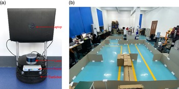
To verify the effectiveness of our proposed robot exploration method, both simulations and real-world experimental studies are carried out and a laptop computer with Intel Core i7-9750H CPU @2.6 GHz and 16 GB RAM is adopted as the computing platform. In the real-world experimental studies, the Turtlebot mobile robot platform equipped with a Velodyne lidar is adopted, as shown in Fig. 6. The RRT-based robot exploration algorithm [Reference Umari and Mukhopadhyay17] is adopted as a reference. The experiments have been divided into two parts, namely the frontier selection experiments and the robot exploration experiments.
Robot platform in the real-world experimental studies. (a) Setup of the robot platform; (b) real-world scenario.

5.1. Frontier selection
In the first part, we develop the modified algorithm using MATLAB to intuitively show the performance of the frontier selection. During the experiment, the partially known map and the current robot pose are given. The perception model of a laser rangefinder with
 $180^{\circ}$
fields of view is adopted and its detection range is set according to the environment size. A set of candidate frontiers are also presented. According to the different revenue models formed by our algorithm and the RRT-based algorithm, the target frontier can be then obtained.
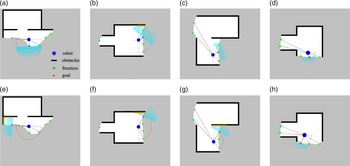
Four groups of the experimental results are shown in Fig. 7, in which the robot is in an environment where solid obstacles are beyond its sensing range, and the sensing range of the laser rangefinder is represented by a semicircle with dotted lines. The target points selected by the RRT-based algorithm are shown in Fig. 7(a)–(d), while those selected by our method are shown in Fig. 7(e)–(h). Obviously, the target point selected by our method contains more abundant environmental information and will guide the robot to move with less perceptual uncertainty, although the update speed of the unknown area of the map at the current time is low, it can effectively avoid wandering in the empty area.
Selection of the target frontier. (a)–(d) denote the performance of the RRT-based method while (e)–(h) denote that of the proposed method. The blue dot indicates the position of the robot, the semicircle dotted line indicates the sensing range, the green squares represent the frontiers, and the red five-pointed stars indicate the selected target point.

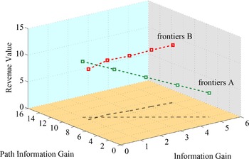
The proposed method makes a trade-off between exploring new areas and reducing uncertainty. To further analyze the proposed revenue function, we also record the extreme value distribution in the revenue function with respect to two groups of frontiers. As shown in Fig. 8, the frontiers of group A are collected from a poorly perceived environment, while the frontiers of group B are collected from a well-perceived environment. For the frontiers of group A, as the information gain increases, the path information gain decreases, which means a larger trajectory uncertainty. In this case, the revenue value also decreases since the trajectory uncertainty dominates. Therefore, the robot still tends to choose the frontier with richer environmental information. On the contrary, when there is little difference in the environmental information contained in the frontiers, as shown in group B, the revenue value is mainly determined by the information gain of the unknown region, and the robot is then more inclined to explore the unknown area.
Revenue function analysis with respect to two groups of frontiers.

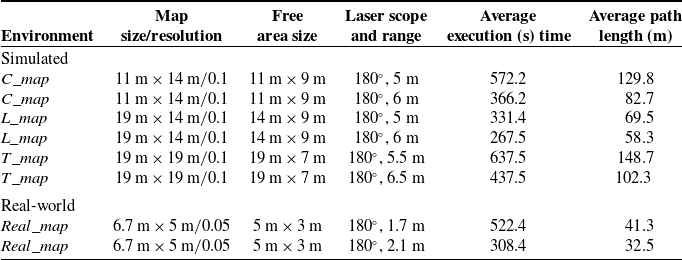
Statistics of our robot exploration method in simulation and real experiments.

5.2. Exploration performance
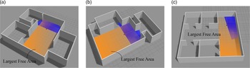
In this part, the experiment is conducted based on the Robot Operating System (ROS) [Reference Quigley, Gerkey, Conley, Faust, Foote, Leibs, Berger, Wheeler and Ng33]. Three simulated environments and one real-world environment are included, as shown in Figs. 6 and 9, respectively. For each environment, two kinds of laser sensing range are tested, which generates 8 scenarios and the corresponding settings in each scenario are listed in Table I. Herein, the free area size refers to the size of the largest rectangle free area A in the environment, as shown in Fig. 9, which is utilized to determine the sensing range of the laser range finder in each scenario. Let the width of the largest rectangle be
 $l_{\max}$
and let the sensing range of the laser range finder be r, which is obtained as follows:
 \begin{equation}\begin{aligned}r=\left\lfloor \frac{l_{\max}}{2\sin \theta}\right\rfloor,\\\end{aligned}\end{equation}
where the function
 $\lfloor x\rfloor$
rounds x to the nearest integer and
 $\theta$
is utilized to adjust the perception uncertainty. The idea is that when the robot is in the middle of A, namely with the largest perception uncertainty, the effective perception rate of the robot can be calculated by
 $\frac{\theta_{\max}-2\theta}{\theta_{\max}}$
, where
 $\theta_{\max}$
denotes the angular scope of the laser ranger finder. In this work,
 $\theta_{\max}$
is set as
 $180^{\circ}$
. To exhibit the ability of the exploration algorithm to deal with perceptual uncertainty, we select two effective perception rates for evaluation, namely
 $\frac{1}{3}$
and
 $\frac{1}{2}$
and then we can determine the sensing range of the laser in each scenario. Therefore, in the
 $C\_map$
and the
 $L\_map$
scenario, the sensing range of the laser is set as 5 and 6 m, respectively. Similarly, in the real-world scenario, the sensing range of the laser is set as
 $1.7$
and
 $2.1$
m, respectively. For the
 $T\_map$
scenario, which is more empty compared with the previous two environments, we compare the experiment in the perception range of
 $6.5$
and
 $5.5$
m, respectively.
Robot exploration simulation scenarios. (a) C
 $\_$
map; (b) L
 $\_$
map; (c) T
 $\_$
map.

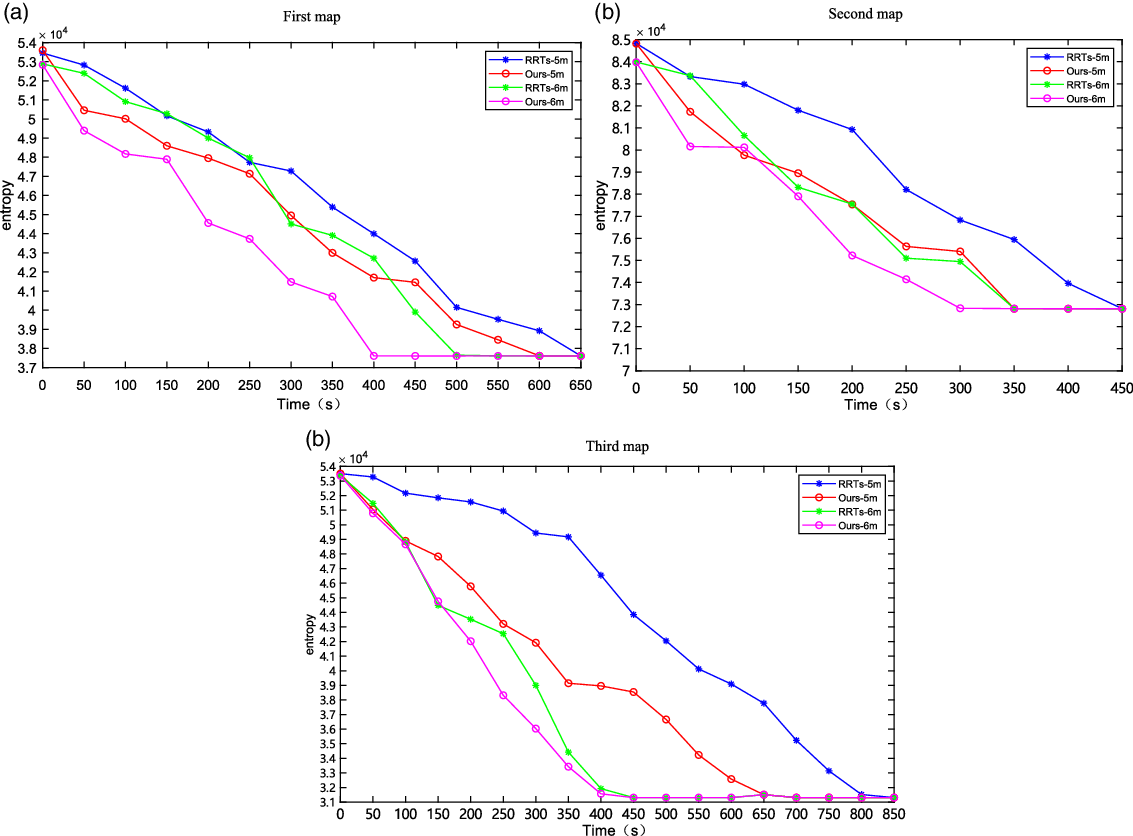
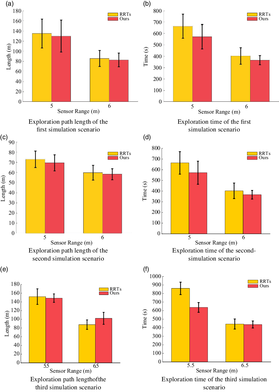
We record the map entropy in three simulation scenarios, as shown in Fig. 10. In the process, we record the data every 50 s and compare it with that of the RRT algorithm concerning different sensing ranges. From the attenuation curve of map entropy, we can see that the map entropy of our method reduces faster, which shows the effectiveness of the proposed method in robot exploration. To further compare the performance of the two algorithms, 10 times repeated trials are conducted for each method in each scenario. The runtime and path length of the robot during the exploration are recorded, as shown in Fig. 11. The experimental results show that in the first map when the sensing range is 5 m, our method reduces the exploration time by 13.8
 $\%$
and the length of the exploration path by 3.8
 $\%$
compared with the RRT-based algorithm. When the sensing range is 6 m, the exploration time is reduced by 9
 $\%$
and the length of the exploration path is reduced by 2.5
 $\%$
. In the second map, when the sensing range is 5 m, our method reduces the exploration time by 21.1
 $\%$
and the exploration path length by 4.7
 $\%$
compared with the RRT-based algorithm. When the sensing range is 6 m, the exploration time is reduced by 14.1
 $\%$
and the length of the exploration path is reduced by 2.6
 $\%$
. In the third map, when the sensing range is 5.5 m, our method reduces the exploration time by 25.9
 $\%$
and the exploration path length by 2.2
 $\%$
compared with the RRT-based algorithm. When the sensing range is 6.5 m, compared with the RRT-based algorithm, our algorithm has no obvious advantage in the exploration time and is slightly inferior to RRTs in the length of the exploration path. Because the width of the empty area of the environment is 7 m, the robot has a good perception of the environment, so our method to select the frontiers with rich environmental information will inevitably travel more distance.
Map entropy reduction in the experimental studies.

Experimental results of the robot exploration. The left shows the length of the robot and the right shows the runtime during the robot exploration.

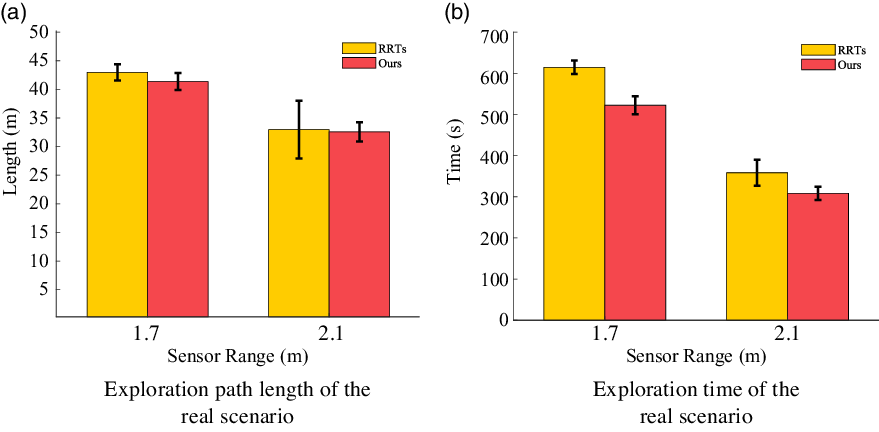
In the real-world scenario, as mentioned earlier, the sensing range of the laser range finder is set as 2.1 and 1.7 m, respectively. We also record the runtime and path length of the robot during the exploration in 10 times repeated trials, as shown in Fig. 12. When the sensing range is 1.7 m, our method reduces the exploration time by 15
 $\%$
and the length of the exploration path by 3.7
 $\%$
compared with the RRT-based algorithm. When the sensing range is 2.1 m, the exploration time is reduced by 13.9
 $\%$
and the length of the exploration path is reduced by 1.2
 $\%$
. However, in most cases, the importance of the exploration time is higher than the path length, so the path length deficiencies in individual scenarios are acceptable.
In all, our method improves the performance of the robot under the uncertainty of perception by selecting the frontiers with rich environmental information. The robustness of our algorithm is proved by comparing experiments in different environments.
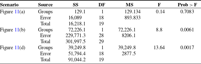
Statistical significance analysis of the scenarios with large variances.

Experimental results of the robot exploration. The left shows the length of the robot and the right shows the runtime during robot exploration.

5.3. Discussions
When the sensing range of the sensor is limited, the positioning uncertainty of the robot increases, resulting in poor map quality. At this time, the difference caused by the selection of different frontiers is more obvious, which leads to fluctuations in the exploration experiments, as shown in Fig. 11(a), (b) and (d). Therefore, we supplemented 10 groups of experiments and carried out statistical significance analysis for these three scenarios.
After adding 10 groups of data, the average value and variance of the experimental data have little change, which shows that the data obtained before and after the test are reasonably floating. The variance of the two kinds of data is still greater than the difference between them. From the statistical results, the experimental error is reasonable and normal. The statistically significant differences between the three groups of comparative data are shown in Table II. In the analysis of variance table, the source column represents intra-group(Groups) variance, inter-group(Error) variance, and total variance, respectively. SS is the sum of squares, DF is the degree of freedom, MS is the mean square deviation, and F value is equal to the ratio of mean square deviation between groups and mean square deviation within groups, which reflects the effect of random error. Prob > F indicates the
P
-value. Herein, we first make a hypothesis that there is no significant difference between the two groups of data in statistics, and then judge whether to accept the original hypothesis according to the
P
-value. When
 $\textbf{P} < 0.05$
, the original hypothesis is rejected, indicating that the sample sets obtained by the two methods have significant differences; otherwise, the original hypothesis is accepted, indicating that there is no significant difference between the two sample sets. As shown in Table II, we can see that the
P
values are 0.7083, 0.0061, and 0.0017, respectively. It can be seen that the two methods have significant differences in the index of time, but no significant differences in the index of the path. In the actual process, the proportion of time is more important than the path, and the average value of the path of the two groups of methods has little difference, so the difference is not obvious. However, after supplementing several groups of data, the average value of the data does not fluctuate much, so we have reason to believe that our data is within a reasonable range and has statistical significance.
6. Conclusions
In this study, a decision-making method for robot exploration based on sampling has been proposed by integrating the estimated path information gain and the frontier information. In the process of selecting frontiers, the estimated environmental information to the candidate frontier is proposed and included, guiding the robot to select a frontier with richer environmental information to improve the exploration efficiency under perceptual uncertainty. The experimental results demonstrate that our method has a significant reduction in exploration time and path length, which further proves the effectiveness of our model. In future work, we plan to optimize the weight distribution of the revenue function based on inverse reinforcement learning, and further improve the efficiency of exploration.
Conflicts of Interest
None.
Financial Support
National Key R
 $\&$
D Program of China No.2019YFB1310003, National Science Foundation of China No.61903267 and China Postdoctoral Science Foundation No.2020M681691.
Ethical Considerations
None.
Authors’ Contributions
None.