1. Introduction

Circulation of the arctic ice cover is affected by ice mechanics, especially in the vicinity of narrow passages through, for example, the canadian arctic archipelago. in this region, particularly the nares Strait, Sea ice tends to flow through into baffin bay in the Summer and fall, but then normally becomes relatively Stationary around november or later in the year. this Stoppage typically occurs in conjunction with the formation of a relatively Static, arch-like Structure with effectively no ice downstream from the ‘arch’. in models with appropriate ice mechanics, that allow uniaxial compressive Strength, it is found that ‘arches’ are mechanically Stable up to Some body-force limit dependent on the ice Strength and the width of the opening. beyond that limit, increases of wind or water body forces on the ice cover can ‘break’ the arch. in practice, once a Stoppage occurs as in the nares Strait, it may be Strengthened by thermodynamic processes, So that its breaking Strength increases with time.

One of the first quantitative analyses of ice arching was made by Reference sodhiSodhi (1977) who examined cases of ice arching occurring in the bering Strait, Sometimes forming as a double arch, with the diomede islands in the center of the Strait providing the common leg of the double arch. Reference sodhiSodhi (1977) noted that these Static arches could be explained by a two-dimensional coulombic granular model, based on analysis first carried out by Reference Richmond and GardnerRichmond and gardner (1962) of wet granular flow through cylinders. two important features of this granular analysis were that (1) cohesive Strength (the ability to Sustain uniaxial Stress) is needed for the formation of a Static arch, and (2) the Static arching problem is inherently indeterminate due to the uncertainty in the Shape of the arch which may form. however, by examining different Shapes of arches, Reference Richmond and GardnerRichmond and gardner (1962) were able to establish the minimum passage width that could Sustain flow for a fixed forcing, and maximum passage widths that might Stop flow for a fixed forcing and cohesive Strength.

In the case of passages out of the arctic basin, the problem is complicated by thermodynamic processes which can effectively create larger or lesser amounts of ice flowing into a narrow passage. this argument also applies to the arctic basin as a whole Since equilibrium thickness depends non-linearly upon residence time, ice growth and decay and ice outflow. in terms of outflow, the arctic Sea ice differs Significantly from antarctic Sea ice Since a Series of islands and continents (fig. 1) constrain the arctic ice cover to an enclosed basin with a Series of outflow passages varying in Size, with Some of the Smallest occurring in the canadian arctic archipelago, while fram Strait forms the largest. Some of these passages often Seasonally Stop ice flow, while others, Such as fram Strait, Seasonally reduce their flow under the Same forcing conditions.

Fig. 1.

Arctic basin 40 km grid. Letters denote passages where ice may exit the Arctic basin which in this grid are treated by zero-strength open boundary conditions. F is Fram Strait, B is the Bering Strait, SP and L are passages either Side of Franz Josef Land, and S is the passage to the west of Severnaya Zemya.

This indicates that multiple flow States of the arctic Sea-ice cover induced by ice mechanics can exist, with one State being a largely thermodynamic equilibrium State with the ice outflow essentially jammed up at the passages. the other State would consist of a thickness balanced by a large outflow together with net growth over the ice cover balancing the outflow. the existence of this multiple equilibrium climate State, with the idealized case of only one outflow passage together with mean monthly wind forcing, was demonstrated earlier by Reference Hibler, Hutchings, V.A. and LanghorneHibler and hutchings (2003). in this complementary Study, we examine the case of a realistic arctic basin with multiple passages, and focus on the Seasonal Stoppage of ice with realistic daily wind forcing. in addition, the effects of different rheologies on the potential of multiple flow States are examined.

2. Characteristics of PLastic Flow Through Narrow Passages: The Effect of Rheology

Static ‘arching’ or Stoppage of a plastic material can be treated by a variety of analyses ranging from a coulombic granular analysis (Reference Richmond and GardnerRichmond and gardner, 1962) to a thick-walled concentric elastic–plastic analysis (Reference Pritchard, Reimer and CoonPritchard and others, 1979). independent of the particular analysis, it is easy to See, by considering continuity of Stresses along a free two-dimensional Surface, that a Stationary arch requires the presence of uniaxial compressive Strength or, in terms of granular material nomenclature, the presence of cohesive Strength.

While the cohesive Strength concept gives Some insight into the limiting flow characteristics through narrow channels, complete analysis of the plastic flow requires understanding the behavior of the flow as the arching limit is approached. with the appropriate Scaling, this flow can be numerically analyzed in a non-dimensional manner (Reference IpIp, 1993). consider a tapered channel as in figure 2, with parameters: width of the opening λ, ice Strength P and wind Stress т = ρ _a c _a u _g ². for this System the x momentum equation in the absence of coriolis force is given by

Fig. 2.

Idealized narrowing channel used for flow calculations. Shaded regions denote open boundary conditions.

(1)

Where u is ice velocity, u _g is geostrophic wind velocity, c _a and c _w are air and water drag coefficients, and σxx and σxy are components of ice Stress, which are a non-linear function of the Spatial gradients of u (Reference HiblerHibler 1979). expressing x and y in terms of λ and Stress in terms of P, we have, after dividing by the wind Stress, the dimensionless equation

(2)

Where x and y are dimensionless, and β and ϒ are dimensionless parameters:

(3)

To examine the character of the flow, we consider a 50 by 50, 40 km resolution grid as Shown in figure 2. the Shaded bands Show regions where zero ice Strength is assumed So the ice can freely flow into or away from these bands. a constant Stress of т = 0.4 nm^–2 in the direction of the arrow is used for the body force. to Simplify Scaling, a linear water drag is used with ρ _w c _w = 0.56 kgm^–3. for a plastic rheology the modified coulombic yield curve of Reference Hibler and SchulsonHibler and Schulson (2000) is utilized. this rheology has the requisite uniaxial compressive Stress needed for Static arching, which for a coulombic rheology requires Some tensile Stress. we Solve the equations of motion, for u, using the finite differences and relaxation procedure of Reference HiblerHibler (1979). ice Strength is taken to Scale linearly with thickness according to P = 4 ×104h.

figure 3 Shows a dimensional plot of mean ice velocity and ice export as a function of ice thickness, or equivalently ice Strength. Since linear water drag is used, the Same mean velocity curve will apply in non-dimensional form (verified by Simulation), with the abscissa being ϒ=P/λт and the ordinate being the basic character of the Solutions is a gradual decrease of the ice velocity as the Strength increases or the opening Span (λ) decreases. at Some point, the velocity becomes zero and an effectively Static Solution with an arch is obtained. the System is close to motionless, with higher velocities existing in an arch-shaped region near the outflow opening. with no ice interaction, the ice velocity is a constant fraction of the wind Speed.

Fig. 3.

Average ice velocity and mass outflow for a fixed forcing applied to the narrowing channel in Figure 2 as a function of ice thickness or equivalently ice Strength. The modified coulombic rheology of Reference Hibler and SchulsonHibler and Schulson (2000) was utilized here. The quantity plotted has units ms^–1, and requires a conversion factor of 42 000m to obtain areal outflow in m² S^–1.

The ice outflow is particularly relevant to the multiple equilibrium problem. Since ice Strength Scales with thickness, the outflow peaks for intermediate values of the flow where both the velocity and thickness are Significant. it can be Shown that the appropriate non-dimensional outflow, call it , Scales as α ∽(P/т ²)Δ, where Δ is the outflow in dimensional form.

An important aspect of the outflow is that the non-dimensional form of the velocity and mass outflow curves depends on the rheology, primarily on the magnitude of cohesive Strength. this is illustrated in figure 4, where non-dimensional velocities are plotted for a number of different rheologies. we have plotted the velocity for an elliptical yield curve, a coulombic rheology without cohesive Strength (classic mohr–coulomb), Sine-lens yield curve and a cavitating fluid. the non-dimensional velocity goes to a final Stoppage at a larger Strength (or Smaller opening) for yield curves crossing the principal axes nearer the origin. this means yield curves with more cohesive Strength (ellipse) Stop ice flow through passages at lower Strength or larger opening than yield curves with less cohesive Strength (modified coulombic). in the case of no cohesive Strength (mohr–coulomb), there never is Stoppage, although the flow Slows down considerably. finally, for the cavitating fluid case, there is Some reduction of flow due to the constraining of the passage, but generally the flow continues for all Stress States. consequently, a cavitating fluid model would have no capability to Stop ice flow through the canadian arctic archipelago if the passages were resolved. conversely, the excessive amount of Shear Strengths in certain elliptical yield curves could jam up the flow through fram Strait.

Fig. 4.

Non-dimensional ice outflow through the channel in Figure 2 for different rheologies.

3. Multiple Flow States of The Arctic Ice Cover DUE TO Ice Mechanics

To examine the potential of multiple flow States through outlet passages induced by ice mechanics for the arctic Sea-ice cover, we need to consider the potential of the multiple passages through which Sea ice can exit and enter. indeed the most notable Set of passages with regard to Stoppage are those through the canadian arctic archipelago which historically, in winter, have been largely Stopped but may be beginning to become more porous to Sea ice. as there are multiple passages, it may be possible to achieve many ‘equilibrium’ States due to certain passages (such as the archipelago) being blocked while others are relatively open. here we consider the archipelago to be closed, and examine the remaining passages consisting of a Series of passages between islands and peninsulas Separating the arctic basin from the barents Sea.

To examine the outflow, we carry out a Simulation with a Stand-alone Sea-ice model without ocean circulation, described in detail by Reference Hibler, Roberts, Heil, Proshutinsky, Simmons and LovickHibler and others (2006) in a Study of M2 tidal forcing. this Simulation uses the grid Shown in figure 1 with Spatially random Strengths, and zero-strength boundary conditions at the outflow cells. a 201 S time-step was chosen Such that the M2 tidal period is divisible by the time-step length (Reference Hibler, Roberts, Heil, Proshutinsky, Simmons and LovickHibler and others, 2006), although tides were not included in the Simulations presented in this paper. a Short time-step is required to ensure the ice velocity Solution approaches plastic equilibrium over a Shorter time period than the evolution of the internal ice Stress field due to forcing. interpolated 6 hourly wind data from european centre for medium-range weather forecasts (ECMWF) forcing for 225 days beginning with 1 october 2001 were used as forcing to a Stand-alone viscous–plastic Sea-ice model. figure 5 Shows the general character of the outflow area variability for the passages identified in figure 1. a Striking characteristic is the extreme variability in the outflow over the modeled timescale (see fig. 6b). consequently we See that at any one location there will be considerable variation in Standard deviation in the flow both in and out of the arctic. it is also notable that the variability of the flow through passages f, Sl and l is quite Similar.

Fig. 5.

Time Series of areal outflow (with units ms^–1, as in Fig. 3) through four passages, F, SP, L and S, identified in Figure 1 for (a) thin and (b) thick initialized Simulations. A temporally constant ice Strength with random Spatial variability was used for the Simulations here over a ∽220 day period beginning on 1 October 2001. Note that in (a) results are Shown from two Simulations initialized with 1 m and 2 m thick ice. Both 1 m and 2 m Simulations in (a) converge to identical States, and the 2 m initialized Simulation has greater outflow through all passages than the 1m initialized Simulation, on approach to equilibrium.

Fig. 6.

(a) Average outflow (with units ms^–1, as in Fig. 3) and (b) Standard deviation of outflow through all the passages denoted in Figure 1 over ∽220 day period Shown in Figure 5a outflows (thin initialized Simulation). The total of all passages is also Shown.

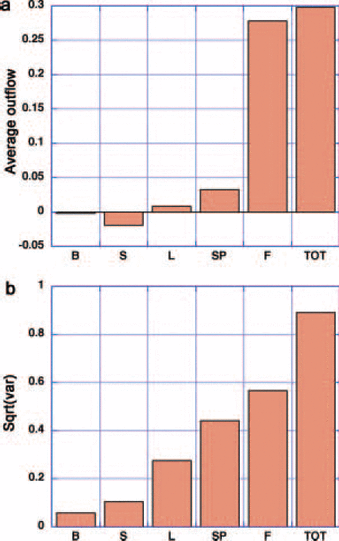
While the variability of the flow through these passages is quite Similar, the geometry of the arctic basin together with the typical wind Structure nevertheless conspires to cause much of the mean flow to be through fram Strait, when ice mechanics is included in the model. this is Shown in figure 6, which Summarizes the modeled mean flow and Standard deviation of the flow through the five passages, together with the total outflow. when the highly variable flow is averaged over this period, the flow through most of the passages averages out to zero So that the total outflow (fig. 6a) is closely approximated by the flow through fram Strait, with net areal flow through all the other passages an order of magnitude Smaller. the Standard deviation of the flows through all passages (fig. 6b) is, however, much closer to the fram Strait Standard deviation, and is Somewhat enhanced due to the Standard deviation being taken about zero. particularly notable is the variability of flow through the passages on either Side of franz josef land (sp and l in fig. 1), passage l also being a region of high ocean transport into the basin.

We examined outflow and the potential for multiple equilibrium States under perpetual winter conditions. the model was forced with an instantaneous wind (1400 h on 1 october 2001) when there is positive outflow for all passages except the bering Strait. we then examine the mass outflow (fig. 7) for increasing ice thicknesses in a manner Similar to that done for the idealized channel in figure 2. as can be Seen from figure 7a, the total outflow and the fram Strait outflow Show the classic peaked pattern very Similar to that through an idealized channel. the main difference, due to this particular choice of wind field, is that the fram Strait outflow is about one-third of the total outflow even though its Shape vs Strength (i.e. ice thickness) is much the Same.

Fig. 7.

(a) Total and Fram Strait outflow vs ice thickness for a fixed wind forcing. (b) Total outflow and basin-averaged growth rates for fixed Spatially constant ice thicknesses and fixed wind forcing. The units of outflow are m² S^–1, and can be converted to m³ S^–1 with a conversion factor of 42 000 m. The units of growth rate are m² S^–1 and have been normalized by 42 000 m.

To estimate the potential for multiple flow States, the key Step is to estimate growth rates over the basin on the Same Scale as the mass outflow. using the idealized Reference ThorndikeThorndike (1992) thermodynamic model plus winter ice-growth estimates from Reference Thorndike, Rothrock, Maykut and ColonyThorndike and others (1975), we estimate typical growth rates as Shown in the intersecting growth curve and mass outflow curve in figurefigure 7b. these two curves (growth and outflow) plotted against a State variable, here taken as thickness, or equivalently ice Strength, form the diagnostic for the presence of multiple equilibrium States (for this particular fixed forcing). note that the addition of outflow channels increases the mass outflow as compared to Simulations with only fram Strait open. hence, for the Same growth rate function, the addition of outflow channels actually increases the possibility of multiple States. for a Simulation with only fram Strait outflow, lower growth rates are required to lower the growth curve to intersect the reduced outflow curve at more than one point.

(4)

While all three intersection points where growth matches outflow are candidates for equilibrium States, only two (1 and 3) are Stable, as can be easily Seen by a local linear Stability analysis about the equilibrium points. in particular, the rate of change of ice thickness is given by

Where G(h) is the growth rate and O(h) is the outflow rate. considering h _o to be a Solution of this equation and h ₁ = h – h _o a Small thickness perturbation relative to h _o, expanding G and O in a taylor Series expansion about h _o, the rate of change of the perturbation to lowest order is

(5)

Where G ^'(h) = dG/dh and O ^'(h) = dO/dh. clearly the Small perturbation will grow unless [G ^'(h)–O ^'(h)] < 0, a condition which, by inspection of figure 7b, is met for Solutions (1) and (3) but not for Solution (2). a physical explanation follows that at points 1–3 the outflow balances ice growth. perturbing the ice to a Slightly thicker (thinner) State at points 1 and 3, the outflow exceeds (is less than) growth Such that the System is driven back to the equilibrium point. hence points 1 and 3 are Stable. however, perturbing the ice at point 2 to a thicker (thinner) State results in ice growth exceeding (less than) outflow, Such that the System is driven to the thicker (thinner) equilibrium point. as Solution (2) is not Stable, as one proceeds from a cold climate to a warm climate there will be a rapid jump to a lower thickness State which then changes less rapidly with warming.

To assess the existence of actual multiple equilibrium States, we add advection and growth to the Sea-ice model and initialize it with 1 m and 6m of ice. integrating these two cases forward in time, we See the natural evolution of two equilibrium States as illustrated by the evolution of thickness at a fixed gridcell in the basin in figure 8. note that in the thin Solution the evolution of the thickness is relatively complex. ice build-up modifies the local ice flow Such that the outflows through different passages may differ from each other and in time, especially for passages that are Sustaining flow. this occurs even though the forcing and thermodynamics are Smooth, and demonstrates the nonlinearities inherent in the ice rheology, especially when coupled to even a Simple thickness distribution model.

Fig. 8.

Ice thickness at gridcell (50,60) (see Fig. 1) vs time for the (a) thin and (b) thick initialized Simulations including ice growth and advection with a fixed wind forcing. In (a) two Simulations are Shown initialized with 1m (red Solid line) and 2m (blue dashed line) thick ice. In (b) two Simulations are Shown initialized with 6m (blue Solid line) and 8m (red dashed line) thick ice.

The gradual modification of flow through different passages is illustrated in figure 5, which Shows the evolution of mass outflow through all the passages. for this forcing, the chief characteristic is that the outflow is dominated by passages on either Side of franz josef land (passages l and Sp). the S passage flow is initially Small and remains Small. however, note that, while initially Substantial, the fram Strait passage outflow is gradually Shut off by the buildup of ice. note also that the timescale for this build-up and flow reduction is of the order of 1 year or less.

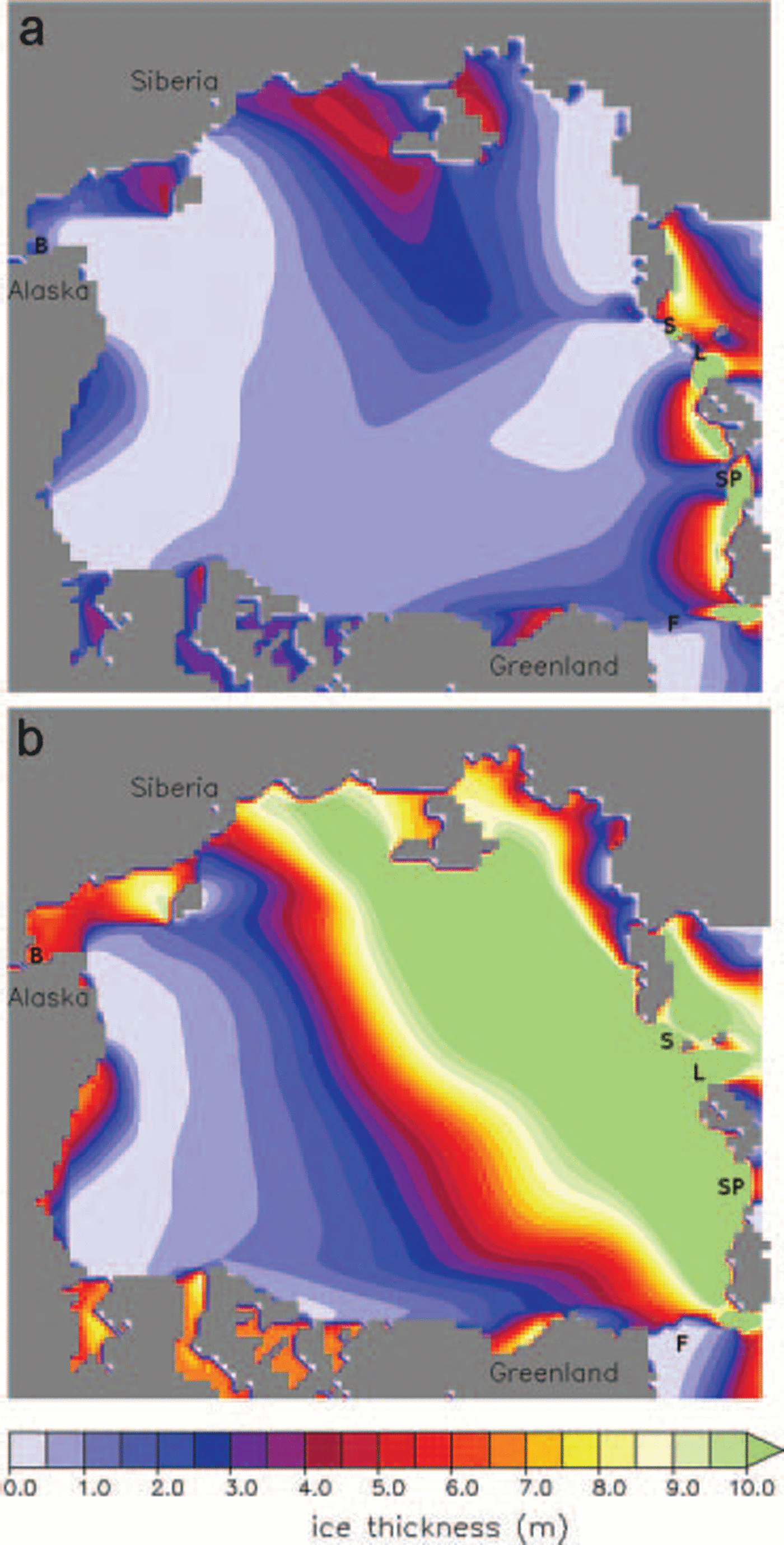
This dominance of two passages in the outflow can be Seen in figure 6a, and the ‘thin’ ice-thickness characteristics Shown in figure 9a. in the case of the thin Solution, the ice build-up gradually develops Such that passages l and Sp remain open while fram Strait is largely closed off. this can be contrasted to the ice build-up in the thick case (fig. 9b), where ice builds up into a Smooth wall along the arctic ocean Side of all the passages, essentially Separating the arctic basin ice pack from the bering and greenland Sea. in this case, the Strength is too great for flow through passages to ever occur.

Fig. 9.

Thickness contours for (a) the thin initialized Simulation and (b) the thick initialized Simulation halfway through each Simulation.

4. DIsCUssIon and Conclusions

The main focus of this paper has been the Seasonal Stoppage or reduction of ice flow through narrow passages which collectively constrain the arctic Sea-ice cover to an enclosed basin. a Secondary focus has been the effects of climate change on flow States through these passages, and the potential for a Shift to a higher flow State as the ice cover becomes thinner and weaker due to warming. it is because we assume a cooler climate and perpetual winter in our model that we can Simulate ice arching at fram Strait. for our purposes, we have used larger passages from the basin as analogues (under a cooler climate) to narrower passages which require a considerably warmer State to Switch to a high flow State.

Analysis of the effect of rheology on flow of Sea ice through passages Shows the cohesive Strength Supported by the ice pack is critical in allowing ice arches to form across a passage. in addition, even without cohesive Strength, a large Shear Strength can reduce outflow through passages. if the ice pack has Substantial Shear Strength that approaches cohesive Strength, the mass flow through a passage displays a highly peaked character, with the flow peaking at Some mean ice thickness and then decreasing as the thickness increases further. with a model that has true cohesive Strength, as ice thickness increases the flow eventually totally Stops.

When thermodynamics are added to this non-linear process model for outflow through narrow passages, the potential for multiple flow States is introduced as Seen in figure 7b. the ‘rapid’ flow State occurs because the increased mass flow at lower Strengths can balance the higher growth rates. the ‘reduced’ or low flow State occurs when high Shear Strength in conjunction with thicker and Stronger ice Slows the ice mass flow through passages. the thicker ice has a reduced ice growth which compensates for the reduced outflow. in the extrema, i.e. models with no Shear Strength, as in a cavitating fluid, this low flow Solution is not possible, and multiple equilibrium States are not present.

Application of a numerical Simulation to the larger passages of the arctic Shows that fluctuating wind fields and high forcing do not Significantly alter the balance in the formation of two States. we find the balance between outflow and ice growth, and the presence of multiple equilibrium Solutions, can be deduced from numerical experiments with relatively Steady forcing. these Simulations can demonstrate how close to the threshold of multiple flow States, through all the passages of the arctic basin, the ice pack has been in recent times. our results indicate that Simulating Sea ice, with realistically large ice Strengths, over the last-half century is an initial-value problem that is Sensitive to ice thickness.