1 Introduction
Particle-laden turbulent flows with phase change and buoyancy are common, and of significant fluid mechanical interest. An archetypal example is the fluid dynamics in clouds. Clouds are mixtures of air, water vapour, aerosols, and liquid water droplets. At a minimum, the behaviour of clouds is determined by the interactions of turbulent flow with buoyancy, particle inertia, and phase change. Clouds can also be influenced by rotation, background stratification, and winds. As such, these effects span a wide range of length and time scales, from the sub-Kolmogorov sizes and relaxation times of the micron-sized water droplets to the large-scale coherent vortices associated with turbulent shear flow. Typical scales for clouds (from, e.g. Grabowski & Wang (Reference Grabowski and Wang2013)) are provided for reference in table 1.
Our objective here is to study how vorticity drives the dynamics of inertial droplets, and how this dynamics can affect the dynamics of the vortices themselves, due to phase change. The preferential clustering of droplets – which are also the nuclei for condensation in a supersaturated environment – leads to inhomogeneous release of latent heat of condensation in the flow, which in turn leads to inhomogeneous buoyancy effects. We show that the droplets getting centrifuged out of the vicinity of the vortices leads to condensation preferentially occurring outside the vortices, and thus the surroundings becoming hotter – and lighter – than the vortices. We then show how the resulting buoyancy differences affect the dynamics of the vortices, and therefore the flow. We focus on one mechanism by which this feedback loop is completed: in the case of the vortex dipole. Here the inhomogeneous buoyancy is shown to lead to the collapse of the dipole. Vortices may be considered the building blocks of turbulence, and their dynamics has been the subject of much study in fluid mechanics. Therefore, our system has relevance in the study of turbulence in droplet-laden flows.
The simplest vortex system is a pair of vortices of identical strength, and this system can display, as we call see, a rich variety of dynamics. In two dimensions, sans buoyancy effects, identical vortices of the same sign merge with each other, in a process which has been studied extensively. Counter-signed vortices at high Reynolds number, on the other hand, will travel in straight lines parallel to each other while slowly diffusing. The behaviour of vortex dipoles – pairs of counter-signed vortices – in a stratified ambient in two dimensions has been a topic of interest for several decades. Saffman (Reference Saffman1972), in an inviscid study, predicted that the distance between the vortices would remain unchanged, whereas the viscous study by Garten et al. (Reference Garten, Arendt, Fritts and Werne1998) found that the creation of baroclinic vorticity of opposite sign pushes the original vortices together, leading to their annihilation. Orlandi, Egermann & Hopfinger (Reference Orlandi, Egermann and Hopfinger1998) found similar behaviour in a vortex ring descending in a stratified environment. In three dimensions, the behaviour of a counter-signed vortex pair in a weakly stratified ambient was shown by Nomura et al. (Reference Nomura, Tsutsui, Mahoney and Rottman2006) to exhibit an instability fundamentally similar to the short-wavelength (or elliptic) instability. For strong stratification, the nature of the instability changes owing to the interaction between the buoyancy and the vorticity dynamics, see e.g. Dixit & Govindarajan (Reference Dixit and Govindarajan2013).
Apart from vortices located in a background stratification, vortices that are lighter (or heavier) than their surroundings occur often in flows. Turner (Reference Turner1957) found that buoyant vortex rings tend to expand laterally and lose upward velocity compared to rings without buoyancy. Govindarajan (Reference Govindarajan2002) suggested that the behaviour of a pair of leapfrogging vortex rings under the addition of buoyancy (modelled as a velocity difference) can be used to understand some aspects of the entrainment problem in clouds (see, e.g. Narasimha et al. (Reference Narasimha, Diwan, Duvvuri, Sreenivas and Bhat2011) for an overview of the entrainment shutoff problem). Rogers & Morris (Reference Rogers and Morris2005) found that buoyant vortex rings form and detach from plumes which have a source of energy via a chemical reaction. Ravichandran, Dixit & Govindarajan (Reference Ravichandran, Dixit and Govindarajan2017) studied buoyant vortices in two dimensions and find that they behave like rotating solid bodies moving in a fluid, experiencing a lift force. This Magnus lift is a force on the vortices perpendicular to their direction of motion relative to the surrounding fluid, and is so called because of its analogy with rotating solid bodies. The idea that buoyant vortices behave fundamentally differently from vortices without density gradients is crucial to the dynamics of flows with density changes.
Typical values for parameters in a growing cumulus cloud: the large-scale length, time and velocity scales (
 $_{0}$
quantities) are typically orders of magnitude larger than the Kolmogorov scales (
 $_{k}$
quantities). Typical Reynolds numbers defined as
 $Re={\mathcal{L}}_{0}{\mathcal{U}}_{0}/\unicode[STIX]{x1D708}$
, where
 $\unicode[STIX]{x1D708}$
is the kinematic viscosity are
 $Re\sim O(10^{7})$
.

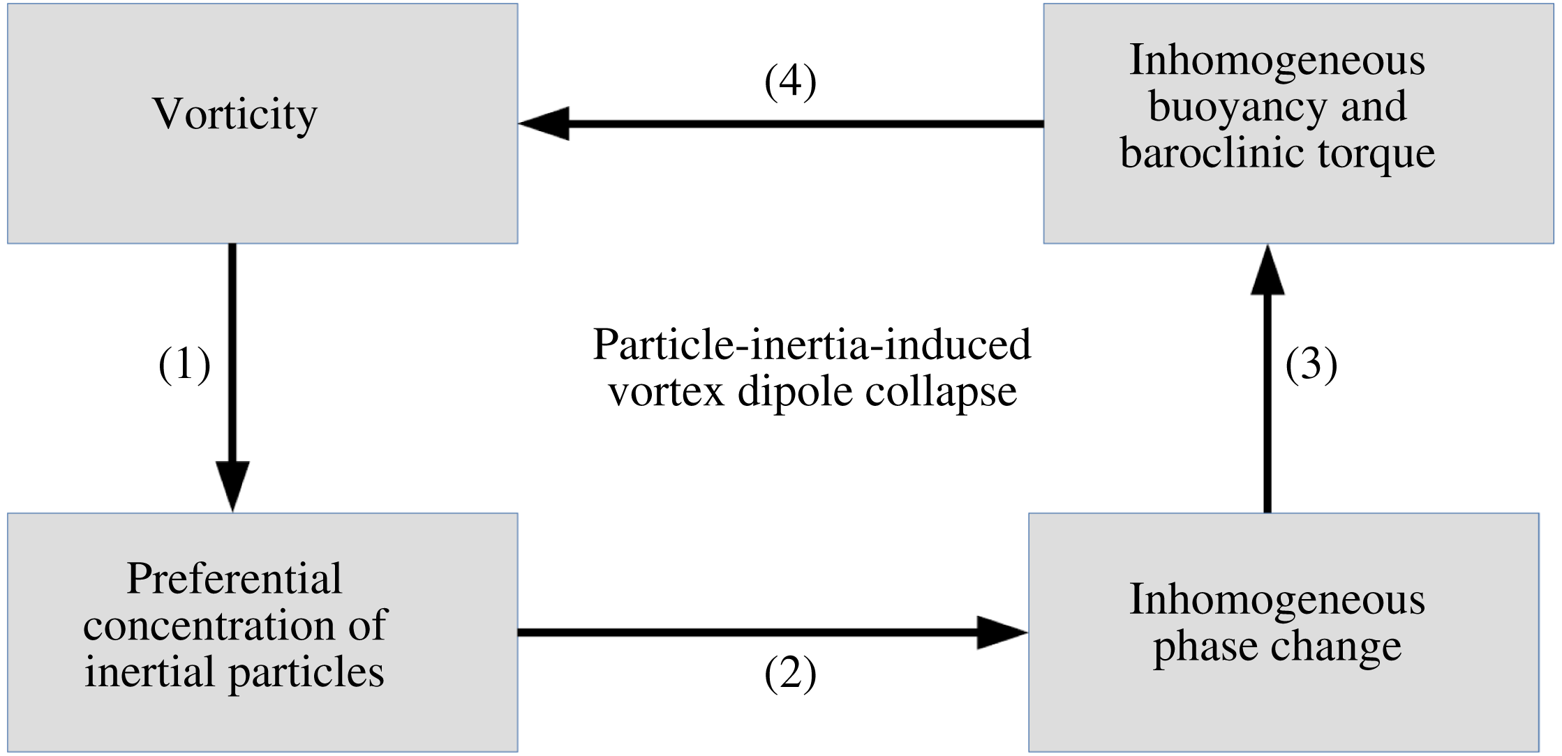
A fundamental problem of cloud physics is to link the dynamics at the small scales (the behaviour of water droplets, say) to the dynamics at the large scale (the dynamics of coherent vortices). One possible route is sketched in the schematic below (figure 1, modified from Narasimha et al. (Reference Narasimha, Diwan, Duvvuri, Sreenivas and Bhat2011)), and provides an idea of the interactions in a cloud-like flow as follows. We know that water droplets in clouds behave like Stokesian particles – particles that experience a drag proportional to the slip velocity between them and the fluid. This means that droplets are expelled from regions of high vorticity (see, e.g. Shaw et al. Reference Shaw, Reade, Collins and Verlinde1998; Ravichandran & Govindarajan Reference Ravichandran and Govindarajan2015). This provides link (1) in the schematic between vorticity and particle inertia. Water droplets in clouds are formed by the activation of aerosol particles. They act as the nuclei for the condensation of water vapour. They grow by the condensation of water vapour onto their surfaces, releasing latent heat in the process. The rate at which the droplets grow is inversely proportional to their current size, making this process highly nonlinear. This provides link (2) in the schematic. Water droplets, being inertial particles, are not uniformly distributed over the flow. As these water droplets grow by condensation, latent heat is released only in regions that have water droplets. This differential heating, in the presence of gravity, leads to different regions in the flow experiencing different buoyancy forces, providing link (3). The baroclinic torque that is thus created then acts on the vorticity in the flow, in link (4), completing the loop.
Schematic of the interactions that determine a cloud flow. Labelled against the particular interaction are the mechanisms that arise in this study: (1) inertial particles are expelled from vortical regions; (2) phase change takes place only in regions with particles; (3) buoyancy acts selectively in regions where phase change occurs; (4) differential buoyancy results in baroclinic torque and, thus, production of small-scale vorticity.

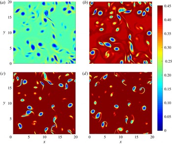
In this paper, we study a model fluid mechanical problem that has all these mechanisms in action. First, we show that two identical counter-signed vortices expel inertial droplets from their vicinity. This creates a dearth of condensation nuclei in this region, so condensation takes place preferentially outside this region. A temperature differential follows, and buoyancy radically alters the vortex dynamics. The last part of this process consists of a complete collapse of the vortex dipole, similar to that demonstrated in a recent study by Ravichandran et al. (Reference Ravichandran, Dixit and Govindarajan2017). It is caused due to the action of a Magnus lift force, provided the vortices in the dipole have density patches coincident with them. We then show, in simulations with many vortices, that this interaction of the time scales of particle inertia and phase change causes a transfer of kinetic energy and enstrophy to the small scales.
In § 2, we describe the physics of the system in terms of the various non-dimensional parameters governing it. In § 3, we describe the method of, and perform, numerical simulations of the system. We show how the collapse of the vortex dipole occurs as a result of the various forces at play. In § 4, we provide some theoretical arguments to account for the behaviour displayed in our simulations, and for when these mechanisms will not apply. We conclude in § 5, with some thoughts on future directions.
2 Problem set-up
We treat the mixture of dry air and water vapour and liquid water components to be a single fluid (moist air) with constant properties of kinematic viscosity
 $\unicode[STIX]{x1D708}$
and heat capacity
 $C_{p}$
. To highlight the physics we consider the simplest geometry, of a pair of opposite-signed Gaussian vortices, each of maximum vorticity magnitude
 $\unicode[STIX]{x1D6FA}_{0}$
and characteristic diameter
 $d_{0}$
(
 $\unicode[STIX]{x1D714}(r)=\unicode[STIX]{x1D6FA}_{0}\exp (-4r^{2}/d_{0}^{2})$
in cylindrical coordinates) in two dimensions, in a gravitational field of strength
 $g(-\hat{\boldsymbol{e}}_{y})$
, where
 $y$
is the vertical coordinate. Towards the end of the paper we will extend our study to a more general flow. The environment that we place these vortices in is described in the succeeding subsections. The Reynolds and Froude numbers are defined by
 $$\begin{eqnarray}\displaystyle \left.\begin{array}{@{}c@{}}\displaystyle Re,\text{the Reynolds number},=\frac{\unicode[STIX]{x1D6FA}_{0}d_{0}^{2}}{\unicode[STIX]{x1D708}},\\ \displaystyle Fr^{2},\text{the Froude number},=\frac{\unicode[STIX]{x1D6FA}_{0}^{2}d_{0}}{gA},\end{array}\right\} & & \displaystyle\end{eqnarray}$$
where the Atwood number,
 $A=\unicode[STIX]{x0394}T/T_{0}$
, gives the magnitude of characteristic density changes in the flow. Since the problem involves thermodynamics and phase change, the Atwood number is in fact a function of time, parametrised by the enthalpy of vaporisation
 $L_{v}$
, and the gas constant for pure water vapour
 $R_{v}$
(through the Clausius–Clapeyron equation for the saturation vapour pressure, equation (2.3)).
2.1 Thermodynamics
Our system involves the condensation of supersaturated water vapour on to small droplets of water (or aerosol particles to start with). A droplet bigger than the Kohler critical radius (Bohren & Albrecht Reference Bohren and Albrecht2000, chapter 7) grows by water vapour in the supersaturated surroundings diffusing towards the droplet and condensing onto its surface. The energy that is released in this process diffuses outwards from the surface of the droplet. This gives, for the rate of growth of the droplet of radius
 $a$
,
 $$\begin{eqnarray}a\frac{\text{d}a}{\text{d}t}=\frac{1}{C\unicode[STIX]{x1D70C}_{w}}\left(\frac{r_{v}}{r_{s}}-1\right),\end{eqnarray}$$
where
 $C$
is a weak function of temperature, with a value for water, in SI units, of
 $10^{7}~\text{m}~\text{s}~\text{kg}^{-1}$
,
 $\unicode[STIX]{x1D70C}_{w}$
is the density of liquid water, which can be taken to be
 $1000~\text{kg}~\text{m}^{-3}$
. For convenience, we use mixing ratios for defining concentrations of water vapour and liquid water: a mixing ratio is the mass of water substance present per unit mass of dry air. The mixing ratios
 $r_{v}$
,
 $r_{s}$
and
 $r_{l}$
, for water vapour, saturated vapour and liquid water, respectively, are therefore defined as
 $r_{v,s,l}=\unicode[STIX]{x1D70C}_{v,s,l}/\unicode[STIX]{x1D70C}_{0}$
, where
 $\unicode[STIX]{x1D70C}_{v}$
is the mass of water vapour per unit volume of the system,
 $\unicode[STIX]{x1D70C}_{s}$
is the mass of vapour in a saturated unit volume,
 $\unicode[STIX]{x1D70C}_{l}$
is the mass of liquid water in this volume, and
 $\unicode[STIX]{x1D70C}_{0}$
is the density of dry air. The saturation mixing ratio
 $r_{s}$
is given as a function of the temperature
 $T$
by the Clausius–Clapeyron equation
 $$\begin{eqnarray}r_{s}=r_{s}^{0}\exp \left[\frac{L_{v}}{R_{v}}\left\{\frac{1}{T_{0}}-\frac{1}{T}\right\}\right],\end{eqnarray}$$
where
 $T_{0}$
is some base (absolute) temperature, and
 $r_{s}^{0}$
is the saturation vapour mixing ratio at
 $T_{0}$
. Note that the saturation vapour mixing ratio is technically also a function of the ambient pressure, but to simplify the problem we assume that the ambient pressure is constant.
We treat the droplets as forming a field, so (2.2) may be used to write, for the rate of change of the liquid mixing ratio,
 $$\begin{eqnarray}\frac{\text{d}r_{l}}{\text{d}t}=n\left[4\unicode[STIX]{x03C0}a^{2}\frac{\text{d}a}{\text{d}t}\right]\frac{\unicode[STIX]{x1D70C}_{w}}{\unicode[STIX]{x1D70C}_{0}},\end{eqnarray}$$
where
 $n$
is the number of droplets per unit volume. Substituting for the rate of growth of the droplet radius from (2.2) gives
 $$\begin{eqnarray}\frac{\text{d}r_{l}}{\text{d}t}=\left[\frac{4\unicode[STIX]{x03C0}an}{C}\right]\left[\frac{r_{v}}{r_{s}}-1\right].\end{eqnarray}$$
Similar equations for the evolution of the particle size and liquid water have been used in Shaw et al. (Reference Shaw, Reade, Collins and Verlinde1998), Kumar, Schumacher & Shaw (Reference Kumar, Schumacher and Shaw2013) and de Lozar & Mellado (Reference de Lozar and Mellado2014). We will find it convenient to express the water-substance-related quantities normalised by
 $r_{s}^{0}$
, and to express the temperature
 $T$
as a deviation from the base temperature
 $T_{0}$
:
 $$\begin{eqnarray}T=T_{0}+\unicode[STIX]{x1D703}\unicode[STIX]{x0394}T.\end{eqnarray}$$
Here,
 $\unicode[STIX]{x0394}T$
is a scale for temperature variations, and is typically much smaller than the absolute temperature
 $T_{0}$
. The variable
 $\unicode[STIX]{x1D703}$
is
 $O(1)$
by this definition. Assuming the Atwood number
 $A=\unicode[STIX]{x0394}T/T_{0}\ll 1$
, the normalised Clausius–Clapeyron equation can be written approximately as
 $$\begin{eqnarray}r_{s}=\exp \left[\frac{L_{v}\unicode[STIX]{x0394}T}{R_{v}T_{0}^{2}}\unicode[STIX]{x1D703}\right],\end{eqnarray}$$
where
 $L_{v}\unicode[STIX]{x0394}T/R_{v}T_{0}^{2}$
is a dimensionless constant. The normalised condensation equation (2.5) then becomes
 $$\begin{eqnarray}\frac{\text{d}r_{l}}{\text{d}t}=\frac{{\mathcal{H}}}{\unicode[STIX]{x1D70F}_{s}}\left[\frac{r_{v}}{r_{s}}-1\right],\end{eqnarray}$$
which also defines
 $\unicode[STIX]{x1D70F}_{s}$
, the time scale for phase change as
 $$\begin{eqnarray}\unicode[STIX]{x1D70F}_{s}\equiv \frac{Cr_{s}^{0}}{4\unicode[STIX]{x03C0}an}.\end{eqnarray}$$
The time scale for phase change thus depends on the saturation mixing ratio
 $r_{s}^{0}$
, and on the number density of water droplets
 $n$
. In the atmosphere, both these quantities typically fall steeply with height (the former because of its sensitive dependence on the base temperature
 $T_{0}$
). In calculating realistic non-dimensional parameters we use values of these representative of altitudes lower than clouds, but expect that the ratio maintains the same order of magnitude.
The factor
 ${\mathcal{H}}$
takes into account the fact that liquid mixing ratio cannot go below
 $0$
, so we cannot have evaporation unless there is liquid.
 $$\begin{eqnarray}{\mathcal{H}}=\left\{\begin{array}{@{}ll@{}}1,\quad & r_{v}\geqslant r_{s},\\ 1,\quad & r_{v}<r_{s},r_{l}>0,\\ 0,\quad & r_{v}<r_{s},r_{l}=0.\end{array}\right.\end{eqnarray}$$
The vapour and liquid production terms are negatives of each other; each unit of vapour that condenses adds energy to the amount of
 $L_{v}$
to the fluid of heat capacity
 $C_{p}$
. The equations for vapour and temperature are, therefore,
 $$\begin{eqnarray}\displaystyle & \displaystyle \frac{\text{d}r_{v}}{\text{d}t}=-\frac{{\mathcal{H}}}{\unicode[STIX]{x1D70F}_{s}}\left[\frac{r_{v}}{r_{s}}-1\right], & \displaystyle\end{eqnarray}$$
 $$\begin{eqnarray}\displaystyle & \displaystyle \frac{\text{d}\unicode[STIX]{x1D703}}{\text{d}t}=\left[\frac{L_{v}}{C_{p}\unicode[STIX]{x0394}T}\right]\frac{{\mathcal{H}}}{\unicode[STIX]{x1D70F}_{s}}\left[\frac{r_{v}}{r_{s}}-1\right]. & \displaystyle\end{eqnarray}$$
Equations (2.8) and (2.12) imply that the following quantities are conserved:
 $$\begin{eqnarray}\displaystyle \left.\begin{array}{@{}c@{}}\displaystyle \text{the moist enthalpy }H_{moist}=\unicode[STIX]{x1D703}+\frac{L_{v}r_{s}^{0}}{C_{p}\unicode[STIX]{x0394}T}r_{v},\\ \displaystyle \text{the dry enthalpy }H_{dry}=\unicode[STIX]{x1D703}-\frac{L_{v}r_{s}^{0}}{C_{p}\unicode[STIX]{x0394}T}r_{l},\\ \displaystyle \text{the total water content }r_{t}=r_{v}+r_{l}.\end{array}\right\} & & \displaystyle\end{eqnarray}$$
2.2 Particle inertia
The equation of motion of a single (spherical) droplet in fluid flow is given by the Maxey–Riley equations of motion (Maxey & Riley Reference Maxey and Riley1983). For small heavy particles, these equations simplify greatly to give, for the motion of a single droplet with a Stokes time lag of
 $\unicode[STIX]{x1D70F}_{p}$
,
 $$\begin{eqnarray}\frac{\text{d}\boldsymbol{v}}{\text{d}t}=\frac{\boldsymbol{u}-\boldsymbol{v}}{\unicode[STIX]{x1D70F}_{p}}+\unicode[STIX]{x1D70F}_{p}\boldsymbol{g},\end{eqnarray}$$
where
 $\boldsymbol{v}$
is the velocity of the droplet and
 $\boldsymbol{u}$
is the velocity of the fluid at the location of the centre of the droplet. In our studies here, we ignore the gravity-driven settling term on the right-hand side. That is, we assume that the liquid droplets formed do not settle appreciably during the time of our interest, i.e. that
 $\unicode[STIX]{x1D70F}_{p}g/|\boldsymbol{v}|\approx \unicode[STIX]{x1D70F}_{p}g/|\boldsymbol{u}|=\unicode[STIX]{x1D70F}_{p}g/\unicode[STIX]{x1D6FA}_{0}d_{0}\ll 1$
. Note, however, that the gravity term is not necessarily small compared to the fluid acceleration term:
 $\unicode[STIX]{x1D70F}_{p}g/\unicode[STIX]{x1D70F}_{p}|\text{D}u/\text{D}t|=g/\unicode[STIX]{x1D6FA}_{0}^{2}d_{0}=1/(Fr^{2}A)$
. We return to this point in § 4.4.
Non-dimensionalising using
 $\unicode[STIX]{x1D6FA}_{0}$
and
 $d_{0}$
, and defining the particle Stokes number as
 $St_{p}\equiv \unicode[STIX]{x1D6FA}_{0}\unicode[STIX]{x1D70F}_{p}$
, we have
 $$\begin{eqnarray}\frac{\text{d}\boldsymbol{v}}{\text{d}t}=\frac{\boldsymbol{u}-\boldsymbol{v}}{St_{p}}.\end{eqnarray}$$
Equation (2.15) admits solutions for
 $\boldsymbol{v}$
which do not comprise a field (see, e.g. Ravichandran & Govindarajan Reference Ravichandran and Govindarajan2015). It is thus suitable for Eulerian–Lagrangian simulations where each droplet is tracked, but cannot be used in our treatment of droplets as a field. For small Stokes number, we may derive an approximation to this equation as follows.
 $$\begin{eqnarray}\boldsymbol{v}=\boldsymbol{u}-St_{p}\frac{\text{d}\boldsymbol{v}}{\text{d}t}=\boldsymbol{u}-St_{p}\frac{\text{D}\boldsymbol{u}}{\text{D}t}+O(St_{p}^{2}).\end{eqnarray}$$
Equation (2.16) is correct to
 $O(St_{p})$
, and is sometimes called the ‘inertial equation’. This form of the equation for droplet velocity, we note, now describes a field. We work with this approximation, and point out some consequences of making this approximation in appendix A. This approach has been used earlier, e.g. by de Lozar & Mellado (Reference de Lozar and Mellado2014).
The liquid mixing ratio
 $r_{l}$
is advected with this velocity
 $\boldsymbol{v}$
instead of the fluid velocity
 $\boldsymbol{u}$
. The droplet velocity field, unlike the fluid velocity field, is not incompressible. The advection equation for the liquid can therefore be written as
 $$\begin{eqnarray}\frac{\unicode[STIX]{x2202}r_{l}}{\unicode[STIX]{x2202}t}+\unicode[STIX]{x1D735}\boldsymbol{\cdot }(\boldsymbol{v}r_{l})=0.\end{eqnarray}$$
2.3 Governing equations
We work in two space dimensions, and write the Navier–Stokes equations in streamfunction–vorticity
 $(\unicode[STIX]{x1D713}{-}\unicode[STIX]{x1D714})$
variables. The equations for the scalars below combine the contributions from the thermodynamics and particle inertia discussed above, apart from diffusion. The non-dimensional equations are
 $$\begin{eqnarray}\displaystyle \left.\begin{array}{@{}c@{}}\displaystyle \frac{\unicode[STIX]{x2202}\unicode[STIX]{x1D714}}{\unicode[STIX]{x2202}t}+\boldsymbol{u}\boldsymbol{\cdot }\unicode[STIX]{x1D735}\unicode[STIX]{x1D714}=\frac{1}{Re}\unicode[STIX]{x1D6FB}^{2}\unicode[STIX]{x1D714}+\frac{\unicode[STIX]{x2202}B}{\unicode[STIX]{x2202}x},\\ \displaystyle \frac{\unicode[STIX]{x2202}\unicode[STIX]{x1D703}}{\unicode[STIX]{x2202}t}+\boldsymbol{u}\boldsymbol{\cdot }\unicode[STIX]{x1D735}\unicode[STIX]{x1D703}=\frac{1}{RePr_{\unicode[STIX]{x1D703}}}\unicode[STIX]{x1D6FB}^{2}\unicode[STIX]{x1D703}+{\mathcal{H}}\frac{L_{v}r_{s}^{0}}{C_{p}\unicode[STIX]{x0394}T}\left(\frac{r_{v}-r_{s}}{r_{s}St_{s}}\right),\\ \displaystyle \frac{\unicode[STIX]{x2202}r_{v}}{\unicode[STIX]{x2202}t}+\boldsymbol{u}\boldsymbol{\cdot }\unicode[STIX]{x1D735}r_{v}=\frac{1}{RePr_{v}}\unicode[STIX]{x1D6FB}^{2}r_{v}-{\mathcal{H}}\left(\frac{r_{v}-r_{s}}{r_{s}St_{s}}\right),\\ \displaystyle \frac{\unicode[STIX]{x2202}r_{l}}{\unicode[STIX]{x2202}t}+\unicode[STIX]{x1D735}\boldsymbol{\cdot }(\boldsymbol{v}r_{l})=\frac{1}{RePr_{l}}\unicode[STIX]{x1D6FB}^{2}r_{l}+{\mathcal{H}}\left(\frac{r_{v}-r_{s}}{r_{s}St_{s}}\right),\end{array}\right\} & & \displaystyle\end{eqnarray}$$
where
 $B$
is the buoyancy, and
 $Pr_{\unicode[STIX]{x1D703},r_{v},r_{l}}$
are the Prandtl numbers associated with the different scalars. The Stokes number for phase change,
 $St_{s}\equiv \unicode[STIX]{x1D6FA}_{0}\unicode[STIX]{x1D70F}_{s}$
, with
 $\unicode[STIX]{x1D70F}_{s}$
given in (2.9). The first of equations (2.18) is the Boussinesq vorticity equation in two dimensions, and contains the baroclinic torque term. The second is the temperature equation, in which the last term is a source due to phase change. The third and fourth equations are the evolution equations for vapour and liquid phases of water, and include the phase-change term with the appropriate sign. The quantity
 ${\mathcal{H}}$
, defined in (2.10), avoids unphysical phase change. Note that both condensation and evaporation require the presence of liquid, the latter for obvious reasons and the former because liquid acts as a nucleation site for condensation. It is well known that in the absence of liquid or solid surfaces, supersaturation levels need to be unrealistically high for spontaneous condensation without nucleation sites to occur. The liquid is measured here in units of
 $n$
, the number of identical droplets. As
 $r_{l}$
goes down,
 $n$
goes down, and the phase-change time goes to infinity. The fluid velocity components are given by
 $$\begin{eqnarray}u=\boldsymbol{u}\boldsymbol{\cdot }\hat{\boldsymbol{e}}_{x}=\frac{\unicode[STIX]{x2202}\unicode[STIX]{x1D713}}{\unicode[STIX]{x2202}y};\quad v=\boldsymbol{u}\boldsymbol{\cdot }\hat{\boldsymbol{e}}_{y}=-\frac{\unicode[STIX]{x2202}\unicode[STIX]{x1D713}}{\unicode[STIX]{x2202}x},\end{eqnarray}$$
and the streamfunction is given by solving the Poisson equation
 $$\begin{eqnarray}\unicode[STIX]{x1D6FB}^{2}\unicode[STIX]{x1D713}=-\unicode[STIX]{x1D714}.\end{eqnarray}$$
The buoyancy
 $B$
is in general a combination of the temperature
 $\unicode[STIX]{x1D703}$
, and the vapour and liquid mixing ratios
 $r_{v}$
and
 $r_{l}$
. However, in most Eulerian–Lagrangian studies where individual particles are tracked, a one-way coupling – the fluid transfers momentum to the particle, but not the reverse – is assumed. Bosse, Kleiser & Meiburg (Reference Bosse, Kleiser and Meiburg2006) find that this approximation becomes invalid when the volume fraction of the liquid droplets is larger than approximately
 $10^{-5}$
. Since the volume fraction of liquid droplets in our scenario (given by
 $\unicode[STIX]{x1D719}\sim na^{3}$
) is much smaller, we may justifiably use this approximation. This amounts to dropping the buoyancy contribution of liquid water; for simplicity, and since it is a good approximation, we also drop the buoyancy contribution of water vapour, leaving, for the buoyancy,
 $$\begin{eqnarray}\boldsymbol{B}=\frac{\unicode[STIX]{x1D703}}{Fr^{2}}\hat{\boldsymbol{e}}_{y}.\end{eqnarray}$$
The maximum difference in vapour mixing ratios in the flow is proportional to the supersaturation, and the total amount of liquid is small. As a result, the magnitude of the buoyancy induced by the water components is
 $O(10^{-2})$
of the buoyancy due to temperature changes induced by the phase change.
As the system evolves from its uniform supersaturated initial state, on an average
 $r_{l}$
increases at the expense of
 $r_{v}$
. For simplicity we assume that particle inertia
 $St_{p}$
remains constant, i.e. that condensation results in the formation of new droplets, which are all of the same size. In reality, for conditions typical of clouds, the average
 $St_{p}$
would undergo a slow increase, since
 $St_{s}\gg 1$
(see § 4.4) on a time scale proportional to the phase-change time scale
 $\unicode[STIX]{x1D70F}_{s}$
. Typically it will double in our entire simulation time and so is not expected to change the effect on buoyancy. We have made this approximation for simplicity, but not making it will enhance our mechanism, since this assumption underestimates the effective phase-change Stokes number. This approximation allows us to express the phase-change time scale
 $\unicode[STIX]{x1D70F}_{s}$
, from (2.9), as simply being inversely proportional to the liquid mixing ratio:
 $$\begin{eqnarray}\unicode[STIX]{x1D70F}_{s}=\frac{\unicode[STIX]{x1D70F}_{s}(t=0)r_{l}(t=0)}{r_{l}}.\end{eqnarray}$$
2.4 Lift-induced vortex-dipole collapse
The mechanism of vortex dipoles collapsing under the action of a Kutta lift was discussed in Ravichandran et al. (Reference Ravichandran, Dixit and Govindarajan2017). It was shown that buoyant vortices behave much like spinning cylinders, experiencing a velocity relative to the fluid around them and a concomitant lift force. In a simple model the lift on a vortex of strength
 $\unicode[STIX]{x1D71E}$
is
 ${\sim}\unicode[STIX]{x1D70C}_{0}\unicode[STIX]{x1D71E}\times \boldsymbol{w}$
, where
 $\boldsymbol{w}$
is the velocity of the vortex relative to the fluid. The following equation of motion was shown to accurately describe the motion of the vortices while they are not significantly distorted from a circular shape:
 $$\begin{eqnarray}\frac{\text{d}\boldsymbol{w}}{\text{d}t}=\frac{Fr^{-2}}{1-A}\hat{\boldsymbol{e}}_{y}+\frac{\hat{\boldsymbol{e}}_{z}\times \boldsymbol{w}}{1-A}.\end{eqnarray}$$
The lift force, appearing as the second term on the right-hand side in (2.23), is perpendicular to both the axis of the vortex and to the relative velocity
 $\boldsymbol{w}$
. If two such oppositely signed vortices are placed next to each other with the right orientation, the lift force will propel them at each other.
2.5 Parameter space and simulation details
The vortices are initially in a uniform ambient, with
 $\unicode[STIX]{x1D703}=0$
and
 $r_{v}$
and
 $r_{l}$
constant over space. Except when we study the effect of the initial supersaturation value in § 3.3, we set the initial values of
 $r_{v}(t=0)=1.04$
, amounting to a supersaturation of 4 %; and
 $r_{l}(t=0)=0.001$
.
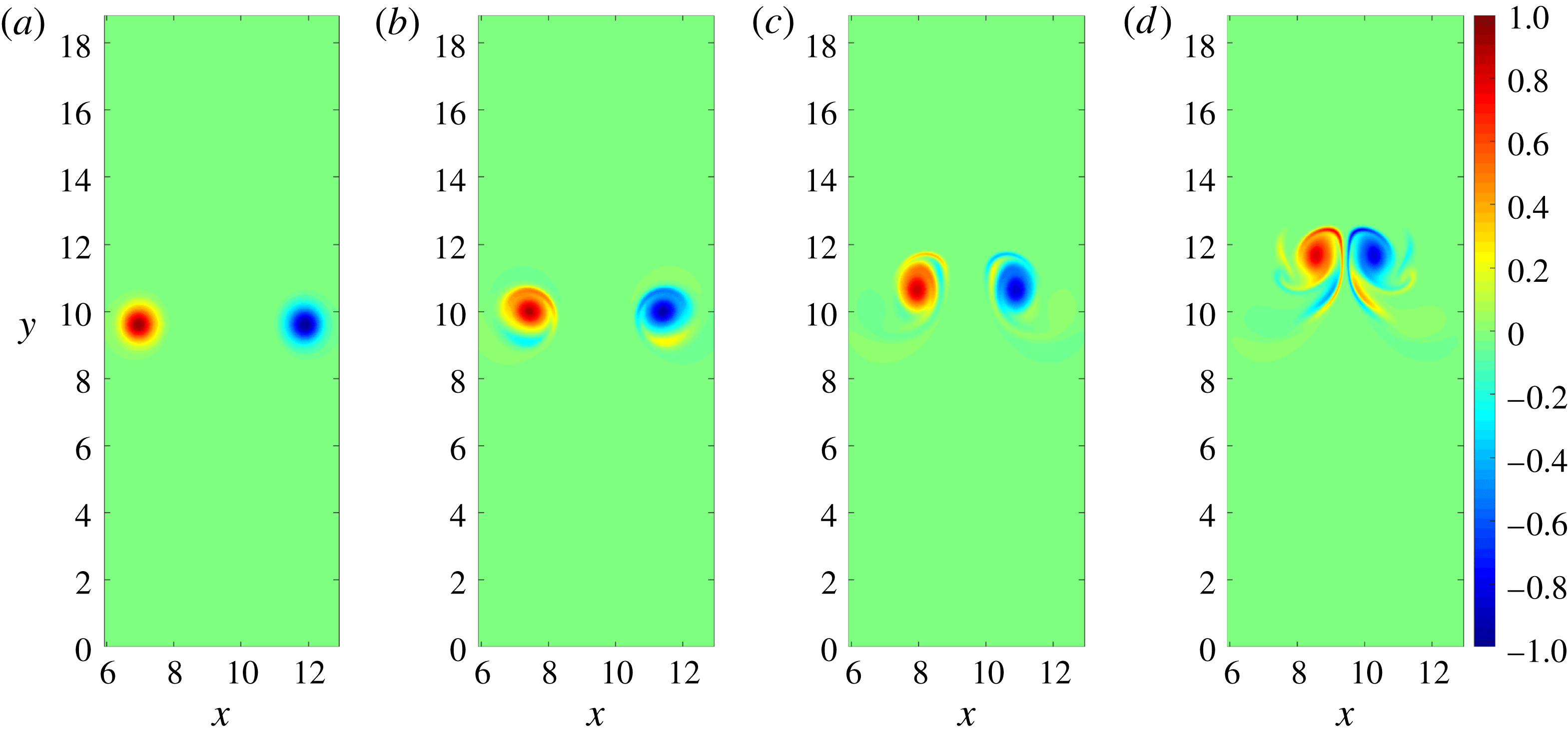
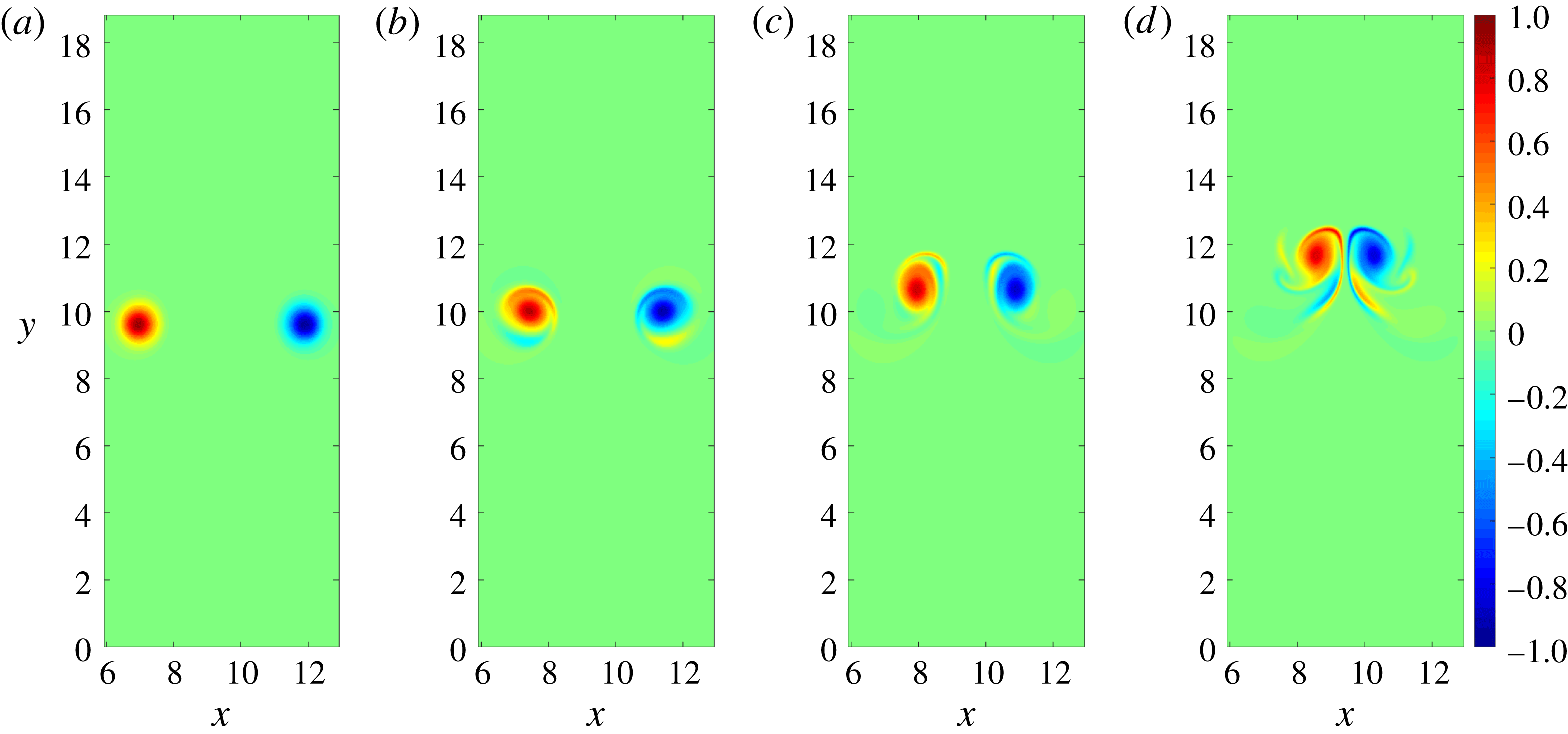
Positions of the vortices (left: positive-signed, right: negative-signed) at early times, for the case
 $St_{p}=1$
,
 $St_{s}=200$
. The vortices are shown at
 $t=10,30,50,70$
(a–d, respectively). Due to their mutual induced velocities they move slowly vertically upwards, but they are also seen to move closer to each other and begin to distort from their circular shape.
The parameter space of the problem consists of four numbers:
 $Re,Fr^{2},St_{s},St_{p}$
, in addition to initial supersaturation, the initial horizontal separation between the vortices, and the Prandtl numbers for the temperature and water components. Except when we explicitly discuss the effects of supersaturation in § 3.3, we keep the initial supersaturation fixed at
 $s_{0}=1.04$
, and the initial
 $r_{l}=0.001$
. The other relevant parameters are:
 $r_{s}^{0}=0.02$
at
 $T_{0}=290~\text{K}$
, giving
 $L_{v}r_{s}^{0}/(C_{p}\unicode[STIX]{x0394}T)=48$
. The Prandtl numbers are
 $Pr_{\unicode[STIX]{x1D703}}=Pr_{v}=1$
, and
 $Pr_{l}=\infty$
. We keep the initial horizontal separation (in units of the vortex diameter) between the vortices fixed at
 $\unicode[STIX]{x0394}x_{(t=0)}=5$
, and the box size fixed at
 $6\unicode[STIX]{x03C0}\times 6\unicode[STIX]{x03C0}$
. The vortices are initially located on a line perpendicular to the direction of gravity, as seen in figure 2. Lastly, we assume that the temperature and vapour have the same Prandtl number of unity, and assume that the liquid component does not diffuse
 $(Pr_{l}=\infty )$
. The effects of varying the Reynolds and Froude numbers, and the horizontal separation of the vortices, were considered at length by Ravichandran et al. (Reference Ravichandran, Dixit and Govindarajan2017). That study began with light or heavy vortices and did not include thermodynamics, but since we expect the effect of varying those parameters to be qualitatively the same in the present flow as well, we do not repeat that exercise.
In the range of Reynolds and Froude numbers we will consider here, the lift force that drives the dynamics of interest is independent of the Reynolds number and inversely proportional to
 $Fr^{2}$
, such that (2.23) approximates the dynamics of motion of the vortices when they are undistorted. Our main focus here is the thermodynamics, and the non-dimensional numbers of primary importance to us are
 $St_{s}$
and
 $St_{p}$
. Besides these, the initial supersaturation is an additional parameter, and we will return to it later.
We perform numerical simulations of (2.18) in a periodic box. We use a Fourier-pseudospectral method for the vorticity, vapour, and temperature equations to convert the partial differential equations into algebraic equations in time, and use the
 $2/3$
dealiasing rule to avoid aliasing errors. Simulations involving the thermodynamics of phase change, especially given the highly nonlinear nature of the Clausius–Clapeyron equation, are known to suffer if negative liquid values could arise. We therefore use a first-order upwind scheme for the liquid equation, ensuring that no negative liquid can arise. The time integration is done using a third-order strong-stability-preserving Runge–Kutta (SSPRK, see Gottlieb, Shu & Tadmor (Reference Gottlieb, Shu and Tadmor2001)) for the nonlinear terms; the linear (viscous) terms are handled implicitly using a Crank Nicolson scheme. The code has been validated against results from Ravichandran et al. (Reference Ravichandran, Dixit and Govindarajan2017). Unless otherwise mentioned, we use
 $1024^{2}$
Fourier modes for our simulations.
3 Results
In our numerical simulations we impose a uniform initial liquid concentration corresponding to a number density of
 $O(10^{7})$
droplets of
 $10~\unicode[STIX]{x03BC}\text{m}$
radius per
 $\text{m}^{3}$
. We first discuss in some detail the particular case of Stokes numbers
 $St_{p}=1$
and initial
 $St_{s}=200$
. Other parameters are initialised as detailed in § 2.5. This case is a standard example of how phase change can affect the dynamics.
At
 $t=0$
, the vortices are placed in the middle of the box (
 $y=3\unicode[STIX]{x03C0}$
), and their positions at moderate times
 $t$
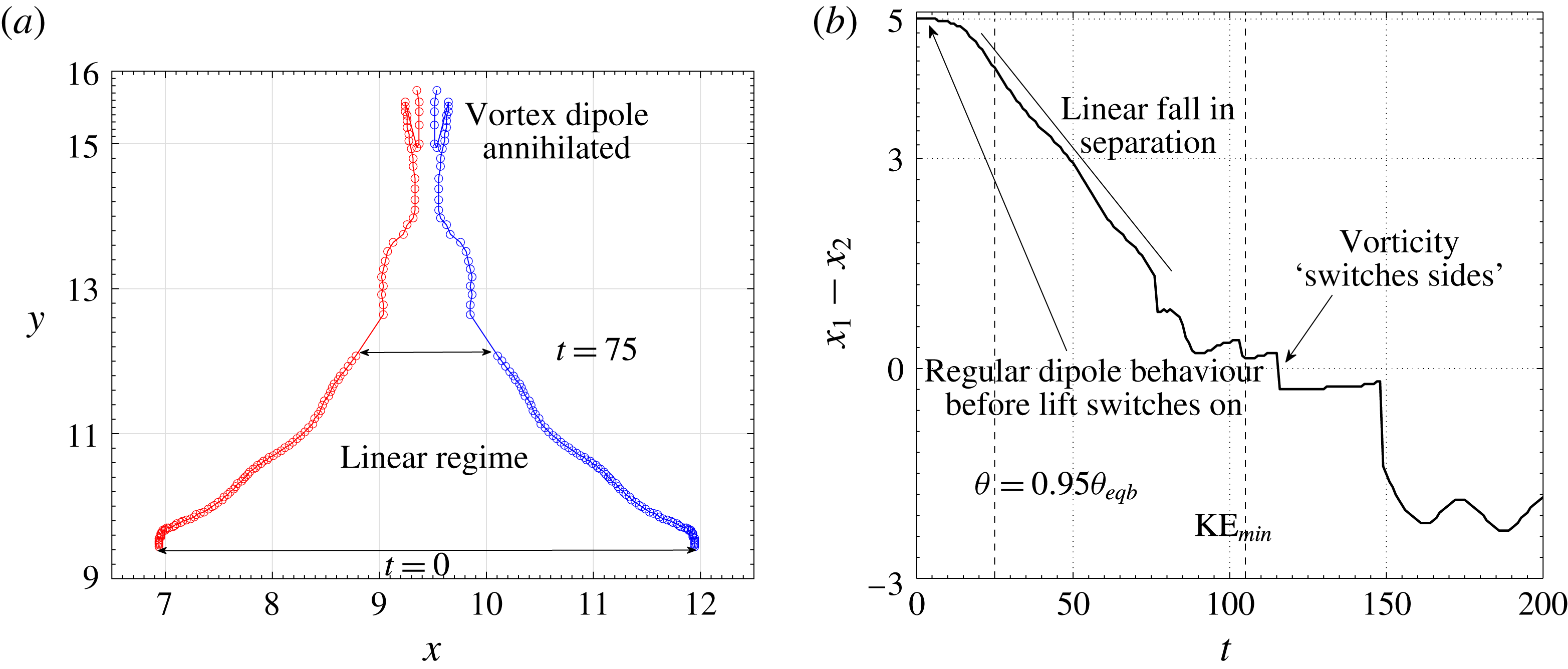
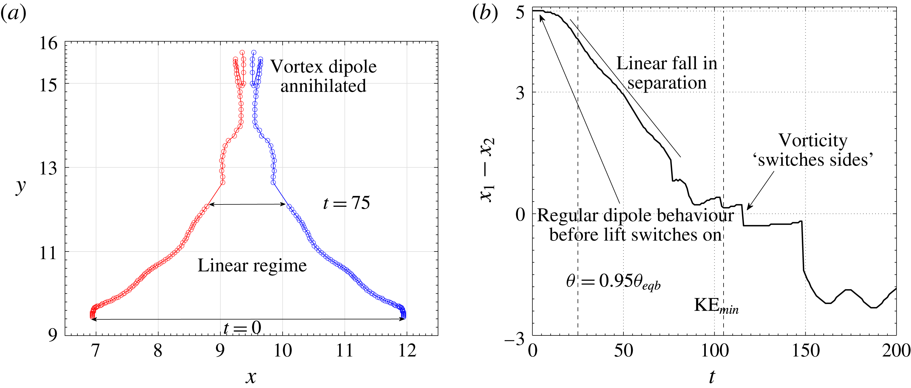
can be seen in figure 2. Note that the vortices remain approximately circular during the initial stage. The complete trajectories of the vortices, obtained by plotting the vorticity maxima of either sign, are shown in figure 3. On the right of the same figure, the horizontal separation between them is shown as a function of time. The motion of the vortices occurs in three regimes.
For
 $t\lesssim 5$
, the vortices move vertically upwards, maintaining the horizontal separation between them. It will be seen below that no significant phase change has occurred before this time. Thereafter, following a brief adjustment period, the horizontal separation between the vortices falls linearly between
 $t\approx 10$
and
 $t\approx 80$
, at which time the vortices are annihilated. This linear fall in the separation occurs because of the constant lateral velocities induced on the now buoyant vortices by the lift force acting on them. As the separation goes to zero, the original vortices get annihilated. Thereafter the horizontal separation becomes negative, which we shall see below to be because of the counter-signed vorticity produced by the tails of low temperature left behind by the vortices. We discuss the lift-driven linear regime first, before discussing the dynamics of vorticity annihilation.
(a) Trajectories of the oppositely signed vortices. The vortices are tracked by locating the maximum and minimum vorticities in the box. This procedure fails when the parent vortices are annihilated. The case shown has
 $St_{s}=200$
,
 $St_{p}=1$
. The circles are drawn at intervals of
 $\unicode[STIX]{x0394}t=1$
. (b) The horizontal separation between the vortices, showing different regimes of motion: the initial regime where the vortices behave like a standard dipole; the final regime where the vortices behave like the buoyant dipole of Ravichandran et al. (Reference Ravichandran, Dixit and Govindarajan2017); and the short-lived intermediate regime where the system transitions between these two limiting behaviours.
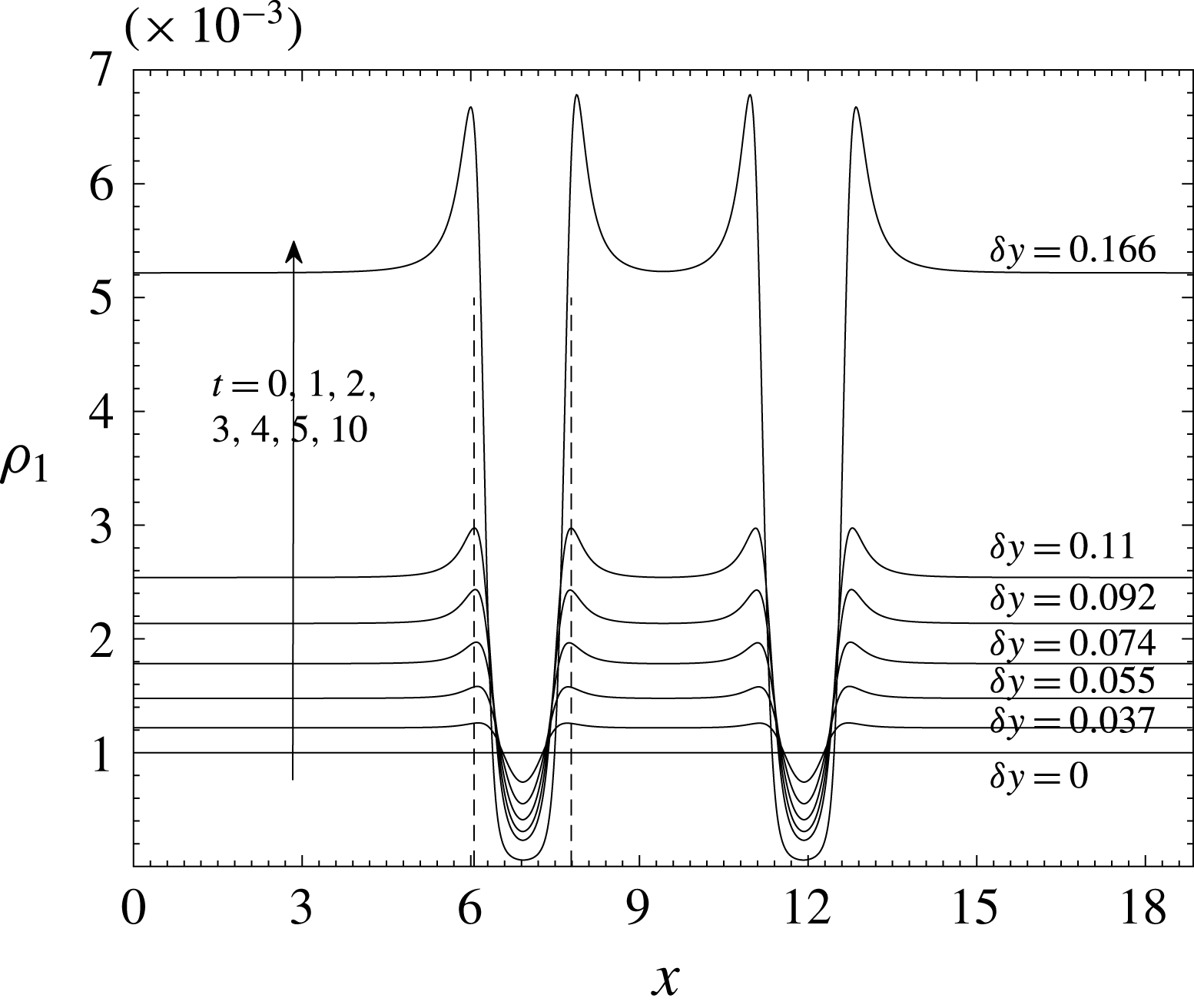
Radial profiles of liquid concentration at early times (indicated next to each curve). Also shown in the figure are the corresponding vertical displacements of the vortex pair from the initial vertical location of the vortex dipole. The size of the region with no liquid grows slowly with time, and the minimum liquid mixing ratio keeps falling.

Horizontal profiles of the temperature
 $\unicode[STIX]{x1D703}$
(a) and the vapour mixing ratio
 $r_{v}$
(b) in the initial stages of evolution for the case
 $St_{s}=200$
,
 $St_{p}=1$
. At each time, the vertical location
 $y$
is chosen to be coincident with that of the vortex centroids. Clearly seen are the (colder and vapour-rich) voids formed because of particle inertia. Also seen, because of the accumulation of the droplets around the vortices in ‘halos’, are higher temperatures regions around the vortices. The profiles, as expected, are symmetric about the horizontal centre (
 $x=3\unicode[STIX]{x03C0}$
). The vertical dotted lines are drawn at the horizontal locations of the ‘halos’.

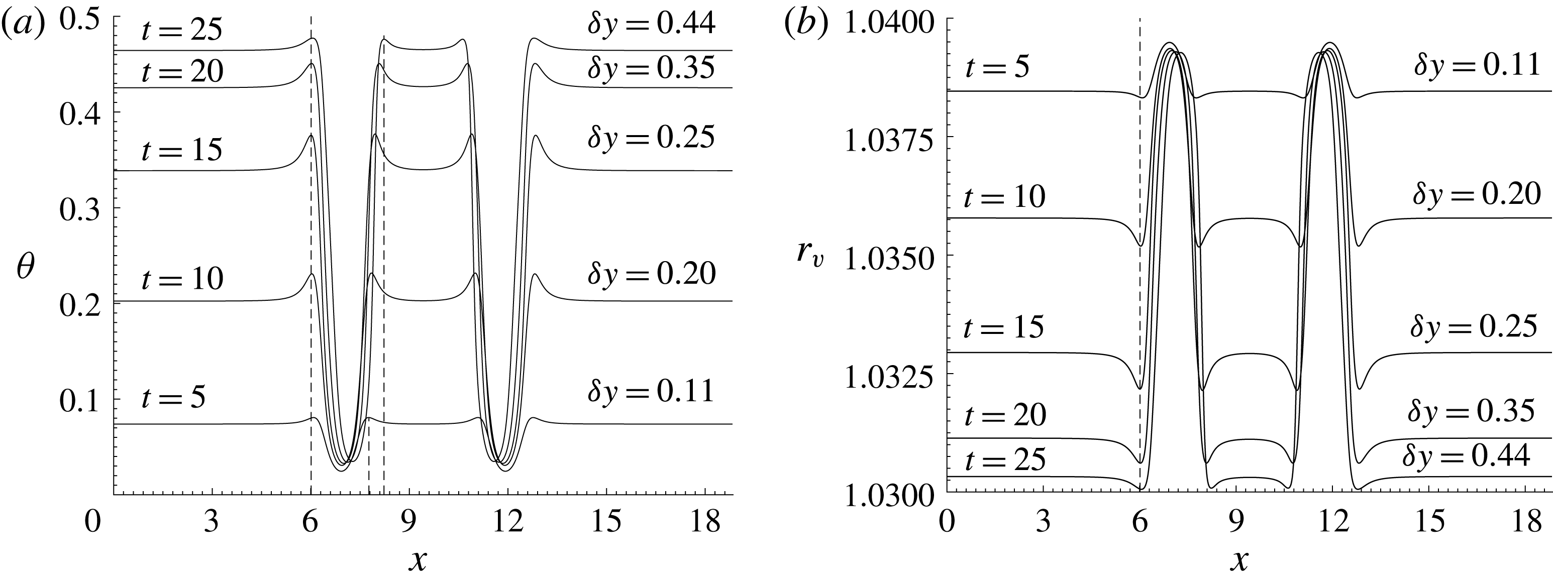
As soon as the simulation begins, the dynamics of the liquid leads the process. Figure 4 shows liquid mixing ratio profiles along horizontal lines passing through the locations of minimum liquid mixing ratio. It can be seen that by
 $t\approx 10$
, the vicinity of the vortices is almost entirely devoid of liquid. Also noticeable is the increase in liquid mixing ratio just outside the liquid-free voids thus created. Beyond this time there are very few condensation sites within these voids, and no significant further condensation occurring within them, even though there is supersaturated vapour present.
Everywhere else, the condensation process proceeds unhindered, raising the average temperature of the entire flow. The temperature and vapour mixing ratio profiles at different times are shown along a horizontal line moving with the vortex centroids in figure 5. Condensation being shut off near the vortices leads to this region remaining vapour rich in contrast to the rest of the flow, where vapour is continuously converted to liquid. Moreover, the vortices are now are colder than their surroundings, and therefore experience a negative buoyancy. This negative buoyancy causes, in combination with the vorticity, the lift force which propels the vortices laterally towards each other (see Ravichandran et al. (Reference Ravichandran, Dixit and Govindarajan2017) for more details). Like the liquid mixing ratio, the temperature and the vapour concentration show small blips of high temperature and low vapour concentration in the region just outside the vortices. The high liquid mixing ratio leads to higher rates of condensation within the rings than outside, and hence higher temperatures (and lower vapour mixing ratios) within the rings than elsewhere (see figure 5).
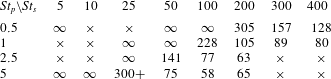
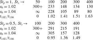
Table showing the times at which the kinetic energy reaches a minimum (which is a reasonable proxy for the annihilation time) for various combinations of
 $St_{s}$
and
 $St_{p}$
. Combinations for which simulations were carried out are marked with either a ‘
 $\infty$
’, suggesting that the lift-induced mechanism does not operate, or a finite value for the annihilation time. A ‘
 $\times$
’ indicates that no simulation was performed.
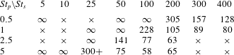
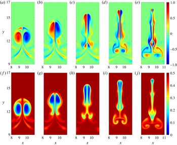
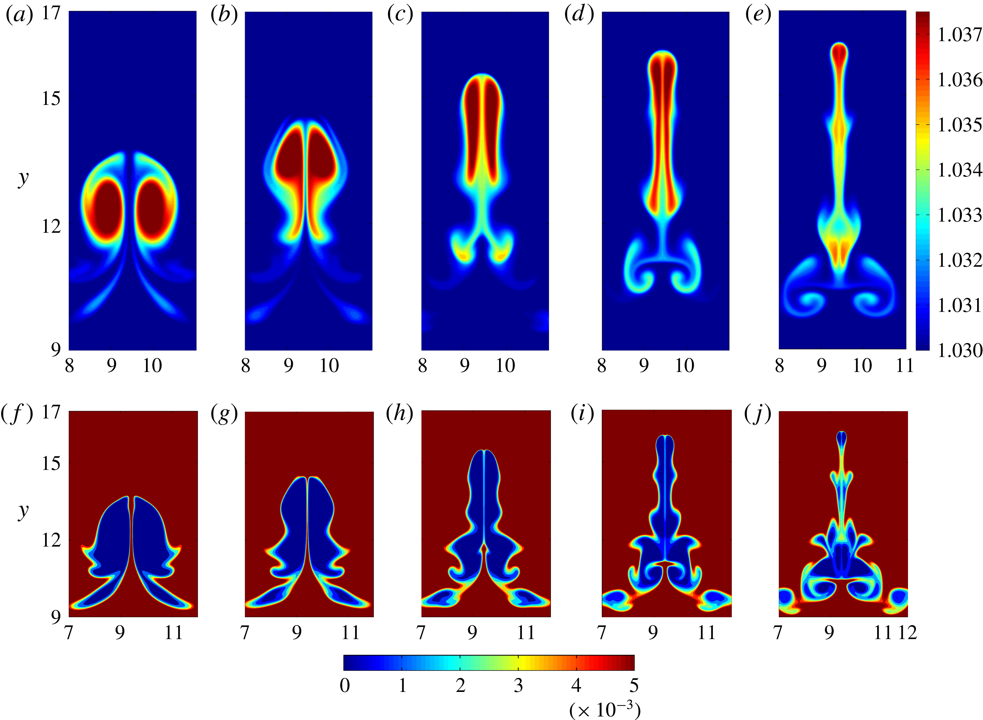
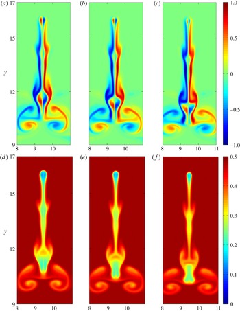
Contour plots of the vorticity and temperature at different later stages during their evolution are shown in figure 6, and those of vapour and liquid mixing ratio are shown in figure 7. The baroclinic torque produces vorticity of both signs on both sides of the symmetry plane. The same-signed vorticity that is produced merges into the original vortices, increasing their strength. Counter-signed vorticity produced near the original vortices acts to annihilate the vortices, while counter-signed vorticity produced in the tails remains behind. As the vortices come closer together, the original dipole withers away under the action of baroclinic torques, leaving the vapour (and temperature) patches to merge. Figure 8 shows the annihilation process at closely spaced time intervals around the time the dipole collapses, clearly showing both the annihilation of the vortices and the merger of the cold patches. Note that the time at which the original vortices are finally erased is different from the time at which the kinetic energy reaches a minimum (which is what is listed in table 2). The vortices are typically erased a little while after the kinetic energy reaches a minimum. As the cold and therefore dense vortices rise upwards, some kinetic energy of motion is converted to potential energy. This potential energy is then converted back into kinetic energy as the colder and denser fluid, carried with the now annihilated vortices, descends downwards.
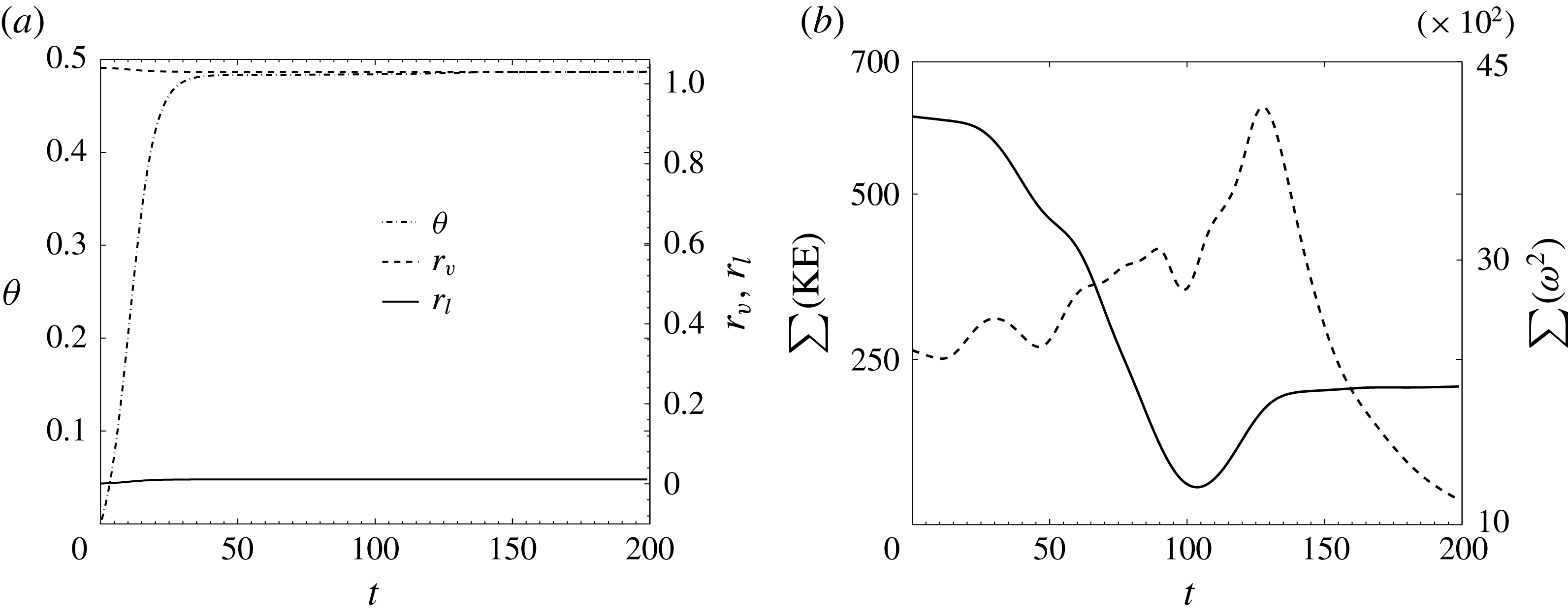
For comparison, box-averaged values of temperature, and vapour and liquid mixing ratios are shown in figure 9. Note that the system does not follow a canonical exponential relaxation to equilibrium – the equilibrium itself changes with time. As the temperature increases due to condensation, the saturation vapour mixing ratio increases too, meaning that the effective supersaturation of the system falls. This can be seen in the equilibrium value of the vapour mixing ratio, which is closer to
 $1.3$
than to
 $1$
. Consequently, the temperature reaches
 $95\,\%$
of its equilibrium value by
 $t=25$
, even though the nominal Stokes number is
 $St_{s}=200$
.
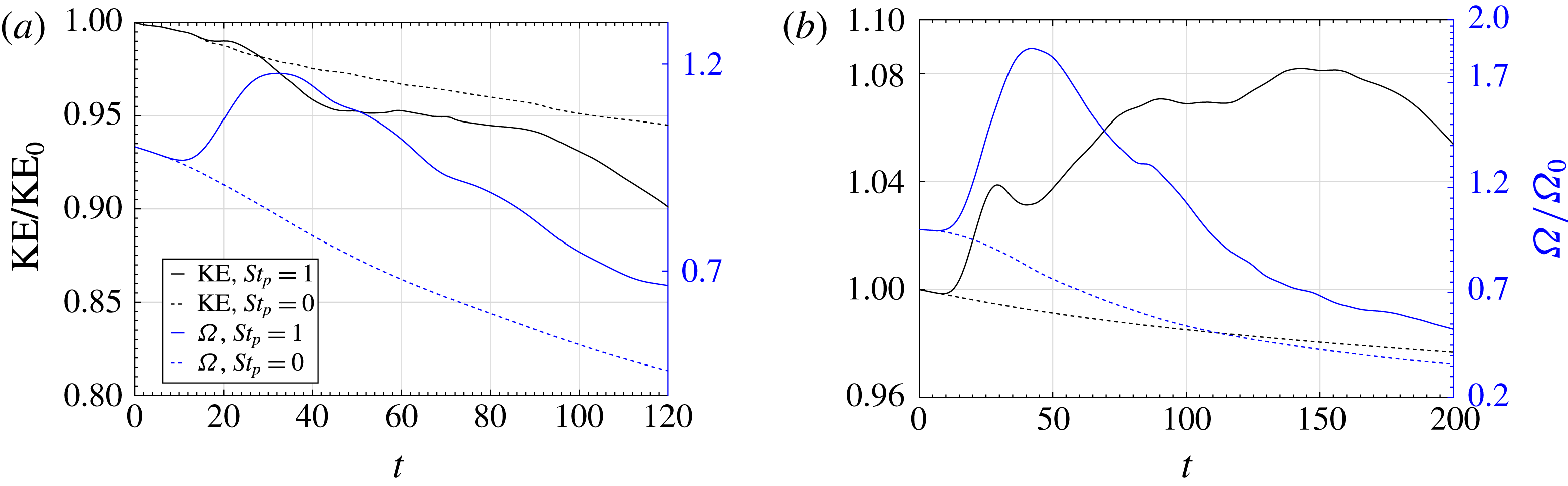
Also shown are in figure 9 are the average enstrophy and kinetic energy, showing a spike in enstrophy seen as a result of the creation of small-scale structures because of the collapse of the vortex dipole.
A sequence of snapshots showing the lift-induced vortex annihilation (description in text). The snapshots are shown at simulation times
 $t=80,90,100,110,120$
, respectively. Panels (a–e) show the vorticity
 $\unicode[STIX]{x1D714}$
, (f–j) show the temperature
 $\unicode[STIX]{x1D703}$
. The Stokes numbers were
 $St_{s}=200$
and
 $St_{p}=1$
. Note also that by approximately
 $t=110$
, the vorticity maximum has switched sides, relative to
 $t=0$
. See also figures 2 and 3.

Vapour mixing ratio
 $r_{v}$
(a–e), and liquid mixing ratio
 $r_{l}$
for the same time instants and initial conditions as in figure 6.

A sequence of snapshots showing details of the final stages of the annihilation of the vortices. Note that the actual erasure of the original vortices occurs after the kinetic energy has reached a minimum (at
 $t=105$
in this case; see table 2). Panels (a–c) show the vorticity
 $\unicode[STIX]{x1D714}$
, and (d–f) the temperature
 $\unicode[STIX]{x1D703}$
. at simulation times
 $t=121,123,125$
respectively.

 $St_{s}=200$
,
 $St_{p}=1$
. (a) The evolution of the (box-averaged) temperature (left axis) and the liquid and vapour mixing ratios (right axis) as a function of time. The temperature reaches
 $95\,\%$
of its equilibrium value by
 $t=25$
(also see figure 5). (b) The kinetic energy (left axis, solid line) and the enstrophy (right axis, dotted line) as a function of time. The dipole collapses at approximately
 $t=105$
, which is the time the kinetic energy reaches a minimum (see also table 2). Around the same time, the enstrophy begins to increase rapidly.

It is clear that if the liquid field is advected with no inertia, i.e. if we set
 $St_{p}=0$
, no regions devoid of liquid will form around the vortices. Without the voids, there will be no temperature difference between the vortices and the ambient, no buoyancy, and therefore no lift on the vortices, and consequently no collapse of the dipole. In fact,
 $St_{p}\neq 0$
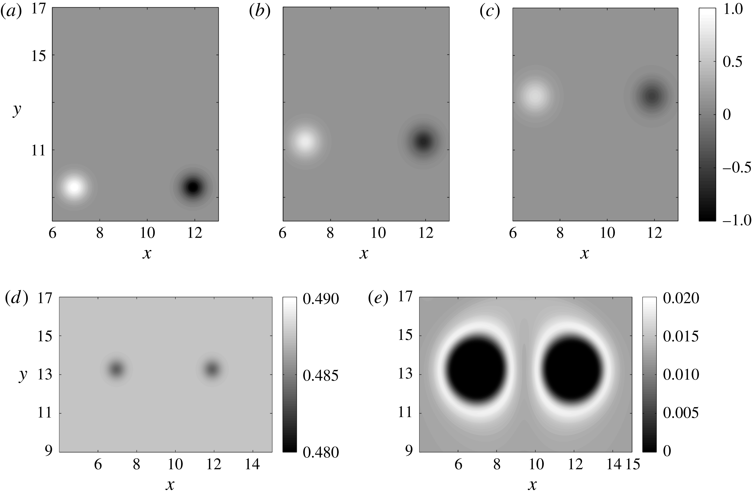
is not sufficient for the lift-induced mechanism to operate. We show this in figure 10, where
 $St_{p}=1$
,
 $St_{s}=25$
. It can be seen that although there are liquid-free voids because of the non-zero particle inertia, the fact that these voids do not form fast enough to make the vortices appreciably colder than the ambient means that no significant lift is generated by the vortices. This is a typical case when the combination of inertia and phase change do not induce a fundamental change in the dynamics.
Contour plots of
 $\unicode[STIX]{x1D714}$
at
 $t=0,100,200$
(a–c), showing the complete absence of any lateral drift for the vortices, for
 $St_{p}=1$
,
 $St_{s}=25$
. The reason for this is that the temperature difference between the vortices and the ambient is very small (d), even though the liquid-free void keeps growing in size (e).

3.1 Spanning the
 $St_{s}$
–
$St_{p}$
space


Table 2 shows the combinations of
 $St_{s}$
and
 $St_{p}$
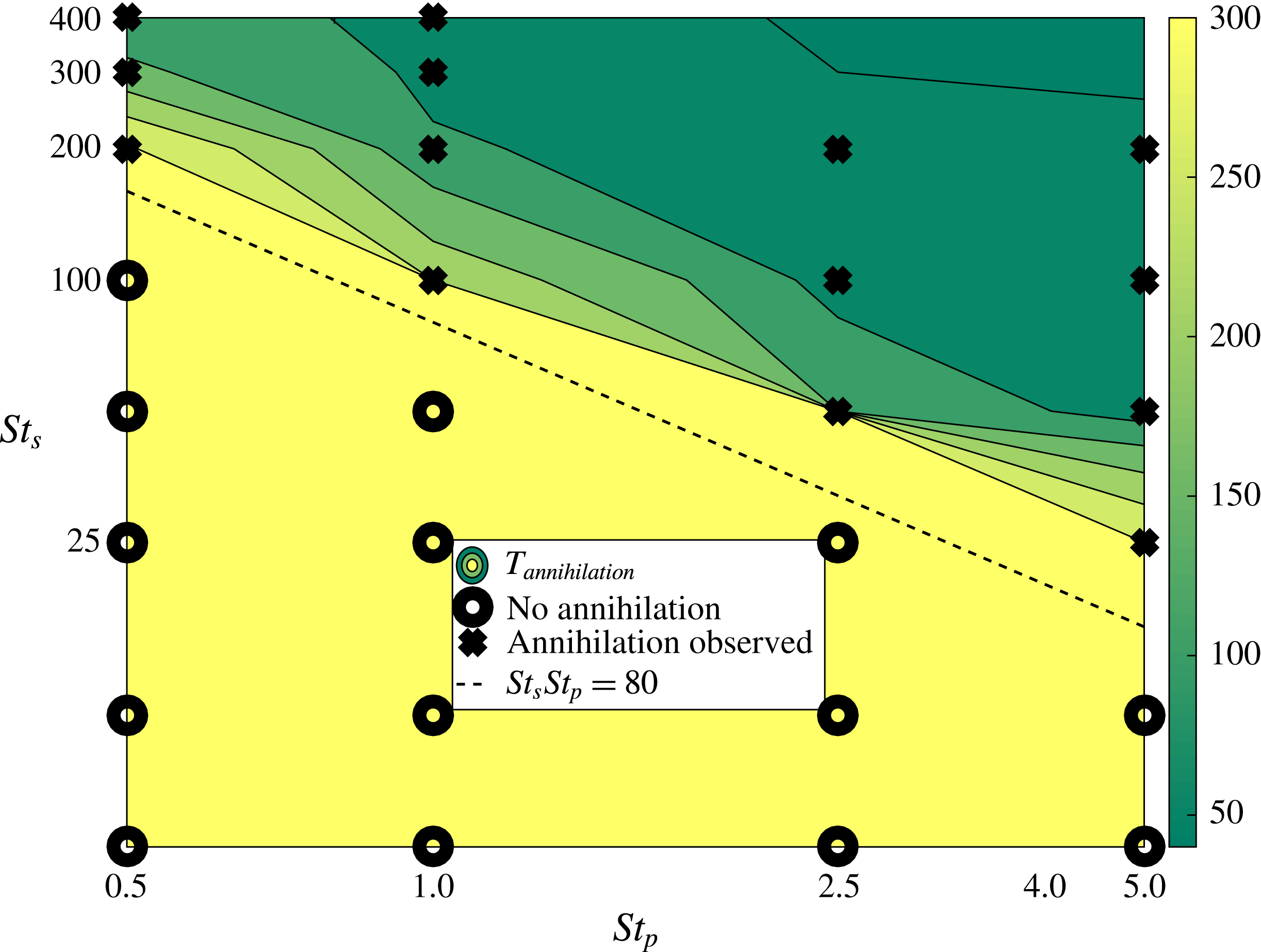
for which lift-induced vortex-dipole collapse occurs. The numbers given are the times at which the kinetic energy in the system reaches a minimum, since this is a reasonable proxy for the annihilation of the vortices of the dipole. An infinite value denotes that no annihilation occurred. Clearly, not all combinations of the Stokes numbers are viable for dipole collapse. This boundary is more readily seen in the plot in figure 11, which shows that there exists some value of
 $St_{s}$
, for every
 $St_{p}$
, below which the mechanism does not operate. In fact, the cutoff values for
 $St_{s}$
and
 $St_{p}$
are inversely related. We provide a theoretical reasoning for why this should be so in § 4. Beyond this cutoff value, the time of collapse is shown to decrease with increase in the product of the two Stokes numbers.
Plot showing a boundary in the
 $St_{s}{-}St_{p}$
plane where the lift-induced vortex-dipole collapse can occur as a result of particle inertia and thermodynamics. Crosses indicate that vortex annihilation was observed in the simulation. Noughts indicate that the buoyancy did not cause a fundamental change in the dynamics of the vortex dipole. The dashed line is a plot of the relation
 $St_{s}St_{p}=80$
.

3.2 Asymmetric initial conditions
Ravichandran et al. (Reference Ravichandran, Dixit and Govindarajan2017) discuss the effects of asymmetry in the initial conditions, and find that asymmetry effectively reduces the impact of the vortex annihilation. We discuss two ways in which the initial conditions can be asymmetric, and find that the observed behaviours are broadly consistent with the findings of Ravichandran et al. (Reference Ravichandran, Dixit and Govindarajan2017).
3.2.1 Orientation asymmetry
If the vortices in the dipoles are placed asymmetrically relative to the vertical (i.e. they are not at the same
 $y-$
coordinate), lift-induced collapse can still occur, provided that the asymmetry is not too large (Ravichandran et al.
Reference Ravichandran, Dixit and Govindarajan2017). We find that the behaviour with thermodynamics is similar. A representative case is shown in figure 12. The vertical separation between the vortices is
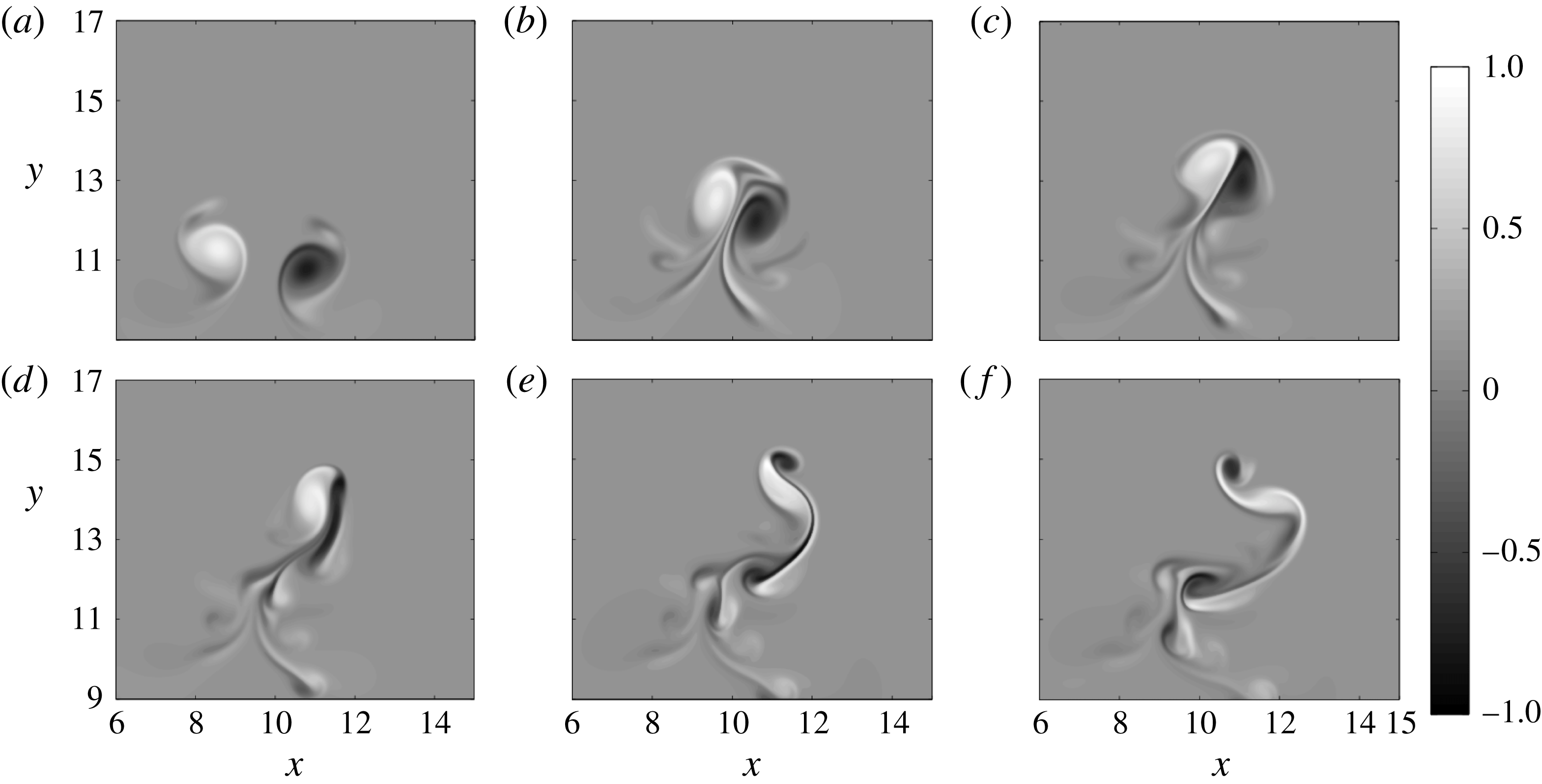
 $0.5d_{0}$
, making the vertical separation one-tenth of the horizontal separation. It can be seen that the sequence of events is markedly different from that in figure 6. In particular, unlike the annihilation of the vortices seen in figure 6, where the original vortices are erased due to the action of baroclinic torque, the vortices here are merely severely distorted. We found that for vertical separations
 ${\geqslant}d_{0}$
, the two vortices did not come close enough to annihilate.
A sequence of snapshots showing lift-induced vortex annihilation for asymmetric initial conditions. The snapshots are shown at simulation times
 $t=60,80,90,100,110,120$
(a–f, respectively). The Stokes numbers were
 $St_{s}=200$
and
 $St_{p}=1$
, and the vortices were initially separated by
 $5d_{0}$
and
 $0.5d_{0}$
horizontally and vertically, respectively.

3.2.2 Vortex size/strength asymmetry
If the vortices forming the dipole are different in strength or size (or both) relative to each other, the dynamics proceeds with predictable differences from the canonical case. The line joining the vortices first develops a tilt relative to the horizontal, owing to the stronger vortex creating a larger void around itself than the other. This vortex is colder, and has a larger negative buoyancy acting on it. From here, the dynamics proceeds similarly to the case in § 3.2.1 above.
3.3 Effect of magnitude of initial supersaturation
In all the simulations reported thus far, the initial supersaturation was
 $4\,\%$
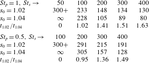
. Since the temperature difference between the vortices and its surroundings decides the density difference, and therefore the magnitude of the lift, we might expect that the time for merger would be proportionally larger with smaller supersaturation. However, the initial supersaturation decides, according to (2.8) and (2.12), both the magnitude of the final temperature change and the rate at which this final temperature is reached. Halving the initial supersaturation would therefore halve the final temperature
 $\unicode[STIX]{x1D703}_{t\rightarrow \infty }$
that is reached, and also roughly double the time taken to reach this temperature. Doubling the time taken amounts to doubling
 $St_{s}$
, the phase-change Stokes number. These two effects of smaller supersaturation seem to act against each other (see also § 4 and figure) as far as the collapse of the vortex dipole is concerned, and the time for annihilation
 $t_{1.02}$
for simulations starting with
 $s_{0}=1.02$
is of the same order of magnitude as that (
 $t_{1.04}$
) for simulations starting with
 $s_{0}=1.04$
. This can be seen in table 3. In fact, in one case (
 $St_{s}=50$
,
 $St_{p}=1$
), the smaller initial supersaturation produces lift-induced collapse even when the higher initial supersaturation does not.
Effect of the initial supersaturation on the times to dipole collapse. The notation is the same as in table 2, and
 $t_{1.02}$
and
 $t_{1.04}$
are the times for dipole collapse for simulations starting with initial supersaturations of
 $2\,\%$
and
 $4\,\%$
, respectively.
3.4 Many-vortex simulations
We have demonstrated a mechanism by which particle inertia and phase change combine to create a fundamental change in the dynamics of a pair of counter-signed vortices, including a collapse of large-scale vortices and the creation of baroclinic torque at small scales during the collapse. We now wish to study the effect of coupling of particle inertia and phase change on two-dimensional turbulence. As a proxy for 2D turbulence, we use the dynamics of many vortices. We report simulations of many with
 $St_{s}=200$
and
 $St_{p}=0$
or 1, comparing the results with and without particle inertia. The simulations reported were performed in periodic boxes of size
 $L=20$
, with
 $Fr^{2}=25$
, at two Reynolds numbers,
 $Re=5000$
and
 $Re=20\,000$
. The
 $Re=5000$
simulations were done with
 $2048\times 2048$
collocation points, and the
 $Re=20\,000$
simulations with
 $4096\times 4096$
collocation points. The simulations were started with
 $50$
vortices each of positive and negative signed vorticity. We have used two types of initial conditions for the many-vortex simulations, one in which the vortex strengths are chosen from a distribution with a given mean (such that the mean strength gives the Reynolds number required), and the other in which the strengths are all the same. We find similar results with either initial condition. Identical initial conditions are used for simulations with or without particle inertia.
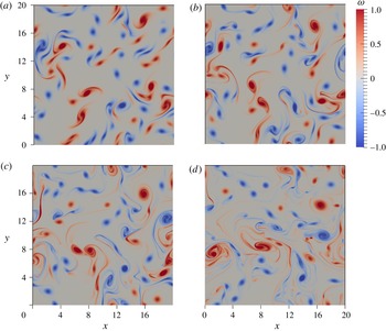
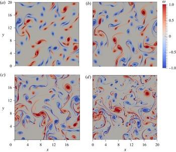
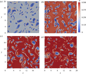
The analogues of figures 6 and 7 are shown in figures 13–15 for
 $Re=5000$
, and figures 16–18 for
 $Re=20\,000$
. For the case without particle inertia, the temperature, vapour mixing ratio and liquid mixing ratio are uniform in the domain, leaving only the vorticity; this is shown in figure 13. For the case with particle inertia
 $(St_{p}=1)$
, the familiar dynamics of centrifugal expulsion of the liquid, followed by patches of lower temperature and higher vapour concentration is seen. Thus the mechanism leading to density and buoyancy differences is that same as before. In fact, given that the parameters in our many-vortex simulations are defined based on the characteristics of one typical vortex in the system, the same relationship of
 $St_{p}$
and
 $St_{s}$
as earlier (§§ 3.1 and 4.1) decides whether buoyancy forces will contribute to the flow. We note however that while annihilation events are clearly visible (we count approximately half a dozen in each simulation), vortex-dipole annihilation is not the primary consequence of buoyancy inhomogeneities. This could be expected from the results of § 3.2.1. The presence of buoyancy drives smaller scales in other ways as well.
Vorticity and temperature plots for (
 $Re=5000$
,
 $St_{p}=1$
,
 $St_{s}=200$
) are shown in figures 14 and 15, respectively. The vapour and liquid mixing ratio plots can be found in the supplementary material available at https://doi.org/10.1017/jfm.2017.677, along with a movie showing the evolution of all four quantities. We see that until approximately
 $t=20$
, the vorticity plots look similar in figures 13 and 14. After the temperature difference between the vortices and the ambient is established, the dynamics become different, leading to significant distortion of the vortices and smaller scales in the case with particle inertia. Some merger events for
 $Re=5000$
are pointed to in figure 14. Figures 16 and 17 show the vorticities for the simulations with
 $St_{p}=0$
and
 $St_{p}=1$
, respectively, and figure 18 shows the temperature plots, for
 $Re=20\,000$
. The vapour and liquid plots are available in the supplementary material.
The differences in the dynamics between the cases with and without inertia for
 $Re=5000$
(figures 13 and 14) are not prominent, although smaller scales are enhanced, as will be clearly seen in the spectra. These differences for
 $Re=20\,000$
, however, are drastic, with the
 $St_{p}=1$
simulations showing significantly greater production of small-scale structures.
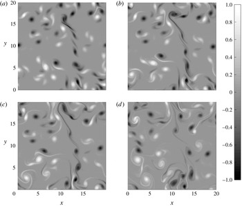
A sequence of snapshots showing the evolution of the vorticity of a system of many vortices at
 $Re=5000$
. The snapshots are shown at simulation times
 $t=10,20,30,50$
(a–d, respectively). The Stokes numbers were
 $St_{s}=200$
and
 $St_{p}=0$
. The corresponding vorticity plots for the case with inertia
 $(St_{p}=1)$
are shown in figure 14.

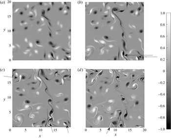
A sequence of snapshots showing the evolution of the vorticity of a system of many vortices at
 $Re=5000$
. The snapshots are shown at simulation times
 $t=10,20,30,50$
(a–d, respectively). The Stokes numbers were
 $St_{s}=200$
and
 $St_{p}=1$
. The corresponding vorticity plots for the case without particle inertia
 $(St_{p}=0)$
are shown in figure 13. Note that until approximately
 $t=20$
, the systems with and without inertia look similar, since it takes the thermodynamics time to take effect. The arrows point to annihilation events.

A sequence of snapshots showing the evolution of the temperature in the same system as in figure 14. The snapshots are shown at simulation times
 $t=10,20,30,50$
(a–d, respectively). The Stokes numbers were
 $St_{s}=200$
and
 $St_{p}=1$
.

A sequence of snapshots showing the evolution of the vorticity of a system of many vortices, with parameters
 $Re=20\,000$
,
 $St_{s}=200$
and
 $St_{p}=0$
. The snapshots are shown at simulation times
 $t=10,20,30,50$
(a–d, respectively). The corresponding vorticity plots for the case with particle inertia
 $(St_{p}=1)$
are shown in figure 17.

A sequence of snapshots showing the evolution of a system of many vortices, with parameters
 $Re=20\,000$
,
 $St_{s}=200$
and
 $St_{p}=1$
. The snapshots are shown at simulation times
 $t=10,20,30,50$
(a–d, respectively). The corresponding vorticity plots for the case without particle inertia are shown in figure 16.

A sequence of snapshots showing the evolution of the temperature in the same simulation shown in figure 17 (
 $Re=20\,000$
,
 $St_{s}=200$
and
 $St_{p}=1$
). The snapshots are shown at simulation times
 $t=10,20,30,50$
, respectively.

Figure 19 shows the evolution of the average kinetic energy and enstrophy in simulations with and without inertia for
 $Re=5000$
and
 $Re=20\,000$
. For both Reynolds numbers, for
 $t\lesssim 20$
– i.e. before significant condensation has occurred – the evolution of the two simulations is similar. After
 $t\approx 20$
, the simulations with particle inertia, owing to the density differences created, see a significant growth in enstrophy. In the
 $Re=5000$
simulation, the kinetic energy, is lower for the system with particle inertia, whereas the kinetic energy is higher with inertia for
 $Re=20\,000$
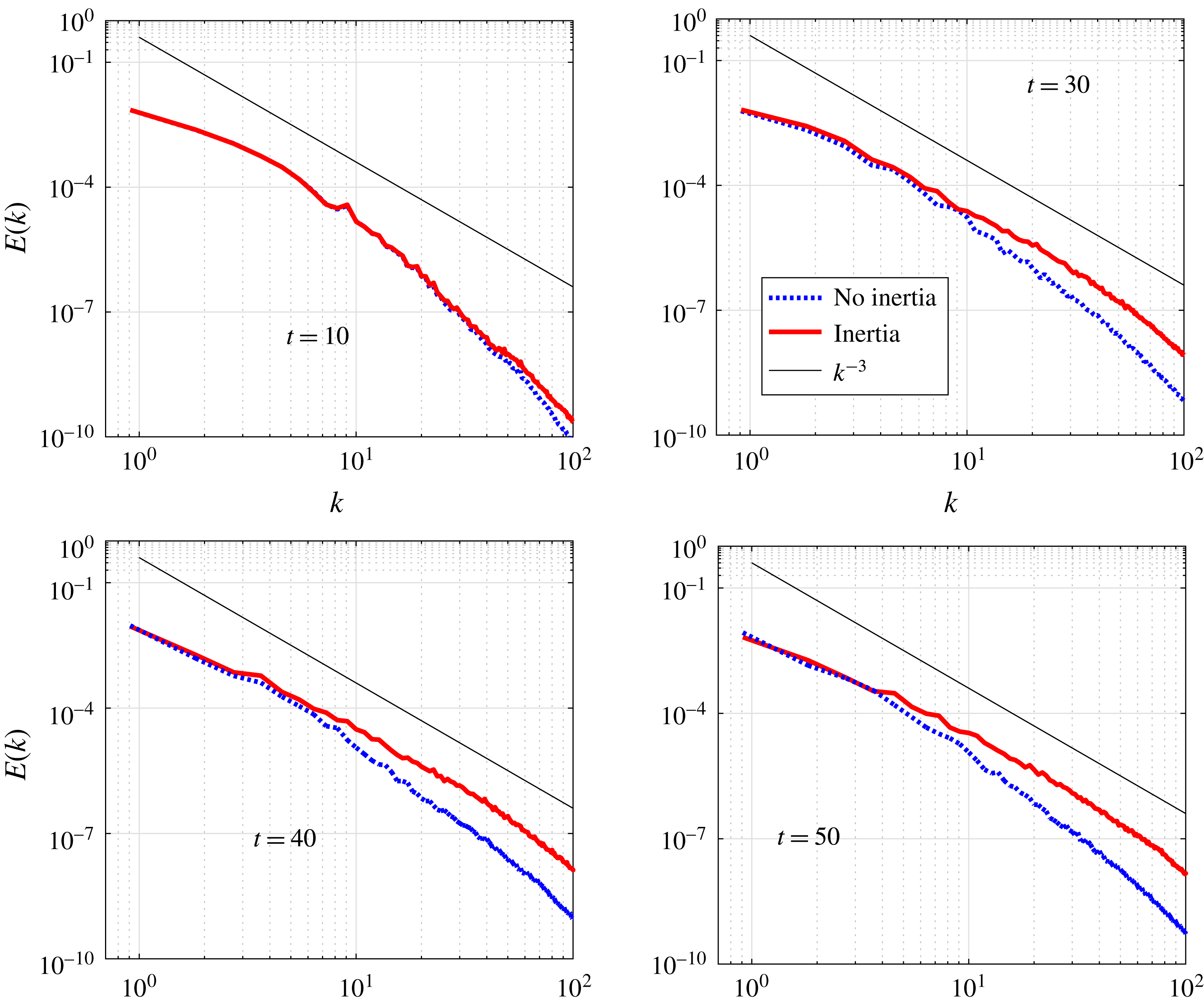
. Figure 20 shows the spectra of the kinetic energy for simulations with and without inertia at
 $Re=20\,000$
. A similar plot for
 $Re=5000$
can be found in the supplementary material. It is clear that the addition of particle inertia moves energy into smaller scales in the flow, and that the scaling is closer to
 $k^{-3}$
with inertia. These spectra may be compared to figure 10 in Ravichandran et al. (Reference Ravichandran, Dixit and Govindarajan2017) to find, again, that the differences not quite as stark.
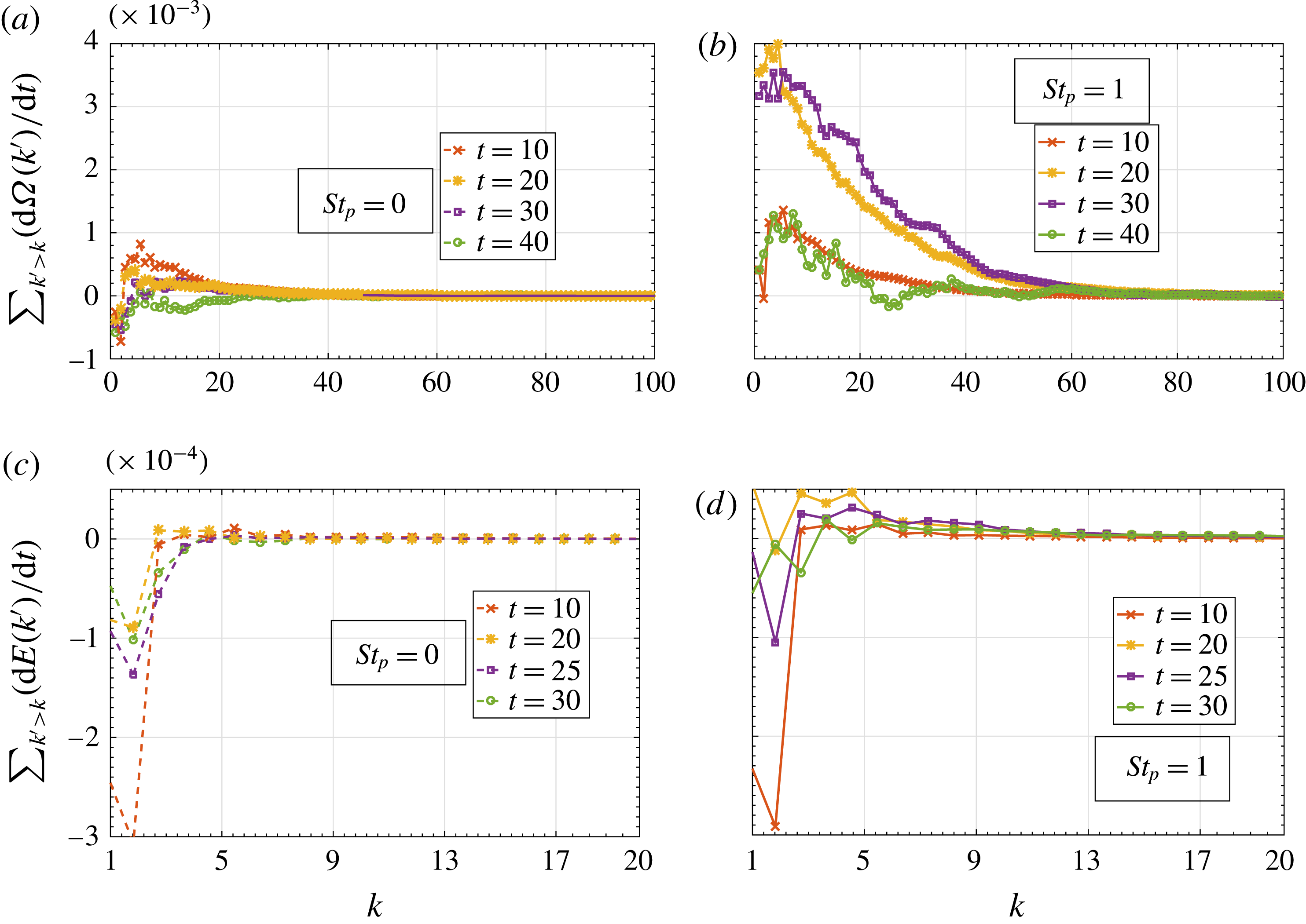
We also plot the rates of change of energy and enstrophy spectral density (
 $E(k)$
and
 $\unicode[STIX]{x1D6FA}(k)$
respectively) as a function of the wavenumber for the simulations at
 $Re=20\,000$
in figure 21. These rates were calculated by adding the rates of change of energy and enstrophy at all modes with a wavenumber higher than a given wavenumber. Therefore, a positive value at a given wavenumber
 $k$
means that energy or enstrophy is increasing for wavenumbers higher than
 $k$
. Note that the quantities plotted are not zero at
 $k=0$
, since viscous and buoyancy-driven contributions are included. The times at which the fluxes are plotted are chosen such that the kinetic energy or enstrophy are climbing steeply (see figure 19). It can be seen clearly that the addition of particle inertia increases the transfer of enstrophy to smaller scales significantly.
The average kinetic energy (left axis) and enstrophy (right axis) in simulations starting with identical initial conditions in identical boxes. Both simulations have phase-change Stokes number
 $St_{s}=200$
. The particle Stokes numbers were
 $St_{p}=0$
(dashed lines) and
 $St_{p}=1$
(solid lines). (a)
 $Re=5000$
, (b)
 $Re=20\,000$
. For both Reynolds numbers, the enstrophy increases significantly for the case with non-zero particle inertia.

The kinetic energy spectra for simulations with and without particle inertia for
 $Re=20\,000$
. Dashed lines show simulations with
 $St_{p}=0$
, and are seen to have lesser energy at higher wavenumbers.
 $k^{-3}$
lines are shown for references.

The kinetic energy and enstrophy fluxes for the simulations with
 $Re=20\,000$
. The enstrophy flux plots (a,b) show that enstrophy is transferred to higher wavenumbers preferentially for the case with
 $St_{p}=1$
. The kinetic energy flux plots (c,d) also show the same behaviour, but for a smaller band of wavenumbers.

4 Discussion
4.1 Effective Atwood number
We now analyse whether we can predict the region of parameter space where the action of Kutta lift on the dipole becomes significant. As we have seen in § 2.4, buoyant vortices experience lift forces as a result of the velocity relative to the fluid they pick up under the influence of buoyancy. Their dynamics is governed by the combined action of the forces of lift and buoyancy, and is parametrised by the Atwood number. If the buoyancy that drives this dynamics arises out of the thermodynamics of phase change, the effective Atwood number is a function both of the maximum temperature difference between the inside of the patch and the ambient and the size of this patch.
 $$\begin{eqnarray}A_{eff}=\frac{\unicode[STIX]{x1D703}_{eq}}{T_{0}}\left(\frac{r_{patch}}{r_{vor}}\right)^{2}.\end{eqnarray}$$
The maximum temperature difference
 $\unicode[STIX]{x1D703}_{eq}$
is a fixed quantity given the initial supersaturation. The size of the patch is given by the area around the vortex cleared out because of particle inertia. The radius, it can be shown (see, e.g. Ravichandran & Govindarajan Reference Ravichandran and Govindarajan2015), will be proportional to
 $$\begin{eqnarray}r_{patch}\sim \left(\frac{\unicode[STIX]{x1D6E4}^{2}\unicode[STIX]{x1D70F}_{p}t}{4\unicode[STIX]{x03C0}^{2}}\right)^{1/4}=\left(\frac{(\unicode[STIX]{x03C0}r_{vor}^{2}\unicode[STIX]{x1D6FA}_{0})^{2}\unicode[STIX]{x1D70F}_{p}t}{4\unicode[STIX]{x03C0}^{2}}\right)^{1/4}.\end{eqnarray}$$
The particle have a time
 $t$
above that is proportional to the phase relaxation time scale
 $\unicode[STIX]{x1D70F}_{s}$
to vacate the vicinity of the vortex; the ratio of the area of the density patch to the area of the vortex then is
 $$\begin{eqnarray}\left(\frac{r_{patch}}{r_{vor}}\right)^{2}=\left(\frac{\unicode[STIX]{x1D6FA}_{0}^{2}\unicode[STIX]{x1D70F}_{p}\unicode[STIX]{x1D70F}_{s}}{4}\right)^{1/2}=\left(\frac{(\unicode[STIX]{x1D714}_{0}\unicode[STIX]{x1D70F}_{p})^{2}(\unicode[STIX]{x1D70F}_{s}/\unicode[STIX]{x1D70F}_{p})}{4}\right)^{1/2}\sim St_{p}^{1/2}St_{s}^{1/2}.\end{eqnarray}$$
The effective Atwood number is thus proportional to the square roots of both the droplet-inertia and phase-change Stokes numbers. We find that this simple analysis is reasonably good at predicting whether lift-induced vortex dipoles will merge. This was shown in figure 11, in which we plot the boundary for lift-induced merger in
 $St_{s}{-}St_{p}$
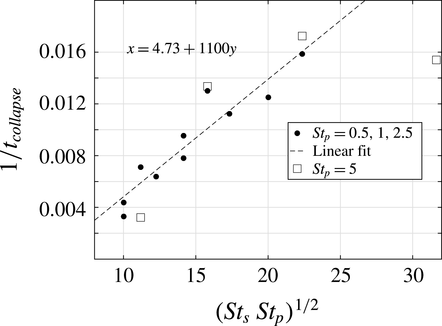
space. It can also be seen from a plot of the (inverses of the) annihilation times in table 2 plotted against
 $(St_{p}St_{s})^{1/2}$
. This is shown in figure 22. A linear fit is shown as well, whose intercept on the
 $x$
-axis gives the minimum value for which the lift-induced vortex-dipole collapse mechanism can be activated by particle inertia. The points marked by squares instead of circles are points for which
 $St_{p}=5$
, and using (2.16) for the motion of the liquid field would be suspect.
Alternatively, consider the time it takes for a void of a characteristic size
 $r_{vor}$
to form. This is given by the same relation between radius and time as above:
 $$\begin{eqnarray}t_{void}=\frac{4\unicode[STIX]{x03C0}^{2}r_{vor}^{2}}{\unicode[STIX]{x1D6E4}^{2}\unicode[STIX]{x1D70F}_{p}}\;\Longrightarrow \;\unicode[STIX]{x1D6FA}_{0}t_{void}=\frac{4}{\unicode[STIX]{x1D6FA}_{0}\unicode[STIX]{x1D70F}_{p}}.\end{eqnarray}$$
In this time, the temperature everywhere in the flow would have gone up by an amount proportional to
 $$\begin{eqnarray}\unicode[STIX]{x1D703}_{in}=\frac{0.04}{\unicode[STIX]{x1D70F}_{s}}t_{void}\sim \frac{1}{\unicode[STIX]{x1D6FA}_{0}^{2}\unicode[STIX]{x1D70F}_{p}\unicode[STIX]{x1D70F}_{s}}=\frac{1}{St_{p}St_{s}},\end{eqnarray}$$
where
 $0.04$
is the initial supersaturation. After
 $t_{void},$
the temperature in the void remains the same, whereas the temperature everywhere else in the box reaches the equilibrium value. The effective Atwood number is then given by the difference between
 $\unicode[STIX]{x1D703}_{in}$
and the equilibrium temperature
 $\unicode[STIX]{x1D703}_{eq}$
. Therefore, the larger the value of
 $St_{p}St_{s}$
, the smaller the value of
 $\unicode[STIX]{x1D703}_{in}$
, and the greater the difference between
 $\unicode[STIX]{x1D703}_{in}$
and
 $\unicode[STIX]{x1D703}_{eq}$
.
Plot of vortex annihilation times as a function of the parameter
 $(St_{s}St_{p})^{1/2}$
. A linear fit is shown, providing a minimum value for
 $(St_{s}St_{p})^{1/2}$
below which our mechanism will not operate.

4.2 Effect of supersaturation
As we saw in § 3.3, the effect of using a different supersaturation is non-trivial. The two effects of halving the supersaturation are to halve the maximum temperature reached and to double the time taken to reach the maximum temperature. These effects, for the reasons sketched in § 3.3, compete against each other. We can estimate that halving the supersaturation should lead to the effective Atwood number falling by a factor of
 $\sqrt{2}$
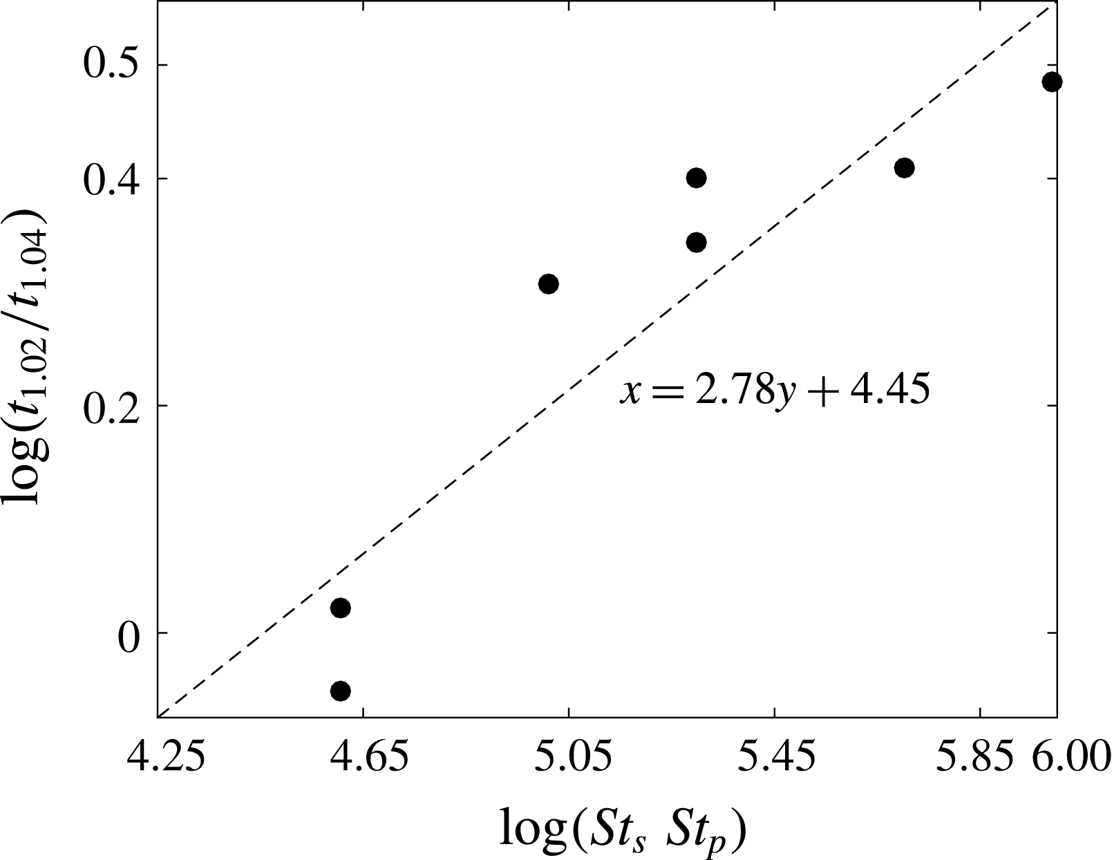
. A plot of the values in table 3 shows (figure 23) that this factor is in fact not constant, and falls to
 $1$
at the edge of the region where the lift-induced mechanism applies. The power-law dependence
 $t_{1.02}/t_{1.04}\sim (St_{s}St_{p})^{1/3}$
is as yet unexplained.
The ratio of vortex-dipole collapse times for two different values of the initial supersaturation plotted against the product of the Stokes numbers, showing an as yet unexplained power-law dependence. Note that the
 $x$
-intercept here is roughly the same as the boundary at which the mechanism stops working (see figure 11). We have not found an explanation for the exponent
 ${\approx}1/3$
.

4.3 Effect of Reynolds number
As we discuss in § 2, the time for vortex-dipole collapse is independent of the Reynolds number, being dependent only on the inverse of the Froude number. However, in the case of many vortices, the results of § 3.4 show that the Reynolds number has a significant effect on the dynamics of the buoyant vortices.
4.4 Relevance to clouds
We now also discuss applications to cloud-like situations. A typical cumulus cloud has droplets of approximately
 $10{-}20~\unicode[STIX]{x03BC}$
m radius (see, e.g. Pruppacher, Klett & Wang Reference Pruppacher, Klett and Wang1998). This makes the inertia of the droplets
 $\unicode[STIX]{x1D70F}_{p}=O(10^{-2}{-}10^{-3})~\text{s}$
. The phase relaxation time scale is estimated as follows. Assuming typical values for
 $r_{s}^{0}=0.02,$
and
 $n=O(10^{8})~\text{m}^{-3}$
gives, for the phase relaxation time scale,
 $\unicode[STIX]{x1D70F}_{s}=O(10)~\text{s}$
. For
 $20~\unicode[STIX]{x03BC}$
m droplets, assuming
 $n=O(10^{6})~\text{m}^{-3}$
gives
 $\unicode[STIX]{x1D70F}_{s}=O(100)~\text{s}$
. The Stokes numbers
 $St_{s}$
and
 $St_{p}$
are also functions of the strength of the vortex being considered. Specifically, for water droplets to have particles Stokes numbers
 $O(1)$
, vortices typical of the Kolmogorov spectrum will require the particles to be
 $50{-}100~\unicode[STIX]{x03BC}$
m in size. At these sizes, gravitational settling (which we have ignored) would dominate the dynamics of the droplets (see, e.g. Rosa et al.
Reference Rosa, Parishani, Ayala and Wang2016). It is clear, therefore, that our mechanism is only valid for large values of vorticity, in particular of the kind found in vortex filaments.
Vortex filaments are ubiquitous in turbulence and are caused by vortex stretching and intermittency (Jiménez et al. Reference Jiménez, Wray, Saffman and Rogallo1993; Ishihara et al. Reference Ishihara, Kaneda, Yokokawa, Itakura and Uno2007). These long-lived filaments are known to have significantly higher values of vorticity than predicted by the Kolmogorov spectrum (Ishihara et al. Reference Ishihara, Kaneda, Yokokawa, Itakura and Uno2007; Yeung, Donzis & Sreenivasan Reference Yeung, Donzis and Sreenivasan2012). Their lifetimes, as reported by Douady, Couder & Brachet (Reference Douady, Couder and Brachet1991), are of the order of several large-eddy turnover times. A simple proof-of-concept calculation follows.
The Stokes numbers associated with droplets would be
 $O(1)$
for
 $\unicode[STIX]{x1D6FA}_{0}=O(1/\unicode[STIX]{x1D70F}_{p})=O(100~\text{s}^{-1})$
. If this vorticity is associated with a vortex filament whose strength is ten times the value dictated by the Kolmogorov spectrum, we can infer the length and time scales where this will happen. Consider a length
 $l$
and its corresponding time scale
 $t_{l}$
by Kolmogorov scaling arguments. For a dissipation rate of
 $\unicode[STIX]{x1D716}=10^{-1}~\text{m}^{2}~\text{s}^{-3}$
, it may be shown that
 $t_{l}=0.1~\text{s}$
and
 $l=1~\text{cm}$
are the length and time scales which will work for the model we have considered. Similarly,
 $l\approx 3~\text{mm}$
for
 $\unicode[STIX]{x1D716}=10^{-2}~\text{m}^{2}~\text{s}^{-3}$
. These values for the dissipation rates are representative values from table 1. These length scales fall in the inertial range of turbulence for typical conditions.
It can also be seen that for the vorticity and length scales cited above, the approximation of neglecting the gravity term for the droplets is valid, since the relevant ratio between gravitational-to-centrifugal acceleration is
 $1/100$
and
 $1/3$
.
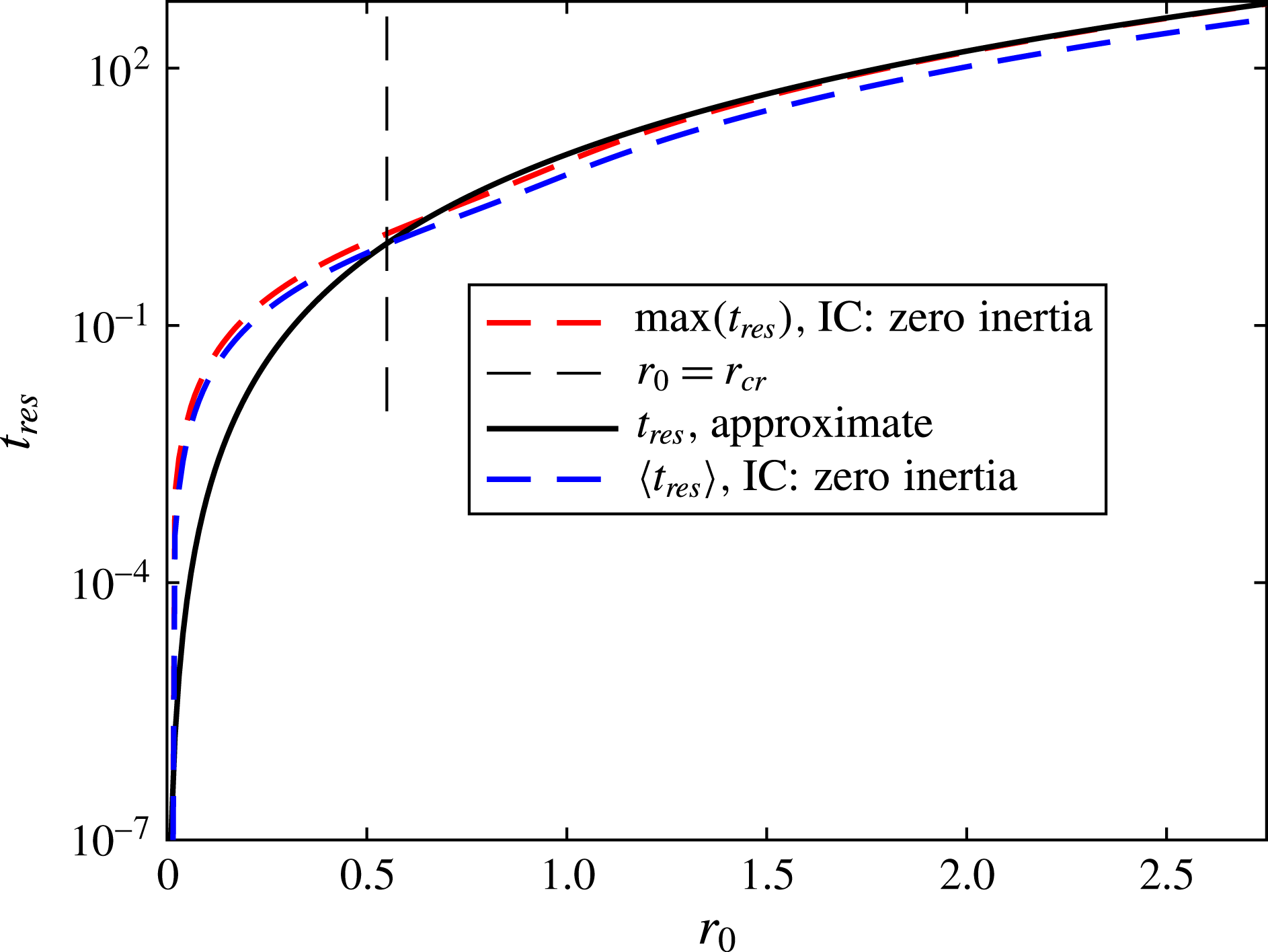
Time required for a void of a given radius to form, showing that the use of the approximate equation for particle dynamics does not lead to great errors. The two measures for the void-formation time (in the case where the particle dynamics is not approximated) are the maximum time required for every particle starting within a given radius to leave that radius (
 $\max (t_{res})$
) and the average time required for an initially uniform-in-space distribution of particles to leave a region within a given radius from a vortex (
 $\langle t_{res}\rangle$
). The two measures do not differ greatly either from each other or from the void-formation time implied by (2.16) (see § 4.1).

As an extreme case, consider
 $l=10~\text{cm},t_{l}=1~\text{s}$
for
 $\unicode[STIX]{x1D716}=10^{-2}~\text{m}^{2}~\text{s}^{-3}$
. If we have
 $20~\unicode[STIX]{x03BC}$
m droplets, we have
 $\unicode[STIX]{x1D6FA}_{0}=10/t_{l}=O(10~\text{s}^{-1}),St_{p}=O(0.1),St_{s}=O(1000).$
In this case, the gravity-to-centrifugal ratio is
 $1$
, and we may not be justified in dropping the gravitational settling term.
5 Conclusion
We show the occurrence of lift-induced vortex-dipole collapse in the presence of thermodynamics and particle inertia. We show that the centrifuging out of droplets from vortical regions leads to the creation of higher-density regions due to preferential phase change outside these regions, which enables lift to act on the vortices. We derive a scaling relationship which shows that this can happen when the product of the droplet-inertia Stokes number and the phase-change Stokes number crosses a threshold value, and show that our simulations agree with this analysis. The mechanism described here connects the microphysical quantity of droplet inertia to the dynamics of vortices which represent the large-scale dynamics in turbulent flow. For this reason, apart from the simplicity of the physical description behind the mechanism, we think this problem is worth further study, especially in terms of an extension to three dimensions. Preliminary results from three-dimensional simulations without thermodynamics suggest that the lift on buoyant vortices can alter the dynamics of vortex reconnection.
Acknowledgements
This work is partially supported by the Ministry of Earth Sciences, Government of India, under the Monsoon Mission Project on the Bay of Bengal. Computational resources from CSIR-4PI are gratefully acknowledged. Comments from the anonymous referees helped improve the paper and we thank them.
Supplementary material and movie
Supplementary material and a movie are available at https://doi.org/10.1017/ jfm.2017.677
Appendix A. Errors from using the inertial approximation, equation (2.16)
We now comment on the use of the simplified equation for droplet dynamics. Heavy inertial particles, under the influence of the Stokes drag, obey the equation of motion
 $$\begin{eqnarray}\frac{\text{d}\boldsymbol{v}}{\text{d}t}=\frac{\boldsymbol{u}-\boldsymbol{v}}{\unicode[STIX]{x1D70F}}.\end{eqnarray}$$
In this work, we have used (2.16) instead. It may be shown that the inertial approximation is valid when applied to a region outside the critical caustics radius (see Ravichandran & Govindarajan Reference Ravichandran and Govindarajan2015 for details). This radius is given by
 $r_{cr}\approx 0.5\sqrt{\unicode[STIX]{x1D71E}\unicode[STIX]{x1D70F}}$
. For the cases considered in this paper,
 $\unicode[STIX]{x1D71E}=\unicode[STIX]{x03C0}/4\approx 0.78$
, and
 $\unicode[STIX]{x1D70F}=O(1)$
. This means that the inertial approximation should not, by rights, be applied within a radius of approximately
 $0.45$
of the centres of the vortices. The vortices themselves have radii of
 $0.5$
. This means that the inertial approximation should not, strictly, be used as long as the voids where the liquid mixing ratio is zero are smaller than the vortices.
However, what matters for present purposes is the time it takes for the voids around the vortices to form. It can be seen from figure 24 that the use of the inertial approximation instead of the full equation does not significantly affect the time it takes for a void of a given radius to form.