2 Mathematical model

Given a DSSC of thickness d, the electron density 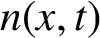$n(x, t)$ at position 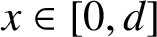$x \in [0, d]$ and time $t \geq 0$ satisfies the FPDE [Reference Maldon, Lamichhane and Thamwattana27]

(2.1) $$ \begin{align} \frac{\partial n}{\partial t} = D_{0}\frac{\partial^{1 - \gamma} }{\partial t^{1 - \gamma}}\frac{\partial^{2} n}{\partial x^{2}} +\varphi \alpha e^{-\alpha x} - k_R(n(x, t) - n_{\text{eq}}), \end{align} $$

where $D_{0}$ is the diffusion coefficient, $\gamma $ is the exponent in the mean-square displacement of the CTRW simulation of the semiconductor, $\varphi $ is the incident photon flux, $\alpha $ is the dye absorption coefficient, $k_R$ is the recombination constant and $n_{\text {eq}}$ is the dark equilibrium electron density. Equation (2.1) is subject to the boundary conditions

(2.2) $$ \begin{align} n(0, t) &= n_0 = n_{\text{eq}}e^{{qV_B}/{m_I k_B T}}, \end{align} $$

(2.3) $$ \begin{align} \frac{\partial n}{\partial x}\bigg|_{x = d}& = 0, \end{align} $$

(2.4) $$ \begin{align} n(x, 0)& = n_0, \end{align} $$

where q is the electron charge, $V_B$ is the bias voltage, $m_I$ is the diode ideality factor, $k_B$ is Boltzmann’s constant [Reference Anta, Idígoras, Guillén, Villanueva-Cab, Mandujano-Ramirez, Oskam, Pellejá and Palomares3] and T is the temperature of the DSSC.

We note that under the special case $\gamma = 1$ , we recover the standard linear diffusion model studied by Maldon et al. [Reference Maldon, Lamichhane, Thamwattana, Lamichhane, Tran and Bunder25], as the mean-square displacement in CTRW simulations is usually proportional to time [Reference Henry and Wearne18]. Given that the exponents $\beta $ in the mean-square displacement (studied by Benkstein et al. [Reference Benkstein, Kopidakis, van de Lagemaat and Frank5]) lie in the range $0 < \beta \leq 0.5$ , this model only considers sub-diffusion ( 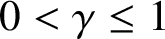$0 < \gamma \leq 1$ ). Lower values of $\gamma $ result in fewer electron jumps, which consequently slows the diffusion process [Reference Benkstein, Kopidakis, van de Lagemaat and Frank5].

In this paper, we employ the Caputo fractional derivative [Reference Caputo8] for its easy adoption of traditional boundary conditions [Reference Garrappa, Kaslik and Popolizio15, Reference Maldon, Lamichhane and Thamwattana27]. Langlands et al. [Reference Langlands, Henry and Wearne20] noted that the use of the Riemann–Liouville fractional derivative leads to an FPDE that is not positivity preserving (see also the article by Baeumer et al. [Reference Baeumer, Kovács, Meerschaert and Sankaranarayanan4]). Without a spatially dependent source term, Langlands et al. [Reference Langlands, Henry and Wearne20] suggested the alternative FPDE

$$ \begin{align*} \frac{\partial n}{\partial t} = D_0 e^{-kt}\frac{\partial^{1 - \gamma} }{\partial t^{1 - \gamma}}\bigg(e^{kt}\frac{\partial^{2} n}{\partial x^{2}}\bigg) - kn, \end{align*} $$

where k is the reaction coefficient. For other fractional reaction–diffusion equations featuring the Riemann–Liouville derivative and the influence of chemical reactions, we refer the reader to the work of Méndez et al. [Reference Méndez, Fedotov and Horsthemke30, Section 3.4]. We also refer the reader to the paper by Meerschaert and Sikorskii [Reference Meerschaert and Sikorskii29, Ch. 7] for the Langlands model, which is another model to study CTRW motion.

The diode equation is commonly used to compute the current–density relationship for solar cells, in which the current J as a function of bias voltage $V_{B}$ is given by [Reference Södergren, Hagfeldt, Olsson and Lindquist36]

$$ \begin{align*} J(V_{B}) = J_{\text{sc}} - J_{0}(e^{qV_{B}/m_{I} k_{B} T - 1}), \end{align*} $$

where $J_{0}$ is the dark saturation current density, given by

$$ \begin{align*} J_{0} = qn_{\text{eq}}\sqrt{D_{0}k_{R}}\tanh\bigg(\!\sqrt{\frac{k_{R}}{D_{0}}} d\bigg). \end{align*} $$

To compute the short-circuit current density $J_{\text {sc}}$ , we use

$$ \begin{align*} J_{\text{sc} }= qD_{0}\bigg[\frac{\partial^{1 - \gamma} }{\partial t^{1 - \gamma}}\bigg(\frac{\partial n}{\partial x}\bigg)\bigg]\bigg|_{x = 0}, \end{align*} $$

noting that the usual electron flux is recovered in the linear diffusion special case $\gamma = 1$ .

Given that the open-circuit voltage $V_{\text {oc}}$ satisfies 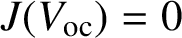$J(V_{\text {oc}}) = 0$ , we may compute the open-circuit voltage with

$$ \begin{align*} V_{\text{oc}} = \frac{m_{I} k_{B} T}{q}\ln\bigg(\frac{J_{\text{sc}}}{J_0} + 1\bigg). \end{align*} $$

Maximizing the power output $P(V_{B}) = V_{B}J(V_{B})$ over $V_{B}$ , we obtain the maximum power point $V_{\max }$ by

$$ \begin{align*} V_{\max} = \frac{m_{I}k_{B}T}{q}\bigg( W\bigg(e\frac{J_{\text{sc}} + J_0}{J_0}\bigg) - 1\bigg), \end{align*} $$

where W is the Lambert W-function [Reference Maldon, Lamichhane and Thamwattana27] and $J_{\max } = J(V_{\max })$ . With $P_{\max } = V_{\max }J_{\max }$ , we compute the efficiency $\eta $ of the DSSC by

(2.5) $$ \begin{align} \eta = \frac{P_{\max}}{P_{i}}, \end{align} $$

where $P_{i}$ is the power of incident light.

In this paper, we use parameter values presented in Table 1 to numerically solve equation (2.1) unless otherwise stated.

Table 1

Parameter values for the numerical simulation.

3 Numerical methods

Let $t_f> 0$ be the final simulation time. Discretizing $[0, t_f]$ into $N_t$ temporal nodes and $[0, d]$ into $N_x$ spatial nodes, we let

$$ \begin{align*}\Delta x = \frac{d}{N_x - 1}, \quad \Delta t = \frac{t_f}{N_t - 1}, \quad x_k = (k - 1)\Delta x , \quad t_m = (m - 1)\Delta t\end{align*} $$

for each $k = 1,\ldots , N_x + 1$ and $m = 1, \ldots , N_t$ . To numerically estimate the fractional derivative of a function f of order $1 - \gamma $ , we use [Reference O’Regan and Grätzel35]

(3.1) $$ \begin{align} \frac{\partial^{1 - \gamma} f}{\partial t^{1 - \gamma}} \bigg|_{t = t_{m}} = \frac{(\Delta t)^{\gamma - 1}}{\Gamma(\gamma + 1)} \sum_{p = 0}^{m - 2} [(p + 1)^{\gamma} - p^{\gamma}][f(t_{m - p}) - f(t_{m - p - 1})] + \textbf{O}\Delta t, \end{align} $$

where $\Gamma $ denotes the usual Gamma function

$$ \begin{align*} \Gamma(z) = \int_{0}^{\infty} x^{z - 1} e^{-x} dx. \end{align*} $$

The finite-difference approximation given in equation (3.1) provides a first-order estimate for the fractional time derivative [Reference Esen, Ucar, Yagmurlu and Tasbozan13]. By using an implicit finite-difference method to discretize time, we obtain an unconditionally stable numerical solution [Reference Langlands and Henry19]. For a second-order approximation, we refer the reader to the paper by Dimitrov [Reference Dimitrov10].

3.1 Finite-difference method

To solve equation (2.1) under the boundary conditions (2.2)–(2.4), we use a finite-difference method (FDM) to discretize space and equation (3.1) to discretize time. In the literature, Esen et al. [Reference Esen, Ucar, Yagmurlu and Tasbozan13] numerically solved the space–time fractional heat equation. Yuste and Acedo [Reference Yuste and Acedo40] proposed an explicit and conditionally stable FDM scheme using Grünwald–Letnikov discretization for the fractional derivative. Lynch et al. [Reference Lynch, Carreras, del-Castillo-Negrete, Ferreira-Mejias and Hicks24] employed a semi-implicit finite-difference method for solving FPDEs, which outperforms standard explicit methods on stability and accuracy. For further details on the consistency, stability and convergence properties of FDM schemes for numerically solving FPDEs, we refer the reader to Li and Zeng’s review paper [Reference Li and Zeng22]. To account for the Neumann boundary condition at $x = d$ , we also employ a ‘ghost node’ at $x = d + \Delta x$ . Let $y_{m, k}$ denote the numerical solution at 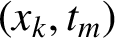$(x_k, t_m)$ . That is,

$$ \begin{align*} n(x_k, t_m) \approx y_{m, k} \end{align*} $$

for each $k = 1, \ldots , N_x + 1$ and $m = 1, \ldots , N_t$ .

3.1.1 Nodes determined by boundary conditions

To satisfy the initial condition (2.4), we set

$$ \begin{align*} y_{1, k} = n_0 \end{align*} $$

for all $k = 1, \ldots , N_x$ . For the Dirichlet boundary condition (2.2) at $x = 0$ , we set

$$ \begin{align*} y_{m, 1} = n_0 \end{align*} $$

for all $m = 1, \ldots , N_t$ . Finally, for the Neumann boundary condition (2.3) at $x = d$ , we use a central difference approximation for the first derivative at $x = d$ to set

$$ \begin{align*} y_{m, Nx + 1} = y_{m, Nx - 1} \end{align*} $$

for all $m = 1,\ldots , N_t$ . Here 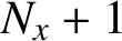$N_x + 1$ corresponds to the ghost node at $x = d + \Delta x$ .

3.1.2 Algorithm

For each $m = 2,\ldots , N_t$ , we set

$$ \begin{align*} \bigg[\frac{\partial n}{\partial t}\bigg]\bigg|_{t = t_m, x = x_k} = D_0\bigg[ \frac{\partial^{1 - \gamma} }{\partial t^{1 - \gamma}}\frac{\partial^{2} n}{\partial x^{2}} \bigg]\bigg|_{t = t_m, x = x_k} + \varphi\alpha e^{-\alpha x_k} - k_R(n(x_k, t_m) - n_{eq}). \end{align*} $$

Using the backward Euler method [Reference Griffiths17], a central difference approximation and equation (3.1) to estimate $\partial {n}/\partial {t}$ , 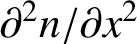$\partial ^2{n}/\partial {x}^{2}$ and the fractional derivative, respectively,

$$ \begin{align*} \frac{y_{m, k} - y_{m - 1, k}}{\Delta t}& = \frac{D_0(\Delta t)^{\gamma - 1}}{\Gamma(\gamma + 1)} \sum_{p = 0}^{m - 2} [(p + 1)^{\gamma} - p^{\gamma}] \\ &\quad \times\bigg[\frac{y_{m - p, k - 1} - 2y_{m - p, k} + y_{m - p, k + 1}}{(\Delta x)^2} - \frac{y_{m - p - 1, k - 1} - 2y_{m - p - 1, k} + y_{m - p - 1, k + 1}}{(\Delta x)^2}\bigg] \\ &\quad + \varphi\alpha e^{-\alpha x_k} - k_R(n(x_k, t_m) - n_{eq}). \end{align*} $$

Upon simplification,

$$ \begin{align*} & -\frac{D_0(\Delta t)^{\gamma}}{\Gamma(\gamma + 1)(\Delta x)^2}y_{m, k - 1} + \bigg[1 + k_R\Delta t + \frac{2D_0(\Delta t)^{\gamma}}{\Gamma(\gamma + 1)(\Delta x)^2}\bigg]y_{m, k} - \frac{D_0(\Delta t)^{\gamma}}{\Gamma(\gamma + 1)(\Delta x)^2}y_{m, k + 1} \\ & \quad = -\frac{D_0(\Delta t)^{\gamma}}{\Gamma(\gamma + 1)(\Delta x)^2}[y_{m - 1, k - 1} - 2y_{m - 1, k} + y_{m - 1, k + 1}] + \frac{D_0(\Delta t)^{\gamma - 1}}{\Gamma(\gamma + 1)} \sum_{p = 1}^{m - 2} [(p + 1)^{\gamma} - p^{\gamma}] \\ &\qquad \times \bigg[\frac{y_{m - p, k - 1} - 2y_{m - p, k} + y_{m - p, k + 1}}{(\Delta x)^2} - \frac{y_{m - p - 1, k - 1} - 2y_{m - p - 1, k} + y_{m - p - 1, k + 1}}{(\Delta x)^2}\bigg] \\ &\qquad + \varphi\alpha e^{-\alpha x_k} - k_R(n(x_k, t_m) - n_{eq}), \end{align*} $$

which results in 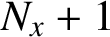$N_x + 1$ equations in 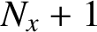$N_x + 1$ unknowns, when combined with the boundary conditions (2.2) and (2.3).

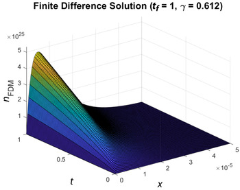
Figure 2 shows the numerical solution to (2.1) under boundary conditions (2.2)–(2.4) using the data from Table 1, 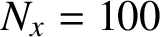$N_x = 100$ , 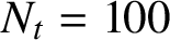$N_t = 100$ and $t_f = 1$ . From Figure 2, we see that the electron density assumes its shape from the interaction of the Dirichlet boundary condition, the exponential source term and diffusion. Note that Figure 2 shows good agreement with the explicit finite-difference method used by Maldon and Thamwattana [Reference Maldon, Lamichhane and Thamwattana27] while significantly improving stability with the use of an implicit finite-difference method.

Figure 2

Plot of the numerical solution to equation (2.1) under (2.2)–(2.4) using the FDM scheme.

3.2 Finite-element method

We also solve equation (2.1) under (2.2)–(2.4) using a finite-element method (FEM) adapted from Alberty et al. [Reference Alberty, Carstensen and Funken1]. Esen et al. [Reference Esen, Ucar, Yagmurlu and Tasbozan13] provided a finite-element basis for the time-fractional diffusion equation under Dirichlet boundary conditions. Yuan and Chen [Reference Yuan and Chen39] solved a mixed diffusion problem featuring the two-sided Riemann–Liouville fractional derivatives by an FEM scheme. Li and Wang [Reference Li and Wang21] solved time-fractional reaction–diffusion and diffusion-wave equations, using Galerkin FEM schemes [Reference Thomée37] which enjoy unconditional stability.

3.2.1 Weak formulation

Letting $\rho = n - n_0$ , we solve the equivalent problem

(3.2) $$ \begin{align} \frac{\partial \rho}{\partial t} = D_0 \frac{\partial^{1 - \gamma} }{\partial t^{1 - \gamma}}\frac{\partial^{2} \rho}{\partial x^{2}} + \varphi\alpha e^{-\alpha x} - k_R(\rho + n_0 - n_{eq}), \end{align} $$

subject to

$$ \begin{align*} \rho(x, 0) &= 0, \\ \rho(0, t) &= 0, \\ \frac{\partial \rho}{\partial x}\bigg|_{x = d} &= 0. \end{align*} $$

Upon multiplying by a test function w and integrating over $[0, d]$ ,

$$ \begin{align*} \int_{0}^{d} \frac{\partial \rho}{\partial t}w \,dx &= D_0 \int_{0}^{d} \frac{\partial^{1 - \gamma} }{\partial t^{1 - \gamma}}\frac{\partial^{2} \rho}{\partial x^{2}}w\, dx \\ &\quad + \int_{0}^{d} (\varphi\alpha e^{-\alpha x} -k_R(n_0 - n_{eq}))w\, dx - k_R \int_{0}^{d} \rho \,w\, dx. \end{align*} $$

Integrating by parts and using the commutativity of the Caputo derivative,

$$ \begin{align*} \int_{0}^{d} \frac{\partial^{1 - \gamma} }{\partial t^{1 - \gamma}}\frac{\partial^{2} \rho}{\partial x^{2}}w \,dx = \bigg[\frac{\partial^{1 - \gamma} }{\partial t^{1 - \gamma}}\bigg(\frac{\partial \rho}{\partial x}\bigg)w\bigg]_{0}^{d} - \int_{0}^{d} \frac{\partial^{1 - \gamma} }{\partial t^{1 - \gamma}}\frac{\partial \rho}{\partial x}\frac{d w}{d x} dx. \end{align*} $$

Given that 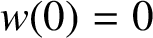$w(0) = 0$ and $({\partial \rho }/{\partial x})|_{x = d} = 0$ , the weak formulation for equation (3.2) is given by

$$ \begin{align*} \int_{0}^{d} \frac{\partial \rho}{\partial t}w \,dx &= -D_0 \int_{0}^{d} \frac{\partial^{1 - \gamma} }{\partial t^{1 - \gamma}}\frac{\partial \rho}{\partial x}\frac{\partial w}{\partial x} \,dx \\ &\quad + \int_{0}^{d} (\varphi\alpha e^{-\alpha x} -k_R(n_0 - n_{eq}))w \,dx - k_R \int_{0}^{d} \rho \,w \,dx. \end{align*} $$

To solve equation (3.2) using this weak formulation, we employ the basis $\{\phi _1, \phi _2, \ldots , \phi _{N_x - 1} \}$ , where $\phi _j$ is given by

$$ \begin{align*} \phi_j(x) = \begin{cases} \dfrac{x - x_{j}}{\Delta x}\quad& x_{j} < x \leq x_{j + 1}, \\[6pt] \dfrac{x_{j + 2} - x}{\Delta x}\quad& x_{j + 1} < x \leq x_{j + 2}, \\ 0\quad& \text{otherwise}, \end{cases} \end{align*} $$

for $j = 1, \ldots , N_x - 2$ and $\phi _{N_x - 1}$ is given by

$$ \begin{align*} \phi_{N_x - 1}(x) = \begin{cases} \dfrac{x - x_{N_x - 1}}{\Delta x}\quad& x_{N_x - 1} < x \leq d, \\ 0\quad& \text{otherwise}. \end{cases} \end{align*} $$

3.3 Algorithm

At each time step $t_m$ , we set

$$ \begin{align*} \rho(x, t_m) \approx P(x, t_m) \sum_{j = 1}^{N_x - 1} g_{j}(t_m)\phi_j(x), \end{align*} $$

where $g_{j}$ are the coefficients of the basis functions. In matrix form, the weak formulation of equation (3.2) under the basis $\{\phi _1, \phi _2, \ldots , \phi _{N_x - 1} \}$ is given by

$$ \begin{align*} M\frac{\partial \vec{g}}{\partial t} = -D_0 A \frac{d^{1 - \gamma} \vec{g}}{d {t}^{1 - \gamma}} - k_R M\vec{g} + \vec{C}, \end{align*} $$

where the coefficient vector $\vec {g}$ , the mass matrix M, the stiffness matrix A and the load vector $\vec {C}$ components are given by

$$ \begin{align*} \vec{g}_m &= [g_1(t_m), g_2(t_m), \ldots, g_{N_x - 1}(t_m) ], \\ M_{i, j} &= \int_{0}^{d} \phi_i(x)\phi_j(x) \,dx, \\ A_{i, j} &= \int_{0}^{d} \frac{d \phi_i}{d x}\frac{d \phi_j}{d x}\, dx, \\ \vec{C}_j &= \int_{0}^{d} [\varphi\alpha e^{-\alpha x} - k_R(n_0 - n_{eq})]\phi_j(x) \,dx \end{align*} $$

for each $m = 1, \ldots , N_t$ , $i = 1,\ldots , N_x - 1$ and $j = 1, \ldots , N_x - 1$ . Applying the implicit finite-difference method to discretize time, we obtain the system

$$ \begin{align*} A_L \vec{g}_m = A_c \vec{g}_{m - 1} + A_R \sum_{p = 1}^{m - 2} [(p + 1)^{\gamma} - p^{\gamma}][\vec{g}_{m - p} - \vec{g}_{m - p - 1}] + \Delta t\vec{C}, \end{align*} $$

where

$$ \begin{align*} A_L &= (1 + k_R\Delta t)M + \frac{D_0(\Delta t)^{\gamma}}{\Gamma(\gamma + 1)}A, \\ A_C &= k_R(\Delta t)M + \frac{D_0(\Delta t)^{\gamma}}{\Gamma(\gamma + 1)}A, \\ A_R &= -\frac{D_0(\Delta t)^{\gamma}}{\Gamma(\gamma + 1)}A. \end{align*} $$

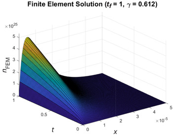
Figure 3 shows the numerical solution to equation (2.1) under the conditions (2.2)–(2.4) using the data from Table 1, 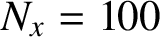$N_x = 100$ , 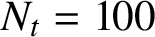$N_t = 100$ and $t_f = 1$ .

Figure 3

Plot of the numerical solution to equation (2.1) under (2.2)–(2.4) using the finite-element method.

4 Efficiency calculations

To elucidate the effect of the $\text {TiO}_2$ nanoporous semiconductor on efficiency through the parameter $\gamma $ , we calculate $\eta $ using equation (2.5) and the numerical solution obtained by the finite-difference method.

4.1 Electron flux calculation

To calculate the short-circuit current density, we estimate the time-fractional derivative with equation (3.1) and the electron flux at $x = 0$ with the $10$ -point estimate from Maldon and Thamwattana [Reference Maldon, Lamichhane and Thamwattana27]. Therefore, under the finite-difference method the short-circuit current density is given by

$$ \begin{align*} J_{\text{sc} }= \frac{qD_0(\Delta t)^{\gamma - 1}}{\Gamma(\gamma + 1)}\sum_{p = 0}^{N_t - 2} [(p + 1)^{\gamma} - p^{\gamma}]\bigg[\sum_{j = 1}^{10} a_j(y_{N_t - p, j} - y_{N_t - p - 1, j})\bigg], \end{align*} $$

where each coefficient is given by

$$\begin{align*}\begin{array}{clll} &a_1 = -\dfrac{7129}{2520\Delta x}, &a_2 = \dfrac{9}{\Delta x}, & a_3 = -\dfrac{18}{\Delta x}, \\[6pt] &a_4 = \dfrac{28}{\Delta x}, &a_5 = -\dfrac{63}{2\Delta x}, & a_6 = \dfrac{126}{5\Delta x}, \\[6pt] &a_7 = -\dfrac{14}{\Delta x}, &a_8 = \dfrac{36}{7\Delta x}, & a_9 = -\dfrac{9}{8\Delta x}, \quad a_{10} = \dfrac{1}{9\Delta x}. \end{array}\end{align*}$$

4.1.1 Efficiency calculations

In Table 2, we calculate the efficiency $\eta $ under several values for the parameter $\gamma $ and the numerical data provided in Table 1. From the table, we see that efficiency decreases as $\gamma $ increases, which is indicative of longer waiting times in the CTRW simulation [Reference Maldon, Lamichhane and Thamwattana27].

Table 2

Values for efficiency $\eta $ (%) under several values of the parameter $\gamma $ .

Table 3

Errors for the finite-difference method (FDM) and finite-element method (FEM) for solving equation (2.1) under temporal refinement given $N_x = 100$ , using equation (5.1).

Table 4

Errors for the finite-difference method (FDM) and finite-element method (FEM) for solving equation (2.1) under spatial refinement given $N_t = 1000$ , using equation (5.1).

5 Error calculation

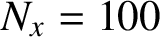
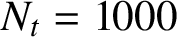
In lieu of an analytical solution, we compute the accuracy of each method using a comparison to a fine grid solution from the same numerical method. We calculate the errors for $t_f = 1$ under the parameter data in Table 1. For the reference solution, we use a finite-difference solution and finite element with $1000$ spatial nodes and $1000$ temporal nodes.

To calculate the error $\epsilon $ for both schemes under refinement, we use

(5.1) $$ \begin{align} \epsilon = \frac{\sqrt{\Delta x\Delta t}}{n_0}|| \vec{u}_{C} - \vec{u}_{F} ||, \end{align} $$

where $\vec {u}_C$ is the coarse grid solution vector, $\vec {u}_{F}$ is the interpolated fine grid solution vector, $\Delta x$ and $\Delta t$ are calculated in the coarse grid and $||\cdot ||$ denotes the usual root-mean-square error. We scale $\epsilon $ by $n_0^{-1}$ to account for the high magnitude of the numerical solution.

From Table 3, we see that the error decreases by a factor of two when the number of temporal nodes doubles, which confirms that equation (3.1) provides a first-order approximation for the fractional time derivative in equation (2.1) for both numerical schemes. Table 4 shows that the error for both schemes decreases by a factor of four when the number of spatial nodes doubles, confirming that the finite-difference method and finite-element method provide second-order spatial discretizations. From Tables 3 and 4, we see that the finite-element scheme is consistently more accurate than the finite-difference scheme, since the weak formulation of the finite-element method naturally satisfies the Dirichlet and Neumann boundary conditions.

6 Summary

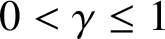
We solve the fractional partial differential equation (2.1) using a finite-difference method and a finite-element method to discretize space and an implicit finite-difference method to discretize time. Our numerical results are in good agreement with the literature. Error analysis indicates that the finite-difference method and finite-element method feature respectively first- and second-order spatial approximations while equation (3.1) provides an unconditionally stable finite- difference approximation for Caputo fractional derivatives of order $0 < \gamma \leq 1$ .

Finally, we use the numerical schemes to compute the efficiency of a DSSC under several values of $\gamma $ to elucidate the effect of electron diffusion in the nanoporous semiconductor. We find that lower values of $\gamma $ lead to lower efficiencies due to the slower diffusion process associated with longer waiting times in the CTRW simulation.