1 Introduction
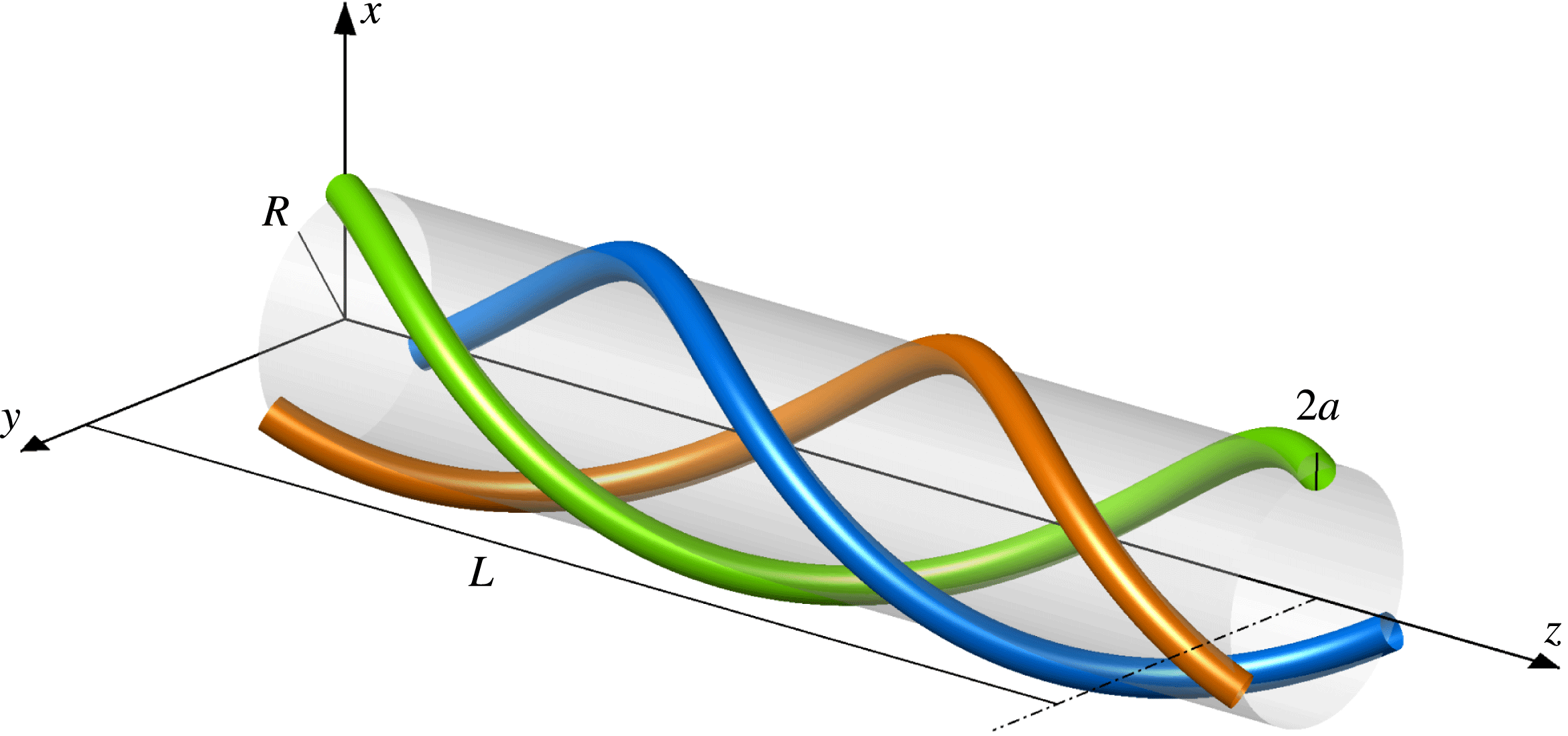
A set of equal coaxial symmetrically located helical vortices (figure 1) moving in an unbounded inviscid incompressible fluid approximates the tip vortices in the far wakes of multibladed wind turbines, propellers or rotors. Joukowsky (Reference Joukowsky1912) deduced that this ideal set translates and rotates steadily while the vortices preserve their form and relative position. He found the approximate velocity of a single vortex but did not pursue the analysis for two or more vortices. While there have been numerous attempts to determine the motion of a single helical vortex (for a brief summary of previous contributions, see, e.g., Velasco Fuentes Reference Velasco Fuentes2018), to the best of our knowledge, only Wood & Boersma (Reference Wood and Boersma2001), Okulov (Reference Okulov2004) and Okulov & Sørensen (Reference Okulov and Sørensen2007) have attempted to determine the motion of multiple helical vortices. They calculated the velocity of the vortices by adding the self-induced velocity, defined as the velocity that the
 $i$
th vortex would have in an otherwise quiescent fluid, to the mutually induced velocity, defined as the velocity induced by the remaining
 $N-1$
vortices on the
 $i$
th vortex. Unfortunately, Wood & Boersma (Reference Wood and Boersma2001) and Okulov & Sørensen (Reference Okulov and Sørensen2007) neglected the tangential components and computed the binormal components only; Okulov (Reference Okulov2004), on the other hand, computed the total velocity but made an error in the analysis of the self-induced velocity (Velasco Fuentes Reference Velasco Fuentes2018).
Segments of three thin helical vortices of cross-sectional radius
 $a$
. The vortices extend indefinitely in both directions and their centrelines are helices of pitch
 $L$
and radius
 $R$
lying on the surface of an imaginary supporting cylinder.

The first objective of this paper is therefore to write down explicit formulae for the velocities of the vortices as functions of the number of vortices and of their pitch and cross-sectional radius. We do this in § 2 by adding the mutually induced velocities found by Okulov (Reference Okulov2004) to the self-induced velocities found by Velasco Fuentes (Reference Velasco Fuentes2018). In § 3, we verify our results by numerically computing the velocities using the Helmholtz integral and the Rosenhead–Moore approximation to the Biot–Savart law, as well as numerical simulations of the evolution of the vortices under the Euler equations in a triple-periodic box.
Besides the motion of the vortices themselves, the velocity field that they induce has also attracted the attention of researchers from an early stage. Although Kelvin (Reference Thomson1875) was discussing a slightly different problem, namely vortices coiled on a torus instead of a cylinder, it is illustrative to quote him: ‘The setting forth of (the electromagnetic) analogy to people
 $(\ldots )$
familiar with the distribution of magnetic force in the neighbourhood of an electric circuit, does much to promote a clear understanding of the still somewhat strange fluid motions with which we are at present occupied.’ Only recently, it was shown just how ‘strange’ the fluid motion is in this case: the streamlines are chaotic (Velasco Fuentes Reference Velasco Fuentes2010; Velasco Fuentes & Romero Arteaga Reference Velasco Fuentes and Romero Arteaga2011). The electromagnetic analogy also enabled Fitzgerald (Reference Fitzgerald1899) to speculate about the flow induced by a helical vortex: ‘There will be, on the whole, a flow along the inside of the spiral, but the motion of the fluid is complex.’ It is worth mentioning that Lamb (Reference Lamb1923) calculated the magnetic field produced by a constant current through a helical wire, which amounts to computing the velocity field induced by a helical vortex. He, however, did not mention this interpretation and this work has remained largely unnoticed by the fluid dynamics community. Kawada (Reference Kawada1939) studied a problem similar to the one we are dealing with: the velocity field of a set of helical vortices plus a rectilinear vortex on the axis. He succeeded in computing the velocity field and used the electromagnetic analogy to verify (albeit qualitatively) his results. Finally, Hardin (Reference Hardin1982) obtained the velocity field produced by an infinitely thin helical vortex. This result has been widely used to compute the velocity of the vortex itself (see, e.g., Ricca Reference Ricca1994; Boersma & Wood Reference Boersma and Wood1999; Okulov Reference Okulov2004; Okulov & Sørensen Reference Okulov and Sørensen2007; Velasco Fuentes Reference Velasco Fuentes2018). Mezić, Leonard & Wiggins (Reference Mezić, Leonard and Wiggins1998) and Andersen & Brøns (Reference Andersen and Brøns2014) studied the topology of Hardin’s velocity field in a system translating and rotating with the vortex, taking into account the binormal component of the vortex motion only.
The main objective of this paper is to characterize the motion of passive particles in the velocity field of a set of coaxial helical vortices and, in particular, to determine the capacity of the set of vortices to transport fluid. In § 4, we do this by analysing the topology of the velocity field induced by the vortices in a system that moves with the vortices; i.e. in a system that translates with the linear velocity (
 $U$
) and rotates with the angular velocity (
 $\unicode[STIX]{x1D6FA}$
) obtained in § 2.
2 Vortex motion
Helical vortices are thin tubes of infinite length whose centrelines are mathematical helices, i.e. curves of constant curvature and torsion (see figure 1). The centreline of the
 $i$
th vortex is given, in Cartesian coordinates, as follows:
 $$\begin{eqnarray}\left.\begin{array}{@{}c@{}}x_{i}=R\cos (\unicode[STIX]{x1D703}-2\unicode[STIX]{x03C0}\text{i}/N),\\ y_{i}=R\sin (\unicode[STIX]{x1D703}-2\unicode[STIX]{x03C0}\text{i}/N),\\ z_{i}=L\unicode[STIX]{x1D703}/2\unicode[STIX]{x03C0},\end{array}\right\}\end{eqnarray}$$
where
 $\unicode[STIX]{x1D703}$
is the angle around the axis of the imaginary supporting cylinder,
 $R$
is the radius of this cylinder,
 $L$
is the pitch of the helix and
 $N$
is the number of vortices.
Each vortex has a circular cross-section (of radius
 $a$
) where the vorticity is uniform and parallel to the centreline. The circulation of all vortices is the same (
 $\unicode[STIX]{x1D6E4}$
) and the
 $z$
-component of their vorticity is always in the positive
 $z$
direction (see figure 1). The circular shape as well as the uniform vorticity are leading-order approximations only: in a steady solution of the Euler equations, the vorticity varies linearly with the distance from the centre of curvature and the cross-section slightly differs from a circle.
The centrelines of the vortices intersect any polar plane (
 $z=z_{0}$
) on the vertices of a regular polygon of
 $N$
sides inscribed in a circle of radius
 $R$
. Therefore, the flow evolution is determined by three non-dimensional parameters only: the number of vortices
 $N$
, the vortex radius
 $\unicode[STIX]{x1D6FC}=a/R$
and the vortex pitch
 $\unicode[STIX]{x1D70F}=L/2\unicode[STIX]{x03C0}R$
.
It is worth mentioning that the values of the pitch and the radius of the vortices cannot be chosen arbitrarily. A cursory glance may suggest that the pitch of a single helical vortex can be as small as twice its radius, i.e.
 $L\geqslant 2a$
in dimensional form. However, results obtained for an infinite row of Rankine vortices indicate that the vortex must satisfy
 $L\geqslant 4a$
if it is to avoid erosion or even destruction. Considering multiple vortices and dimensionless variables, this translates into the following condition:
 $\unicode[STIX]{x1D70F}\geqslant 2N\unicode[STIX]{x1D6FC}/\unicode[STIX]{x03C0}$
.
We determine the motion of the vortices by adding the self-induced velocity, defined as the velocity that the
 $i$
th vortex would have in an otherwise quiescent fluid, to the mutually induced velocity, defined as the velocity induced by the remaining
 $N-1$
vortices on the
 $i$
th vortex. Therefore, the set of vortices has linear velocity
 $U=U_{S}+U_{M}$
and angular velocity
 $\unicode[STIX]{x1D6FA}=\unicode[STIX]{x1D6FA}_{S}+\unicode[STIX]{x1D6FA}_{M}$
, where the subscripts
 $S$
and
 $M$
indicate self- and mutually induced velocity respectively. To obtain
 $U_{S}$
and
 $\unicode[STIX]{x1D6FA}_{S}$
, Velasco Fuentes (Reference Velasco Fuentes2018) evaluated the velocity field at two diametrically opposed points on the vortex boundary using the approximation of Boersma & Wood (Reference Boersma and Wood1999) to the velocity field of Hardin (Reference Hardin1982). In dimensionless form, the self-induced velocities are
 $$\begin{eqnarray}\displaystyle & \displaystyle U_{S}^{\ast }={\displaystyle \frac{1}{(1+\unicode[STIX]{x1D70F}^{2})^{3/2}}}\ln \left({\displaystyle \frac{2}{\unicode[STIX]{x1D716}\sqrt{1+\unicode[STIX]{x1D70F}^{2}}}}\right)+W(\unicode[STIX]{x1D70F}), & \displaystyle\end{eqnarray}$$
 $$\begin{eqnarray}\displaystyle & \displaystyle \unicode[STIX]{x1D6FA}_{S}^{\ast }={\displaystyle \frac{-\unicode[STIX]{x1D70F}}{(1+\unicode[STIX]{x1D70F}^{2})^{3/2}}}\left[\ln \left({\displaystyle \frac{2}{\unicode[STIX]{x1D716}\sqrt{1+\unicode[STIX]{x1D70F}^{2}}}}\right)+2(1+\unicode[STIX]{x1D70F}^{2})\right]-\unicode[STIX]{x1D70F}W(\unicode[STIX]{x1D70F})+2, & \displaystyle\end{eqnarray}$$
where
 $\unicode[STIX]{x1D716}=a/R(1+\unicode[STIX]{x1D70F}^{2})$
and
 $W(\unicode[STIX]{x1D70F})$
is an integral defined by Boersma & Wood (Reference Boersma and Wood1999). They believed that
 $W(\unicode[STIX]{x1D70F})$
could not be evaluated in closed form so they computed it numerically and obtained asymptotic forms for small and large values of
 $\unicode[STIX]{x1D70F}$
. Okulov (Reference Okulov2004) calculated the following approximation:
 $$\begin{eqnarray}\displaystyle W(\unicode[STIX]{x1D70F}) & {\approx} & \displaystyle {\displaystyle \frac{1}{\sqrt{1+\unicode[STIX]{x1D70F}^{2}}}}-{\displaystyle \frac{1}{t}}+{\displaystyle \frac{1}{(1+\unicode[STIX]{x1D70F}^{2})^{3/2}}}\left[\ln \left({\displaystyle \frac{t}{2(1+\unicode[STIX]{x1D70F}^{2})}}\right)-2\unicode[STIX]{x1D70F}^{2}\right]-{\displaystyle \frac{4}{\unicode[STIX]{x1D70F}^{2}}}\text{I}_{1}\left({\displaystyle \frac{1}{\unicode[STIX]{x1D70F}}}\right)\text{K}_{1}^{\prime }\left({\displaystyle \frac{1}{\unicode[STIX]{x1D70F}}}\right)\nonumber\\ \displaystyle & & \displaystyle +\,{\displaystyle \frac{t^{2}}{(1+\unicode[STIX]{x1D70F}^{2})^{9/2}}}\left[\left(\unicode[STIX]{x1D70F}^{4}-3\unicode[STIX]{x1D70F}^{2}+{\displaystyle \frac{3}{8}}\right)\unicode[STIX]{x1D701}(3)-2\unicode[STIX]{x1D70F}^{4}-{\displaystyle \frac{27}{8}}-{\displaystyle \frac{1}{\unicode[STIX]{x1D70F}^{2}}}\right],\end{eqnarray}$$
where
 $\unicode[STIX]{x1D701}(3)\approx 1.20206$
is the Riemann zeta function,
 $\text{K}_{1}$
and
 $\text{I}_{1}$
are modified Bessel functions and the prime indicates a derivative with respect to the argument. This approximation leads to errors in the velocity of up to 0.5 % (with a mean of 0.004 %) in the region of the parameter space shown in figure 2. In this paper, we compute
 $W(\unicode[STIX]{x1D70F})$
using the numerical method described by Boersma & Wood (Reference Boersma and Wood1999).
Okulov (Reference Okulov2004) obtained
 $U_{M}$
and
 $\unicode[STIX]{x1D6FA}_{M}$
by a complicated but efficient procedure to evaluate the Kapteyn-like series appearing in the velocity field of Hardin (Reference Hardin1982). In dimensionless form, and after correcting the misprinted sign of the third term in the formula for
 $\unicode[STIX]{x1D6FA}_{M}$
, the mutually induced velocities are
 $$\begin{eqnarray}\displaystyle U_{M}^{\ast } & = & \displaystyle {\displaystyle \frac{2N-2-\unicode[STIX]{x1D6FA}_{M}^{\ast }}{\unicode[STIX]{x1D70F}}},\end{eqnarray}$$
 $$\begin{eqnarray}\displaystyle \unicode[STIX]{x1D6FA}_{M}^{\ast } & = & \displaystyle N-3+{\displaystyle \frac{\unicode[STIX]{x1D70F}}{(1+\unicode[STIX]{x1D70F}^{2})^{3/2}}}(\log (N)-1)-{\displaystyle \frac{4}{\unicode[STIX]{x1D70F}}}\text{I}_{1}\left({\displaystyle \frac{1}{\unicode[STIX]{x1D70F}}}\right)\text{K}_{1}^{\prime }\left({\displaystyle \frac{1}{\unicode[STIX]{x1D70F}}}\right)\nonumber\\ \displaystyle & & \displaystyle +\,{\displaystyle \frac{\unicode[STIX]{x1D70F}^{3}}{(1+\unicode[STIX]{x1D70F}^{2})^{9/2}}}\left[\left(\unicode[STIX]{x1D70F}^{4}-3\unicode[STIX]{x1D70F}^{2}+{\displaystyle \frac{3}{8}}\right)\left({\displaystyle \frac{\unicode[STIX]{x1D701}(3)(N^{2}-1)}{N^{2}}}-1\right)\right].\end{eqnarray}$$
In dimensional form, the velocities of the set of vortices are
 $$\begin{eqnarray}\displaystyle & \displaystyle U={\displaystyle \frac{\unicode[STIX]{x1D6E4}}{4\unicode[STIX]{x03C0}R}}(U_{S}^{\ast }+U_{M}^{\ast }), & \displaystyle\end{eqnarray}$$
 $$\begin{eqnarray}\displaystyle & \displaystyle \unicode[STIX]{x1D6FA}={\displaystyle \frac{\unicode[STIX]{x1D6E4}}{4\unicode[STIX]{x03C0}R^{2}}}(\unicode[STIX]{x1D6FA}_{S}^{\ast }+\unicode[STIX]{x1D6FA}_{M}^{\ast }). & \displaystyle\end{eqnarray}$$
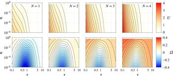
Figure 2 shows
 $U$
and
 $\unicode[STIX]{x1D6FA}$
in the region
 $10^{-6}<\unicode[STIX]{x1D6FC}<0.4$
and
 $0.1<\unicode[STIX]{x1D70F}<10$
for
 $N=1,2,3,4$
vortices. The set of vortices always translates in the direction of the
 $z$
-component of the vorticity (see figure 1); its velocity
 $U$
increases with the number of vortices
 $N$
and decreases as the vortex pitch
 $\unicode[STIX]{x1D70F}$
and vortex radius
 $\unicode[STIX]{x1D6FC}$
increase. The region of the parameter space where the set of vortices rotates in the direction of the
 $xy$
-component of the vorticity (i.e. anticlockwise when seen from the direction in which the set translates) grows with the number of vortices
 $N$
(see the red regions in figure 2). For a fixed radius
 $\unicode[STIX]{x1D6FC}$
, the set rotates with an angular velocity
 $\unicode[STIX]{x1D6FA}$
that has a minimum when their pitch
 $\unicode[STIX]{x1D70F}$
is approximately one. For a fixed pitch
 $\unicode[STIX]{x1D70F}$
, the set rotates with an angular velocity
 $\unicode[STIX]{x1D6FA}$
that decreases with the radius
 $\unicode[STIX]{x1D6FC}$
.
The linear and angular velocities of helical vortices (
 $U$
and
 $\unicode[STIX]{x1D6FA}$
respectively) as functions of the number of vortices (
 $N$
) and their pitch and radius (
 $\unicode[STIX]{x1D70F}$
and
 $\unicode[STIX]{x1D6FC}$
respectively). Positive values of
 $U$
indicate translation in the positive
 $z$
direction of figure 1; positive values of
 $\unicode[STIX]{x1D6FA}$
indicate anticlockwise rotation when the vortices are viewed from the positive
 $z$
direction. The contour interval for
 $U$
is 0.2 and for
 $\unicode[STIX]{x1D6FA}$
is 0.02.

The binormal and tangential components of the velocities of the vortices may be obtained from
 $U$
and
 $\unicode[STIX]{x1D6FA}$
by a simple frame rotation (see, e.g., Velasco Fuentes Reference Velasco Fuentes2018). Thus, using the linear and angular velocities (2.7)–(2.8) and the approximation of
 $W(\unicode[STIX]{x1D70F})$
given by (2.4), we obtain the binormal and tangential velocities of the vortices,
 $$\begin{eqnarray}\displaystyle U_{b}^{\ast } & = & \displaystyle {\displaystyle \frac{1}{(1+\unicode[STIX]{x1D70F}^{2})^{3/2}}}\left\{\ln \left({\displaystyle \frac{\unicode[STIX]{x1D70F}}{\unicode[STIX]{x1D716}N(1+\unicode[STIX]{x1D70F}^{2})^{3/2}}}\right)\right.\nonumber\\ \displaystyle & & \displaystyle +\,{\displaystyle \frac{\unicode[STIX]{x1D70F}^{2}}{(1+\unicode[STIX]{x1D70F}^{2})^{3}}}\left[\left(\unicode[STIX]{x1D70F}^{4}-3\unicode[STIX]{x1D70F}^{2}+{\displaystyle \frac{3}{8}}\right)\left(1+{\displaystyle \frac{\unicode[STIX]{x1D701}(3)}{N^{2}\unicode[STIX]{x1D70F}^{2}(1+\unicode[STIX]{x1D70F}^{2})^{3/2}}}\right)-2\unicode[STIX]{x1D70F}^{4}-{\displaystyle \frac{27}{8}}-{\displaystyle \frac{1}{\unicode[STIX]{x1D70F}^{2}}}\right]\nonumber\\ \displaystyle & & \displaystyle \left.+\,(1-\unicode[STIX]{x1D70F}^{4})\left({\displaystyle \frac{N}{\unicode[STIX]{x1D70F}}}+{\displaystyle \frac{1}{\sqrt{1+\unicode[STIX]{x1D70F}^{2}}}}\right)+(1+\unicode[STIX]{x1D70F}^{2})^{3/2}+\unicode[STIX]{x1D70F}^{2}\sqrt{1+\unicode[STIX]{x1D70F}^{2}}\right\},\end{eqnarray}$$
 $$\begin{eqnarray}\displaystyle U_{t}^{\ast } & = & \displaystyle {\displaystyle \frac{2(N\sqrt{1+\unicode[STIX]{x1D70F}^{2}}-\unicode[STIX]{x1D70F})}{1+\unicode[STIX]{x1D70F}^{2}}},\end{eqnarray}$$
for a set of
 $N$
helical vortices of pitch
 $\unicode[STIX]{x1D70F}$
and radius
 $\unicode[STIX]{x1D6FC}$
satisfying
 $N>1$
,
 $\unicode[STIX]{x1D6FC}^{2}\ll 1$
and
 $\unicode[STIX]{x1D70F}\geqslant 2N\unicode[STIX]{x1D6FC}/\unicode[STIX]{x03C0}$
. These velocities must be multiplied by
 $\unicode[STIX]{x1D6E4}/4\unicode[STIX]{x03C0}R$
to obtain the dimensional ones.
3 Comparison with numerical results
We verified the analytical results by computing the velocity of the vortex by numerical integration of the Helmholtz formula,
 $$\begin{eqnarray}\boldsymbol{u}(\boldsymbol{x})=-{\displaystyle \frac{1}{4\unicode[STIX]{x03C0}}}\int {\displaystyle \frac{[\boldsymbol{x}-\boldsymbol{x}^{\prime }]\times \unicode[STIX]{x1D74E}}{|\boldsymbol{x}-\boldsymbol{x}^{\prime }|^{3}}}\,\text{d}V,\end{eqnarray}$$
where
 $\unicode[STIX]{x1D74E}$
is the vorticity at
 $\boldsymbol{x}^{\prime }$
, and of the Rosenhead–Moore approximation to the Biot–Savart law,
 $$\begin{eqnarray}\boldsymbol{u}(\boldsymbol{x})=-{\displaystyle \frac{\unicode[STIX]{x1D6E4}}{4\unicode[STIX]{x03C0}}}\int {\displaystyle \frac{[\boldsymbol{x}-\boldsymbol{r}(s)]\times \text{d}\boldsymbol{r}}{(|\boldsymbol{x}-\boldsymbol{r}(s)|^{2}+\unicode[STIX]{x1D707}^{2}a^{2})^{3/2}}},\end{eqnarray}$$
where
 $\boldsymbol{r}(s)$
gives the centerline of the vortex as a function of the arclength
 $s$
and
 $\unicode[STIX]{x1D707}=e^{-3/4}$
(see Saffman Reference Saffman1995).
We evaluated the velocity at
 $(x,y,z)=(R,0,0)$
by integrating (3.1) and (3.2) in the interval
 $-nL<z<nL$
, where
 $n$
is an integer and
 $L$
is the dimensional pitch. In the computation of the Rosenhead–Moore integral, we used one filament per vortex and represented each filament with
 $M$
straight elements per helix coil. In the computation of the Helmholtz integral, we used 100 filaments per vortex and, again, represented each filament with
 $M$
straight elements per helix coil. The value of
 $M$
varied between
 $10^{3}$
and
 $10^{4}$
depending on the helix pitch
 $L$
. We chose
 $n$
large enough to make the difference between the integrals computed with
 $n$
and
 $n+1$
negligible.
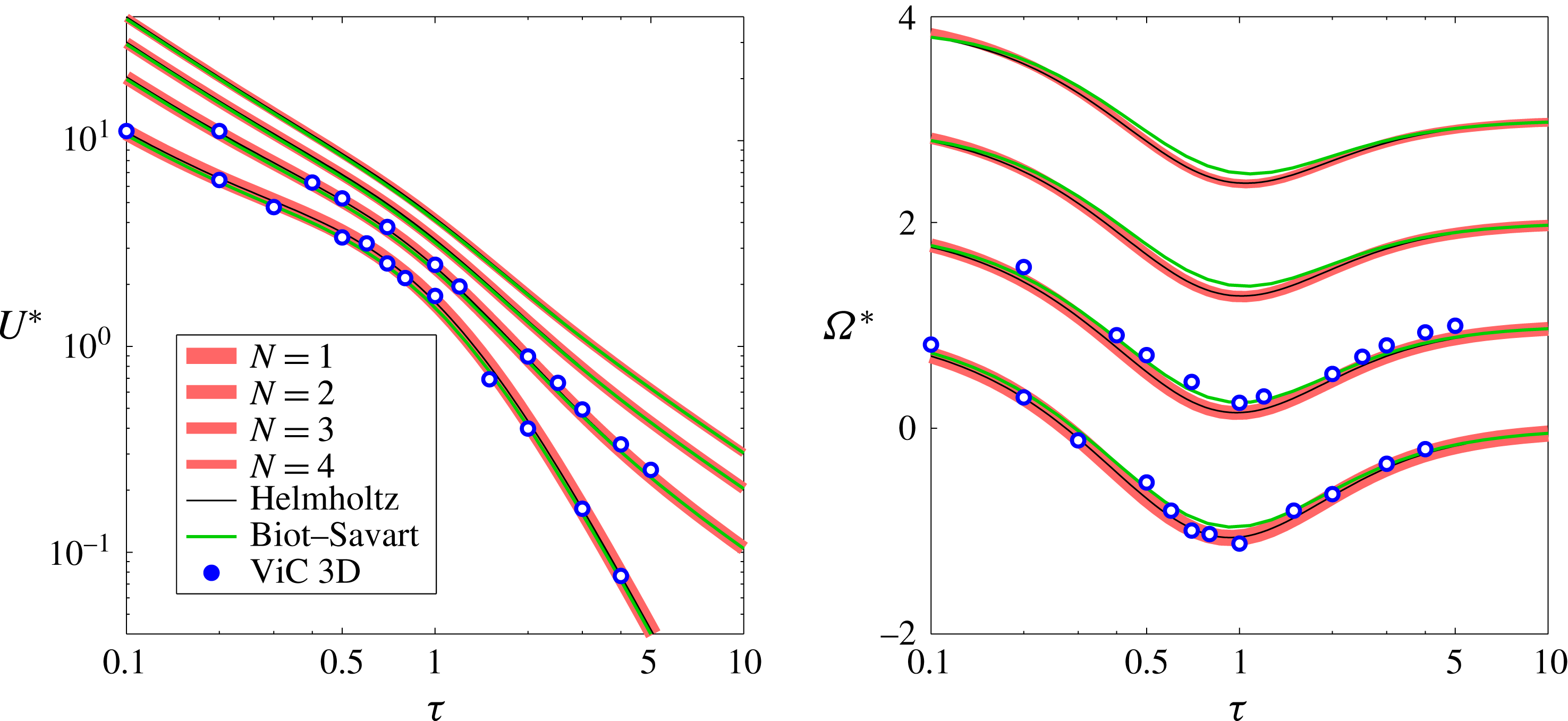
Dimensionless linear and angular velocities,
 $U^{\ast }$
and
 $\unicode[STIX]{x1D6FA}^{\ast }$
respectively, as functions of the number of vortices (
 $N$
) and the vortex pitch (
 $\unicode[STIX]{x1D70F}$
) for a given vortex radius (
 $\unicode[STIX]{x1D6FC}=0.1$
).

Figure 3 shows the dimensionless linear and angular velocities,
 $U^{\ast }$
and
 $\unicode[STIX]{x1D6FA}^{\ast }$
respectively, as functions of the vortex pitch (
 $0.1<\unicode[STIX]{x1D70F}<10$
) for a given vortex radius (
 $\unicode[STIX]{x1D6FC}=0.1$
). There is excellent agreement between the velocities computed with (2.7)–(2.8) and the Helmholtz integral for all values of
 $\unicode[STIX]{x1D70F}$
and
 $N$
. The agreement between the theoretical velocities and the velocities obtained with the Rosenhead–Moore approximation is also very good, except for
 $\unicode[STIX]{x1D6FA}^{\ast }$
around
 $\unicode[STIX]{x1D70F}=1$
, where the relative differences reach approximately 5 % for all values of
 $N$
.
We also verified our theoretical results by computing the motion of the vortices using a three-dimensional vortex-in-cell model that solves the vorticity equation for an incompressible homogeneous fluid. A sketch of the method is given below; for a more detailed description, see, e.g., Suaza Jaque & Velasco Fuentes (Reference Suaza Jaque and Velasco Fuentes2017) and references therein. First, each tubular vortex is discretized as a set of labelled particles with a vorticity
 $\unicode[STIX]{x1D74E}_{n}$
. Then, the vorticity of the particles is interpolated onto a regular grid using a bi-quadratic scheme. From this vorticity field, the velocity potential
 $\boldsymbol{A}$
is obtained by solving the Poisson equation
 $\unicode[STIX]{x1D6FB}^{2}\boldsymbol{A}=-\unicode[STIX]{x1D74E}$
with a complex fast Fourier transform routine; then, the velocity field is computed by differentiating the potential,
 $\boldsymbol{u}=\unicode[STIX]{x1D735}\times \boldsymbol{A}$
. The new positions and vorticities of the particles are obtained by integrating the equations
 $\text{d}\boldsymbol{x}_{n}/\text{d}t=\boldsymbol{u}$
and
 $\text{d}\unicode[STIX]{x1D74E}_{n}/\text{d}t=\unicode[STIX]{x1D74E}\boldsymbol{\cdot }\unicode[STIX]{x1D735}\boldsymbol{u}$
using a second-order Runge–Kutta scheme after the Eulerian quantities on the right-hand side have been interpolated back to the particles.
We determined
 $U$
and
 $\unicode[STIX]{x1D6FA}$
for a given initial condition by calculating the linear and angular displacements of individual labelled particles, dividing those displacements by the elapsed time and taking the average over all particles (2–5
 $\times 10^{5}$
). Figure 3 shows that the results for
 $N=1,2$
agree well with the theoretical velocities.
4 Flow topology
In this section, we use the helical stream function introduced by Hardin (Reference Hardin1982) and analyse its topology in a reference frame where the vortices are stationary; that is to say, in a frame that translates with linear velocity
 $U$
and rotates with angular velocity
 $\unicode[STIX]{x1D6FA}$
. We do this because, in a co-moving frame, particle trajectories coincide with streamlines; it is, therefore, the only frame where the topology of the stream function provides information about the capacity of the vortices to carry fluid.
The steady stream function
 $\unicode[STIX]{x1D6F9}$
is
 $$\begin{eqnarray}\unicode[STIX]{x1D6F9}(r,\unicode[STIX]{x1D719})={\displaystyle \frac{1}{2}}\left(\unicode[STIX]{x1D6FA}-{\displaystyle \frac{U}{l}}\right)r^{2}+\mathop{\sum }_{i=1}^{N}\unicode[STIX]{x1D713}_{i}(r,\unicode[STIX]{x1D719}),\end{eqnarray}$$
where
 $l=L/2\unicode[STIX]{x03C0}$
,
 $(r,\unicode[STIX]{x1D719})$
are helical coordinates, related to the cylindrical coordinates by
 $(r,\unicode[STIX]{x1D719})=(r,\unicode[STIX]{x1D703}-z/l)$
, and
 $\unicode[STIX]{x1D713}_{i}$
is the stream function corresponding to the
 $i$
th vortex, defined as follows (Hardin Reference Hardin1982):
 $$\begin{eqnarray}\unicode[STIX]{x1D713}_{i}(r,\unicode[STIX]{x1D719})=\left\{\begin{array}{@{}ll@{}}{\displaystyle \frac{\unicode[STIX]{x1D6E4}(r^{2}-R^{2})}{4\unicode[STIX]{x03C0}l^{2}}}-{\displaystyle \frac{\unicode[STIX]{x1D6E4}Rr}{\unicode[STIX]{x03C0}l^{2}}}S_{1}(r,\unicode[STIX]{x1D719}-2\unicode[STIX]{x03C0}\text{i}/N), & \text{if }r<R,\\ {\displaystyle \frac{\unicode[STIX]{x1D6E4}}{2\unicode[STIX]{x03C0}}}\log \left({\displaystyle \frac{R}{r}}\right)-{\displaystyle \frac{\unicode[STIX]{x1D6E4}Rr}{\unicode[STIX]{x03C0}l^{2}}}S_{2}(r,\unicode[STIX]{x1D719}-2\unicode[STIX]{x03C0}\text{i}/N), & \text{if }r>R,\end{array}\right.\end{eqnarray}$$
where
 $$\begin{eqnarray}\displaystyle \left.\begin{array}{@{}c@{}}S_{1}(r,\unicode[STIX]{x1D719})=\mathop{\sum }_{m=1}^{\infty }\text{K}_{m}^{\prime }\left({\displaystyle \frac{mR}{l}}\right)\text{I}_{m}^{\prime }\left({\displaystyle \frac{mr}{l}}\right)\cos m\unicode[STIX]{x1D719},\\ S_{2}(r,\unicode[STIX]{x1D719})=\mathop{\sum }_{m=1}^{\infty }\text{K}_{m}^{\prime }\left({\displaystyle \frac{mr}{l}}\right)\text{I}_{m}^{\prime }\left({\displaystyle \frac{mR}{l}}\right)\cos m\unicode[STIX]{x1D719}.\end{array}\right\} & & \displaystyle\end{eqnarray}$$
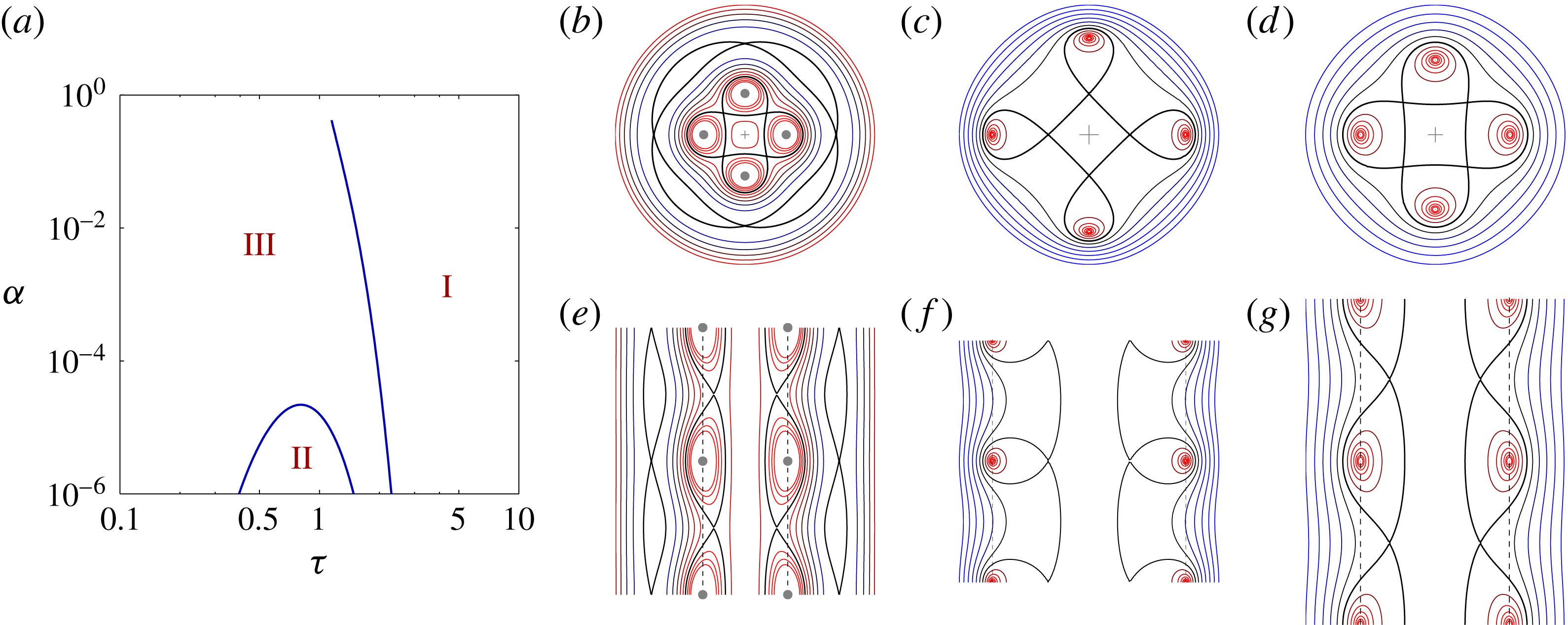
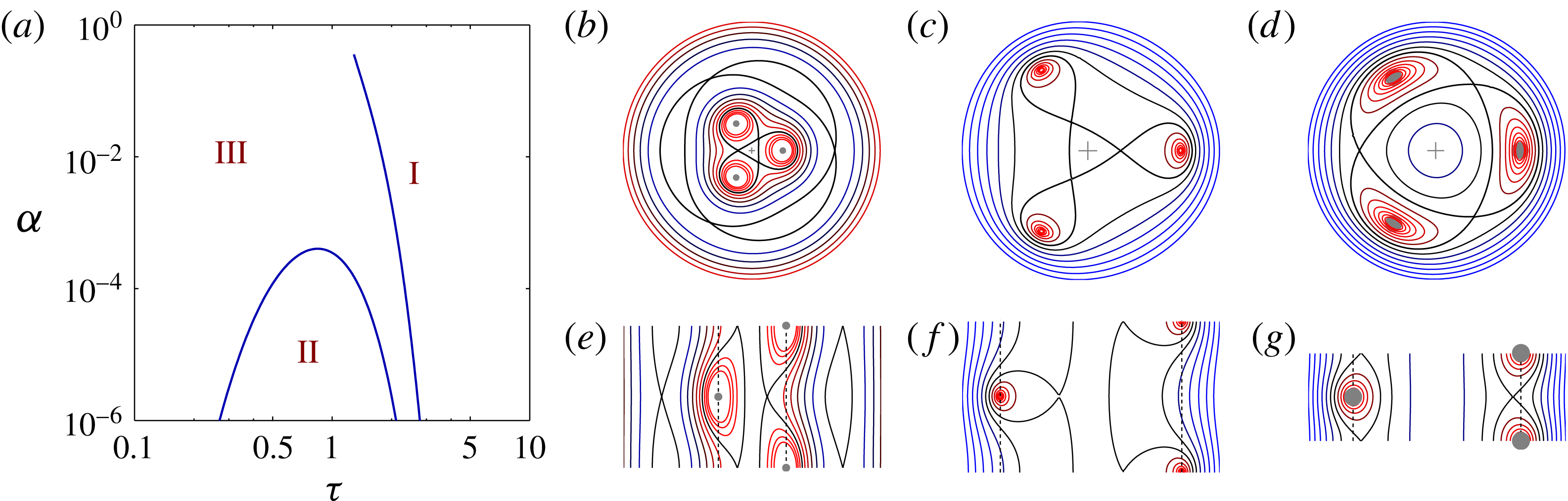
(a) Flow regimes for four helical vortices in the parameter plane
 $(\unicode[STIX]{x1D70F},\unicode[STIX]{x1D6FC})$
. (b–d) The helical stream function
 $\unicode[STIX]{x1D6F9}$
on the polar plane
 $(r,\unicode[STIX]{x1D703})$
for representative cases of each regime and (e–g) the corresponding stream function on the meridional plane
 $(r,z)$
(I–III from (b) to (d) and from (e) to (g)). (I) Large-pitch helices (example shown is
 $\unicode[STIX]{x1D70F}=2.0$
,
 $\unicode[STIX]{x1D6FC}=0.1$
), (II) thin small-pitch helices (example shown is
 $\unicode[STIX]{x1D70F}=0.8$
,
 $\unicode[STIX]{x1D6FC}=0.00001$
) and (III) thick small-pitch helices (example shown is
 $\unicode[STIX]{x1D70F}=1.4$
,
 $\unicode[STIX]{x1D6FC}=0.001$
).

The curves
 $\unicode[STIX]{x1D6F9}(r,\unicode[STIX]{x1D719})=C$
are streamlines of the helical flow
 $$\begin{eqnarray}u_{r}={\displaystyle \frac{1}{r}}{\displaystyle \frac{\unicode[STIX]{x2202}\unicode[STIX]{x1D6F9}}{\unicode[STIX]{x2202}\unicode[STIX]{x1D719}}},\quad u_{\unicode[STIX]{x1D719}}=-{\displaystyle \frac{\unicode[STIX]{x2202}\unicode[STIX]{x1D6F9}}{\unicode[STIX]{x2202}r}}.\end{eqnarray}$$
Because of the definition
 $\unicode[STIX]{x1D719}=\unicode[STIX]{x1D703}-z/l$
, the curves
 $\unicode[STIX]{x1D6F9}=C$
also represent the intersections with the polar plane
 $z=0$
of the stream surfaces of the three-dimensional flow
 $(u_{r},u_{\unicode[STIX]{x1D703}},u_{z})$
(see equations (8) and (9) of Hardin Reference Hardin1982). The intersections with any other polar plane
 $z=z_{0}$
have identical shapes but are rotated an angle
 $z_{0}/l$
. Similarly, the curves
 $\unicode[STIX]{x1D6F9}(r,-z/l)=C$
represent the intersections of the stream surfaces of the three-dimensional flow with the meridional plane
 $\unicode[STIX]{x1D703}=0$
; the intersections with any other meridional plane
 $\unicode[STIX]{x1D703}=\unicode[STIX]{x1D703}_{0}$
have identical shapes but are shifted a distance
 $l\unicode[STIX]{x1D703}_{0}$
along the
 $z$
axis.
The flow topology, or phase portrait in the language of dynamical systems, consists of the set of stagnation points plus the separatrices that divide the flow in regions of qualitatively different streamlines (or, in this steady case, particle trajectories). In the co-moving frame, the centrelines of the vortices, located at
 $(r,\unicode[STIX]{x1D703}_{i})=(a,2\unicode[STIX]{x03C0}\text{i}/N)$
, correspond to stagnation points of elliptic type. The symmetries of
 $\unicode[STIX]{x1D6F9}$
imply that other stagnation points, when they exist, are located following the same symmetries of the vortex array. We searched for these points with a numerical bisection method in order to perform a systematic exploration of the region of the parameter space defined by
 $10^{-6}<\unicode[STIX]{x1D6FC}<0.4$
and
 $0.1<\unicode[STIX]{x1D70F}<10$
for
 $N=1,2,3,4$
.
We found that for
 $N>2$
there are three different flow topologies that follow systematic patterns. Therefore, we describe them below in terms of an arbitrary
 $N>2$
, while figures 4 and 5 show two particular examples (
 $N=4$
and
 $N=3$
respectively).
The same as figure 4 but now for
 $N=3$
. (I) Large-pitch helices (
 $\unicode[STIX]{x1D70F}=2.0$
,
 $\unicode[STIX]{x1D6FC}=0.1$
), (II) thin small-pitch helices (
 $\unicode[STIX]{x1D70F}=0.8$
,
 $\unicode[STIX]{x1D6FC}=0.0001$
) and (III) thick small-pitch helices (
 $\unicode[STIX]{x1D70F}=0.5$
,
 $\unicode[STIX]{x1D6FC}=0.1$
).

Regime I: large-pitch vortices. This occurs for all values of
 $\unicode[STIX]{x1D6FC}$
when
 $\unicode[STIX]{x1D70F}$
is relatively large. The flow topology in the polar plane
 $r$
–
 $\unicode[STIX]{x1D703}$
has
 $2N+1$
elliptic points;
 $N$
correspond to the vortices and the rest have circulation opposite to the vortices: one is located on the axis and
 $N$
are located on a circle
 $r>R$
and are shifted with respect to the vortices by an angle
 $\unicode[STIX]{x03C0}/N$
. There are
 $2N$
hyperbolic points:
 $N$
are located on a circle
 $r>R$
along the same radial lines as the vortices while
 $N$
are located on a circle
 $r<R$
and are shifted with respect to the vortices by an angle
 $\unicode[STIX]{x03C0}/N$
. The flow topology in the meridional plane
 $r$
–
 $z$
indicates that there is a thin jet of fluid moving along the symmetry axis at a greater speed than the vortices.
Regime II: thin small-pitch vortices. This occurs when
 $\unicode[STIX]{x1D70F}$
and
 $\unicode[STIX]{x1D6FC}$
are relatively small. The flow topology in the polar plane
 $r$
–
 $\unicode[STIX]{x1D703}$
has
 $N+1$
elliptic points;
 $N$
correspond to the vortices while the additional point, located on the axis, has circulation of the same sign. There are
 $N$
hyperbolic points located on a circle
 $r<R$
along the same radial lines as the vortices. The flow topology in the meridional plane
 $r$
–
 $z$
indicates that the vortices trap only the fluid located in their immediate vicinity, leaving the rest behind.
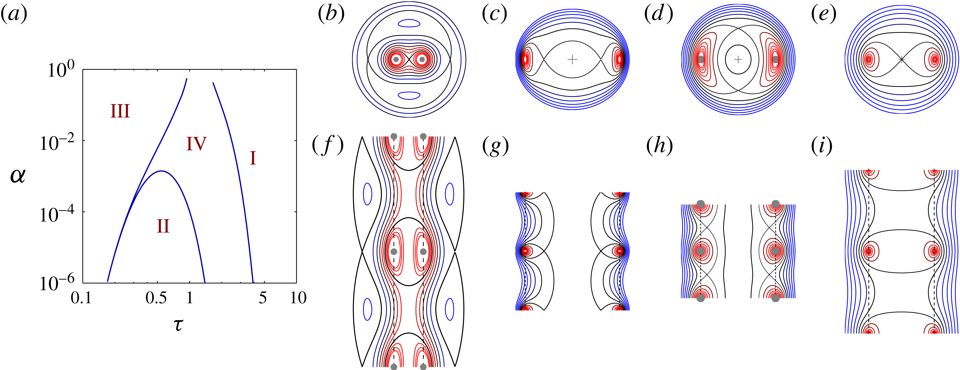
The same as figure 4 but now for
 $N=2$
. (I) Large-pitch helices (
 $\unicode[STIX]{x1D70F}=2.5$
,
 $\unicode[STIX]{x1D6FC}=0.2$
), (II) thin small-pitch helices (
 $\unicode[STIX]{x1D70F}=0.4$
,
 $\unicode[STIX]{x1D6FC}=0.0001$
), (III) thick small-pitch helices (
 $\unicode[STIX]{x1D70F}=0.4$
,
 $\unicode[STIX]{x1D6FC}=0.1$
) and (IV) medium-pitch helices (
 $\unicode[STIX]{x1D70F}=0.8$
,
 $\unicode[STIX]{x1D6FC}=0.01$
).

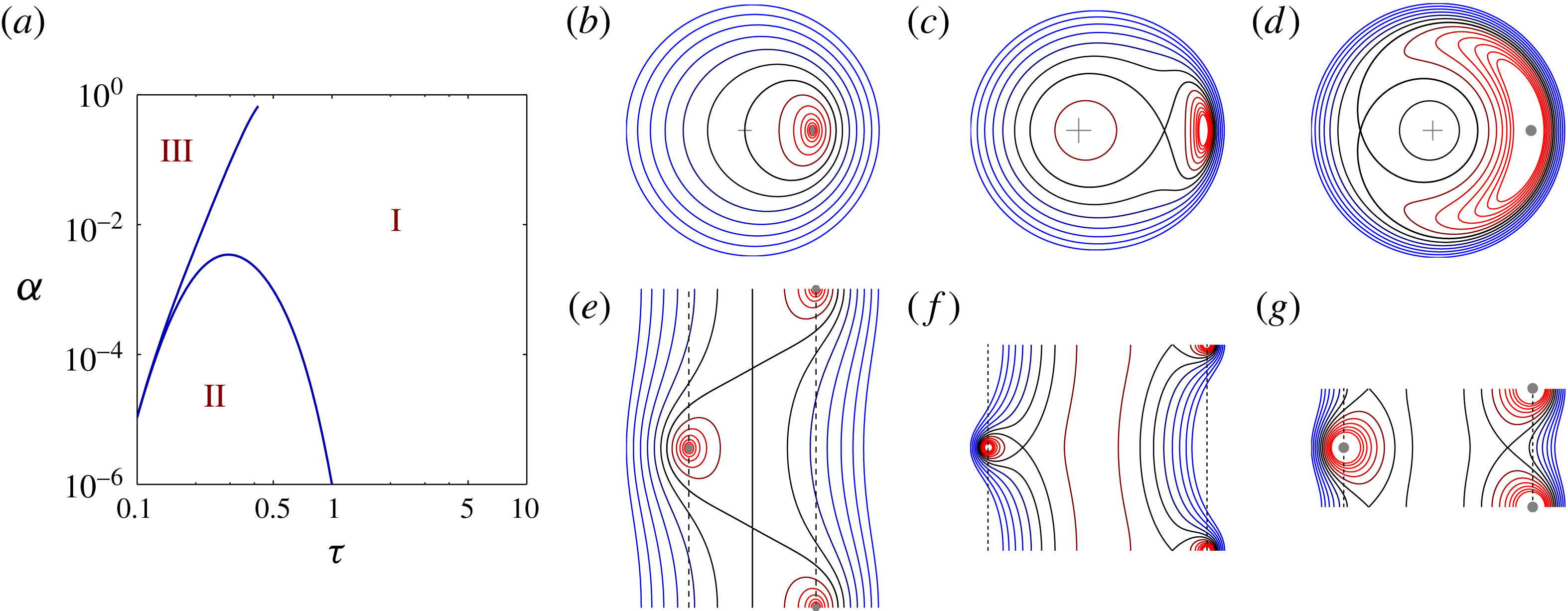
The same as figure 4 but now for
 $N=1$
. (I) Large-pitch helices (example shown is
 $\unicode[STIX]{x1D70F}=0.8$
,
 $\unicode[STIX]{x1D6FC}=0.05$
), (II) thin small-pitch helices (example shown is
 $\unicode[STIX]{x1D70F}=0.3$
,
 $\unicode[STIX]{x1D6FC}=0.0001$
) and (III) thick small-pitch helices (example shown is
 $\unicode[STIX]{x1D70F}=0.2$
,
 $\unicode[STIX]{x1D6FC}=0.05$
).

Regime III: thick small-pitch vortices. This occurs for relatively small values of
 $\unicode[STIX]{x1D70F}$
and relatively large values of
 $\unicode[STIX]{x1D6FC}$
. The flow topology in the polar plane
 $r$
–
 $\unicode[STIX]{x1D703}$
has
 $N+1$
elliptic points;
 $N$
correspond to the vortices while the additional point is located on the axis and has opposite circulation. The
 $N$
hyperbolic points are located on a circle of radius
 $r<R$
and are shifted with respect to the vortices by an angle
 $\unicode[STIX]{x03C0}/N$
. The flow topology in the meridional plane
 $r$
–
 $z$
indicates that there is a jet of fluid moving along the symmetry axis at a greater speed than the vortices. This is the type of flow that Fitzgerald (Reference Fitzgerald1899) speculated about.
Figure 6 shows the case
 $N=2$
. Its regimes II and III are as described for
 $N>2$
. Its regime I is similar to that described above but, in the polar plane
 $r$
–
 $\unicode[STIX]{x1D703}$
, it has only
 $2N$
stagnation points of elliptic type and only
 $2N-1$
points of hyperbolic type, and there is no jet along the axis. The extra flow regime (IV) occurs for vortices of intermediate pitch. The flow topology is similar to that of regime II but without the chain of fixed points for
 $r>R$
in the polar plane
 $r$
–
 $\unicode[STIX]{x1D703}$
.
Figure 7 shows the case
 $N=1$
. Its regimes II and III are as described for
 $N>2$
. Its regime I has, in the polar plane
 $r$
–
 $\unicode[STIX]{x1D703}$
, a single stagnation point, the vortex itself, and there is no jet along the axis.
The flow topology of a single helical vortex was first studied by Mezić et al. (Reference Mezić, Leonard and Wiggins1998) and Andersen & Brøns (Reference Andersen and Brøns2014). They, however, only took into account the binormal component of the vortex motion: Mezić et al. (Reference Mezić, Leonard and Wiggins1998) computed
 $U_{b}$
using both local and non-local effects whereas Andersen & Brøns (Reference Andersen and Brøns2014) used only local effects. As shown by Velasco Fuentes (Reference Velasco Fuentes2018), all calculations that do not include the tangential component give erroneous values of
 $U$
and
 $\unicode[STIX]{x1D6FA}$
, particularly for relatively small values of the vortex pitch: the ratio
 $U_{t}/U_{b}$
is approximately
 $0.3$
for
 $\unicode[STIX]{x1D70F}\approx 0.4$
when
 $\unicode[STIX]{x1D6FC}=0.1$
, whereas it is approximately
 $0.1$
for
 $\unicode[STIX]{x1D70F}\approx 0.2$
when
 $\unicode[STIX]{x1D6FC}=10^{-5}$
. Consequently, Mezić et al. (Reference Mezić, Leonard and Wiggins1998) and Andersen & Brøns (Reference Andersen and Brøns2014) found regime boundaries that were shifted with respect to the ones shown in figure 7.
5 Conclusions
We have combined the results of Okulov (Reference Okulov2004) and Velasco Fuentes (Reference Velasco Fuentes2018) to write down expressions for the velocities of a set of
 $N$
coaxial helical vortices that have, to leading order, uniform vorticity and circular cross-section. These expressions are valid for any number of vortices whose pitch (
 $\unicode[STIX]{x1D70F}$
) and radius (
 $\unicode[STIX]{x1D6FC}$
) satisfy
 $\unicode[STIX]{x1D6FC}^{2}\ll 1$
and
 $\unicode[STIX]{x1D70F}\geqslant 2N\unicode[STIX]{x1D6FC}/2$
.
For a given number of vortices, their pitch and radius determine their motion and capacity to transport fluid as follows: large-pitch vortices, whether thin or thick, translate slowly while carrying with them a large volume of fluid; thin small-pitch vortices translate fast but carry with them a small volume of fluid; thick small-pitch vortices translate at intermediate velocities, carry with them a moderate volume of fluid but, more significantly, push fluid forward along the axis of the vortices. The linear and angular velocities and the capacity to transport fluid increase considerably with the number of vortices.
Acknowledgements
I gratefully acknowledge A. Espinosa for performing the vortex-in-cell simulations used in figure 3, and two anonymous referees for their comments and criticisms on a previous version of this paper. This research was supported by CONACyT (México) under grant no. 169574.