





1. Introduction
1.1. Surficial meltwater routing on the Greenland ice sheet
Between 1992–2020, the Greenland ice sheet contributed 14 mm to global mean sea level rise, an average of 4.7 mm per decade (Otosaka and others, Reference Otosaka2023). This mass loss has primarily occurred through ice discharge (calving) and surface meltwater runoff (van den Broeke, Reference van den2016). Runoff produced in the ice sheet ablation zone flows downslope in supraglacial streams and rivers, with some 80% of the runoff at elevations >∼1000 m flowing directly to the bed via moulins (Smith and others, Reference Smith2015). The fate of the remaining 20% is less studied and includes supraglacial storage in wet snow and lakes or delivery to surface crevasses (Smith and others, Reference Smith2015). Study of moulins has outpaced that of crevasses in recent years (e.g. Smith and others, Reference Smith2017); it is not yet known whether crevasses deliver the melt to the bed or store it englacially to slowly refreeze (Poinar, Reference Poinar2015).
Surface crevasses are fractures that form from deviatoric stresses as ice flows over an irregular bed, through a constriction or responds to surge flow (Colgan and others, Reference Colgan2016; Zheng and others, Reference Zheng, Pritchard, Willis and Stearns2019; Reynolds and others, Reference Reynolds, Nowicki and Poinar2025). Meltwater can drive the deepening of crevasses through hydrofracture; if there is sufficient water volume, crevasses can fracture hundreds of meters or more down to the ice-sheet bed (Das and others, Reference Das2008; Krawczynski and others, Reference Krawczynski, Behn, Das and Joughin2009). These crevasses can then maintain a direct hydraulic connection for meltwater from the ice sheet surface to the ice sheet bed (Hooke, Reference Hooke1989). Consistent meltwater input through these fully-propagated crevasses can form moulins, which are near-vertical tunnel-like features that carry meltwater to the basal environment (Alley and others, Reference Alley, Dupont, Parizek and Anandakrishnan2005; Das and others, Reference Das2008).
Once in the basal environment, surface meltwater can affect the state of the subglacial drainage system (Bartholomew and others, Reference Bartholomew, Nienow, Mair, Hubbard, King and Sole2010; van de Wal and others, Reference van de Wal2015; Nienow and others, Reference Nienow, Sole, Slater and Cowton2017). During the early part of the melt season, surface meltwater inputs increase the water pressure in the subglacial system, increasing basal lubrication that speeds basal sliding velocities (Bartholomew and others, Reference Bartholomew, Nienow, Mair, Hubbard, King and Sole2010). Later in the melt season, sustained meltwater inputs can develop a channelized or efficient subglacial drainage system (Flowers, Reference Flowers2010). This decreases the overall water pressure and slows basal sliding velocities, allowing additional meltwater to enter the subglacial system without exceeding the hydraulic capacity of the channels or increasing sliding velocities (Schoof, Reference Schoof2010; Banwell and others, Reference Banwell, Hewitt, Willis and Arnold2016). Thus, surface meltwater input locations are important drivers of the spatial organization of subglacial channelization (Gulley and others, Reference Gulley, Grabiec, Martin, Jania, Catania and Glowacki2012; Mejia and others, Reference Mejia2022).
In order for a crevasse to deliver surface meltwater to the bed, conditions on the stress environment and meltwater supply must be met (e.g. Alley and others, Reference Alley, Dupont, Parizek and Anandakrishnan2005; Krawczynski and others, Reference Krawczynski, Behn, Das and Joughin2009; McGrath and others, Reference McGrath, Colgan, Steffen, Lauffenburger and Balog2011). These conditions vary regionally across the ice sheet, and investigations of various regions and techniques (field-based, model-based or both) have found different answers to this question. When crevasses lack meltwater input, crevasses typically propagate only tens of meters deep (Nye, Reference Nye1955). Field-informed studies from Pâkitsoq, central western Greenland, suggest that crevasses there transport supraglacial meltwater several hundred meters deep into the englacial system, where it can persist for decades before eventually refreezing and warming the surrounding ice by several degrees (Phillips and others, Reference Phillips, Rajaram, Colgan, Steffen and Abdalati2013; Lüthi and others, Reference Lüthi2015; Poinar and others, Reference Poinar, Joughin, Lenaerts and van den Broeke2016). On the other hand, McGrath and others (Reference McGrath, Colgan, Steffen, Lauffenburger and Balog2011) found that crevasse fields drain about 48% of the surface meltwater runoff to the bed, but the precise fraction may vary across different crevasses, crevasse fields, regions or across seasons. Similarly, Koziol and others (Reference Koziol, Arnold, Pope and Colgan2017) found that 47% of the surface meltwater runoff in Pâkitsoq is drained through crevasses. The body of observations suggests that crevasses serve as drainage pathways for meltwater to exit the supraglacial drainage system but whether they carry that water to the bed or retain it englacially is not generally known.
As surface velocity patterns vary over time, they will change the spatial distribution of crevasses (Koziol and Arnold, Reference Koziol and Arnold2018) and their role in delivering meltwater to the bed. Colgan and others (Reference Colgan2011) found a substantial expansion of crevassed area extent in Pâkitsoq between 1985–2009, while more recently, Chudley and others (Reference Chudley, Howat, King and MacKie2025) found the opposite: that crevassed area reduced between 2016–21 in central western Greenland. This suggests that there are substantial changes in the crevassing dynamics from decade to decade, but the year-to-year spatial evolution in the crevassed area of Pâkitsoq is not yet known.
Here we develop an automated method to detect crevasse fields from satellite imagery and apply it to Pâkitsoq, central western Greenland, over 2015–24, in order to measure the trend and interannual variability in the crevassed area extent. We also analyze the seasonal evolution of ice flow velocity across crevassed and moulin-drained areas to test the hypothesis that crevasses in Pâkitsoq carry meltwater to the bed, versus storing it englacially without delivering it to the bed. During the peak melt season, if meltwater reaches the bed through crevasses, its addition to the basal hydrologic system should locally reduce the effective pressure of the ice sheet, increasing ice flow speeds (Nienow and others, Reference Nienow, Sole, Slater and Cowton2017).
2. Background
2.1. Existing methods for crevasse detection
The study of crevasses on ice sheets has a long history. For many decades, field crews have performed crevasse detection on ice sheets for the safety of ground-based research teams (Cook, Reference Cook1956; Pings, Reference Pings1961; Taurisano and others, Reference Taurisano, Tronstad, Brandt and Kohler2006; Eder and others, Reference Eder, Reidler, Mayer and Leopold2008). Ground penetrating radar (GPR) is the most common on-site method. The radar waves can penetrate through the snow and ice layers to several tens to thousands of meters depth, depending on wavelength (Eder and others, Reference Eder, Reidler, Mayer and Leopold2008). Previous studies have collected and analyzed GPR data at study areas across a range of scales, including 1.8 km2 (Ravanel and others, Reference Ravanel, Lacroix, Le Meur, Batoux and Malet2022), 3 km2 (Kaluzienski and others, Reference Kaluzienski, Koons, Enderlin, Hamilton, Courville and Arcone2019) and 25 km2 (Walker and Ray, Reference Walker and Ray2019). Using GPR carried by helicopter, Thompson and others (Reference Thompson, Cook, Kulessa, Winberry, Fraser and Galton-Fenzi2020) surveyed a 296 km2 area. Assessing areas larger than this, however, requires a remote-sensing approach. Remote sensing allows features indicative of crevasses to be detected across wide areas, facilitating larger-scale hazard mapping (Colgan and others, Reference Colgan2011; Koike and others, Reference Koike, Yoshida, Omura, Shibuya and Doi2012; Chudley and others, Reference Chudley2021; Herzfeld and others, Reference Herzfeld, Trantow, Lawson, Hans and Medley2021; Marsh and others, Reference Marsh, Price, Courville and Floricioiu2021; Libert and others, Reference Libert, Wuite and Nagler2022). To date, these indicative features have included straight lines in visible imagery, bright places in radar imagery or trenches in DEMs (Colgan and others, Reference Colgan2011; Chudley and others, Reference Chudley2021; Marsh and others, Reference Marsh, Price, Courville and Floricioiu2021; Van Wyk de Vries and others, Reference Van Wyk de Vries, Lea and Ashmore2023; Chudley and others, Reference Chudley, Howat, King and MacKie2025) that have been detected manually by individual users, or algorithmically in an automated way. Manual analysis of remote sensing data (e.g. Colgan and others, Reference Colgan2011; Hoffman and others, Reference Hoffman2018) is a time-consuming endeavor.
Automated analyses of remote sensing imagery offer significant advantages. Recently, deep learning techniques have evolved, which enable data analysis over very large spatial scales, enabling a comprehensive dataset of crevasse distribution and ice sheet dynamics across the entire Antarctic ice sheet (Lai and others, Reference Lai2020; Zhao and others, Reference Zhao, Liang, Li, Duan and Liang2022; Surawy-Stepney and others, Reference Surawy-Stepney, Hogg, Cornford and Hogg2023). However, applying deep learning to detect crevasses from remote sensing imagery over the Greenland ice sheet has not yet been done. This is in part because of the difficulty of differentiating crevasses from other surface features, such as meltwater streams and lakes, which are prevalent in the Greenland ablation zone but rare across most of Antarctica. These distractor features are similar in scale (widths on the order of meters) to Greenland crevasses, which are substantially smaller and thus more difficult to resolve than Antarctic fractures (widths on the order of hundreds of meters). This work aims to address this challenge by developing an automated crevasse detection method for the Greenland ice sheet using remote sensing over a 629 km2 area of Pâkitsoq (Fig. 1a), a historically well-studied region in central western Greenland.
(a) Sentinel-2 RGB image from August 2019 median showing our 629 km2 study area of Pâkitsoq, central-western Greenland, within the red box, overlaid by 100 m surface elevation contours from BedMachine v5 (Morlighem and others, Reference Morlighem2017; Reference Morlighem2022). The green circle shows the crevasse field in panels (b) and (c). (b) WorldView-2 imagery acquired 8 June 2019 (2.2 km × 2.2 km) showing a crevasse field in green circle. Green dashed lines denote four specific crevasses visible in this crevasse field, labeled with their corresponding lengths. Blue arrows indicate supraglacial drainage features near this crevasse field. (c) Median of all Sentinel-1 SAR Level-1 Ground Range Detected HH single co-polarization scenes acquired in January 2020 (2.2 km × 2.2 km) showing the same crevasse field visible as a bright patch (green circle) with the four individual crevasses (green lines) discernible as thin linear features. Blue arrows again mark the two water features, which appear as bright nonlinear features.

Figure 1 Long description
Three-panel satellite map of Pâkitsoq, central-western Greenland. A) Sentinel-2 map from August 2019 shows a 629 km study area outlined in a red box, with 100 m elevation contours. North is at the top. B) WorldView-2 map from June 2019 highlights a crevasse field within a green circle, with four labeled crevasses and blue arrows indicating supraglacial drainage flow. C) Sentinel-1 SAR map from January 2020 shows the same crevasse field as a bright patch, with crevasses as thin lines and blue arrows marking water features. The maps illustrate the crevasse field′s visibility in both optical and SAR imagery, emphasizing drainage features. The red box indicates the broader study area, the green circle marks the specific crevasse field and contours represent elevation lines. Scale bars show 1 km extent.
2.2. Crevasse detection using Sentinel-1 SAR imagery
The Sentinel-1 satellite constellation carries Synthetic Aperture Radar (SAR) instruments that transmit C-band microwaves at 5.3 GHz frequency toward a surface, then receive back the reflected microwave signal (Torres and others, Reference Torres2012). In areas where the ice surface is smooth, SAR microwaves reflect a small portion of the microwave energy back to the receiver, making the surface appear dark in the produced image. Where the surface is rough, backscatter is higher, making the terrain appear brighter. SAR data thus provides a clear contrast between crevasse fields and non-crevassed ice, as rough crevasse fields appear bright and smooth ice surfaces appear dark in SAR imagery. The spatial resolution of Sentinel-1 SAR imagery is 10 m, which is larger than the typical width of an individual crevasse (∼2 m). A pixel that overlaps a crevasse should therefore appear somewhat brighter than its surroundings, although not as bright as if a crevasse occupied the entirety of the pixel. However, due to the long length of most crevasses (at least a few hundred meters, shown in Fig. 1b and c), a single crevasse appears in Sentinel-1 SAR as a continuous line of brighter-than-average pixels. Furthermore, crevasses often cluster together in crevasse fields, which appear as bright patches with a distinct linear pattern (Fig. 1c).
Alternative remote-sensing data sources that resolve crevasses include optical image data from the European Space Agency’s Sentinel-2 satellite constellation (10 m multispectral spatial resolution), commercial WorldView-1 and WorldView-2 satellites (0.5 m panchromatic and 2 m multispectral spatial resolution, respectively) and NASA/USGS’s Landsat-8/9 satellite constellation (15 m panchromatic and 30 m multispectral spatial resolution). In all of these sources, even in the highest-resolution WorldView-1 data, some crevasses and crevasse fields are not visible due to snow cover, cloud cover or daylight conditions. These problems are not faced by Sentinel-1, whose C-band SAR can penetrate the dry snowpack to a maximum depth of ∼9 m, and typically a few meters in our study area (Rignot and others, Reference Rignot, Echelmeyer and Krabill2001). This makes Sentinel-1 imagery a very suitable dataset for detecting crevasses. One limitation, however, of polar-orbiting satellites is that these may miss crevasse fields that are oriented unfavorably to look direction (Hoffman and others, Reference Hoffman2025). For instance, some features may be visible only in ascending orbits, others only in descending orbits and other features not in either (Hoffman and others, Reference Hoffman2025).
Crevasses at a perpendicular direction to the SAR incidence angle scatter back higher energy off the crevasse edge or wall facing the sensor, producing a bright surface return (Fig. 2). On the other hand, crevasses encountered at a parallel direction do not face the backscatter-enhancing wall and thus undergo higher forward scattering, producing a darker surface return (Marsh and others, Reference Marsh, Price, Courville and Floricioiu2021).
Sentinel-1 SAR polarization on crevasse surface: (a) HH single co-polarization mode transmits and receives horizontally polarized microwaves. The HH mode is sensitive to surface slope, so crevasses create high backscatter and low forward scatter, producing a bright return in crevassed areas. (b) VV single co-polarization mode transmits and receives vertically polarized microwaves. The VV mode is sensitive to surface roughness, so crevasses cause low backscatter and high forward scatter. This creates dark returns in crevassed areas. (c and d) HV and VH cross-polarization modes combine some of the features of the co-polarization (HH and VV) modes, sometimes producing bright returns in crevassed areas but generally returning lower energy overall. The cross-polarization modes produce contrast between crevassed and non-crevassed areas but suffer from higher energy loss.
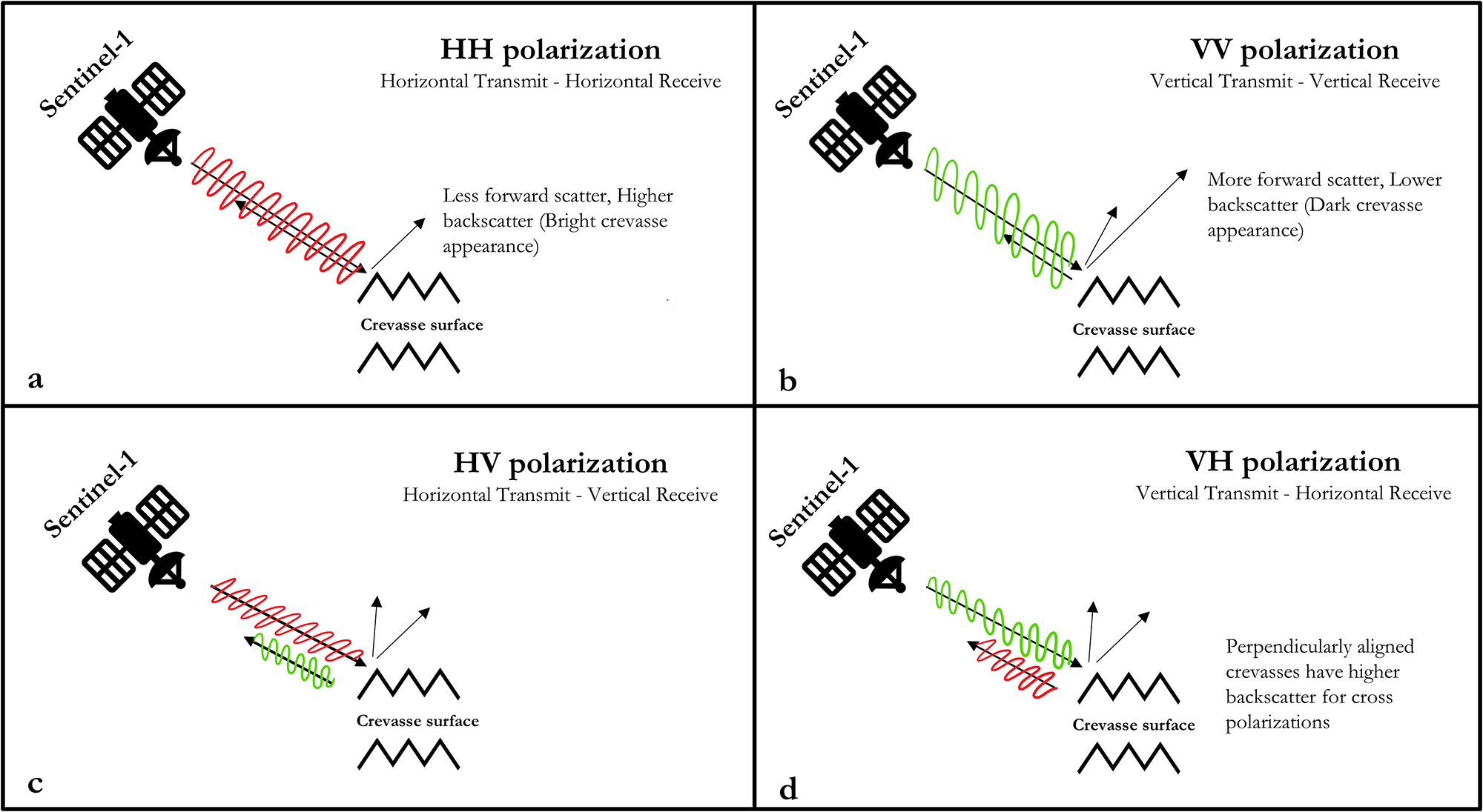
Figure 2 Long description
Four diagrams illustrate Sentinel-1 SAR polarization modes on crevasse surfaces. The first diagram, labeled ′a′, shows HH polarization with horizontal transmit and receive. It indicates less forward scatter and higher backscatter, resulting in a bright crevasse appearance. The second diagram, labeled ′b′, depicts VV polarization with vertical transmit and receive, showing more forward scatter and lower backscatter, leading to a dark crevasse appearance. The third diagram, labeled ′c′, presents HV polarization with horizontal transmit and vertical receive, highlighting the crevasse surface. The fourth diagram, labeled ′d′, illustrates VH polarization with vertical transmit and horizontal receive, noting that perpendicularly aligned crevasses have higher backscatter for cross polarization.
Study area, a 30.72 km × 20.48 km area of Pâkitsoq, shown in Figure 1a. We divide this area into regions A–F. Region A shows 15 m ice sheet margin black outlines from GIMP ice mask (Howat and others, Reference Howat, Negrete and Smith2014; Reference Howat2017). We use the median of all Sentinel-1 SAR Level-1 GRD HH single co-polarization scenes acquired in January 2020 for training the model. Manually digitized ground-truth labels containing crevasse field (green polygons) and remnant stream/lake (blue polygons) are used as training (purple boxes) and validation (cyan box) datasets.

Figure 3 Long description
Six regions labeled A to F in the Pâkitsoq area are shown with overlays indicating crevasse fields, streams/lakes, training and validation datasets. Region A displays crevasse fields outlined in green and streams/lakes in blue, with training areas marked in purple. Region B shows similar features with crevasse fields and streams/lakes, also marked for training. Region C highlights crevasse fields and streams/lakes, with training areas. Region D continues the pattern with crevasse fields and streams/lakes, marked for training. Region E is designated for validation, showing a mix of crevasse fields and streams/lakes. Region F includes crevasse fields and streams/lakes, marked for training. Each region is bordered in purple and a scale bar indicates 5 km for reference.
Sentinel-1 SAR has four polarization modes: Horizontal Transmit and Horizontal Receive (HH) and Vertical Transmit and Vertical Receive (VV) single co-polarization, Horizontal Transmit and Vertical Receive (HV) and Vertical Transmit and Horizontal Receive (VH) dual-band cross-polarization. Figure 2 illustrates the differences in backscatter among these modes. HH single co-polarization mode transmits and receives microwaves in the horizontal direction; when the transmit/receive orientation is perpendicular to the crevasse strike, the crevasse walls reflect back high scatter and consequently produce low forward-scatter. VV single co-polarization mode transmits and receives microwaves in the vertical direction. The vertically polarized waves are sensitive to surface roughness in any direction, so crevassed surfaces, regardless of their strike, produce high forward-scatter, in contrast to smooth surfaces that reflect higher scatter. This makes crevasses appear dark and smooth surfaces appear bright in VV polarization. Finally, HV and VH dual-band cross-polarization modes each use both the horizontal and vertical directions. The vertical portion of HV and VH polarization produces forward-scattering or double-bounce backscattering on crevasses, which makes them appear dark, while smooth surfaces appear bright. Both HV and VH polarization modes yield high contrast between crevassed and non-crevassed areas (Marsh and others, Reference Marsh, Price, Courville and Floricioiu2021). However, the cross-polarization modes produce lower backscatter overall compared to the like-polarization modes, making dimmer images that have an overall less separable signal between crevassed and smooth areas. Therefore, we judge the HH single co-polarization SAR mode to work best for crevasse field detection in our application because it tends to generate bright observations with good contrast between crevasse fields and uncrevassed ice, and because it reduces noise when a double-bounce backscattering occurs.
SAR backscatter from the Sentinel-1 satellite is sensitive to the presence of water in ice and snow. Thus, during the melt season when the surface is wet, water will absorb some microwave radiation, making the ice-sheet surface appear darker in the SAR imagery than at other times of year (Marin and others, Reference Marin2020). This makes crevasse detection using SAR imagery more difficult, as there are lower returns from all surfaces, including crevassed areas. Therefore, we judge that January–April, when the surface is dry and therefore has low absorption of microwave radiation, are optimal for detecting crevasse fields.
2.3. Crevasse detection using deep learning
Deep learning models comprise multiple layers of neural networks that extract information from input data. We use a semantic segmentation-based convolutional neural network (CNN), which detects features from input images using supervised classification (LeCun and others, Reference LeCun, Bengio and Hinton2015). Supervised classification requires that each input image be labeled or classified; the CNN ingests the labels to learn patterns inherent in the target features (Long and others, Reference Long, Shelhamer and Darrell2015). CNNs comprise interconnected nodes that are arranged in layers. Each node takes inputs, processes them and produces an output that it sends to the next layer of nodes (Buduma and others, Reference Buduma, Buduma and Papa2022). The CNN assigns weights to the connections between the nodes, then modifies these weights during the training process to enhance the performance of the network against the known labels (Alzubaidi and others, Reference Alzubaidi2021). Most image-processing CNNs are equipped with multiple convolution filters by which the models detect the target class from all features obtained through convolution (Gu and others, Reference Gu2018). These convolution filters are small matrices that convolve across the image to find natural edges, lineations or feature boundaries in the image (Zeiler and Fergus, Reference Zeiler and Fergus2014).
Recent studies have harnessed the potential of CNN-based deep learning to identify fractures on ice sheets in Antarctica (Lai and others, Reference Lai2020; Zhao and others, Reference Zhao, Liang, Li, Duan and Liang2022; Surawy-Stepney and others, Reference Surawy-Stepney, Hogg, Cornford and Hogg2023). However, no study has yet used CNNs for the identification of Greenland crevasses. The closest study is Chudley and others (Reference Chudley2021), who applied a random forest classifier to elevation data over a small (7 km2) field study area in western Greenland. Random forest classifiers excel at classifying features of pre-identified types, for example healed crevasses, narrow crevasses and wide or water-filled crevasses (Chudley and others, Reference Chudley2021); however, they are less able to broaden the detections into, for instance, a general ‘crevasse’ type. For this capability, CNNs are optimal.
We use a CNN-based deep learning algorithm to extract patterns from Sentinel-1 SAR satellite imagery to detect crevasses at a regional scale. We use a modified version of the U-Net deep learning architecture with fully connected convolutional filters (Ronneberger and others, Reference Ronneberger, Fischer and Brox2015). U-Net improves upon the base CNN algorithm by upsampling the extracted features to the same (or similar) pixel resolution and orientation as the original input image. Thus, the U-Net model not only detects target features in an image but also identifies their spatial locations. U-Net is designed to locate specific user-defined classes within an image by analyzing the image at multiple scales. U-Net has been previously used for detecting glacier calving fronts in Greenland (Baumhoer and others, Reference Baumhoer, Dietz, Kneisel and Kuenzer2019; Mohajerani and others, Reference Mohajerani, Wood, Velicogna and Rignot2019; Cheng and others, Reference Cheng2021). It has also been implemented for detecting fractures on Antarctic ice shelves (Lai and others, Reference Lai2020; Zhao and others, Reference Zhao, Liang, Li, Duan and Liang2022; Surawy-Stepney and others, Reference Surawy-Stepney, Hogg, Cornford and Hogg2023). For example, Surawy-Stepney and others (Reference Surawy-Stepney, Hogg, Cornford and Hogg2023) used a shallow-layered U-Net to detect large (∼200 m width) fractures on ice shelves and smaller (∼50 m width) fractures on grounded ice; the latter is similar to a small crevasse field in Greenland. Their results suggest that small crevasses are significantly more difficult to identify than large crevasses. We address this challenge by developing a new model based on U-Net to detect densely spaced, narrow crevasses on the Greenland ice sheet.
3. Methods
3.1. Study area and remote sensing data
Our study area encompasses a ∼30 × 20 km2 area of the Pâkitsoq region in central western Greenland, centered at 69.47°N, 49.72°W. This region has a long history of glaciological studies (Thomsen and others, Reference Thomsen, Olesen, Braithwaite and Weidick1989; Colgan and others, Reference Colgan2011; Andrews and others, Reference Andrews2014; Lüthi and others, Reference Lüthi2015; Koziol and others, Reference Koziol, Arnold, Pope and Colgan2017; Mejia and others, Reference Mejia2022). Particularly, Hoffman and others (Reference Hoffman2018) used WorldView-2 satellite imagery to manually digitize the locations of crevasse fields in a subset of our study area over 2009–11, making a valuable independent comparison dataset.
Figure 4 shows the complete crevasse detection workflow using remote sensing and deep learning. We constructed and analyzed a representative wintertime median scene from Sentinel-1 SAR Level-1 Ground Range Detected (GRD) imagery covering 30.72 km × 20.48 km in Pâkitsoq. We constructed this scene from five individual Sentinel-1 scenes, acquired on January 1, 7, 13, 19 and 25 of 2020, which we accessed using Google Earth Engine (Gorelick and others, Reference Gorelick, Hancher, Dixon, Ilyushchenko, Thau and Moore2017). Google Earth Engine pre-processes Sentinel-1 SAR raw scenes using the Sentinel-1 Toolbox, which applies thermal noise removal, radiometric calibration to convert the radar backscatter coefficient to decibels using log-scaling for normalization, and terrain correction to orthorectify the scenes (Veci and others, Reference Veci, Lu, Foumelis and Engdahl2017). We selected the HH single co-polarization, interferometric swath mode and ascending orbit, generated their pixel-by-pixel median over the five acquisition dates, and exported the resultant median scene as a 64 bit GeoTiff raster with the native 10 m spatial resolution. Because of relatively slow ice speeds in our study area (∼100 m yr−1), this temporal median method introduces only a low amount of feature blurring. Across the 25 days of January, the ice moved ∼8 m, or 1 pixel. Across 4 months of spring (January–April), the movement is ∼33 m, or 3 pixels. This keeps the crevasse fields, which are hundreds to thousands of meters wide, intact, while producing some blurry effects by tens of meters around the edges of the crevasse fields. This was the best way we tested that could reduce speckle noise enough to make the deep learning model perform well (Supplementary Section S1).
Automated crevasse detection workflow. From the top down: Data collection in Google Earth Engine: export Sentinel-1 SAR imagery for Pâkitsoq region with outlined parameters → Pre-processing in QGIS: change format of the exported rasters + ground-truth labels → MimiNet workflow: input processed images and labels to train model + perform model hyperparameter tuning = Crevasse detection + metric scores → Post-processing: merge and vectorize all crevasse field detections → Final output of map of crevasse fields.

Figure 4 Long description
Automated crevasse detection workflow: Step 1, data collection in Google Earth Engine with Sentinel-1 SAR imagery for the Pâkitsoq region. Step 2, pre-processing in QGIS involves input rasters from six sub-regions, creating a vector grid and manual digitization for labeling. Step 3, U-Net compatibility steps include resizing and format conversion. Step 4, MimiNet workflow with model training using input rasters and labels, split into 85 percent training and 15 percent validation. Decision points include model hyperparameter tuning and accuracy assessment. Step 5, post-processing merges and vectorizes crevasse detections. Final output is a map of crevasse fields. The flowchart uses process boxes and a diamond shape for the final output.
We divided our study area into six regions, each 10.24 km × 10.24 km (Fig. 3), and allocated them as training and testing (regions A, B, C, D and F) and validation (region E) datasets. We next subdivided each region raster into four tiles (5.12 km × 5.12 km each) to reduce computational runtime and maintain compatibility with U-Net, which expects 512 × 512 pixel inputs. Thus, six regions divided into four tiles yielded 24 tiles each of 512 × 512 pixels; we used 20 tiles as the training and testing data and 4 tiles as the validation data. We chose region E to be the validation dataset as it has a mix of crevasse fields, supraglacial streams and lakes. The validation dataset consisted of Sentinel-1 median scenes of January 2018, 2019 and 2020 (Supplementary Table S2) to increase the variability in surface conditions
3.2. MimiNet crevasse field detection
We developed MimiNet, a deep learning workflow that adapts U-Net to the specific problem of crevasse field detection on the Greenland ice sheet ablation area from Sentinel-1 SAR images. Like U-Net, MimiNet uses image segmentation, which is a pixel-based classification method that requires ground-truth labels that identify target features in the training dataset. The primary target feature of MimiNet is crevasse fields, but these features are interspersed with the remnants of summertime meltwater features, such as supraglacial streams and supraglacial lake beds, which often appear similarly bright in Sentinel-1 SAR imagery (Surdu and others, Reference Surdu, Duguay, Brown and Fernández Prieto2014). To avoid conflating crevasse fields with these remnant meltwater features, we trained the model to identify three classes: non-features (ice without crevasses or streams), crevasse fields and remnant supraglacial streams/lakes. We manually created labels by outlining all features in the median of all Sentinel-1 scenes acquired over January 2020 across our study area (Section 3.1), using a map scale of 1:20000 and a digitization radius of 150–600 m (15–60 pixels in Sentinel-1 imagery) in QGIS. Labels for Region E in January 2018 and 2019 median scenes were generated by a different individual to strengthen the model training process. Figure 5 shows the processing chain: the input raster, the manually annotated vector shapefile and finally the three categories of rasterized labels. Our three target classes are as follows: non-features (white regions), crevasse fields (green regions) and remnant stream/lake (blue regions).
(From left to right) The median of all Sentinel-1 SAR Level-1 GRD HH single co-polarization scenes acquired in January 2020 over the training region F (1024 px × 1024 px) ⇒ Manually classified vector shapefile containing crevasse fields (green polygons) and remnant stream/lake (blue polygons) ⇒ Rasterized labels containing three classes: non-features (class 0, white region), crevasse fields (class 1, green regions) and remnant stream/lake (class 2, blue regions).

Figure 5 Long description
Three-panel workflow figure illustrating a process from satellite imagery to labeled maps. The left panel shows a grayscale satellite image labeled ′Training Region F′ with a scale bar of 800 meters and a north arrow. The middle panel displays manually digitized outlines with green polygons for crevasse fields and blue for streams or lakes, labeled ′Manually Digitized Shapefile.′ The right panel presents rasterized labels with green for crevasse fields, blue for streams/lakes and white for non-features, labeled ′Rasterized Label.′ Arrows indicate the transformation from one panel to the next.
3.2.1. MimiNet model structure
We adapted the U-shaped U-Net Architecture to develop MimiNet, as shown in (Fig. 6). The left portion of Figure 6 shows the downsampling path and the right portion shows the upsampling path. MimiNet extracts features through three layers in the downsampling path. The inputs are 512 × 512 pixel single-band 8 bit images with pixel values from 0–255. To gain compatibility with U-Net, we converted both the raster (Fig. 3) and ground-truth labels (Fig. 5) to 8 bit images using the LZW Lossless Image Compression method in QGIS. In each layer, the image is processed through two 3 × 3 convolution filters and then one 2 × 2 max pooling filter. Each convolution filter (yellow arrow) convolves across the image to extract feature maps. In the first layer, the two convolution operations produce 16 extracted feature maps per image. In the second layer, the two convolution operators extract 32 feature maps, and 64 feature maps in the third layer. At the end of each layer along the downsampling path, a max pooling operator (pink arrow) takes the maximum pixel values across 2 × 2 windows, thereby reducing the spatial size by a factor of four (a factor of two in each direction), i.e. from 512 × 512 to 256 × 256 in the second layer, and from 256 × 256 to 128 × 128 in the third layer. Next, the 64 feature maps extracted at the third layer are upsampled to regain the spatial size lost along the downsampling path. A 2 × 2 upsampling filter (purple arrow) duplicates rows and columns of the image matrix, then the feature maps are cropped and concatenated with the feature maps from each downsampling layer. Two more 3 × 3 convolution filters are applied after every upsampling, and then a final 1 × 1 convolution filter (also known as the activation function) is applied to reduce the image depth from 16 feature maps to the number of target classes (three), producing a 512 × 512 × 3 output image.
MimiNet model structure for detecting crevasses on the Greenland ice sheet. The downsampling and upsampling design from its U-shaped architecture. Different arrows indicate the filters used in the model. The raster input is 512 pixels × 512 pixels from the median of all Sentinel-1 SAR Level-1 GRD HH single co-polarization scenes acquired in January 2020 (top-left) and the model output (top-right) contains detected crevasse fields (gray regions), remnant supraglacial streams/lakes (white regions) and non-feature class (black regions).

Figure 6 Long description
The MimiNet model structure for detecting crevasses is illustrated, featuring a U-shaped architecture with downsampling and upsampling paths. On the top left, the raster input is shown as a 512 by 512 by 1 image. This input is processed through the downsampling path, which includes three layers. In Layer I, the input is transformed into a 512 by 512 by 16 image using two 3 by 3 convolution filters, indicated by yellow arrows, followed by a 2 by 2 max pooling filter, shown with a pink arrow, reducing the size to 256 by 256 by 16. Layer II further processes the image to 256 by 256 by 32 using similar filters and then to 128 by 128 by 32. In Layer III, the image is reduced to 128 by 128 by 64. The upsampling path begins with a 2 by 2 upsampling filter, represented by a purple arrow, which increases the size back to 256 by 256 by 64. The feature maps are then copied and concatenated with those from the downsampling layers, as indicated by a black arrow. Additional 3 by 3 convolution filters are applied, followed by a 1 by 1 activation function, shown with a red arrow, to produce the final output of 512 by 512 by 3. The model output, displayed on the top right, shows detected crevasse fields, remnant supraglacial streams or lakes and non-feature classes.
3.2.2. Ghub workflow implementation
We developed and ran MimiNet on Ghub, a gateway for datasets, analysis tools and supercomputing resources for ice sheet science (Sperhac and others, Reference Sperhac2021). We used the Ghub JupyterLab tool (Clark, Reference Clark2023) for its functionality of opening terminal, console and Python editing modules, as well as using multiple notebooks on one browser tab. We authenticated a GitHub repository to contain all files required for this project for managing version control during project development. We used Keras, an open-source deep learning library built with the TensorFlow machine learning framework (Abadi and others, Reference Abadi2016) and TensorFlow 2.15 (TensorFlow Developers, 2023) for our MimiNet model. We modified the TensorFlow Version 2-based implementation of U-Net (Akeret and others, Reference Akeret, Chang, Lucchi and Refregier2017) to ensure compatibility with our workflow.
3.2.3. Model training workflow
Supervised learning guidelines stipulate using ∼85% of a labeled dataset to train the model and the remaining ∼15% to validate the trained versions of the models (Moolayil and Moolayil, Reference Moolayil and Moolayil2019). As our model requires a TensorFlow Dataset structure input, we utilized the TensorFlow data API to build our model input pipeline. This creates an efficient dataset pipeline that saves computation time regardless of dataset size and increases pre-processing options. We built MimiNet around the U-Net model structure, which requires definition of the expected input image size and number of channels, the number of target classes, the number of model layers, the number of feature maps in the first layer, the size of the convolution and max-pooling filters, the dropout rate, the type of padding used during image convolutions and the type of activation function used for the final output.
We explored optimization of key parameters to achieve the best model performance output. We manually varied the model parameters and experimented in an ad hoc way through reasonable parameter limits. We evaluated the performance of each model by assessing the accuracy, loss and Intersection over Union (IoU) score for both training and validation datasets (Supplementary Table S1). These evaluation metrics are the functional form of the calculation of loss (inaccuracy) between the labels and predictions. We varied the optimizer, dropout rate, initializer and regularizer to prevent model underfitting or overfitting. The optimizer function is used to converge the model quickly while preventing underfitting using the learning rate hyperparameter, which controls how fast the model adjusts its coefficients across subsequent iterations. We varied the learning rate from 0.0001–0.1, depending on the type of the optimizer. We assigned a rate to the dropout layer to randomly drop input units as the model adjusts weights between the nodes, which also helps prevent model overfitting. We tested dropout rates of 0–0.5. The kernel initializer and regularizer work together as the model adjusts weights during training for each layer. The initializer sets how to initialize weights, whereas the regularizer adds a penalty in cases where the model over-adjusts weights. We tested initializers known as Wendy, Ryan and Bratwurst and varied the regularizer over 0.1–100.
We began model training by defining the training and validation datasets, the number of epochs, batch size and all necessary callback functions. Each epoch refers to a complete pass of the whole dataset through the model; between epochs, model weightings are adjusted to produce a new version of the model. The batch size refers to the number of training files in a model forward and backward pass or the number of training files to be processed in a model run. We trained our model for 900 epochs with a batch size of one. We also used callback functions to track and monitor model training for every step, which can be utilized to stop model training as the model metrics stop improving. We used TensorBoard, a model parameter organization and visualization tool incorporated in TensorFlow Version 2, to visualize the model training progress at each iteration to define callback functions. TensorBoard displays the training performance at every step, shows what the model learned from the training samples, and plots the evaluation metrics.
3.2.4. Model evaluation
We evaluated our model outputs using accuracy, loss and IoU across the training and validation datasets. Accuracy refers to the fraction of correct predictions (true positives [TPs] and true negatives), while loss refers to the fraction of wrong predictions (false positives [FPs] and false negatives [FN]). We measured accuracy using the Sparse Categorical Accuracy function to suit our three discrete, non-overlapping classes (Moolayil and Moolayil, Reference Moolayil and Moolayil2019). We measured the training loss similarly, using the Sparse Categorical Cross Entropy function (Terven and others, Reference Terven, Cordova-Esparza, Ramirez-Pedraza, Chavez-Urbiola and Romero-Gonzalez2024).
We used the IoU metric to evaluate the overall model performance. This is the most widely used evaluation metric for semantic image segmentation problems (Cheng and others, Reference Cheng2021; Zhang and others, Reference Zhang, Liu, Huang and Ng2021; Chu and others, Reference Chu, Yao, Duan, Chen, Li and Pang2022; Herrmann and others, Reference Herrmann2023; Loebel and others, Reference Loebel2023). This metric is defined as follows:
 \begin{equation}IoU\, = \,\frac{{TP}}{{TP\, + \,FP\, + \,FN}}\end{equation}
Here, TP is the number of correctly predicted pixels that belong to a given class, FP is the number of incorrectly predicted pixels for that class, and FN refers to the number of missed predictions for that class. Possible values of IoU range from 0–1, where 1 means the model achieved 100% correct detection and 0% errors. We used the Jaccard similarity coefficient score metric from the scikit-learn open-source machine-learning library (Pedregosa and others, Reference Pedregosa2011) to calculate the IoU scores for each class in our model predictions, as well as the mean IoU score across all three classes for evaluating the overall model performance.
The IoU provides a balanced metric by excluding the true negatives. For our application, this is advantageous because of the imbalanced classes: most of our pixels are in class 0 (non-features), whereas our scientific interest is in class 1 (crevasse fields). Thus, a poor-quality model could nevertheless achieve good accuracy by over-predicting class 0, equivalent to performing well at identifying featureless ice surfaces at the expense of identifying crevasse fields. We prevent this possibility by excluding true negatives in our evaluation metric (Eqn 1), instead emphasizing TPs (correctly identified crevasse fields).
3.3. Analysis of crevasse extent in Pâkitsoq over 2015–24
We studied the changes in the total crevassed area in our study region by applying our automated crevasse detection workflow to summary images we generated from the Sentinel-1 HH single co-polarization images over 2015–24. Specifically, we constructed pixel-by-pixel annual median images for all available imagery each spring using Google Earth Engine (see Section 3.1), which we defined as January through April of each year in the 10 year period. This was because in all years except for 2020, we found that January medians of HH polarization contained a large amount of speckle noise, which interferes with accurate crevasse field detection. We performed manual inspection of the February, March and April scenes; we found no substantial difference in surface characteristics. This is likely due to relatively uniform conditions across the winter season in western Greenland; melt in this region typically begins in May (Wang and others, Reference Wang, Sharp, Rivard and Steffen2007; Andrews and others, Reference Andrews2014; Mejia and others, Reference Mejia2021). Therefore, we expanded the time range over which we took the median to maximize speckle removal while still remaining within the winter season for minimal meltwater presence. The ice flow in our study area of Pâkitsoq typically moves ∼50–100 m within the 4 month time period that the median scenes span. This makes us lose the ability to detect individual crevasses while retaining the capability of distinguishing crevasse fields with blurry edges of a few pixels. We used manually digitized crevasse field shapefiles from Hoffman and others (Reference Hoffman2018), which cover 3 years (2009, 2010 and 2011), to extend the study of the total crevassed area in Pâkitsoq farther back in time.
3.4. Uncertainty in crevassed area
We used the six models whose hyperparameter combinations are shown in Supplementary Table S1 to calculate the uncertainty of the crevassed area in Pâkitsoq over our study area. To do this, we trained all six models on Sentinel-1 HH single co-polarization of the January 2020 median imagery, but we varied the label datasets across these models. We trained five models on labels of crevasse fields digitized on this same Sentinel-1 image (Models 6, 7, 9, 16 and 17; Supplementary Table S1). We trained the three models (also Models 6, 7 and 9) on labels digitized based on WorldView-1 imagery acquired on 6 July 2010 and WorldView-2 imagery acquired on 4 August 2013. Different users generated the two label datasets, but each user followed the same rules (described in Section 3.2). We used these eight trained models to calculate the standard error of the mean of the total and sub-regional crevassed area for every year in our 10 year study period, following:
 \begin{equation}SE\, = \,\frac{{{\sigma _{YM\,}}}}{{\sqrt {{N_M} - \,1} }}\end{equation}
where σYM refers to the yearly standard deviation of our eight models (Models 6, 7, 9, 16 and 17 trained on Sentinel-1-based labels and Models 6, 7 and 9 trained on WorldView-1- and WorldView-2-based labels) and NM = 8, the number of models. The quantity NM − 1 refers to the degree of freedom of NM.
3.5. Summer ice flow speed
We analyzed the seasonal patterns of ice flow speed over our study area using 120 m spatial resolution ITS_LIVE ice velocity data (Gardner and others, Reference Gardner2025) acquired using Landsat-8, Sentinel-1 and Sentinel-2 satellites over the period 2015–24; we accessed this dataset through the open-source ITS_LIVE x-array tutorial (Marshall and others, Reference Marshall, Henderson and Cherian2022). We divided our study area into three elevation zones: lower elevation (∼500–750 m), mid elevation (∼750–950 m) and higher elevation (∼950–1100 m) to study the spatial and temporal pattern of speedup and slowdown through the melt season. We investigated the summer velocity anomalies compared to the temporal mean (the average velocity through 2015–24) of both moulin-drained and crevassed areas and the associated speedup and slowdown pattern between them in the study area persistent throughout 2015–24. To do so, we defined crevasse fields as areas with crevasse detections at least 8 out of 10 years and moulin-drained areas as those with non-feature, remnant supraglacial stream and lake detections at least 8 out of 10 years. The summer velocity anomalies and our individual crevasse field detection have a lag of 6 months, limiting our ability to study individual years. So, we focus on the average effect of crevasse fields on ice flow speed within the 10 years, in aggregate. We note that the IT_LIVE dataset relies on feature tracking on satellite imagery to compute ice velocity; this should better resolve ice flow changes in the area of prominent, trackable features such as crevasse fields.
We implemented strict filtering criteria to ensure data quality in ice velocity observations. The ITS_LIVE ice velocity dataset presents the observation date as the midpoint of the two acquisition dates of satellite image pairs. We required a maximum time separation of 15 days for each image pair, ensuring that each data point reflects an average ice-flow speed over a short time period. We also discarded velocity observations with an error exceeding half of the velocity magnitude or less than 40% spatial coverage of the study area for each available observation. We next resampled the filtered velocity observations to 15 day intervals and then linearly interpolated these to daily observations. We used the following equation to calculate the individual monthly velocity anomalies of both moulin-drained and crevassed areas:
 \begin{equation}V'\,\left( {x,y,t} \right) = V\,\left( {x,y,t} \right) - \mu \,\left( {x,y} \right)\,\end{equation}
Here, 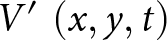 $V'\,\left( {x,y,t} \right)$ is the velocity anomaly at each spatial point and time,
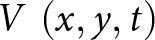 $V\,\left( {x,y,t} \right)$ is the individual velocity of each spatial point and time, and
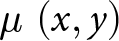 $\mu \,\left( {x,y} \right)$ is the mean velocity of each spatial point through 2015–24. We perform this operation for every pixel in the study area. We then calculated the mean velocity anomalies for each month across all years for both moulin-drained and crevassed areas by averaging
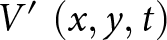 $V'\,\left( {x,y,t} \right)$ across all pixels in the area and across all observations that month.
Finally, to analyze the difference in seasonal velocity patterns across the two areas, we calculated the Z-scores of crevassed areas versus moulin-drained areas for each calendar month across the three elevation zones. We used the following equation for the Z-scores:
 \begin{equation}Z\, = \,\frac{{{\mu _{v{^{\prime}}c}}\, - \,\,\,{\mu _{v{^{\prime}}nc}}}}{{\sqrt {\frac{{\sigma _{v{^{\prime}}c}^2}}{{{N_{v{^{\prime}}c}}}} + \frac{{\sigma _{v{^{\prime}}nc}^2}}{{{N_{v{^{\prime}}nc}}}}} }}\end{equation}
Here, μv’c and μv’nc are the mean velocity anomalies of crevassed areas and moulin-drained areas, respectively, for a given calendar month over 2015–24, σv’c and σv’nc are the respective standard deviations, and Nv’c and Nv’nc are the respective number of velocity anomaly observations in each calendar month. Values of |Z| > 2.58 indicate a significant difference in velocity anomalies between crevassed and moulin-drained areas at 99% confidence. We computed 36 total Z-scores (12 months across three zones) and therefore we required a 99% confidence threshold instead of the typical 95% confidence threshold. Positive Z-scores denote crevassed areas experiencing higher velocity anomalies than moulin-drained areas, while negative Z-scores denote moulin-drained areas experiencing higher velocity anomalies than crevassed areas.
4. Results
Figure 7 shows the output of Model 6 for the presence of crevasse fields (green) and remnant supraglacial streams and lakes (blue) in the winter of 2020. On training data, the outputs from Model 6 scored 91% training accuracy, 21% training loss, 0.83 training mean IoU, 0.75 training IoU, 0.84 precision and 0.88 recall on crevassed areas at the final epoch of training. On validation data (cyan box, Fig. 7e), model outputs scored 85% validation accuracy, 19% validation loss, 0.75 validation mean IoU, 0.6 validation IoU, 0.75 precision and 0.75 recall on crevassed areas. These output metrics are listed in Supplementary Table S1. Figure 8 shows the manually classified and model-predicted crevasse fields and remnant supraglacial streams and lakes from validation region E in our study area. Cross-validation between the validation labels generated by the two individuals (Section 3.2) achieved an IoU score of 0.6 on crevassed areas.
Model 6 (Supplementary Table S1) detected crevasse field (green) and remnant stream/lake (blue) shapefiles overlain on the entire Pâkitsoq training region (divided into regions a–f). Purple boxes represent the training dataset of 20 subregions used to train the MimiNet model. Cyan box shows the validation dataset of four subregions used to validate model training at every epoch. Pink stars represent moulin locations over 2009–19 identified by Poinar and Andrews (Reference Poinar and Andrews2021).

Figure 7 Long description
The composite map displays the Pâkitsoq region divided into six subregions labeled a to f. Each subregion shows crevasse fields, streams/lakes and moulin locations. Crevasse fields are marked in green, with two types: WV-based labels and shaded labels. Streams and lakes are indicated in blue. Moulin locations, identified by Poinar and Andrews (2021), are marked with pink stars. Purple boxes represent training datasets, while cyan boxes indicate validation datasets. The map includes a scale bar of 5 kilometers for reference. Spatial distribution varies across subregions, with crevasse fields and streams/lakes appearing in clusters and isolated patches. Training and validation areas are clearly delineated, highlighting regions used for model development and testing.
(a) Manually classified labels of crevasse fields (green filled polygons) and streams/lakes (blue filled polygons) in region E of our study area. (b) Model predicted crevasse fields (green-outlined polygons) and streams/lakes (blue-outlined polygons) in region E of our study area. (c) Both the manually classified labels and the model predictions in region E are shown together.

Figure 8 Long description
Three thematic label (segmentation) maps show a study subregion labeled region E. No place names are shown. Orientation is not indicated. Legend used across the maps: crevasse field is shown with polygon symbols; stream or lake is shown with polygon symbols. In the validation map the polygons are filled; in the predicted map the polygons are outlines; in the overlay map both filled and outlined versions appear together. A) Validation input label. Filled polygons mark crevasse field areas and filled polygons mark stream or lake areas. A scale bar is shown. B) Predicted label. Outlined polygons mark crevasse field areas and outlined polygons mark stream or lake areas. A scale bar is shown. C) Overlay label. Filled and outlined polygons are shown together for both crevasse field and stream or lake areas. Several outlined polygons follow the edges of filled polygons and some outlined polygons appear where no filled polygon is present. A scale bar is shown.
After training and validation, our model identified a total area of 131 km2 covered by crevasse fields in Pâkitsoq in the winter of 2020. This represents 20% of the entire 629 km2 study area. Most (55%) of the crevassed area lies in large crevasse fields (sized 3.5 km2 or larger), whereas 45% of the crevassed area is in smaller regions. We found that region C, the highest-elevation area in the northeast quadrant of our study area, was the most heavily crevassed, with 33 km2 of crevassed area (31% of its total 105 km2 area). Remnant supraglacial streams and lake features identified in winter imagery accounted for a much smaller portion of the landscape, covering only 15 km2, or just 2% of the total area.
We also display locations of 32 moulins (Fig. 7) identified over 2009–19 by Poinar and Andrews (Reference Poinar and Andrews2021) in our study area. We found 30 of these previously identified moulins near our model-detected supraglacial streams and lake features, except one in region A next to a nunatak and one in region C on the edge of a crevasse field bordering with remnant supraglacial features.
4.1. Temporal persistence of crevasse field locations
We present our detections of crevasse fields and remnant supraglacial streams/lakes over 2015–24 for region E in (Fig. 9a–j). To assess the temporal variability in crevasse field locations, we define a ‘persistent crevasse field’ as a collection of pixels that our workflow identified as a crevasse field for at least 8 out of 10 years in the study period (Figs 11k and 12). We found that 60% of our total study area was either devoid of crevasse fields or occupied by crevasse fields detected for 2 years or less, 36% of our total study area had crevasses for at least 8 out of 10 years, and only 4% of our total study area was variable, with crevasses in 3–7 years. Essentially, all the crevasse fields we detected tend to occupy the same areas throughout the 2015–24 period studied. In sum, though the extent of crevassing varies from year to year, the spatial pattern is persistent.
(a–j) Model predictions of crevasse fields and remnant supraglacial streams/lakes in region E from 2015–24. (k) Map of persistent crevasse field detections over the 10 year study period in region E. Red shading denotes the total number of detections over 2015–24, with white meaning no detections and deep red meaning crevasse fields detected all 10 years. Yellow polygon outlines show crevasse fields detected by Hoffman and others (Reference Hoffman2018) in 2009–11. Violet polygons show crevasse detections by Chudley and others (Reference Chudley, Howat, King and MacKie2025) in 2016 from ArcticDEM 4.1 mosaics.

We compared persistent crevasse fields with the crevasse fields detected by Hoffman and others (Reference Hoffman2018) and Chudley and others (Reference Chudley, Howat, King and MacKie2025), which are outlined in yellow and violet (Figs 9k and 10), respectively. The Hoffman dataset contains 42 distinct crevasse fields, with a total crevassed area of 77 km2. Of those 42 crevasse fields, 39 directly coincide with crevasse fields in our dataset. In 34 of those, our crevasse fields were larger than the ones in Hoffman and others (Reference Hoffman2018), while three were smaller. Region E contains the two excluded crevasse fields that Hoffman and others (Reference Hoffman2018) digitized according to their study area bounds. The Hoffman and others (Reference Hoffman2018) crevasse fields from 2009–11 scored 0.7 mean IoU and 0.46 crevasse IoU against our persistent crevasse field dataset within their study area bounds. The Chudley dataset at 200 m resolution contains 22 crevasse fields in our study area, with a total crevassed area of 46 km2. Of those 22 crevasse fields, 17 coincide with crevasse fields in our dataset with partial to full coverage (see Section 5.4). Figure 11 shows the coverage of both 2 and 200 m crevasse detections in 2016 from Chudley and others (Reference Chudley, Howat, King and MacKie2025) in our study area. The Chudley and others (Reference Chudley, Howat, King and MacKie2025) crevasse fields from 2016 in Region D scored 0.66 mean IoU and 0.25 crevasse IoU against our persistent crevasse field dataset in the same region.
Map of persistence crevasse-field detections over the 10 year study period on the entire Pâkitsoq study area. Red shading denotes the total number of detections over 2015–24, with white meaning no detections and deep red meaning crevasse fields were detected in all 10 years. Yellow polygons show crevasse fields detected by Hoffman and others (Reference Hoffman2018) in 2009–11 for comparison. Violet polygons show crevasse detections by Chudley and others (Reference Chudley, Howat, King and MacKie2025) in 2016 from ArcticDEM 4.1 mosaics.

Figure 10 Long description
The map illustrates crevasse persistence over a 10-year period in the Pâkitsoq study area. Red shading indicates the number of detections from 2015 to 2024, with white representing no detections and deep red indicating crevasse fields detected all 10 years. Yellow polygons outline crevasse fields detected by Hoffman and others from 2009 to 2011, while violet polygons show detections by Chudley and others in 2016. The map is divided into six sections labeled a to f, each showing different areas of crevasse persistence. The legend specifies the count of years for crevasse persistence, with a scale bar indicating 5 kilometers for reference. Spatial distribution of crevasse fields is marked by clusters and corridors, with varying persistence levels across the sections.
Map of our study area MimiNet-detected crevasse fields (green) with individual regions labeled A–F (black rectangle) in Pâkitsoq, Greenland, showing MimiNet-detected crevasse fields (green) and 200 m crevasse fraction (red) by Chudley and others (Reference Chudley, Howat, King and MacKie2025) across the study area. Also shown are 2 m binary crevasse detections (purple) from Chudley and others (Reference Chudley, Howat, King and MacKie2025) across the entire view. Background image is the Sentinel-2 August 2019 median scene (MacGregor and others, Reference MacGregor, Fahnestock, Colgan, Larsen, Kjeldsen and Welker2020) and 500 m surface elevation contours from BedMachine v5 (Morlighem and others, Reference Morlighem2022).

Figure 11 Long description
Map of Pâkitsoq, Greenland, displaying MimiNet-detected crevasse fields in green and 200 m crevasse fraction in red, as identified by Chudley and others. The map also includes 2 m binary crevasse detections in purple across the entire view. Regions are labeled A–F within a black rectangle. The background is a Sentinel-2 August 2019 median scene, with 500 m surface elevation contours from BedMachine v5. The map provides a detailed view of crevasse distribution and elevation contours, with a scale bar indicating 2 kilometers. The coordinates and a north arrow are present for orientation.
4.2. Seasonal variability in ice flow
We investigated whether there is a difference in ice flow speed between crevasse fields and moulin-drained areas over the melt season. Figure 12 shows the monthly area-composited velocity anomalies over the melt season averaged over 2015–24. We also show the number of ITS_LIVE monthly velocity observations that passed our filtering criteria in (Fig. 13a). These numbers peak in the summer and become more sparse in the winter, when low solar illumination limits usable image acquisitions. The general ice flow direction is from the northeast to southwest. Figure 13a shows the monthly average velocity anomalies with ±1σ variance across our sample of N max = 470 observations (0.7% of the total unfiltered observations) over the 2015–24 study period. This large sample size allows only slight differences in the mean to be significant, even despite the large variance.
Monthly velocity anomalies of persistent (a) moulin-drained and (b) crevassed areas in the Pâkitsoq study area, showing the spatial variability of ice flow speedup through the melt season averaged over 2015–24. Previously identified moulin locations (purple stars) from Poinar and Andrews (Reference Poinar and Andrews2021) are shown in panel a. Dotted lines show the three elevation zones (from left to right): lower-elevation (∼500–750 m), mid-elevation (∼750–950 m) and higher-elevation (∼950–1100 m). (c) Histogram density plots of the monthly velocity anomalies of persistent moulin-drained (brown) and crevassed areas (green). Persistent moulin-drained and crevassed areas are defined as features detected over ≥8 of the 2015–24 study period.

Figure 12 Long description
The figure contains maps and histograms illustrating velocity anomalies in moulin-drained and crevassed areas from May to September. The maps show spatial variability with a color scale indicating velocity anomalies, where positive values represent speedup and negative values indicate slowdown. In the moulin-drained areas, May and June show higher anomalies, decreasing by September. Crevassed areas display similar trends but with less intensity. The histograms compare monthly velocity anomalies for both areas. The x-axis is labeled Velocity Anomaly in meters per year and the y-axis is Density. Moulin-drained areas are shown with one line style and crevassed areas with another. May shows broader distributions, while September narrows. Peaks are observed in May for moulin-drained areas, indicating higher anomalies compared to crevassed areas. The figure highlights seasonal changes and differences in velocity anomalies between the two area types.
(a) Velocity anomalies from 2015–24 averaged over moulin-drained areas (brown) and crevassed areas (green) in Pâkitsoq study area with ±1σ variance shaded, showing the temporal variability of ice flow speedup for January–December. Number of ITS_LIVE velocity observations of moulin-drained (brown) and crevassed areas (green) for January–December within velocity filtering criteria is shown below. (b) Z-scores of the monthly velocity anomalies of crevassed areas compared to moulin-drained areas from 2015–24 are shown for three approximate elevation zones: lower-elevation 500–750 m (blue), mid-elevation 750–950 m (violet) and higher-elevation 950–1100 m (magenta). Results within the cyan band (|Z| < 2.58) show no significant velocity difference between crevasse areas and moulin-drained areas, at 99% confidence. Positive Z-scores indicate that velocity anomalies are higher in crevassed areas than moulin-drained areas; negative Z-scores indicate the opposite.

Figure 13 Long description
The image A showing a scientific line plot with a legend listing Moulin-drained Areas and Crevassed Areas. The x-axis is labeled Month with tick labels Jan, Feb, Mar, Apr, May, Jun, Jul, Aug, Sep, Oct, Nov, Dec. The left y-axis is labeled Velocity Anomaly (m yr superscript -1) with labeled ticks at minus 150, minus 100, minus 50, 0, 50, 100, 150. Two lines run across the months with shaded bands around each line. Moulin-drained Areas line values by month are near minus 20 at Jan, near minus 30 at Feb, near minus 30 at Mar, near 20 at Apr, near 30 at May, near 60 at Jun, near minus 10 at Jul, near 0 at Aug, near 0 at Sep, near 30 at Oct, near 30 at Nov and near minus 20 at Dec. Crevassed Areas line values by month are near minus 20 at Jan, near minus 30 at Feb, near minus 30 at Mar, near 20 at Apr, near 30 at May, near 60 at Jun, near minus 10 at Jul, near 0 at Aug, near 0 at Sep, near 30 at Oct, near 30 at Nov and near minus 20 at Dec. A set of vertical bars appears along the bottom of the plot area. A right-side y-axis is labeled with ticks at 0, 235 and 470. The bars vary by month, with taller bars in mid-year months and shorter bars in early and late months. The image B showing a scientific line plot titled Velocity Anomalies (Crevassed vs Moulin-drained Areas). The x-axis is labeled Month with tick labels Jan, Feb, Mar, Apr, May, Jun, Jul, Aug, Sep, Oct, Nov, Dec. The y-axis is labeled Z-scores with labeled ticks at minus 5, 0, 5. Three lines are shown with a legend listing Lower Elevation (approx. 500-750m), Mid Elevation (approx. 750-950m) and Higher Elevation (approx. 950-1100m). Two horizontal reference lines are labeled z equals 2.58 and z equals minus 2.58. Lower Elevation line values by month are near 0 at Jan, near 0 at Feb, near 0 at Mar, near minus 3 at Apr, near minus 2 at May, near 0 at Jun, near 2 at Jul, near minus 2 at Aug, near minus 1 at Sep, near 0 at Oct, near 0 at Nov and near 1 at Dec. Mid Elevation line values by month are near 0 at Jan, near 0 at Feb, near 0 at Mar, near minus 2 at Apr, near minus 2 at May, near 0 at Jun, near 1 at Jul, near minus 2 at Aug, near minus 1 at Sep, near 0 at Oct, near 0 at Nov and near 0 at Dec. Higher Elevation line values by month are near 0 at Jan, near 0 at Feb, near 0 at Mar, near 1 at Apr, near 0 at May, near 2 at Jun, near 0 at Jul, near minus 2 at Aug, near 0 at Sep, near minus 1 at Oct, near minus 2 at Nov and near minus 2 at Dec.
In moulin-drained areas, ice flow undergoes a strong seasonal cycle from May through September, which coincides with the melt season. These areas experience an average velocity anomaly of 30 ± 68 m yr−1 in May, 57 ± 95 m yr−1 in June, −12 ± 63 m yr−1 in July, −3 ± 60 m yr−1 in August and 2 ± 41 m yr−1 in September. In crevasse fields, the seasonal pattern of ice flow is slightly different. Crevasse fields experience an average velocity anomaly of 27 ± 56 m yr−1 in May, 55 ± 90 m yr−1 in June, 4 ± 66 m yr−1 in July, − 2 ± 56 m yr−1 in August and 0 ± 41 m yr−1 in September. Both moulin-drained areas and crevasse fields experience the highest positive velocity anomalies in June, indicating a spatially pervasive spring-to-early-summer speedup for the entire region (Fig. 12c). Ice flow slows significantly in July in moulin-drained areas, while in crevassed areas, ice velocity remains above average. In both moulin-drained and crevassed areas, ice velocity slows down to pre-summer velocities through August and September.
Results of the velocity anomaly Z-test between crevassed and moulin-drained areas across the three approximate elevation zones are shown in Figure. 13b for all calendar months, averaged over 2015–24. Here, we report instances where the Z scores differed substantially from zero. In May, at middle elevations, the average velocity anomaly in crevassed areas was +15 m yr−1, which was lower (Z =−2.5) than what we observed in moulin-drained areas, +28 m yr−1. At lower and higher elevations, the change was not significant (Z = −1.7 and 1.9, respectively). In June, crevassed and moulin-drained areas at all elevations have high velocity anomalies that are not significantly different from one another. In July, lower-elevation crevassed areas slow down (−19 m yr−1) significantly less than moulin-drained areas (−42 m yr−1, Z = 4.8). At mid-elevations, crevassed areas experience nearly no change (−2 m yr−1) while moulin-drained areas slow down (−12 m yr−1); the difference is not significant (Z = 2.4). At higher elevations, no significant difference occurs (Z =− 0.8). In August, both areas at lower and middle elevations continue to slow down similarly (Z = 0.6 and Z = −1.8, respectively). At higher elevations, the average velocity anomaly in crevassed areas was +26 m yr−1, which is significantly lower (Z = −2.6) than what we observed in moulin-drained areas +44 m yr−1. In September, both crevassed and moulin-drained areas across all three elevation zones slow down to pre-summer speeds, showing near-zero velocity anomalies overall that are statistically indistinguishable in crevasse fields and moulin-drained areas. This marks the end of the melt season. Crevasse fields and moulin-drained areas experience similar velocity anomalies over winter from September through March.
4.3. Time evolution of total crevassed area in Pâkitsoq
We studied the time evolution in the total crevassed area of our study area in Pâkitsoq. Figure 14 shows crevasse detections from the eight MimiNet models described in Section 2.4. Figure 14a shows the total crevassed area observed each year over our 10 year study period (2015−2024), with error bars showing 1 sigma variations across the eight models. There is no overall trend over the study period (R 2 = 6 × 10⁻³, p = 0.838).
(a) Time evolution of crevassed area in Pâkitsoq, Greenland, over 2015–24 identified by eight MimiNet models. Green circles show the total crevassed area over time, with gray error bars showing the 1σ range across the results from the eight models. Green line shows the least-squares fit to the time series, with shaded green area showing the 95% confidence interval. Values of R 2 and p are shown. (b) Stacked histogram showing the total crevassed area over 2015–24, colored by year, detected by the eight models. Models trained on labels based on Sentinel-1 wintertime imagery are outlined in black, while models trained on labels based on WorldView summertime imagery are outlined in white.

Figure 14 Long description
A The horizontal axis label is Years (January minus April), with ticks from 2015 to 2024. The vertical axis label is Total crevassed area (km superscript 2), with ticks from 80 to 160. A legend lists Line of Fit and Crevassed Area. Points with vertical error bars are plotted for each year 2015 to 2024 and a fitted line with a shaded band is drawn across the series. The plotted points cluster in a narrow band across the years, with the lowest point around 2019 near 100 km superscript 2 and most other years around 115 to 135 km superscript 2. Text on the plot reads: R superscript 2 equals 6 times 10 superscript minus 3; p equals 0.838. b The horizontal axis label is Count, with ticks from 0 to 8. The vertical axis label is Total Crevassed Area (km superscript 2), with ticks from 80 to 160. A stacked horizontal bar chart shows multiple bars at different Total Crevassed Area values, with each bar divided into segments corresponding to the legend titled Year: 2015, 2016, 2017, 2018, 2019, 2020, 2021, 2022, 2023, 2024. The longest stacked bars occur around Total Crevassed Area near 140 to 150 km superscript 2, reaching counts close to 8, while shorter bars appear at lower values near 90 to 110 km superscript 2.
In the first year of our study period, 2015, we found a total crevassed area of 117 ± 5 km2. The maximum total crevassed area over our 10 year study period was 144 ± 6 km2 in 2016. The minimum occurred in 2019; at 106 ± 5 km2, it is substantially lower than the area in other years but is still within measurement uncertainty of the study period mean, 128 km2. We found that the overall standard deviation of the crevassed area was 11 km2.
Figure 14b summarizes the total crevassed area from 2015–24 calculated from the eight models. The stacked bars outlined in black show the results from the five models trained on labels based on Sentinel-1 wintertime imagery, while those outlined in white show the results from the model trained on labels based on WorldView summertime imagery (Section 3.4). These results are significantly different from each other. The five models operating on wintertime imagery produce consistent results between 110–160 km2, while the three models operating on summertime imagery find slightly lower crevassed areas, ranging from 80–130 km2 over the study period. This variability may be the result of the difference in seasons (winter versus summer), image resolution or differences in feature capture by the optical versus radar sensors. All models, whether using wintertime or summertime imagery, found that the highest crevassed area occurred in 2016 (orange, 13% above the mean) and the lowest crevassed area in 2019 (purple, 17% below the mean). This consistency between seasons and sensors gives further confidence in the accuracy of the model to identify crevasses on the ice surface and shows that there is consistently detectable interannual variability in the size of crevasse fields.
5. Discussion
5.1. Persistence in crevasse field locations
As demonstrated in Figs 9k and 10, MimiNet can identify the locations of crevasse fields from remote sensing imagery. With MimiNet, we were able to extend the crevasse fields identified by Hoffman and others (Reference Hoffman2018), who manually digitized crevasse fields from WorldView-1 optical imagery acquired in 2009–11, to the 2015–24 detections presented in this study. We find that the crevasse fields in Pâkitsoq largely occupied the same locations across the two studies, despite differences in the type of satellite imagery, detection methods and the 5 year time gap (2011–15) inherent to the two datasets. Generally, crevasses open at the same locations on the ice sheet surface where steep bed topography causes high extensional strain rates (Echelmeyer and others, Reference Echelmeyer, Clarke and Harrison1991; Cuffey and Paterson, Reference Cuffey and Paterson2010; Joughin and others, Reference Joughin2013). Both Hoffman and others (Reference Hoffman2018) and our results indicate this process. Slight differences in the locations of crevasse fields identified by Hoffman and others (Reference Hoffman2018) and by us could originate from differences in image geolocation, seasons of imagery acquisition, crevasse detection methods or from actual changes in crevasse field geometry. MimiNet detects a crevasse field based on the extent of the bright linear patch of crevasses on SAR imagery, while Hoffman and others (Reference Hoffman2018) results show generally smaller crevasse fields, with boundaries differing by a few hundred meters. This difference likely stems from the limitation of manual delineation of crevasse fields on optical imagery, where a crevasse may be obscured by snow cover, limiting visual identification at the margins of crevasse fields. MimiNet, which uses SAR imagery, is not limited by the presence of snow and can therefore be applied to imagery collected at any time of year. Fluctuations in the sizes of the crevasse fields are likely caused by the individual detection method (hand-digitizing versus deep learning) and satellite imagery type (optical versus radar), rather than indicating a change between 2009–24.
5.2. Absence of trend in Pâkitsoq crevassed area
Our 10 year study of the total crevassed area across Pâkitsoq, Greenland found interannual variability of −17% to +13% with no overall trend over the full time series (Fig. 14a). This lack of a trend over the 10 year observation period contrasts with Colgan and others (Reference Colgan2011), who found a significant increase in crevassed area of ∼33 km2 (5%) between 1985–2009 for a 608 km2 region that overlaps with and extends south of our area. A linear increase in crevasse area between 1985–2009 would correspond to an average increase of 1.37 km2 yr−1, or 0.2% of the study area per year. A significant advantage of our approach over this end-to-end comparison is the time series nature of our analysis, which yields a linear fit with uncertainties (Figure 14a) and provides a range of possible changes in crevassed area over our 2015–24 study period. The maximum rate of change allowed by the uncertainties on our fit is ±3.33 km2 yr−1 over our 629 km2 study area, or +0.5% of the study area per year. This is consistent with the +0.2% yr−1 found by Colgan and others (Reference Colgan2011), although we emphasize that our finding was no trend. Similarly, their finding of a 5% increase in crevassed area between two study years is well within our detected interannual variability of +13%.
In central western Greenland, Chudley and others (Reference Chudley, Howat, King and MacKie2025) found a significant decrease in crevassed area (−14%) between the 2 years 2016 and 2021. They inferred that crevasse fields experienced active closure within their 5 year study period due to the slowdown of Sermeq Kujalleq, which occurred in the latter half of the 2010s due to cooler oceanic temperatures (Khazendar and others, Reference Khazendar2019; Joughin and others, Reference Joughin, Shean, Smith and Floricioiu2020). The local decrease in crevassed area observed by Chudley and others (Reference Chudley, Howat, King and MacKie2025) would likely also affect our nearby study area as well (Colgan and others, Reference Colgan2011). If we were to subset our crevassed area time series so that only 2016 and 2021 are compared, mirroring Chudley and others (Reference Chudley, Howat, King and MacKie2025), we would also find a significant decrease in crevassed area (−9%), comparable to their −14% findings. Conversely, our time series would yield a significant increase in crevassed area (+14%) if we only compared 2015 and 2024. Therefore, our full time-series analysis is advantageous over previously published comparisons of individual years.
We can identify the trend in crevassed area that accounts for interannual variability, as shown in a previous remote sensing-based study on a different glacier (Van Wyk de Vries and others, Reference Van Wyk de Vries, Lea and Ashmore2023). Our findings in Pâkitsoq suggest that the crevasse extent in nearby Sermeq Kujalleq may also exhibit interannual variability. This interannual variability could explain the pattern of varying expansion and reduction of crevassed area observed in specific years over a 36 year period found by Colgan and others (Reference Colgan2011) and Chudley and others (Reference Chudley, Howat, King and MacKie2025), respectively. We speculate that two strong drivers likely influence the variability of crevassed area in this region: the effect of year-to-year variability of the ice flow regime (Van Wyk de Vries and others, Reference Van Wyk de Vries, Lea and Ashmore2023) and substantial changes in the crevassed extent of Sermeq Kujalleq driven by oceanic temperature changes (Khazendar and others, Reference Khazendar2019; Joughin and others, Reference Joughin, Shean, Smith and Floricioiu2020). In addition to that, intraregional variability in ice flow rates can stress the ice beyond its tensile strength in some years but not in others. These factors may contribute to the decreasing and increasing trends present through a range of years, such as 2016–19 and 2020–24, respectively. The year-to-year change in area of any single crevasse field is, however, not substantial as they are consistently forming in the same places on the ice sheet, just with larger or smaller size across years. Since we analyze winter scenes, it may be that a crevasse field is slower to open in some years while still attaining its full size in the melt season. The nature of our data acquisition prevents us from knowing this. Thus, continuous time series analysis of multiple years to decades is key to studying the trend and evolution of the crevassed area extents.
5.3. Spatial variability of ice flow and inferences about the subglacial hydrologic system
We interpret the seasonal velocity patterns we observe in our study area in terms of the contrasting roles of moulins and crevasse fields in bringing meltwater to the ice-sheet bed. Moulins drain meltwater from large catchments that can exceed ∼16 km2 (Mejia and others, Reference Mejia2022) and deliver it to the bed at discrete locations. This delivery occurs quickly and relatively early in the melt season, allowing localized channels to form in the subglacial drainage system during June (Banwell and others, Reference Banwell, Willis and Arnold2013, Reference Banwell, Hewitt, Willis and Arnold2016) and persisting through at least August (Trunz and others, Reference Trunz2023). In contrast, moulins are almost entirely absent from all crevassed areas we identified (Fig. 7; Poinar and Andrews, Reference Poinar and Andrews2021). While some moulin-like drainage is observed in supraglacial stream-terminating crevasse fields in southwestern Greenland (Smith and others, Reference Smith2015), this phenomenon is absent in our study area. Thus, the subglacial system there should lack the concentrated water influxes that drive the subglacial system to quickly channelize. If the closely spaced crevasses within a crevasse field do deliver water to the bed, each individual crevasse would have a much smaller catchment than a moulin and would deliver only a small fraction of the meltwater volume compared to a moulin. We estimate that with characteristic crevasse spacing of ∼50 m in Pâkitsoq (Poinar, Reference Poinar2015) and length ∼300 m (Fig. 1b,c), the catchment size of each crevasse (∼0.015 km2) is one to three orders of magnitude smaller than that of a typical moulin (∼0.2–16 km2, Mejia and others, Reference Mejia2022). Therefore, a subglacial water flux through a single crevasse should be insufficient to develop a channelized drainage system under 700 m thick ice (Dow and others, Reference Dow, Kulessa, Rutt, Doyle and Hubbard2014). Thus, if crevasses do deliver water to an inefficient drainage system at the bed, we would expect ice flow speeds to be relatively faster over the mid-to-late melt season because these meltwater inputs would increase pressures within the inefficient subglacial system. While ice flow speeds can affect crevassed extents on glaciers (Zheng and others, Reference Zheng, Pritchard, Willis and Stearns2019), we focus on crevasse fields affecting ice speedups by carrying meltwater to the bed. MimiNet results show that there is year-to-year variability in the boundaries of crevasse fields by a few hundred meters, however, insufficient to drive substantial changes in year-to-year ice velocity. If crevasses do not convey meltwater to the bed, we would instead expect ice flow speeds within crevasse fields to be very similar to those in moulin-drained areas, following the ice-sheet coupling length of 3–8 ice thicknesses (Gudmundsson, Reference Gudmundsson2003), which is ∼5 km in our study area. We use our findings to evaluate this general hypothesis.
We interpret the temporal variability in ice flow speed Figure 13 in terms of surface meltwater availability and the implied evolution of the subglacial drainage system. Each of the ten melt seasons had different timing, which limits the ability of our long-term average month-by-month to resolve specific speedups. The onset of the melt season in this region typically occurs from May to early June (Wang and others, Reference Wang, Sharp, Rivard and Steffen2007; Andrews and others, Reference Andrews2014; Mejia and others, Reference Mejia2021). From May to June, the entire study area experiences substantial ice-flow speedup. In the moulin-drained portions of the study area, moulins develop by early June and begin to transport large amounts of meltwater to the distributed subglacial system (Morriss and others, Reference Morriss2013; Fitzpatrick and others, Reference Fitzpatrick2014; Andrews and others, Reference Andrews2018; Williamson and others, Reference Williamson, Banwell, Willis and Arnold2018; Poinar and Andrews, Reference Andrews2021; Mejia and others, Reference Mejia2022). In crevassed areas, the velocity anomaly data imply that crevasses also begin to transport meltwater to the bed in June, but that the subglacial hydrologic system remains in a distributed state.
In July, the velocity data show slowing ice flow speeds when compared to June (Figs 12 and 13), implying that meltwater across the moulin-drained areas continues to reach a channelized subglacial system (Koziol and Arnold, Reference Koziol and Arnold2018). Crevassed areas likely also continue to deliver meltwater to the bed; however, the water volume flux through the thousands of individual crevasses in our study area is inadequate to form subglacial channels, leaving the subglacial system in a distributed state. We infer that in July, decreasing surface melt rates cause the subglacial channels to begin shrinking. Therefore, while moulins in moulin-drained areas continue to deliver meltwater to the bed through August, the reduced volume of the channelized drainage system allows ice flow speeds to rise, while still remaining slower than peak summer (Fig. 12a,c, comparing August–June). Decreasing surface melt rates imply that crevassed areas receive less meltwater flux compared to peak melt in June and July, and the subglacial system remains in a distributed state, allowing stable ice flow rates in crevassed areas. Our analysis does not account for the ice-sheet coupling length, limiting our confidence in whether all crevassed areas in our study area deliver meltwater to the subglacial system.
5.4. Comparison to other fracture detection methods
While MimiNet does not detect individual crevasses, it is unique in that it can detect crevasse fields, along with supraglacial lakes and remnant streams from winter and early spring Sentinel-1 SAR imagery. Recent automated fracture detection studies have been able to locate individual fractures on Antarctic ice shelves (Lai and others, Reference Lai2020; Zhao and others, Reference Zhao, Liang, Li, Duan and Liang2022; Surawy-Stepney and others, Reference Surawy-Stepney, Hogg, Cornford and Hogg2023). The key difference is the size of the fractures being observed. Individual fractures on ice shelves can be hundreds of meters to multiple kilometers wide, making their individual detection in imagery feasible, even in low- or moderate-resolution imagery such as MODIS-based mosaics for Antarctica at 250 m resolution (Lai and others, Reference Lai2020). The kilometer-scale size of a single fracture on Antarctic ice shelves is comparable to the broad-scale output of MimiNet for Greenland: crevasse fields with dimensions of ∼1–5 km. These size differentials make it difficult to achieve single-crevasse detection on the ablation zone in Greenland from moderate-resolution imagery, although Van Wyk de Vries and others (Reference Van Wyk de Vries, Lea and Ashmore2023) achieved this through image processing algorithms.
MimiNet complements existing crevasse detection methods that have been optimized for the Greenland ice sheet margin (Van Wyk de Vries and others, Reference Van Wyk de Vries, Lea and Ashmore2023; Chudley and others, Reference Chudley, Howat, King and MacKie2025). Van Wyk de Vries and others (Reference Van Wyk de Vries, Lea and Ashmore2023) employ the Gabor crevasse detector (GCD) method to identify individual crevasses from Sentinel-2 optical imagery with 10 m spatial resolution on Narsap Sermia in southwestern Greenland. The method employed by Chudley and others (Reference Chudley, Howat, King and MacKie2025) uses DEMs produced from high-resolution optical imagery to detect individual crevasses with a minimum width and depth of 10 m. MimiNet detects crevasse fields composed of crevasses with a minimum width that we estimate at half of a Sentinel-1 SAR image pixel, or ∼5 m. Due to being trained with SAR imagery, MimiNet is not limited by daylight or cloud conditions and has new image acquisitions regularly; optical-imagery-based DEMs do not have these advantages. Both GCD and DEM-based methods excel at detecting individual, large crevasses, which are most often found on fast-flowing outlet glaciers or near ice-sheet margins. The DEM-based method of Chudley and others (Reference Chudley, Howat, King and MacKie2025) is able to detect crevasses with widths greater than approximately 10 m. In our study area, this equates to an approximate elevation limit of 850 m (Fig. 11): a substantial fraction of crevasses inland of this limit in our study area are too narrow for the DEM-based method to detect. MimiNet complements this with its ability to detect crevasse fields composed of narrower crevasses, which are typically found farther inland. However, MimiNet is limited from distinguishing individual open and relict crevasses on a crevasse field. Indeed, the crevasse detections in Pâkitsoq by Chudley and others (Reference Chudley, Howat, King and MacKie2025) are primarily below 900 m a.s.l., whereas MimiNet finds crevasse fields that extend ∼15 km farther inland, reaching the upper limit of our study area at 1100 m a.s.l. Chudley and others (Reference Chudley, Howat, King and MacKie2025) find isolated crevasses at 900–1100 m a.s.l., however, we find that many of those detections are better aligned with MimiNet-detected streams than with crevasse fields. This is consistent with the rough sizes of these features: higher-elevation crevasses are likely to be narrow (5–10 m), whereas streams can range from 1–30 m wide in this region (Yang and Smith, Reference Yang and Smith2013). This suggests the DEM method by Chudley and others (Reference Chudley, Howat, King and MacKie2025) may be detecting eroded supraglacial stream channels, not crevasses, above 900 m a.s.l. With weather-independent high-resolution SAR imagery, MimiNet makes it possible to locate crevasse fields throughout the ablation zone.
6. Conclusion
We provide the first deep-learning CNN-based automated crevasse detection from Sentinel-1 SAR imagery suitable for Greenland: MimiNet, a TensorFlow-based CNN model that runs on Ghub. In applying the MimiNet workflow to study the interannual variability in the locations and size of the crevassed areas in Pâkitsoq, central western Greenland. We found no overall trend in the crevasse extent over 2015–24, contrasting the decreasing trend in crevassed area previously identified in the region (Chudley and others, Reference Chudley, Howat, King and MacKie2025). The size and locations of crevasse fields were highly persistent over our 10 year study period, in agreement with a previous work (Hoffman and others, Reference Hoffman2018). Throughout our study period, we identified some seasonal velocity signals with a spring speedup in June and slowdown that occurred through August and September of each year. By using flow speed anomalies as a window onto the efficiency of the subglacial drainage network, we infer that crevasse fields in Pâkitsoq deliver meltwater to the bed but while moulin-drained areas are better able to efficiently route meltwater directly to the bed and drive seasonal changes in the subglacial drainage system structure and efficiency. Our workflow enables future research to study the spatial distribution and temporal trends in crevasse fields on ice masses surveyed by the Sentinel-1 satellite constellation. We envision that the improvement of SAR-despeckling techniques will lead to highly accurate crevasse detection results. Continuous mapping of crevasses will be beneficial to study the changing ice dynamics of both slow-moving and fast-moving glaciers on the Greenland ice sheet.
Supplementary material
The supplementary material for this article can be found at https://doi.org/10.1017/jog.2026.10185.
Data availability statement
The workflow for crevasse field detection in Pâkitsoq, Greenland, is available on Zenodo (https://doi.org/10.5281/zenodo.15116011) as well as accessible as a Ghub Tool (https://theghub.org/resources/crevassedetect).
Acknowledgements
This work was supported by NASA award 80NSSC19K0054 (Kristin Poinar) and NSF award 2004826 (Jason Briner, Sophie Nowicki and Kristin Poinar). Computing resources for this work were supplied and supported by the University at Buffalo’s Center for Computational Research (CCR).
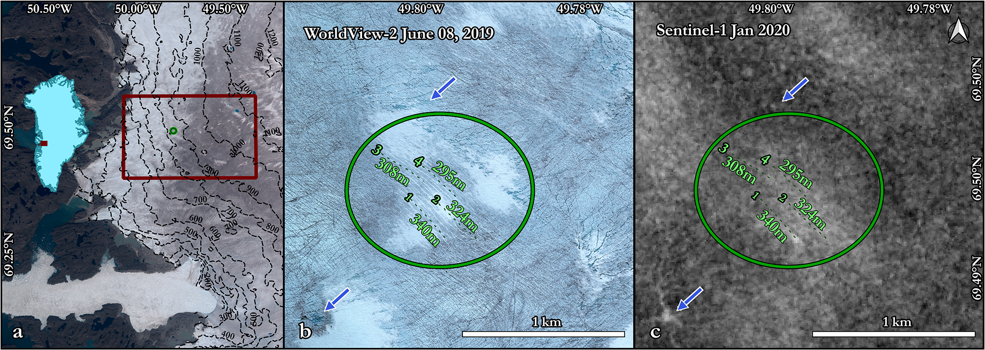
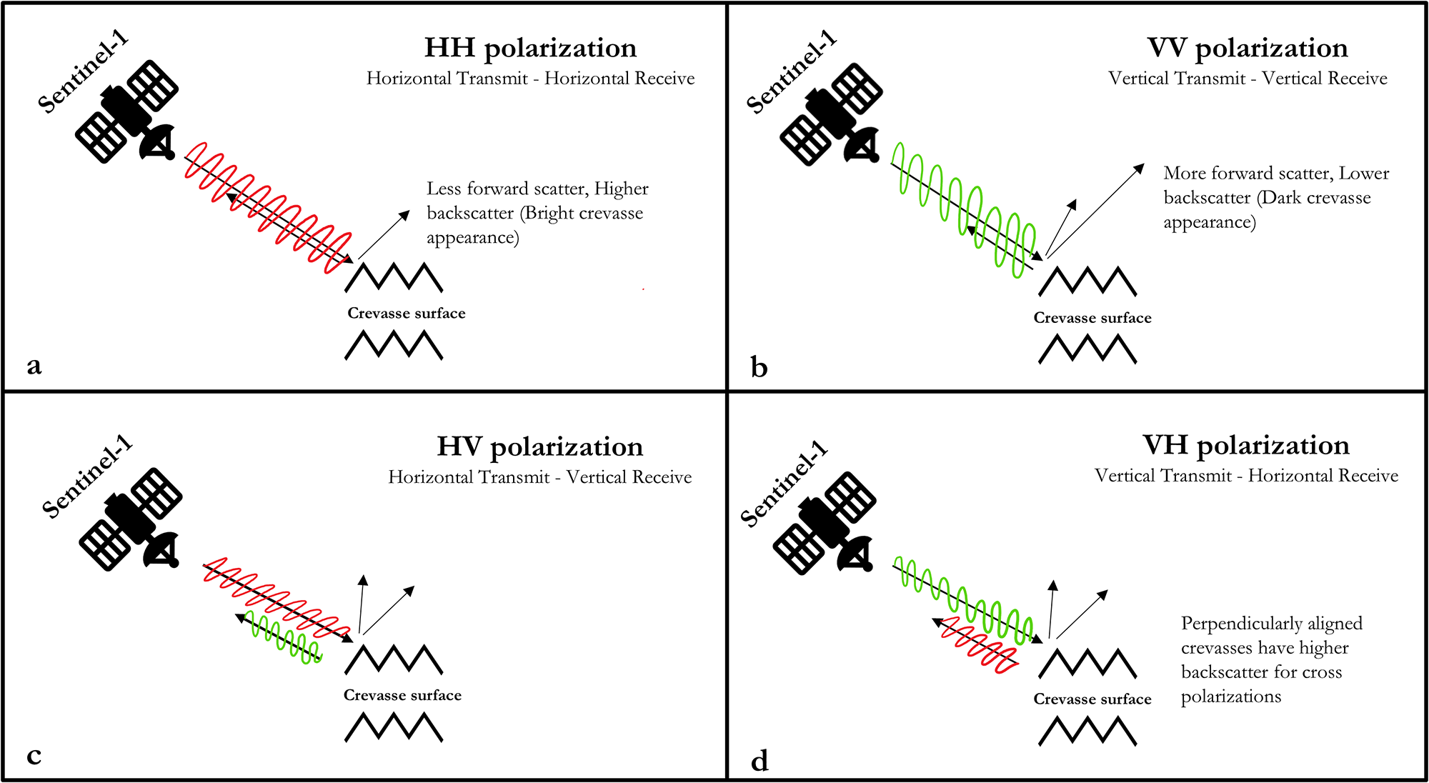
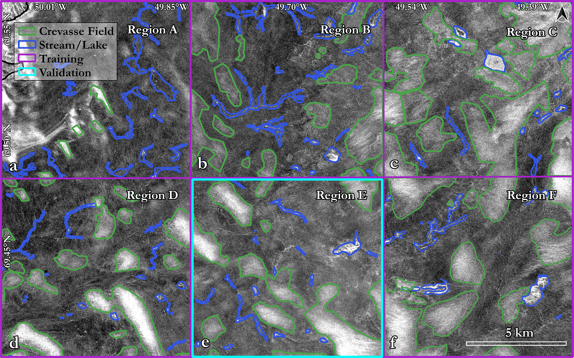
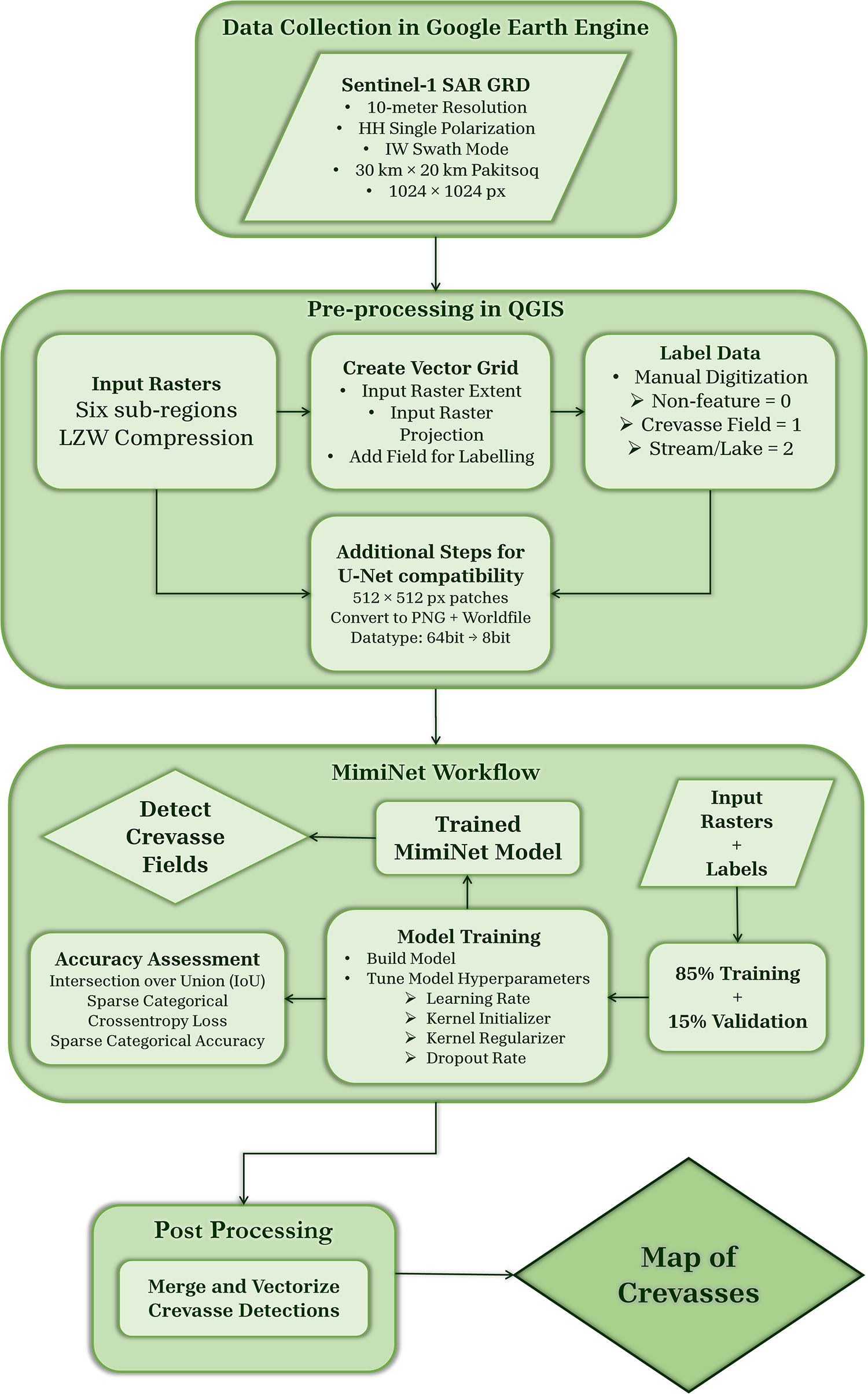
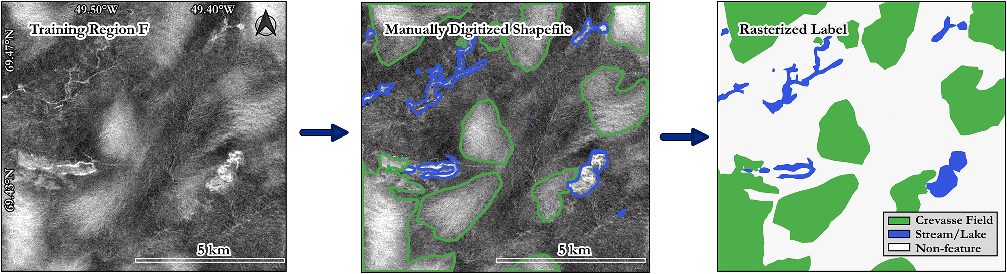
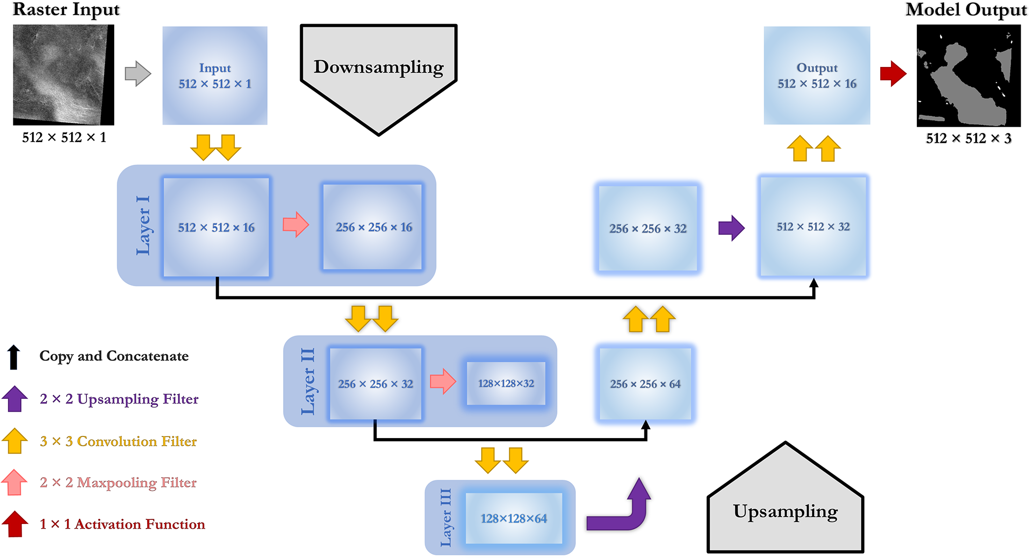
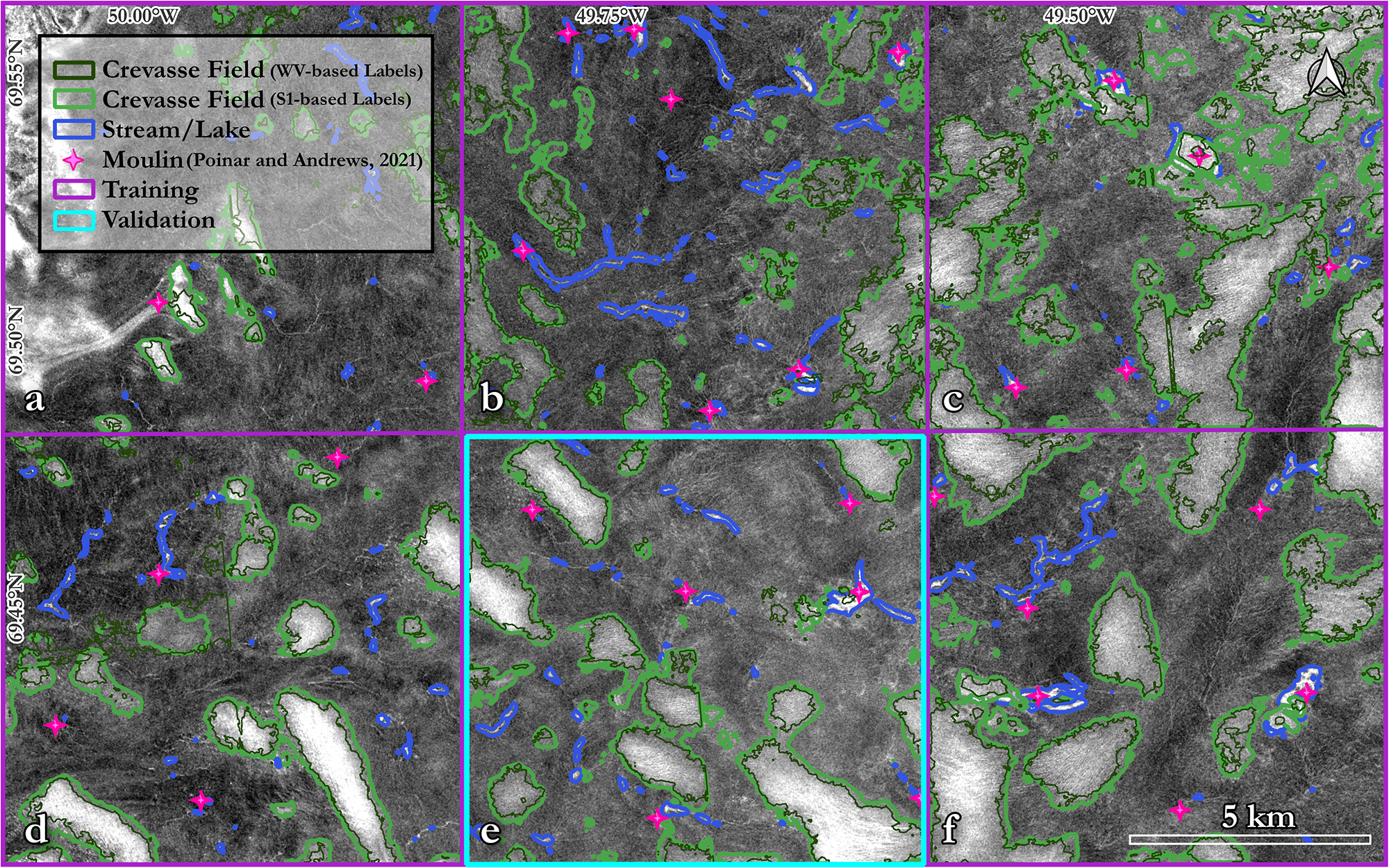
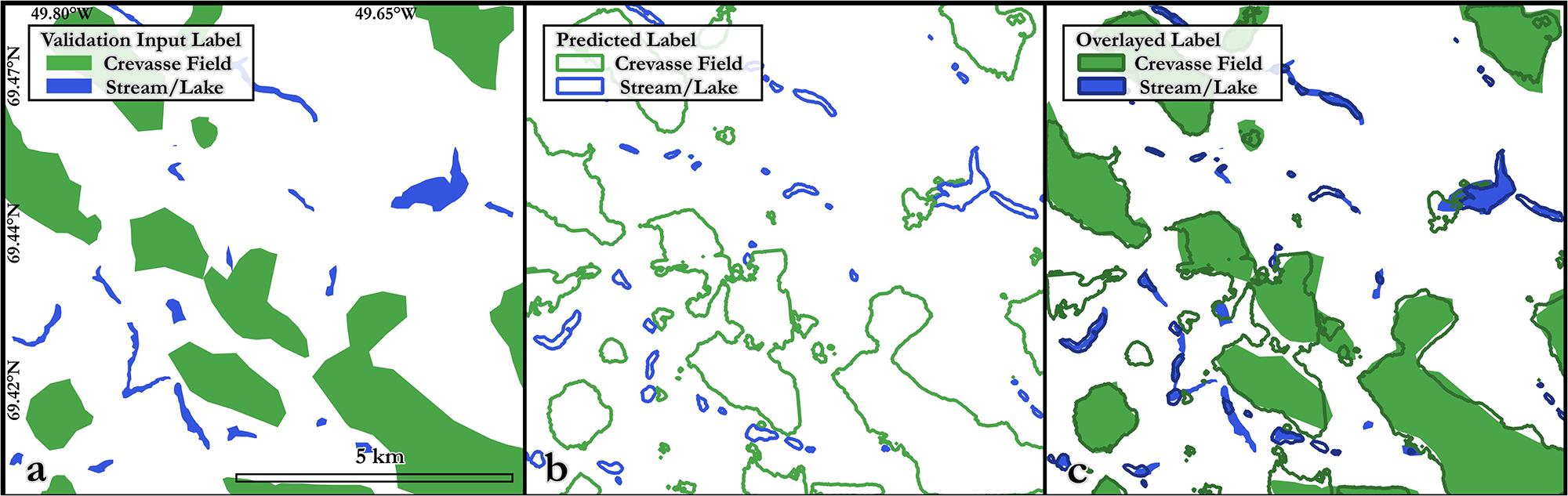
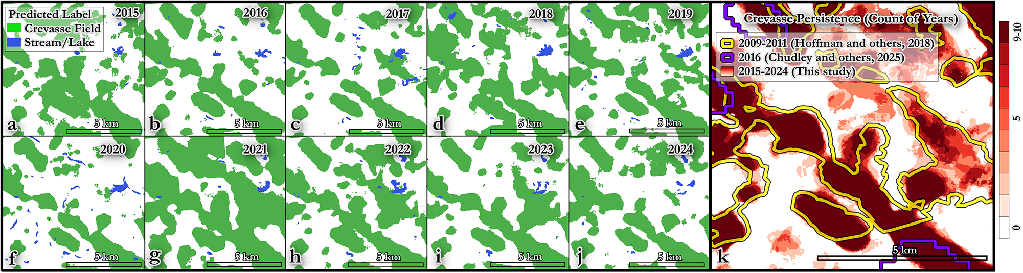
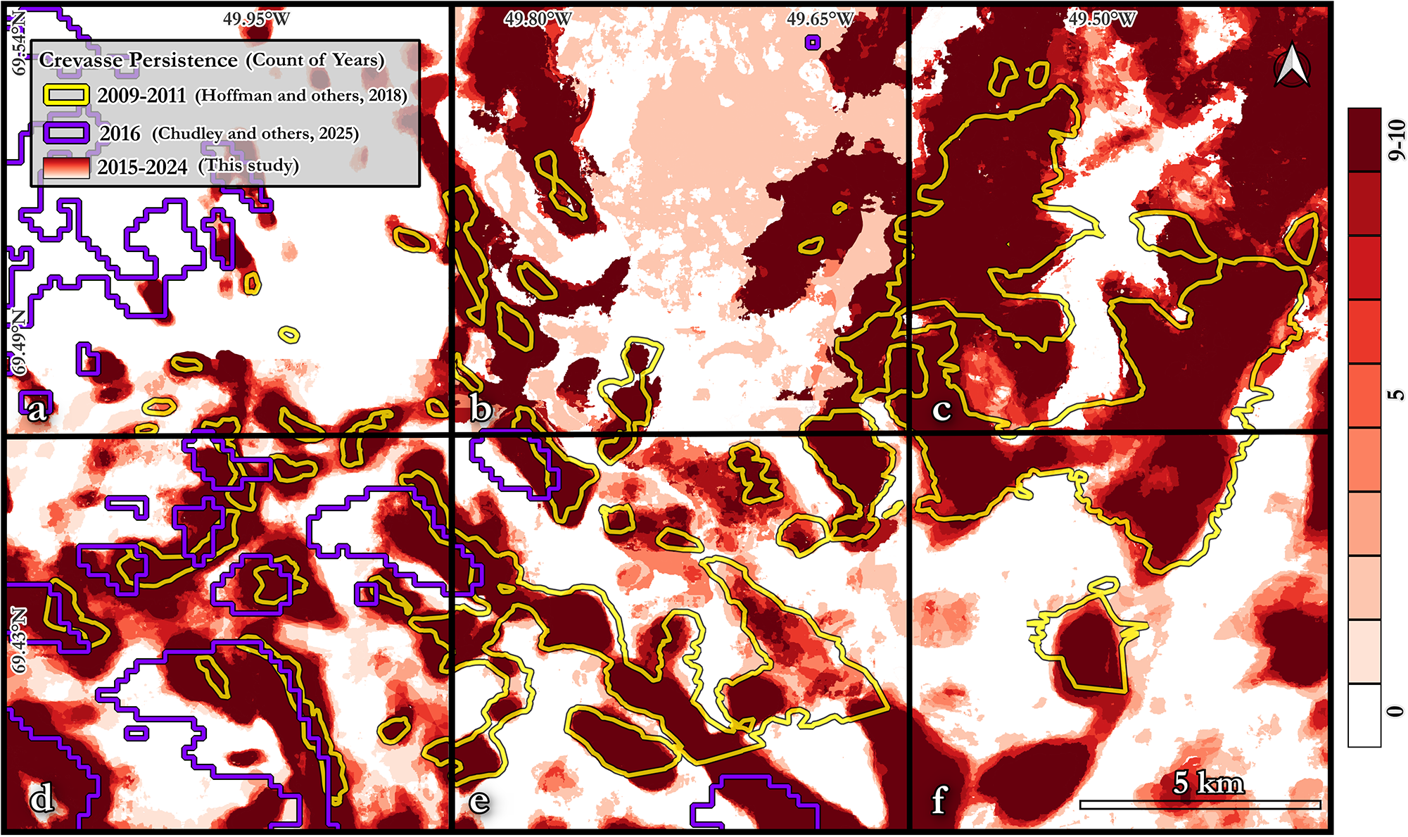
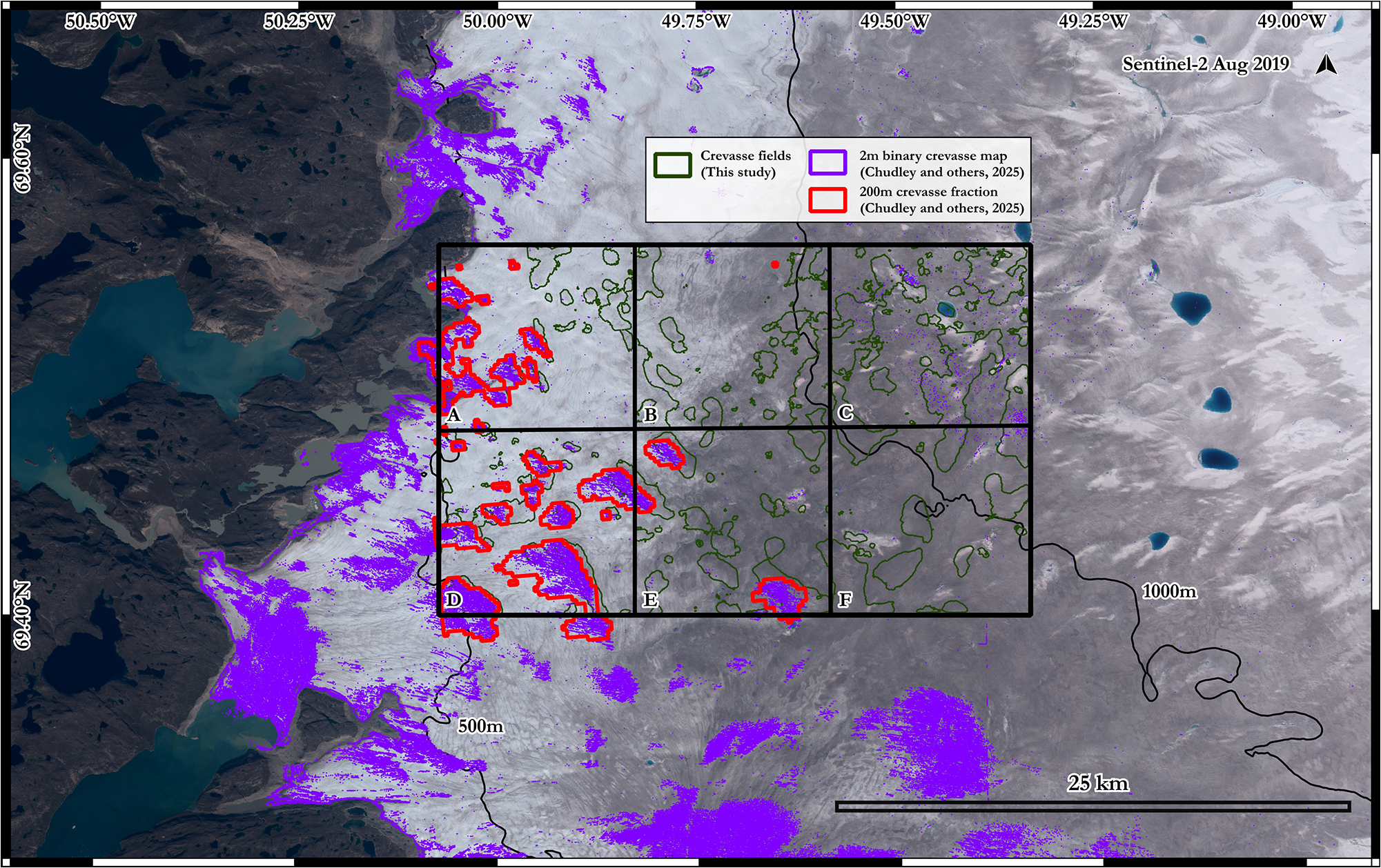
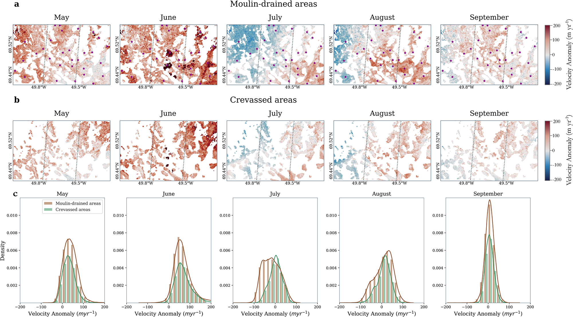
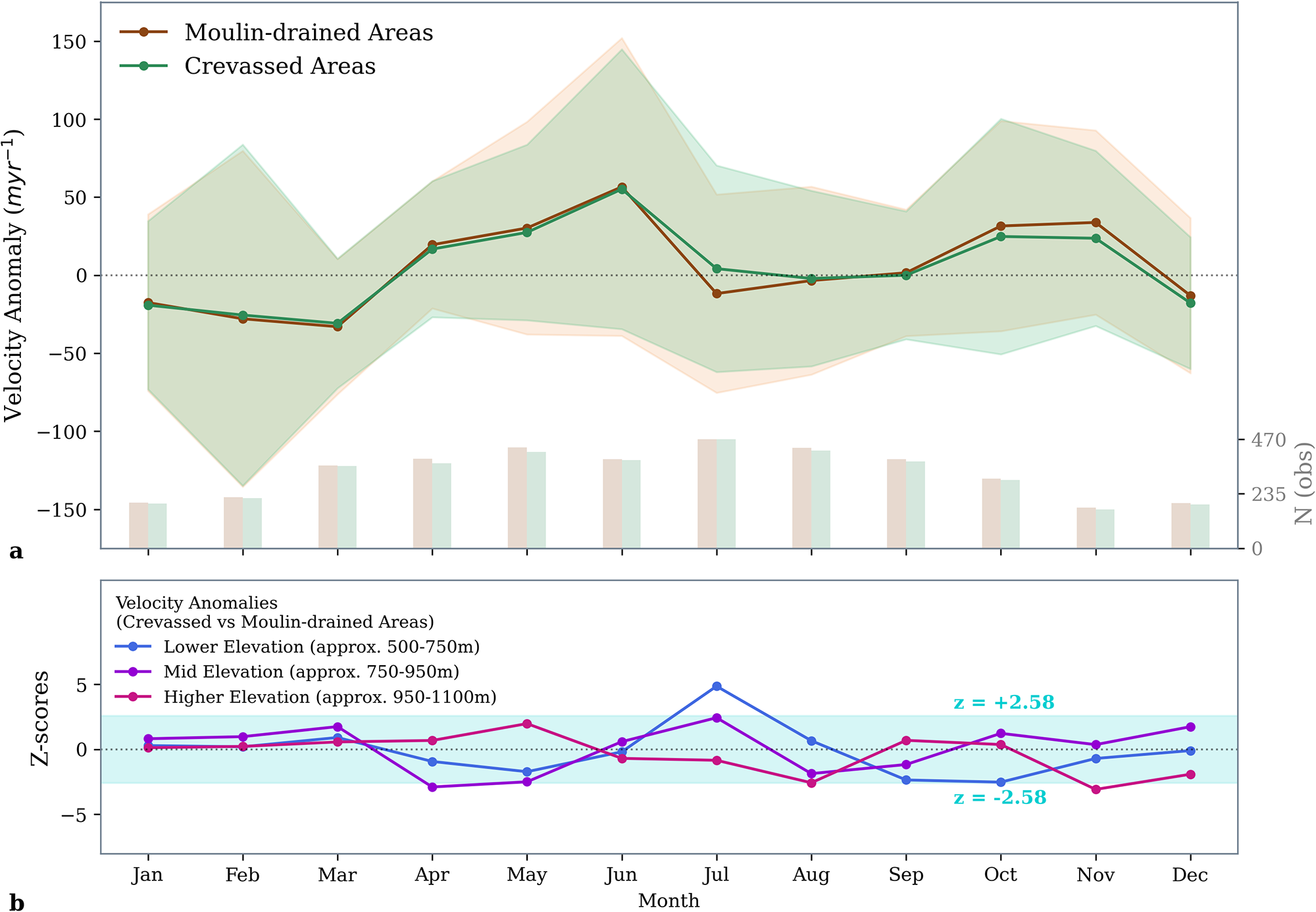
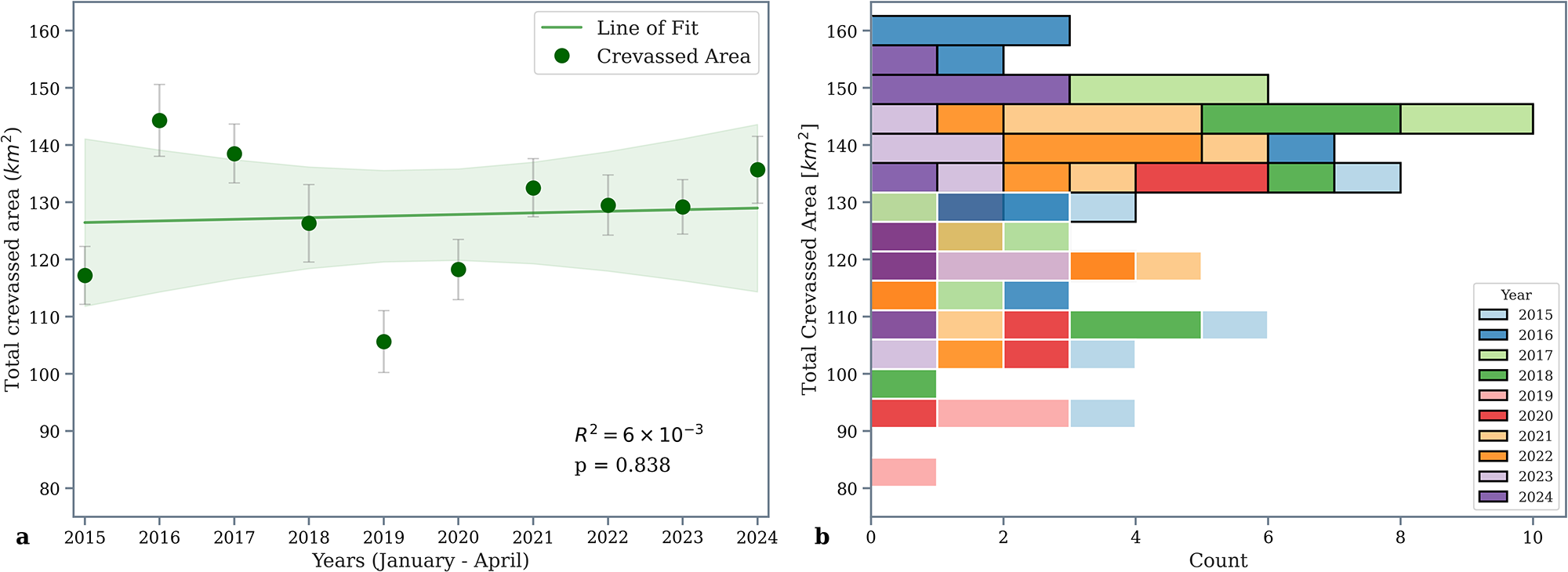


 Open access

