



1 Introduction
It is widely accepted that if the initial perturbations are small, the initial phase of the laminar–turbulent transition in wall-bounded shear flows is largely governed by linear mechanisms (Butler & Farrell Reference Butler and Farrell1992; Trefethen et al.
Reference Trefethen, Trefethen, Reddy and Driscoll1993; Schmid & Henningson Reference Schmid and Henningson2001; Jovanovic & Bamieh Reference Jovanovic and Bamieh2005). The application of linear control theory to fluid flows is therefore considered as a viable route to suppress instabilities and delay transition for reducing skin-friction drag (Joshi, Speyer & Kim Reference Joshi, Speyer and Kim1997; Bewley & Liu Reference Bewley and Liu1998; Cortelezzi & Speyer Reference Cortelezzi and Speyer1998; Högberg, Bewley & Henningson Reference Högberg, Bewley and Henningson2003a
; Baramov, Tutty & Rogers Reference Baramov, Tutty and Rogers2004; Chevalier et al.
Reference Chevalier, Hœpffner, Åkervik and Henningson2007; Bagheri, Brandt & Henningson Reference Bagheri, Brandt and Henningson2009b
; Semeraro et al.
Reference Semeraro, Bagheri, Brandt and Henningson2013; Jones et al.
Reference Jones, Heins, Kerrigan, Morrison and Sharma2015). In particular, optimal multivariable control strategies (LQG/
 ${\mathcal{H}}_{2},{\mathcal{H}}_{\infty }$
, where LQG denotes linear quadratic Gaussian) (Zhou, Doyle & Glover Reference Zhou, Doyle and Glover1996; Skogestad & Postlethwaite Reference Skogestad and Postlethwaite2005) have been successfully applied, see Kim & Bewley (Reference Kim and Bewley2007), Bagheri & Henningson (Reference Bagheri and Henningson2011), Sipp & Schmid (Reference Sipp and Schmid2016) for an in-depth review on this subject. These control strategies can be decomposed in a state estimation problem from non-ideal (noisy) measurements and a state feedback control problem. Once the evolution of the flow perturbations is sufficiently estimated, the estimated state can subsequently be used for feedback control of the perturbations. The construction of an accurate linear state-space model describing the perturbation dynamics from all inputs to all outputs is the cornerstone of linear model-based control and is considered as a significant challenge (Bagheri & Henningson Reference Bagheri and Henningson2011; Sipp & Schmid Reference Sipp and Schmid2016). Limits related to unmodelled dynamics and nonlinearities are commonly assessed from case to case (Semeraro et al.
Reference Semeraro, Bagheri, Brandt and Henningson2013; Fabbiane et al.
Reference Fabbiane, Simon, Fischer, Grundmann, Bagheri and Henningson2015) and/or addressed using robust design techniques such as
 ${\mathcal{H}}_{\infty }$
loop shaping (Jones et al.
Reference Jones, Heins, Kerrigan, Morrison and Sharma2015; Flinois & Morgans Reference Flinois and Morgans2016). For example, in Jones et al. (Reference Jones, Heins, Kerrigan, Morrison and Sharma2015) the effect of nonlinearity is attenuated by a linear feedback controller that employs high loop gain over a selected frequency range. As recently reviewed in Schmid & Sipp (Reference Schmid and Sipp2016), Sipp & Schmid (Reference Sipp and Schmid2016), different difficulties arise for modelling and control of globally unstable oscillator flows and convectively unstable amplifier flows. Oscillator flows, such as bluff body flows and open cavity flows, are characterised by the presence of global instabilities that oscillate at a particular frequency and are rather insensitive to upstream perturbations. Modelling the external disturbance environment is thus less of an issue for suppressing global instabilities (Samimy et al.
Reference Samimy, Debiasi, Caraballo, Serrani, Yuan, Little and Myatt2007; Barbagallo, Sipp & Schmid Reference Barbagallo, Sipp and Schmid2009; Ma, Ahuja & Rowley Reference Ma, Ahuja and Rowley2011; Sipp & Schmid Reference Sipp and Schmid2016), but it raises different issues related to nonlinear saturation of global instabilities (Flinois & Morgans Reference Flinois and Morgans2016). On the other hand amplifier flows, such as channel flows and boundary layer flows, are characterised by the presence of convective instabilities that amplify downstream (in space) in a broadband frequency spectrum in both space and time. Amplifier flows are highly sensitive to external disturbances and there exists only a small window in time to suppress convective instabilities. This poses great challenges for control design and accurately modelling the upstream disturbance environment is crucial since it forms the basis for estimation and control of the flow perturbations (Hœpffner et al.
Reference Hœpffner, Chevalier, Bewley and Henningson2005; Bagheri et al.
Reference Bagheri, Brandt and Henningson2009b
; Semeraro et al.
Reference Semeraro, Bagheri, Brandt and Henningson2011). This paper focuses on convective instabilities due to their strong relevance to engineering problems such as laminar–turbulent transition of flow over aerofoils. Besides the distinction in instability behaviour, two approaches with regard to the flow modelling and the controller synthesis are frequently further distinguished from each other (Bagheri & Henningson Reference Bagheri and Henningson2011), namely the wavenumber approach for distributed control design and the localised control approach using reduced-order models. The framework presented in this paper is inspired by both approaches, which are discussed next.
1.1 Distributed control and localised computations
A large number of studies, including the seminal works by Joshi et al. (Reference Joshi, Speyer and Kim1997) and Bewley & Liu (Reference Bewley and Liu1998), consider full-domain distributed sensing and actuation to derive the control laws. Distributed control designs often exploit the spatial invariance property of parallel flows to derive low-order models of the perturbation dynamics. In the case of spatial invariance it is assumed that the base flow is invariant in the streamwise (
 $x$
) and spanwise (
 $z$
) directions and that the sensors and actuators are fully distributed along these coordinates. By using a Fourier–Galerkin decomposition or a Fourier transform along the spatially invariant coordinates, the system can be block diagonalised and decoupled in terms of discrete sets of wavenumbers that replace the spatially invariant coordinates (Joshi et al.
Reference Joshi, Speyer and Kim1997; Bewley & Liu Reference Bewley and Liu1998). Analysis and design of the controller can thus be carried out on a parameterised lower-dimensional system. The resulting feedback controllers can subsequently be reconstructed in physical space by computing the so-called control convolution kernels (Bamieh, Paganini & Dahleh Reference Bamieh, Paganini and Dahleh2002; Högberg et al.
Reference Högberg, Bewley and Henningson2003a
). In Hœpffner et al. (Reference Hœpffner, Chevalier, Bewley and Henningson2005), Chevalier et al. (Reference Chevalier, Hœpffner, Bewley and Henningson2006) stochastic models for external sources of excitation were introduced that allow the computation of well-resolved estimation convolution kernels for shear stress and pressure measurements. These estimation/control convolution kernels have a localised structure in space and it was shown in Bamieh et al. (Reference Bamieh, Paganini and Dahleh2002) that localisation of the convolution kernels is a universal property of spatially invariant optimal control problems. Although, strictly speaking the wavenumber approach is only applicable to spatially invariant systems, it has also been successively applied to spatially developing boundary layers (Högberg & Henningson Reference Högberg and Henningson2002; Chevalier et al.
Reference Chevalier, Hœpffner, Åkervik and Henningson2007; Monokrousos et al.
Reference Monokrousos, Brandt, Schlatter and Henningson2008) and fully turbulent flows (Lee et al.
Reference Lee, Cortelezzi, Kim and Speyer2001; Högberg, Bewley & Henningson Reference Högberg, Bewley and Henningson2003b
; Sharma et al.
Reference Sharma, Morrison, McKeon, Limebeer, Koberg and Sherwin2011). The use of control/estimation convolution kernels avoids the need for online fast Fourier transforms (FFT) of the measurement vector and inverse fast Fourier transform (iFFT) of the control vector. While this approach introduces a controller with the same order as the system, it is shown in Högberg et al. (Reference Högberg, Bewley and Henningson2003a
) that spatially truncating the convolution kernels does not degrade the closed-loop performance of the control system. Since these convolution kernels are localised, the feedback controller can be implemented with only localised computations. As a result, relatively small computational domains can be considered for an effective control design. For example in Chevalier et al. (Reference Chevalier, Hœpffner, Åkervik and Henningson2007) and Monokrousos et al. (Reference Monokrousos, Brandt, Schlatter and Henningson2008) all perturbations were generated upstream of the control domain and they were able to suppress Tollmien–Schlichting waves and streaks in a flat plate boundary layer using small strips of distributed sensors and actuators.
1.2 Model reduction and localised control
The exploitation of the spatial invariance property for control design, although effective for distributed feedback control, requires sensor and actuator distributions that are currently not available or cannot be manufactured in a cost effective way. Moreover, in practice efficient control can be achieved using only a few localised sensors and actuators, leading to a more cost-effective control design. This led to the use of reduced-order modelling techniques for control design that make no assumptions on the flow geometry and the shape and distribution of the actuators/sensors. This approach, also known as the reduced-order modelling approach, accounts for physically realisable localised actuators/sensors and has been validated in experiments (Samimy et al. Reference Samimy, Debiasi, Caraballo, Serrani, Yuan, Little and Myatt2007; Pastoor et al. Reference Pastoor, Henning, Noack, King and Tadmor2008; Fabbiane et al. Reference Fabbiane, Simon, Fischer, Grundmann, Bagheri and Henningson2015). Galerkin projection is commonly applied, in which a reduced-order model (ROM) is obtained by projecting the Navier–Stokes equations onto a reduced set of modes. The choice of these modes is critical and greatly determines the effectiveness of the ROM for control application (Ilak & Rowley Reference Ilak and Rowley2008; Bagheri et al. Reference Bagheri, Henningson, Hoepffner and Schmid2009c ; Barbagallo et al. Reference Barbagallo, Sipp and Schmid2009). The global eigenfunctions of the linear operator (Åkervik et al. Reference Åkervik, Hoepffner, Ehrenstein and Henningson2007), as well as different variants of proper orthogonal decomposition modes (POD) (Noack et al. Reference Noack, Afanasiev, Morzynski, Tadmor and Thiele2003; Siegel et al. Reference Siegel, Seidel, Fagley, Luchtenburg, Cohen and McLaughlin2008) have been successfully applied for model reduction and control design. Another approach is the use of balanced modes, also known as balanced truncation, which typically produces models that are more robust and are better able to capture the input–output behaviour of the system (Rowley Reference Rowley2005; Ilak & Rowley Reference Ilak and Rowley2008; Bagheri et al. Reference Bagheri, Henningson, Hoepffner and Schmid2009c ; Barbagallo et al. Reference Barbagallo, Sipp and Schmid2009).
Balanced truncation is widely used for model reduction of linear systems (Moore Reference Moore1981) and has the advantage of having a priori error bounds and guaranteed stability of the reduced-order model. This method requires an initial model of the flow in finite dimensional state-space format and constructs a ROM by extracting the most controllable and observable modes of the state-space system. The construction of these so-called balanced modes involves the computation of the controllability and observability Gramians of the high-order model. These Gramians are obtained by solving a set of Lyapunov equations which becomes computationally intractable for very large systems (e.g.
 $10^{5}$
states or more). Furthermore this method requires a model of the flow in state-space format, which is not always available for complex flow control problems. To reduce the complexity, an approximate method is proposed by Rowley (Reference Rowley2005), called balanced POD (BPOD), in which empirical Gramians are computed directly from impulse response snapshots of the system and the related adjoint. This method is suitable for large systems as it avoids the direct computation of the Gramians and is successfully applied for modelling of the channel flow (Ilak & Rowley Reference Ilak and Rowley2008) and control of both boundary layer flows (Bagheri et al.
Reference Bagheri, Åkervik, Brandt and Henningson2009a
,Reference Bagheri, Brandt and Henningson
b
; Bagheri & Henningson Reference Bagheri and Henningson2011) and globally unstable flows (Barbagallo et al.
Reference Barbagallo, Sipp and Schmid2009; Ahuja & Rowley Reference Ahuja and Rowley2010).
A limitation of BPOD is that it requires full-state snapshots and adjoint simulations to form the bi-orthogonal sets and thus cannot be applied to experimental data. Another approach is the use of system identification methods in which low-order models are obtained from a sample of input–output measurements. In particular the eigensystem realisation algorithm (ERA) (Juang & Pappa Reference Juang and Pappa1985) was recently used to construct reduced-order models for fluid flows (Ma et al. Reference Ma, Ahuja and Rowley2011; Illingworth, Morgans & Rowley Reference Illingworth, Morgans and Rowley2012; Belson et al. Reference Belson, Semeraro, Rowley and Henningson2013; Dadfar et al. Reference Dadfar, Semeraro, Hanifi and Henningson2013; Semeraro et al. Reference Semeraro, Bagheri, Brandt and Henningson2013; Flinois & Morgans Reference Flinois and Morgans2016). ERA is based on the impulse response measurements and does not require prior knowledge of the high-order system. It is shown in Ma et al. (Reference Ma, Ahuja and Rowley2011) that ERA can theoretically obtain the same reduced-order models as BPOD and in Flinois & Morgans (Reference Flinois and Morgans2016) it is shown that ERA can also directly be applied to globally unstable flows.
1.3 Scope and outline of the present study
Modelling the influence of upstream disturbances is crucial for the control of convective instabilities. The disturbance sources are generally not precisely known in real experiments and modelling assumptions have to be made. For localised transition control the disturbance is commonly represented by a localised body force placed upstream of the control actuators, see e.g. Bagheri et al. (Reference Bagheri, Brandt and Henningson2009b ), Semeraro et al. (Reference Semeraro, Bagheri, Brandt and Henningson2011), Belson et al. (Reference Belson, Semeraro, Rowley and Henningson2013), Semeraro et al. (Reference Semeraro, Bagheri, Brandt and Henningson2013). For example, in Semeraro et al. (Reference Semeraro, Bagheri, Brandt and Henningson2011) the disturbance was modelled as a localised initial condition that provides the maximum energy amplification of the perturbation at a given final time. Different choices and placements of the disturbance model result in different spatial and temporal scales of the perturbations in the control region. To properly account for the upstream disturbance environment, relatively large computational domains are often considered to derive the ROM. These result in high-dimensional systems and prohibit the direct state-space modelling from the governing equations. Currently, direct modelling is avoided, also due the computational challenges, and low-order linear approximations of the dynamics are obtained from snapshots through (adjoint) numerical simulations or from input–output data using system identification. Often the same disturbance that is used to synthesise the ROM and control laws is also used to evaluate the controller through numerical simulations. Robustness of the controller to unmodelled disturbances is often not shown or addressed.
In this paper a new approach is presented for localised modelling and control of convective instabilities in two-dimensional (2-D) wall-bounded shear flows. The objective is to provide a systematic procedure to efficiently model upstream disturbance environments and to design reduced-order controllers directly from the governing equations without the use of numerical simulations or system identification. Inspired by the earlier work regarding distributed control, very large systems are avoided by focussing on localised computations. When using spatially localised actuators/sensors for feedback control, the control domain that encapsulates the actuators/sensors is much smaller than the complete physical domain. It is assumed that external sources of disturbances enter the control domain through the inflow boundary. A novel physically motivated inflow disturbance model is proposed for the external excitation, which allows efficient estimation of the flow perturbations within the localised control domain using wall shear sensors. Unlike common practices for localised control, the state-space system used for discretisation of the infinite-dimensional system is explicitly obtained. The state-space modelling in this paper can make a large set of powerful and mature control theoretic tools for model reduction and control directly applicable to the linearised Navier–Stokes equations. In this work the modelling is combined with exact balanced truncation to reduce the order of the controller and the truncated dynamics is taken into account in the control system design.
The scope of this paper is input–output modelling of the flow dynamics (actuators/sensors and upstream perturbations) and
 ${\mathcal{H}}_{2}$
optimal reduced-order controller design. A super-critical 2-D non-periodic channel flow is chosen as application case. This is both mathematically and physically one of the best understood geometries and allows for a rigorous verification of the modelling method and the control design using the classical linear stability theory. The formulation and the methods presented in this paper can in principle be applied to general geometries and any actuator/sensor configuration and allow for a straightforward extension to spatially developing boundary layers. A feedforward actuator/sensor configuration (Belson et al.
Reference Belson, Semeraro, Rowley and Henningson2013) is considered in which upstream sensors are used to detect the incoming perturbations. Such a set-up is commonly considered for convectively unstable flows (Bagheri et al.
Reference Bagheri, Brandt and Henningson2009b
; Semeraro et al.
Reference Semeraro, Bagheri, Brandt and Henningson2013; Sipp & Schmid Reference Sipp and Schmid2016) and guarantees the best nominal performance (Belson et al.
Reference Belson, Semeraro, Rowley and Henningson2013). Nonetheless a feedforward approach can be more sensitive to unmodelled disturbances/dynamics as compared to feedback configurations as argued in Belson et al. (Reference Belson, Semeraro, Rowley and Henningson2013). In this paper closed-loop convergence is shown with respect to the truncated dynamics and the robustness to unmodelled disturbances is assessed from case to case. The controllers are evaluated using linear simulations based on the assumption that the amplitude of the perturbations is small. In Semeraro et al. (Reference Semeraro, Bagheri, Brandt and Henningson2013) it is verified through nonlinear simulations that a fully linear control approach can be effective in delaying transition in the presence of perturbation amplitudes up to 1 % of the free stream velocity. Limitations with respect to strong nonlinear dynamics at transitional amplitudes are out of the scope of this work. However, the modelling presented in this article also enables the application of linear
 ${\mathcal{H}}_{\infty }$
robust design strategies, of the sort presented in Baramov et al. (Reference Baramov, Tutty and Rogers2004), Jones et al. (Reference Jones, Heins, Kerrigan, Morrison and Sharma2015), Flinois & Morgans (Reference Flinois and Morgans2016), to account for modelling uncertainties. This would require a change of control set-up to include feedback measurement information to effectively account for model uncertainty in the control design.
The outline of this paper is as follows. Section 2 outlines the dynamic modelling and the problem formulation for control of convective instabilities. Section 3 presents the design and synthesis of the reduced-order controller. In § 4 the controller is evaluated using numerical simulations of the closed-loop system. All disturbances are generated upstream of the computational domain for the control model. Three different disturbance cases are considered in order to demonstrate the effectiveness and the robustness of the proposed control design. In the last section concluding remarks are given and a discussion regarding the application of this method to more complex flow geometries is laid out. This paper is complemented with two appendices. In appendix A the numerical scheme to derive the finite dimensional state-space system of the flow is described. This numerical scheme is based on multivariate B-splines defined on triangulations (Farin Reference Farin1986; de Boor Reference de Boor and Farin1987; Lai & Schumaker Reference Lai and Schumaker2007) and is an extension of the model reduction scheme for parabolic partial differential equations (PDEs) presented in Tol, de Visser & Kotsonis (Reference Tol, de Visser and Kotsonis2016) to fluid flows. In appendix B the state-space formulas for the controller that solves the
 ${\mathcal{H}}_{2}$
optimal control problem are given.
2 Dynamic modelling and problem formulation
This section presents the dynamic modelling and a generalised problem formulation for localised control of instabilities that contribute to transition in 2-D wall-bounded shear flows. The classical route to transition is considered, in accordance with the linear stability theory (LST) (Schmid & Henningson Reference Schmid and Henningson2001), triggered by linear growth of convective instabilities. The 2-D non-periodic channel flow is considered as application case. First the channel geometry and the governing equations are given in § 2.1. In § 2.2 the feedforward actuator/sensor configuration used for control is presented. The new inflow disturbance model to account for upstream disturbance environments is introduced in § 2.3. To apply linear control theoretical tools the input–output system must be formulated into the standard state-space form. To generalise the framework the system is written as an abstract equation in operator form (Curtain & Zwart Reference Curtain and Zwart1995; Bewley, Temam & Ziane Reference Bewley, Temam and Ziane2000) in § 2.4. Explicit discrete expressions are obtained for all operators and the underlying numerical method (appendix A) is discussed in § 2.5. Finally the
 ${\mathcal{H}}_{2}$
optimal control problem to account for the flow perturbations is defined in § 2.6.
2.1 Governing equations
This paper considers a 2-D non-periodic flow between two infinite flat plates. The flow is non-dimensionalised using the maximum centreline velocity
 $U_{0}$
and half-height
 $h$
with corresponding Reynolds number
 $Re=(U_{0}\unicode[STIX]{x1D70C}h)/\unicode[STIX]{x1D707}$
where
 $\unicode[STIX]{x1D70C}$
is the density and
 $\unicode[STIX]{x1D707}$
the dynamic viscosity of the fluid. For flow simulations a total non-dimensional length
 $L_{sim}=16\unicode[STIX]{x03C0}$
is considered. This section focuses in particular on the flow model that is used for control design. For control design purposes a localised region with a length of
 $L_{c}=8\unicode[STIX]{x03C0}$
is considered. External sources of disturbances are assumed to enter the control domain though the inflow. The geometry of the flow is shown in figure 1. A supercritical case is studied at
 $Re=7000$
for which the flow field is convectively unstable. However, the non-periodic flow configuration is globally stable since any initial perturbation eventually leaves the computational domain. The control objective is to stabilise convective perturbations around the steady-state parabolic velocity profile
 $\boldsymbol{U}(y)=[1-y^{2},~0]^{\text{T}}$
. The dynamics of small-amplitude perturbations in a viscous incompressible flow is governed by the Navier–Stokes equations linearised around the base flow and the continuity equation
 $$\begin{eqnarray}\displaystyle & \displaystyle \frac{\unicode[STIX]{x2202}\boldsymbol{u}}{\unicode[STIX]{x2202}t}+(\boldsymbol{U}\boldsymbol{\cdot }\unicode[STIX]{x1D735})\boldsymbol{u}+(\boldsymbol{u}\boldsymbol{\cdot }\unicode[STIX]{x1D735})\boldsymbol{U}-\frac{1}{Re}\unicode[STIX]{x0394}\boldsymbol{u}+\unicode[STIX]{x1D735}p=\boldsymbol{f}\quad \text{in}~\unicode[STIX]{x1D6FA}, & \displaystyle\end{eqnarray}$$
 $$\begin{eqnarray}\displaystyle & \displaystyle \unicode[STIX]{x1D735}\boldsymbol{\cdot }\boldsymbol{u}=0\quad \text{in}~\unicode[STIX]{x1D6FA}, & \displaystyle\end{eqnarray}$$
 $$\begin{eqnarray}\displaystyle & \displaystyle \boldsymbol{u}=\boldsymbol{u}_{b}\quad \text{on}~\unicode[STIX]{x1D6E4}_{D}, & \displaystyle\end{eqnarray}$$
 $$\begin{eqnarray}\displaystyle & \displaystyle -p\boldsymbol{n}+\frac{1}{Re}(\boldsymbol{n}\boldsymbol{\cdot }\unicode[STIX]{x1D735})\boldsymbol{u}=0\quad \text{on}~\unicode[STIX]{x1D6E4}_{out}, & \displaystyle\end{eqnarray}$$
 $\boldsymbol{u}(\boldsymbol{x},t)=[u(\boldsymbol{x},t),v(\boldsymbol{x},t)]$
and
 $p(\boldsymbol{x},t)$
denote the velocity and pressure perturbation field,
 $\boldsymbol{x}=(x,y)$
is the spatial coordinate and
 $\boldsymbol{f}(\boldsymbol{x},t)$
is an in-domain body force field per unit mass typically used for applying control. The system is closed by the boundary conditions (2.1c
)–(2.1d
) where
 $\unicode[STIX]{x1D6E4}_{D}=\unicode[STIX]{x1D6E4}_{in}\cup \unicode[STIX]{x1D6E4}_{r}$
is the Dirichlet part of the boundary,
 $\unicode[STIX]{x1D6E4}_{in}$
the inflow part of the boundary,
 $\unicode[STIX]{x1D6E4}_{r}$
are the rigid walls and
 $\unicode[STIX]{x1D6E4}_{out}$
the Neumann outflow part of the boundary.
 $\boldsymbol{u}_{b}(\boldsymbol{x},t)$
is a prescribed velocity input profile used for boundary control at the wall boundary
 $\unicode[STIX]{x1D6E4}_{r}$
and for the external disturbances at the inflow boundary
 $\unicode[STIX]{x1D6E4}_{in}$
. The outflow boundary condition (2.1d
) is known as a no-stress condition and has proven to be well suited for unidirectional outflows (Rannacher, Turek & Heywood Reference Rannacher, Turek and Heywood1996). It is naturally satisfied by the variational formulation used in the numerical method (see appendix A). The artificial non-physical effect of this boundary condition near the outflow is investigated in § 3. In this study only boundary feedback control is considered, therefore the in-domain body force is set to zero (
 $\boldsymbol{f}=0$
) in the remainder of this section. However, in-domain disturbances are considered to evaluate the controller in § 4.
Channel flow geometry and control layout including the shear sensor locations
 $\unicode[STIX]{x1D708}_{i}$
, boundary actuator distributions
 $g_{i}(x)$
and controlled output distribution
 $q_{i}(x)$
.

2.2 Inputs and outputs
The chosen control objective is to suppress the effect of inflow disturbances on the fluctuating wall shear stress. The control actuation is achieved by means of unsteady blowing and suction at the wall and boundary shear sensors are used to extract the measurements. A feedforward actuator/sensor configuration (Belson et al.
Reference Belson, Semeraro, Rowley and Henningson2013) is considered in which two point shear sensors at the walls are placed upstream of the control actuators. A schematic representation of the control layout is shown in figure 1. It is shown in Belson et al. (Reference Belson, Semeraro, Rowley and Henningson2013) that feedforward configurations achieve the best disturbance attenuation, but can be less robust to additional disturbances not seen by the sensor. The shear sensors
 $\unicode[STIX]{x1D742}_{m}$
are therefore placed close to the control actuators
 $\boldsymbol{g}_{c}$
. In addition a controlled shear output
 $\boldsymbol{q}$
is defined which will be used to define the performance objective of the controller. The specifications will be discussed next. The boundary actuation is modelled through the boundary conditions (2.1c
) and is decomposed into an external disturbance and a control
 $$\begin{eqnarray}\boldsymbol{u}|_{\unicode[STIX]{x1D6E4}_{D}}=\boldsymbol{u}_{b}=\boldsymbol{u}_{c}(\boldsymbol{x},t)+\boldsymbol{u}_{d}(\boldsymbol{x},t),\end{eqnarray}$$
with
 $\boldsymbol{u}_{c}(\boldsymbol{x},t)$
the actuation imposed at the rigid walls and
 $\boldsymbol{u}_{d}(\boldsymbol{x},t)$
the external disturbance imposed at the inflow. This disturbance model is discussed in detail in the next section. To manipulate the flow, localised wall-normal blowing and suction with zero net mass flux is considered. It is assumed that the spatio-temporal actuator model is described by the following state-space description
 $$\begin{eqnarray}\left.\begin{array}{@{}c@{}}\displaystyle \dot{\boldsymbol{\unicode[STIX]{x1D702}}}_{c}=\unicode[STIX]{x1D70F}^{-1}(\unicode[STIX]{x1D753}-\boldsymbol{\unicode[STIX]{x1D702}}_{c})={\mathcal{A}}_{c}\boldsymbol{\unicode[STIX]{x1D702}}_{c}+{\mathcal{B}}_{c}\unicode[STIX]{x1D753},\\ \displaystyle \boldsymbol{ u}_{c}=\unicode[STIX]{x1D642}_{c}\boldsymbol{\unicode[STIX]{x1D702}}_{c}={\mathcal{C}}_{c}\boldsymbol{\unicode[STIX]{x1D702}}_{c},\end{array}\right\}\end{eqnarray}$$
with
 $\boldsymbol{\unicode[STIX]{x1D702}}_{c}(t)\in \mathbb{R}^{2}$
the actuator state that describes the magnitude of the blowing and suction,
 $\unicode[STIX]{x1D753}(t)\in \mathbb{R}^{2}$
the control input and
 $\boldsymbol{u}_{c}(\boldsymbol{x},t)$
is the actuator velocity output at the wall. The temporal dynamics is described by a first-order low-pass filter defined by
 ${\mathcal{A}}_{c}=-\unicode[STIX]{x1D70F}^{-1}I$
,
 ${\mathcal{B}}_{c}=\unicode[STIX]{x1D70F}^{-1}I$
with
 $\unicode[STIX]{x1D70F}$
the time constant of the filter. A fast actuator is assumed with
 $\unicode[STIX]{x1D70F}=0.1$
, that is a stable approximation of a pure integrator typically used for boundary control in shear flows, see e.g. Högberg & Henningson (Reference Högberg and Henningson2002), Högberg et al. (Reference Högberg, Bewley and Henningson2003a
). The actuator output at the wall is defined by
 ${\mathcal{C}}_{c}=\unicode[STIX]{x1D642}_{c}(\boldsymbol{x})=[\boldsymbol{g}_{c_{1}}(\boldsymbol{x}),\boldsymbol{g}_{c_{2}}(\boldsymbol{x})]$
with
 $\boldsymbol{g}_{c_{i}}\in L^{2}(\unicode[STIX]{x1D6E4}_{r_{i}})^{2}$
the spatial distribution function that describes how
 $\unicode[STIX]{x1D702}_{c_{i}}(t)$
is distributed on the rigid boundary. A localised sinusoidal spatial distribution function is considered
 $$\begin{eqnarray}\displaystyle \boldsymbol{g}_{c}(\boldsymbol{x})=\left\{\begin{array}{@{}ll@{}}\left[\begin{array}{@{}cc@{}}0 & \sin \left({\displaystyle \frac{2\unicode[STIX]{x03C0}(x-x_{g})}{L_{g}}}\right)\end{array}\right]^{\text{T}}\quad & \text{if}~x\in [x_{g},x_{g}+L_{g}]\\ \text{}[0\quad 0]^{\text{T}}\quad & \text{elsewhere}.\end{array}\right. & & \displaystyle\end{eqnarray}$$
Such a set-up is frequently considered in a fully distributed setting to control single wavenumber pairs, see e.g. Bewley & Liu (Reference Bewley and Liu1998), Aamo & Krstic (Reference Aamo and Krstic2002), Jones et al. (Reference Jones, Heins, Kerrigan, Morrison and Sharma2015). Here a localised distribution is considered with a spatial length of
 $L_{g}=3\approx 0.95\unicode[STIX]{x03C0}$
and origin at
 $x_{g}=9\approx 2.86\unicode[STIX]{x03C0}$
. The length
 $L_{g}$
is less than half the wavelength of the dominant spatial perturbation mode which is
 $2\unicode[STIX]{x03C0}$
(see next section).
Information about the perturbation field is given by two wall-normal shear stress point measurements
 $$\begin{eqnarray}\displaystyle \unicode[STIX]{x1D708}_{m_{i}} & = & \displaystyle \int _{\unicode[STIX]{x1D6E4}_{r_{i}}}\unicode[STIX]{x1D6FF}(x-x_{m})\boldsymbol{t}\boldsymbol{\cdot }(\boldsymbol{n}\boldsymbol{\cdot }\unicode[STIX]{x1D735})\boldsymbol{u}|_{\unicode[STIX]{x1D6E4}_{r_{i}}}\,\text{d}x+w_{n_{i}}\nonumber\\ \displaystyle & = & \displaystyle \left.\!\int _{\unicode[STIX]{x1D6E4}_{r_{i}}}\unicode[STIX]{x1D6FF}(x-x_{m})\frac{\unicode[STIX]{x2202}u}{\unicode[STIX]{x2202}y}\right|_{\unicode[STIX]{x1D6E4}_{r_{i}}}\,\text{d}x+w_{n_{i}},\end{eqnarray}$$
where
 $\boldsymbol{n}$
is the inward unit normal on
 $\unicode[STIX]{x1D6E4}_{r}$
and
 $\boldsymbol{t}$
the corresponding unit tangential vector and the Dirac function
 $\unicode[STIX]{x1D6FF}$
indicates a point measurement. The term wall shear stress is used loosely here as the shear stress at the wall
 $\unicode[STIX]{x1D70F}_{xy}|_{\unicode[STIX]{x1D6E4}_{r}}=(1/Re)\unicode[STIX]{x2202}u/\unicode[STIX]{x2202}y|_{\unicode[STIX]{x1D6E4}_{r}}$
also depends on the Reynolds number. It is assumed that the Reynolds number is known, so that
 $\unicode[STIX]{x2202}u/\unicode[STIX]{x2202}y|_{\unicode[STIX]{x1D6E4}_{r}}$
may easily be determined from measurements of
 $\unicode[STIX]{x1D70F}_{xy}|_{\unicode[STIX]{x1D6E4}_{r}}$
. The measurement noise
 $\boldsymbol{w}_{n}(t)$
is assumed to be a Gaussian stochastic process with zero means and covariances
 $$\begin{eqnarray}E\{\boldsymbol{w}_{n}(t)\}=0,\quad E\{\boldsymbol{w}_{n}(t)\boldsymbol{w}_{n}^{\text{T}}(\unicode[STIX]{x1D70F})\}=\unicode[STIX]{x1D644}\unicode[STIX]{x1D70E}_{n}^{2}\unicode[STIX]{x1D6FF}(t-\unicode[STIX]{x1D70F})\end{eqnarray}$$
with
 $\unicode[STIX]{x1D70E}_{n}^{2}$
the variance of both sensors. A feedforward configuration is chosen where the sensor is placed upstream of the control actuators at
 $x_{m}=7.5\approx 2.39\unicode[STIX]{x03C0}$
. In addition to the measured output, also two controlled outputs are defined
 $$\begin{eqnarray}\displaystyle q_{i}=\int _{\unicode[STIX]{x1D6E4}_{r_{i}}}h(x)\boldsymbol{t}\boldsymbol{\cdot }(\boldsymbol{n}\boldsymbol{\cdot }\unicode[STIX]{x1D735})\boldsymbol{u}|_{\unicode[STIX]{x1D6E4}_{r_{i}}}\,\text{d}x, & & \displaystyle\end{eqnarray}$$
where
 $h(\boldsymbol{x})$
is determined by the desired performance specifications in the domain. In this study we wish to stabilise the perturbations by minimising the wall shear stress downstream of the control actuators integrated over a localised region over the boundary. To this end
 $h(x)$
is chosen as a Gaussian distribution function
 $$\begin{eqnarray}h(x)=\text{e}^{-(x-x_{q})^{2}/\unicode[STIX]{x1D70E}_{x}^{2}},\end{eqnarray}$$
with
 $x_{q}=17.5\approx 5.57\unicode[STIX]{x03C0}$
the centre of the distribution and
 $\unicode[STIX]{x1D70E}_{x}=1$
the radius. The controlled output is used to define the control objective in the
 ${\mathcal{H}}_{2}$
control framework later in this section.
2.3 Inflow disturbance model
The 2-D flow perturbations are characterised by unsteady fluctuations over a broad range of length scales and time scales. This makes the problem of estimating and controlling these perturbations inherently difficult. In particular the performance of the state estimation relies on the construction of a proper model for the external flow disturbances (Hœpffner et al.
Reference Hœpffner, Chevalier, Bewley and Henningson2005). In this section a new inflow disturbance model is introduced which allows for an efficient estimation of the flow perturbations within the localised control domain. To generate the external disturbances a superposition of eigenmodes from the spectrum of the Orr–Sommerfeld (OS) operator is used. These modes are calculated from the OS equation at the desired temporal frequencies. With this approach, specific modes of the flow perturbations can thus be selected and are included in the control design. In this way the most dominant modes that contribute to transition can be precisely targeted by the controller. These modes are included in the state-space model by imposing them at the inflow boundary of the control domain. Such a boundary condition has been used to introduce disturbances in direct numerical simulations, e.g. for evaluating controllers (Baramov et al.
Reference Baramov, Tutty and Rogers2004; Kotsonis et al.
Reference Kotsonis, Giepman, Hulshoff and Veldhuis2013). However, the use of such boundary conditions as a disturbance model that is included in the design of the controller has so far not been reported. We consider
 ${\mathcal{H}}_{2}$
optimal control which is a design methodology in which the external sources of excitation are stochastic. First the disturbance model is presented for the case of stochastic excitation of the modes in § 2.3.1 and in § 2.3.2 the specific modes are selected that are included in the control design.
2.3.1 External disturbances
Assuming that the perturbations are sufficiently small, a single mode of the flow perturbation in a 2-D unbounded domain takes the form
 $$\begin{eqnarray}\displaystyle & \boldsymbol{u}=\text{Re}[A_{0}\tilde{\boldsymbol{u}}(y)\text{e}^{\text{i}(\unicode[STIX]{x1D6FC}x-\unicode[STIX]{x1D714}t)}]. & \displaystyle\end{eqnarray}$$
With
 $A_{0}$
the initial amplitude,
 $\tilde{\boldsymbol{u}}(y)=\tilde{\boldsymbol{u}}_{r}(y)+\text{i}\tilde{\boldsymbol{u}}_{i}(y)\in \mathbb{C}$
the eigenfunction,
 $\unicode[STIX]{x1D714}$
the radial frequency and
 $\unicode[STIX]{x1D6FC}$
the non-dimensional wavenumber. The eigenfunction
 $\tilde{\boldsymbol{u}}$
for a particular frequency and wavelength can be determined from the Orr–Sommerfeld equation which will be discussed in the next section. The inflow is considered as the disturbance source which generates the perturbation (2.9) at a particular frequency that grows in space. Thus, the case
 $\unicode[STIX]{x1D714}\in \mathbb{R}$
and
 $\unicode[STIX]{x1D6FC}=\unicode[STIX]{x1D6FC}_{r}+\text{i}\unicode[STIX]{x1D6FC}_{i}\in \mathbb{C}$
is considered and the spatial wavelength of the perturbation is given by
 $\unicode[STIX]{x1D706}_{x}=2\unicode[STIX]{x03C0}/\unicode[STIX]{x1D6FC}_{r}$
. At the inflow
 $x=0$
a single mode of the perturbation can be described by
 $$\begin{eqnarray}\displaystyle \boldsymbol{u}|_{\unicode[STIX]{x1D6E4}_{in}}=\boldsymbol{u}_{d} & = & \displaystyle \text{Re}[A_{0}\tilde{\boldsymbol{u}}(y)\text{e}^{-\text{i}\unicode[STIX]{x1D714}t}]\nonumber\\ \displaystyle & = & \displaystyle \tilde{\boldsymbol{u}}^{r}\underbrace{A_{0}\cos (\unicode[STIX]{x1D714}t)}_{\unicode[STIX]{x1D702}_{d}^{r}}+\,\tilde{\boldsymbol{u}}^{i}\underbrace{A_{0}\sin (\unicode[STIX]{x1D714}t)}_{\unicode[STIX]{x1D702}_{d}^{i}}.\end{eqnarray}$$
Equation (2.10) corresponds to a solution of a modal perturbation imposed at the inflow. The spatial content consists of the real and imaginary part of the eigenmode each excited with a persistent sinusoidal temporal input, where
 $\unicode[STIX]{x1D702}_{d}^{r}$
is the input that excites the real part of the eigenmode and
 $\unicode[STIX]{x1D702}_{d}^{i}$
the input that excites the imaginary part of the eigenmode. The two temporal components are not independent and for a modal perturbation the two components are
 $90^{\circ }$
out of phase, that is
 $\angle \unicode[STIX]{x1D702}_{d}^{r}=\angle \unicode[STIX]{x1D702}_{d}^{i}+90^{\circ }$
. However, external disturbances are accounted for in a stochastic control framework in which the temporal disturbances are considered as independent inputs. To effectively account for modal perturbations in the control design,
 $\unicode[STIX]{x1D702}_{d}$
is not regarded as an external disturbance, but as a dynamic state in the disturbance model. The phase dependency can then be included in the model by exploiting the fact that
 $\unicode[STIX]{x1D702}_{d}^{i}=-(1/\unicode[STIX]{x1D714})\dot{\unicode[STIX]{x1D702}}_{d}^{r}$
for the case of a modal perturbation with frequency
 $\unicode[STIX]{x1D714}$
. Let
 $\unicode[STIX]{x1D702}_{d}^{r}=\unicode[STIX]{x1D702}_{d}$
and
 $\unicode[STIX]{x1D702}_{d}^{i}=-(1/\unicode[STIX]{x1D714})\dot{\unicode[STIX]{x1D702}}_{d}$
, equation (2.10) can be represented in terms of a single temporal component and its derivative
 $$\begin{eqnarray}\displaystyle \boldsymbol{u}_{d}=\tilde{\boldsymbol{u}}^{r}\unicode[STIX]{x1D702}_{d}-\frac{1}{\unicode[STIX]{x1D714}}\tilde{\boldsymbol{u}}^{i}\dot{\unicode[STIX]{x1D702}}_{d}, & & \displaystyle\end{eqnarray}$$
where the imaginary part of the eigenfuction is scaled with the perturbation frequency to account for the phase. Accounting for the phase in the model will reduce the non-modal spatial transients introduced by the perturbation near the inflow as will be shown in § 3.1. To account for the inflow perturbation (2.11) in the control design a second-order low-pass filter is proposed for the temporal dynamics
 $$\begin{eqnarray}\displaystyle & \ddot{\unicode[STIX]{x1D702}}_{d}=\unicode[STIX]{x1D714}_{n}^{2}w_{d}-2\unicode[STIX]{x1D701}\unicode[STIX]{x1D714}_{n}\dot{\unicode[STIX]{x1D702}}_{d}-\unicode[STIX]{x1D714}_{n}^{2}\unicode[STIX]{x1D702}_{d}, & \displaystyle\end{eqnarray}$$
with
 $\unicode[STIX]{x1D701}$
the damping ratio,
 $\unicode[STIX]{x1D714}_{n}$
the undamped natural frequency and
 $w_{d}$
the external disturbance assumed to be an uncorrelated white Gaussian stochastic process with zero mean and variance
 $$\begin{eqnarray}E\{w_{d}(t)\}=0,\quad E\{w_{d}(t)w_{d}(\unicode[STIX]{x1D70F})\}=\unicode[STIX]{x1D70E}_{d}^{2}\unicode[STIX]{x1D6FF}(t-\unicode[STIX]{x1D70F}).\end{eqnarray}$$
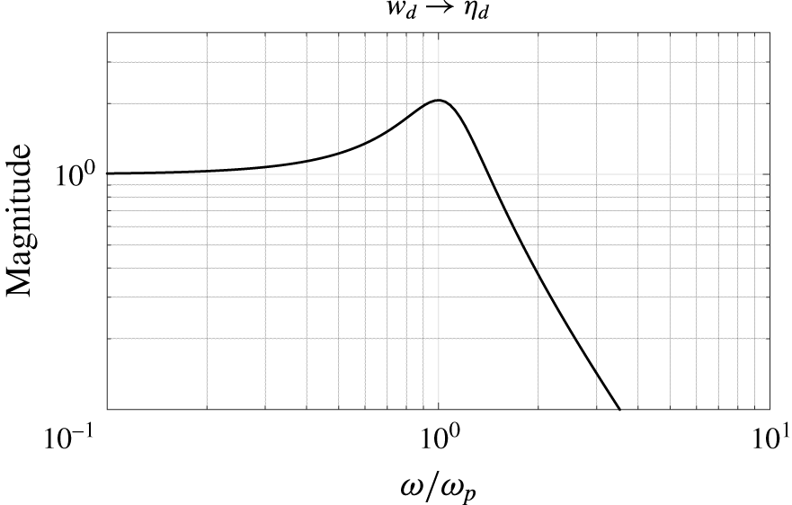
The low-pass filter (2.12) allows the frequency response shaping of
 $\boldsymbol{u}_{d}$
at the inflow. The parameters are chosen such that the filter amplifies the frequencies near the frequency
 $\unicode[STIX]{x1D714}$
of the perturbation mode. The damping ratio is set to
 $\unicode[STIX]{x1D701}=0.25$
. The natural frequency is chosen such that the peak frequency
 $\unicode[STIX]{x1D714}_{p}=\unicode[STIX]{x1D714}_{n}\sqrt{1-2\unicode[STIX]{x1D701}^{2}}$
, where the filter has the maximum magnitude, is equal to the frequency of the perturbation mode. The magnitude plot of the filter as a function of the normalised frequency
 $\unicode[STIX]{x1D714}/\unicode[STIX]{x1D714}_{p}$
is shown in figure 2. With these settings the filter amplifies the disturbance magnitude by approximately a factor two at
 $\unicode[STIX]{x1D714}_{p}$
. By increasing the magnitude at the perturbation frequency the controller will be better able to target the mode. The filter attenuates the disturbance at higher frequencies which will also make the controller design more robust to unresolved dynamics (Jones et al.
Reference Jones, Heins, Kerrigan, Morrison and Sharma2015). Finite-dimensional representations of the system (discussed in the next section) are used for the control design which only resolve a finite number of modes, typically those with a lower temporal frequency. By suppressing the magnitude of the disturbance at higher frequencies, the situation where the disturbance excites unresolved plant dynamics is avoided. This in turn avoids that the controller, which is designed based on the disturbance model, estimates unresolved plant dynamics. This phenomenon is also known as spillover and can destabilise the infinite-dimensional system (Balas Reference Balas1979).
Magnitude plot of the low-pass filter (2.12) used for the disturbance model. The frequency is normalised with the peak frequency
 $\unicode[STIX]{x1D714}_{p}$
.
The disturbance model defined by (2.11) and (2.12) can be written in state-space format as
 $$\begin{eqnarray}\displaystyle \left.\begin{array}{@{}c@{}}\left[\begin{array}{@{}c@{}}\dot{\unicode[STIX]{x1D702}}_{d}\\ \ddot{\unicode[STIX]{x1D702}}_{d}\end{array}\right]=\underbrace{\left[\begin{array}{@{}cc@{}}0 & 1\\ -\unicode[STIX]{x1D714}_{n}^{2} & -2\unicode[STIX]{x1D701}\unicode[STIX]{x1D714}_{n}\end{array}\right]}_{{\mathcal{A}}_{d}}\underbrace{\left[\begin{array}{@{}c@{}}\unicode[STIX]{x1D702}_{d}\\ \dot{\unicode[STIX]{x1D702}}_{d}\end{array}\right]}_{\bar{\boldsymbol{\unicode[STIX]{x1D702}}}_{d}}+\underbrace{\left[\begin{array}{@{}c@{}}0\\ \unicode[STIX]{x1D714}_{n}^{2}\end{array}\right]}_{{\mathcal{B}}_{d}}w_{d}\\ \boldsymbol{u}_{d}=\underbrace{\left[\begin{array}{@{}cc@{}}\tilde{\boldsymbol{u}}^{r} & -{\displaystyle \frac{1}{\unicode[STIX]{x1D714}}}\tilde{\boldsymbol{u}}^{i}\end{array}\right]}_{{\mathcal{C}}_{d}}\left[\begin{array}{@{}c@{}}\unicode[STIX]{x1D702}_{d}\\ \dot{\unicode[STIX]{x1D702}}_{d}\end{array}\right]\end{array}\right\}\Rightarrow \begin{array}{@{}l@{}}\dot{\bar{\boldsymbol{\unicode[STIX]{x1D702}}}}_{d}={\mathcal{A}}_{d}\bar{\boldsymbol{\unicode[STIX]{x1D702}}}_{d}+{\mathcal{B}}_{d}w_{d}\\ \boldsymbol{u}_{d}={\mathcal{C}}_{d}\bar{\boldsymbol{\unicode[STIX]{x1D702}}}_{d},\end{array} & & \displaystyle\end{eqnarray}$$
where
 $\bar{\boldsymbol{\unicode[STIX]{x1D702}}}_{d}=[\unicode[STIX]{x1D702}_{d},\dot{\unicode[STIX]{x1D702}}_{d}]$
is the state,
 $w_{d}$
is the external disturbance and the perturbation velocity
 $\boldsymbol{u}_{d}$
at the inflow is the output. For the case when multiple
 $N$
modes are accounted for in the control design, the state-space systems for the selected frequencies and wavenumbers can be combined in diagonal form as
 ${\mathcal{A}}_{d}=\text{diag}\{{\mathcal{A}}_{d_{1}},\ldots ,{\mathcal{A}}_{d_{N}}\}$
,
 ${\mathcal{B}}_{d}=\text{diag}\{{\mathcal{B}}_{d_{1}},\ldots ,{\mathcal{B}}_{d_{N}}\}$
and
 ${\mathcal{C}}_{d}=[{\mathcal{C}}_{d_{1}},\ldots ,{\mathcal{C}}_{d_{N}}]$
.
2.3.2 Selection of the perturbation modes
The next step is to select the modes that contribute to the transition process to include in the disturbance model (2.14) for control design. The modes are computed from the Orr–Sommerfeld equation. Let
 $\tilde{\boldsymbol{u}}=[\unicode[STIX]{x2202}\tilde{\unicode[STIX]{x1D713}}/\unicode[STIX]{x2202}y,-\unicode[STIX]{x2202}\tilde{\unicode[STIX]{x1D713}}/\unicode[STIX]{x2202}x]=[\tilde{\unicode[STIX]{x1D713}}^{\prime },-\text{i}\unicode[STIX]{x1D6FC}\tilde{\unicode[STIX]{x1D713}}]^{\text{T}}$
. The eigenfunction for the streamfunction
 $\tilde{\unicode[STIX]{x1D713}}$
satisfies the Orr–Sommerfeld equation
 $$\begin{eqnarray}\displaystyle \left.\begin{array}{@{}c@{}}\displaystyle \left(U-\frac{\unicode[STIX]{x1D714}}{\unicode[STIX]{x1D6FC}}\right)(\tilde{\unicode[STIX]{x1D713}}^{\prime \prime }-\unicode[STIX]{x1D6FC}^{2}\tilde{\unicode[STIX]{x1D713}})-U^{\prime \prime }\tilde{\unicode[STIX]{x1D713}}=-\frac{\text{i}}{\unicode[STIX]{x1D6FC}Re}(\tilde{\unicode[STIX]{x1D713}}^{\prime \prime \prime \prime }-2\unicode[STIX]{x1D6FC}^{2}\tilde{\unicode[STIX]{x1D713}}^{\prime \prime }+\unicode[STIX]{x1D6FC}^{4}\tilde{\unicode[STIX]{x1D713}}),\\ \tilde{\unicode[STIX]{x1D713}}(\pm 1)=\tilde{\unicode[STIX]{x1D713}}^{\prime }(\pm 1)=0,\end{array}\right\} & & \displaystyle\end{eqnarray}$$
which is an eigenvalue problem with
 $\tilde{\unicode[STIX]{x1D713}}$
the eigenfunction of the problem and with either
 $\unicode[STIX]{x1D6FC}$
or
 $\unicode[STIX]{x1D714}$
the eigenvalue of the problem. The prime superscript in (2.15) denotes differentiation with respect to
 $y$
. The spatial amplification theory is considered to generate the modes. Thus a real frequency
 $\unicode[STIX]{x1D714}$
is chosen and (2.15) is solved for the complex eigenfunction and complex wavenumber
 $\unicode[STIX]{x1D6FC}$
. At each frequency and Reynolds number this gives a spectrum of spatial eigenvalues. Figure 3 shows the spectrum at the most dominant frequency that includes the mode with the maximum growth rate given by the imaginary part of the spatial eigenvalue (wavenumber). For the case
 $Re=7000$
the dominant frequency is approximately
 $\unicode[STIX]{x1D714}=0.253$
. Only the least stable eigenvalues that contribute to a physical downstream response are shown in figure 3 (Schmid & Henningson Reference Schmid and Henningson2001, p. 260). The spectrum contains one spatially growing mode (
 $k=1$
) with a negative imaginary part. This is the leading or most unstable mode that contributes to the primary route to transition (Saric, Reed & Kerschen Reference Saric, Reed and Kerschen2002) in 2-D channel flows. The left branch
 $k=2,\ldots ,k=13,k=15$
are ‘centre modes’ (Kim & Bewley Reference Kim and Bewley2007) with very little support near the walls and represent perturbations in the free stream. Mode
 $k=14$
is highly stable and has negligible influence in the transition process. Figure 4 shows the spatial eigenvalue of the first or most unstable (
 $k=1$
) mode as a function of the temporal frequency. Although the flow is unstable over the frequency range
 $0.216\leqslant \unicode[STIX]{x1D714}\leqslant 0.286$
, only the leading mode calculated at the most amplified frequency
 $\unicode[STIX]{x1D714}=0.253$
is included in the control design. This will be referred to as the design point in the remainder of the paper. Figure 5 shows the shape of the eigenfunction for this particular mode. This mode is used to define the inflow perturbation (2.14). Note that the design frequency becomes part of the disturbance model. This model can easily be extended to include the dominant modes calculated for different temporal frequencies. However, it is found that adding more eigensolutions does not improve the performance of the control system. This is a direct result of the near-linear dependence of the leading eigenmodes for different temporal frequencies. In other words the modes are very similar. It will be shown in § 3 that also at other frequencies than the design point, the single mode inflow disturbance will quickly develop in-domain to a travelling wave with a spatial growth as predicted by the Orr–Sommerfeld equation (2.15).
Spatial Orr–Sommerfeld spectrum for
 $\unicode[STIX]{x1D714}=0.253$
and
 $Re=7000$
. Only the dominant eigenvalues that contribute to a physical downstream response are shown.

The leading or most unstable wavenumber as function of the temporal frequency
 $\unicode[STIX]{x1D714}$
at
 $Re=7000$
. (a) The imaginary part
 $\unicode[STIX]{x1D6FC}_{i}$
. Negative values of
 $\unicode[STIX]{x1D6FC}_{i}$
characterise unstable modes (grey region). (b) The real part
 $\unicode[STIX]{x1D6FC}_{r}$
. The point marked by ‘o’ corresponds to the most amplified frequency for the investigated conditions.

The selected eigenfunction included in the inflow disturbance model for the control design. The Orr–Sommerfeld eigenfunction for
 $u$
(a) and
 $v$
(b) calculated at
 $Re=7000$
,
 $\unicode[STIX]{x1D714}=0.253$
. The corresponding wavenumber for this mode is
 $\unicode[STIX]{x1D6FC}=1-0.0047i$
.

2.4 State-space formulation
In this section the linearised Navier–Stokes equations (LNSE) including the inputs, outputs and the inflow disturbance model are written as a boundary control system in the standard state-space format (
 $\dot{\boldsymbol{u}}={\mathcal{A}}\boldsymbol{u}+{\mathcal{B}}\unicode[STIX]{x1D753}$
,
 $\unicode[STIX]{x1D742}={\mathcal{C}}\boldsymbol{u}$
). This is required for defining the control objective and applying control theoretic tools. Boundary control systems do not fit directly into the standard form. However, we can extract the boundary controlled part of the dynamical model and rewrite the system on an extended state space in standard form. This method originates from Fattorini (Reference Fattorini1968) and has been applied for boundary control of wall-bounded shear flows (Högberg & Henningson Reference Högberg and Henningson2002; Högberg et al.
Reference Högberg, Bewley and Henningson2003a
; Chevalier et al.
Reference Chevalier, Hœpffner, Åkervik and Henningson2007). We also refer to Curtain & Zwart (Reference Curtain and Zwart1995, § 3.3) for more information on this formulation. Let
 ${\mathcal{X}}(\unicode[STIX]{x1D6FA})$
be the space of
 $n$
-dimensional divergence free functions defined on
 $\unicode[STIX]{x1D6FA}$
with inner product
 $(\boldsymbol{u}_{1},\boldsymbol{u}_{2})=\int _{\unicode[STIX]{x1D6FA}}\boldsymbol{u}_{1}\boldsymbol{\cdot }\boldsymbol{u}_{2}\,\text{d}\boldsymbol{x}$
and norm
 $\Vert \boldsymbol{u}_{1}\Vert _{2}=(\boldsymbol{u}_{1},\boldsymbol{u}_{1})^{1/2}$
where
 $\boldsymbol{u}_{1},\boldsymbol{u}_{2}\in {\mathcal{X}}$
. Furthermore, let the trajectory segment
 $\boldsymbol{u}(\cdot ,t)=\{\boldsymbol{u}(\boldsymbol{x},t),\boldsymbol{x}\in \unicode[STIX]{x1D6FA}\}$
be the state and
 $\boldsymbol{u}(t)|_{\unicode[STIX]{x1D6E4}}\in {\mathcal{U}}$
the value of
 $\boldsymbol{u}(t)$
on the boundary defined in a separable Hilbert space
 ${\mathcal{U}}$
. The LNSE (2.1) in
 ${\mathcal{X}}(\unicode[STIX]{x1D6FA})$
, including the boundary inputs (2.2), the measurements (2.5) and the controlled output (2.7), can be written as
 $$\begin{eqnarray}\displaystyle & \left.\begin{array}{@{}c@{}}\dot{\boldsymbol{u}}=\mathscr{A}\boldsymbol{u},\\ \mathscr{B}\boldsymbol{u}=\boldsymbol{u}_{c}+\boldsymbol{u}_{d},\\ \boldsymbol{ q}={\mathcal{Q}}\boldsymbol{ u},\\ \unicode[STIX]{x1D742}_{m}={\mathcal{C}}\boldsymbol{u}+\boldsymbol{w}_{n}.\end{array}\right\} & \displaystyle\end{eqnarray}$$
The operator
 $\mathscr{A}:D(\mathscr{A})\subset {\mathcal{X}}\mapsto {\mathcal{X}}$
corresponds to evaluating the linear differential operator of the LNSE. The pressure can be eliminated from the equations by using a space of velocity fields which are divergence free (Bewley et al.
Reference Bewley, Temam and Ziane2000), which is also done here (see also appendix A for the variational formulation).
 $\mathscr{B}:{\mathcal{X}}\mapsto {\mathcal{U}}$
is a boundary operator which maps the flow field to its values on the boundary and
 ${\mathcal{C}}$
,
 ${\mathcal{Q}}$
are output operators, respectively defined as
 $$\begin{eqnarray}\displaystyle & \mathscr{B}\boldsymbol{u}=\boldsymbol{u}|_{\unicode[STIX]{x1D6E4}_{D}},\quad {\mathcal{C}}_{i}\boldsymbol{u}=(\unicode[STIX]{x1D6FF}(x-x_{m}),\boldsymbol{t}\boldsymbol{\cdot }(\boldsymbol{n}\boldsymbol{\cdot }\unicode[STIX]{x1D735})\boldsymbol{u}|_{\unicode[STIX]{x1D6E4}_{r_{i}}}),\quad {\mathcal{Q}}_{i}\boldsymbol{u}=(h(x),\boldsymbol{t}\boldsymbol{\cdot }(\boldsymbol{n}\boldsymbol{\cdot }\unicode[STIX]{x1D735})\boldsymbol{u}|_{\unicode[STIX]{x1D6E4}_{r_{i}}}). & \displaystyle \nonumber\\ \displaystyle & & \displaystyle\end{eqnarray}$$
To extract the boundary controlled part the first step is to construct two operators
 ${\mathcal{Z}}_{c}$
,
 ${\mathcal{Z}}_{d}$
such that
 $$\begin{eqnarray}\displaystyle & \left.\begin{array}{@{}c@{}}{\mathcal{Z}}_{c\!}:{\mathcal{U}}\mapsto {\mathcal{X}},\quad \mathscr{B}{\mathcal{Z}}_{c}\boldsymbol{u}_{c}=\boldsymbol{u}_{c},\\ {\mathcal{Z}}_{d}:{\mathcal{U}}\mapsto {\mathcal{X}},\quad \mathscr{B}{\mathcal{Z}}_{d}\boldsymbol{u}_{d}=\boldsymbol{u}_{d}.\end{array}\right\} & \displaystyle\end{eqnarray}$$
The boundary condition can then be removed by decomposing the state into
 $$\begin{eqnarray}\boldsymbol{u}=\boldsymbol{u}_{h}+{\mathcal{Z}}_{c}\boldsymbol{u}_{c}+{\mathcal{Z}}_{d}\boldsymbol{u}_{d}.\end{eqnarray}$$
The dynamics of the new state
 $\boldsymbol{u}_{h}$
is governed by the following evolution equation with homogeneous boundary conditions (Curtain & Zwart Reference Curtain and Zwart1995)
 $$\begin{eqnarray}\displaystyle & \dot{\boldsymbol{u}}_{h}={\mathcal{A}}\boldsymbol{u}_{h}-{\mathcal{Z}}_{c}\dot{\boldsymbol{u}}_{c}+\mathscr{A}{\mathcal{Z}}_{c}\boldsymbol{u}_{c}-{\mathcal{Z}}_{d}\dot{\boldsymbol{u}}_{d}+\mathscr{A}{\mathcal{Z}}_{d}\boldsymbol{u}_{d}, & \displaystyle\end{eqnarray}$$
where the operator
 ${\mathcal{A}}:D({\mathcal{A}})\mapsto {\mathcal{X}}$
is defined as
 $$\begin{eqnarray}\displaystyle & \left.\begin{array}{@{}c@{}}{\mathcal{A}}\boldsymbol{u}_{h}(t)=\mathscr{A}\boldsymbol{u}_{h}(t),\quad \text{for}~\boldsymbol{u}_{h}\in D({\mathcal{A}}),\\ D({\mathcal{A}})=D(\mathscr{A})\cap \text{ker}(\mathscr{B})=\{\boldsymbol{u}_{h}\in {\mathcal{X}}|\boldsymbol{u}_{h}(t)|_{\unicode[STIX]{x1D6E4}_{D}}=0\}.\end{array}\right\} & \displaystyle\end{eqnarray}$$
If
 $\boldsymbol{u}_{h}$
is a solution of the homogeneous system (2.20), then
 $\boldsymbol{u}$
defined by (2.19) is a solution of the original system (2.16) (Fattorini Reference Fattorini1968; Curtain & Zwart Reference Curtain and Zwart1995). Equation (2.20) contains both the temporal inputs and their time derivatives which is undesirable since they are not independent inputs. This can be eliminated by reformulating (2.20) on the extended state space
 ${\mathcal{X}}^{e}={\mathcal{X}}\oplus {\mathcal{U}}$
 $$\begin{eqnarray}\displaystyle \left[\begin{array}{@{}c@{}}\dot{\boldsymbol{u}}_{h}\\ \dot{\boldsymbol{u}}_{c}\\ \dot{\boldsymbol{u}}_{d}\end{array}\right]=\left[\begin{array}{@{}ccc@{}}{\mathcal{A}} & \mathscr{A}{\mathcal{Z}}_{c} & \mathscr{A}{\mathcal{Z}}_{d}\\ 0 & 0 & 0\\ 0 & 0 & 0\end{array}\right]\left[\begin{array}{@{}c@{}}\boldsymbol{u}_{h}\\ \boldsymbol{u}_{c}\\ \boldsymbol{u}_{d}\end{array}\right]+\left[\begin{array}{@{}c@{}}-{\mathcal{Z}}_{c}\\ I\\ 0\end{array}\right]\dot{\boldsymbol{u}}_{c}+\left[\begin{array}{@{}c@{}}-{\mathcal{Z}}_{d}\\ 0\\ I\end{array}\right]\dot{\boldsymbol{u}}_{d}. & & \displaystyle\end{eqnarray}$$
The inflow perturbation velocity and the wall actuation velocity have become a state of the system in this formulation. The external input is actually the time derivative of the boundary velocity. From the actuator model (2.3) it follows that
 $\boldsymbol{u}_{c}={\mathcal{C}}_{c}\boldsymbol{\unicode[STIX]{x1D702}}_{c}$
,
 $\dot{\boldsymbol{u}}_{c}={\mathcal{C}}_{c}{\mathcal{A}}_{c}\boldsymbol{\unicode[STIX]{x1D702}}_{c}+{\mathcal{C}}_{c}{\mathcal{B}}_{c}\unicode[STIX]{x1D753}$
and from the disturbance model (2.14) it follows that
 $\boldsymbol{u}_{d}={\mathcal{C}}_{d}\boldsymbol{\unicode[STIX]{x1D702}}_{d}$
,
 $\dot{\boldsymbol{u}}_{d}={\mathcal{C}}_{d}{\mathcal{A}}_{d}\bar{\boldsymbol{\unicode[STIX]{x1D702}}}_{d}+{\mathcal{C}}_{d}{\mathcal{B}}_{d}w_{d}$
. Substituting these expressions in (2.22), and combining this system with the actuator dynamics (2.3) and the disturbance dynamics (2.14), gives the following augmented system
 $$\begin{eqnarray}\displaystyle & \left.\begin{array}{@{}c@{}}\begin{array}{@{}rcl@{}}\left[\begin{array}{@{}c@{}}\dot{\boldsymbol{u}}_{h}\\ \dot{\boldsymbol{\unicode[STIX]{x1D702}}}_{c}\\ \dot{\bar{\boldsymbol{\unicode[STIX]{x1D702}}}}_{d}\end{array}\right]\ & =\ & \underbrace{\left[\begin{array}{@{}ccc@{}}{\mathcal{A}} & \mathscr{A}{\mathcal{Z}}_{c}{\mathcal{C}}_{c}-{\mathcal{Z}}_{c}{\mathcal{C}}_{c}{\mathcal{A}}_{c} & \mathscr{A}{\mathcal{Z}}_{d}{\mathcal{C}}_{d}-{\mathcal{Z}}_{d}{\mathcal{C}}_{d}{\mathcal{A}}_{d}\\ 0 & {\mathcal{A}}_{c} & 0\\ 0 & 0 & {\mathcal{A}}_{d}\end{array}\right]}_{\bar{{\mathcal{A}}}}\underbrace{\left[\begin{array}{@{}c@{}}\boldsymbol{u}_{h}\\ \boldsymbol{\unicode[STIX]{x1D702}}_{c}\\ \bar{\boldsymbol{\unicode[STIX]{x1D702}}}_{d}\end{array}\right]}_{\boldsymbol{u}^{e}}\\ \ & \ & +\,\underbrace{\left[\begin{array}{@{}c@{}}-{\mathcal{Z}}_{c}{\mathcal{C}}_{c}{\mathcal{B}}_{c}\\ {\mathcal{B}}_{c}\\ 0\end{array}\right]}_{\bar{{\mathcal{B}}}_{c}}\unicode[STIX]{x1D753}+\underbrace{\left[\begin{array}{@{}c@{}}-{\mathcal{Z}}_{d}{\mathcal{C}}_{d}{\mathcal{B}}_{d}\\ 0\\ {\mathcal{B}}_{d}\end{array}\right]}_{\bar{{\mathcal{B}}}_{d}}w_{d},\end{array}\\ \boldsymbol{q}=\underbrace{\left[\begin{array}{@{}ccc@{}}{\mathcal{Q}} & {\mathcal{Q}}{\mathcal{Z}}_{c}{\mathcal{C}}_{c} & {\mathcal{Q}}{\mathcal{Z}}_{d}{\mathcal{C}}_{d}\end{array}\right]}_{\bar{{\mathcal{Q}}}}\left[\begin{array}{@{}c@{}}\boldsymbol{u}_{h}\\ \boldsymbol{\unicode[STIX]{x1D702}}_{c}\\ \bar{\boldsymbol{\unicode[STIX]{x1D702}}}_{d}\end{array}\right],\\ \unicode[STIX]{x1D742}_{m}=\underbrace{\left[\begin{array}{@{}ccc@{}}{\mathcal{C}} & {\mathcal{C}}{\mathcal{Z}}_{c}{\mathcal{C}}_{c} & {\mathcal{C}}{\mathcal{Z}}_{d}{\mathcal{C}}_{d}\end{array}\right]}_{\bar{{\mathcal{C}}}}\left[\begin{array}{@{}c@{}}\boldsymbol{u}_{h}\\ \boldsymbol{\unicode[STIX]{x1D702}}_{c}\\ \bar{\boldsymbol{\unicode[STIX]{x1D702}}}_{d}\end{array}\right]+\boldsymbol{w}_{n},\end{array}\right\} & \displaystyle\end{eqnarray}$$
where also included are the resulting output equations from the state transformation (2.19). Equation (2.23) can be compactly written as
 $$\begin{eqnarray}\displaystyle & \left.\begin{array}{@{}c@{}}\dot{\boldsymbol{u}}^{e}=\bar{{\mathcal{A}}}\boldsymbol{u}^{e}+\bar{{\mathcal{B}}}_{c}\unicode[STIX]{x1D753}+\bar{{\mathcal{B}}}_{d}w_{d},\\ \boldsymbol{q}=\bar{{\mathcal{Q}}}\boldsymbol{u}^{e},\\ \unicode[STIX]{x1D742}_{m}=\bar{{\mathcal{C}}}\boldsymbol{u}^{e}+\boldsymbol{w}_{n},\end{array}\right\} & \displaystyle\end{eqnarray}$$
with
 $\boldsymbol{u}^{e}$
the extended state. A final remark is given about the controllability of the system. By formulating the system on the extended state space (2.20) pure integrators have been added at the system external inputs. This results in additional system poles at the origin. As a result, the system in the form (2.20) is not stabilisable, which means that not all uncontrollable modes are asymptotically stable. This is a direct result of the fact that both the control and disturbance are defined at the boundary and both appear as a state in the system. It is not possible to influence the additional poles of the disturbance dynamics by means of control and vice versa (assumption (i) is violated, and assumptions (iii) and (iv) are violated for
 $\unicode[STIX]{x1D714}=0$
, see appendix B). By including the actuator dynamics and disturbance dynamics, the uncontrollable poles at the origin are moved to the stable left half-plane to the location of the eigenvalues of
 ${\mathcal{A}}_{c}$
and
 ${\mathcal{A}}_{d}$
. The state-space formulation (2.23) is thus stabilisable which allows the synthesis of
 ${\mathcal{H}}_{2}$
optimal controllers.
2.5 Finite-dimensional system
Equation (2.24) represents the continuous formulation of the flow control problem. For simulation and control design a finite-dimensional representation of (2.24) is required. In Tol et al. (Reference Tol, de Visser and Kotsonis2016) a framework is presented for deriving state-space descriptions for a general class of linear parabolic PDEs to which standard control theoretic tools can be applied. This method is also used in this work and uses multivariate B-splines of arbitrary degree and smoothness defined on triangulations (Farin Reference Farin1986; de Boor Reference de Boor and Farin1987; Lai & Schumaker Reference Lai and Schumaker2007) to find matrix representations of all operators in (2.23). This method has the flexibility of the finite element method to use local refinements and to cope with irregular domains and the high approximation power of spectral methods. The triangulations used to construct the simulation model, and the model that is used as a starting point for model reduction and control design are shown in figure 6. The use of spline spaces provides a convenient way for stating the degree and smoothness of the spline model. In addition, the approximation properties of such spline spaces have been extensively studied in the literature (Lai & Schumaker Reference Lai and Schumaker2007). Let
 ${\mathcal{T}}$
be the triangulation of
 $\unicode[STIX]{x1D6FA}$
. The spline space is the space of all smooth piecewise polynomial functions of arbitrary degree
 $d$
and arbitrary smoothness
 $r$
over
 ${\mathcal{T}}$
with
 $0\leqslant r<d$
 $$\begin{eqnarray}S_{d}^{r}({\mathcal{T}}):=s\in C^{r}(\unicode[STIX]{x1D6FA}):s|_{t}\in {\mathcal{P}}_{d},\quad \forall t\in {\mathcal{T}}.\end{eqnarray}$$
With
 ${\mathcal{P}}_{d}$
the space of all polynomials of total degree
 $d$
and
 $t$
denotes a triangle. We construct a basis for the smooth divergence free spline subspace
 ${\mathcal{S}}$
such that
 ${\mathcal{S}}\subset {\mathcal{X}}$
in conjunction with a Galerkin scheme to obtain a finite-dimensional representation of the governing equations. The pressure is eliminated from the equations by using a space of velocity fields which are divergence free and a suitable choice of the variational formulation. This will also avoid singularities in the numerical method. The Galerkin-type variational formulation through which the spline approximation is determined and the corresponding numerical method are described in detail in appendix A.
Triangulations used for the simulation model and the model that is used for model reduction and control design. (a) Triangulation with 960 triangles used for the control model. (b) Triangulation with 1920 triangles used for the simulation model.
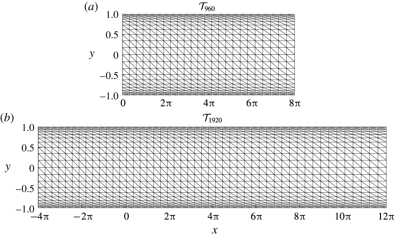
To derive the full-order control model a structured triangulation is used, refined near the walls to properly resolve the shear features of the flow consisting of
 $n_{t}=960$
triangles, and the
 ${\mathcal{S}}_{4}^{0}({\mathcal{T}}_{960})^{2}$
spline space is chosen as approximating space for the velocity field.
 $C^{0}$
continuous spline elements are chosen which allows an accurate interpolation of the actuator distribution function at the boundary. Degree
 $d=4$
elements are chosen which allows the construction of an exactly divergence free basis and to obtain better approximation properties (Awanou, Lai & Wenston Reference Awanou, Lai, Wenston, Chen and Lai2005; Lai & Schumaker Reference Lai and Schumaker2007). With this degree each element
 $t$
has a total of
 $N_{t}=15$
degrees of freedom. The complete basis for
 $L^{2}(\unicode[STIX]{x1D6FA})^{2}$
has a total of
 $N=n_{t}\times N_{t}\times 2=28\,800$
degrees of freedom. This basis is used to spatially discretise the system. The resulting discrete system is transformed to state-space format using a null-space projection method (Tol et al.
Reference Tol, de Visser and Kotsonis2016). This projection employs a similar state transformation as in (2.19), but in a discrete setting, and results in a reduced number of states that have a minimal non-zero support for the smooth divergence free spline space
 ${\mathcal{S}}\subset {\mathcal{X}}$
. The reduction is equal to the total rank
 $R^{\ast }$
of the discrete divergence, boundary and smoothness operators. The order of the state-space model resulting from the null-space projection is
 $N-R^{\ast }=5569$
. The large reduction can be contributed to the fact that the constrained smooth divergence free subspace is much smaller than the unconstrained space. The order of the model is sufficiently small to allow a direct application of balanced truncation for model reduction. For the case of spatially periodic boundary conditions the accuracy of the model can be assessed via comparison of the model spectra with the temporal spectra of the Orr–Sommerfeld equation (2.15). This comparison is demonstrated in § A.2. The numerical accuracy of the first 22 dominant eigenvalues varies between
 $2\times 10^{-8}\leqslant |\unicode[STIX]{x1D706}_{k}-\unicode[STIX]{x1D706}_{k}^{OS}|\leqslant 2\times 10^{-3}$
. This is considered accurate for the purpose of control design and demonstration. A more physical validation of the model for the non-periodic case considered in this study is conducted in § 3. A different model is used for simulating the response of system. The simulation model is defined on a longer domain with a total length of
 $L_{sim}=16\unicode[STIX]{x03C0}$
. A similar triangulation consisting of 1920 triangles is used and the simulation model has approximately the same accuracy as the control model. In the next sections we focus on the control model and use the notation (
 ${\mathcal{A}}$
,
 ${\mathcal{B}}$
,
 ${\mathcal{C}}$
,
 ${\mathcal{D}}$
) to represent the full-order finite-dimensional system and use the notation (
 $\unicode[STIX]{x1D63C}$
,
 $\unicode[STIX]{x1D63D}$
,
 $\unicode[STIX]{x1D63E}$
,
 $\unicode[STIX]{x1D63F}$
) to represent a reduced-order system resulting from balanced truncation.
2.6 Formulation of the
 ${\mathcal{H}}_{2}$
control problem

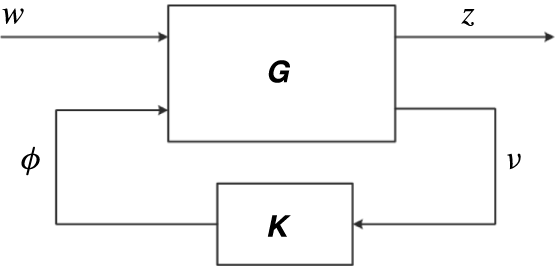
The general control configuration. System
 $\unicode[STIX]{x1D642}$
, controller
 $\unicode[STIX]{x1D646}$
, output measurement
 $\unicode[STIX]{x1D742}$
, control input
 $\unicode[STIX]{x1D753}$
, performance objective
 $\boldsymbol{z}$
and exogenous disturbances
 $\boldsymbol{w}$
.
In this section the feedback design problem for the state-space representation of the flow (2.24) is cast as an
 ${\mathcal{H}}_{2}$
optimisation problem. The state-space formulas for the optimal solution are given in appendix B. We refer to Doyle et al. (Reference Doyle, Glover, Khargonekar and Francis1989), Zhou et al. (Reference Zhou, Doyle and Glover1996), Skogestad & Postlethwaite (Reference Skogestad and Postlethwaite2005) for more detail on this control theory. The main objective of the feedback control design is to find a control input
 $\unicode[STIX]{x1D753}$
based on the output measurement
 $\unicode[STIX]{x1D742}_{m}$
that minimises the wall shear stress defined by
 $\boldsymbol{q}$
in the presence of the disturbances
 $w_{d}$
and
 $\boldsymbol{w}_{n}$
. First the standard control formulation that is considered by
 ${\mathcal{H}}_{2}$
control is presented. The application of
 ${\mathcal{H}}_{2}$
control to the state-space representation of the flow (2.24) will follow thereafter. Let
 $\boldsymbol{w}$
be the vector of exogenous disturbances and
 $\boldsymbol{z}$
the vector of performance measures to be minimised. The
 ${\mathcal{H}}_{2}$
control problem is a disturbance rejection problem and considers the standard control configuration shown in figure 7 which is described by
 $$\begin{eqnarray}\displaystyle & \left.\begin{array}{@{}c@{}}\left[\begin{array}{@{}c@{}}\boldsymbol{z}\\ \unicode[STIX]{x1D742}\end{array}\right]=\unicode[STIX]{x1D642}(s)\left[\begin{array}{@{}c@{}}\boldsymbol{w}\\ \unicode[STIX]{x1D753}\end{array}\right]=\left[\begin{array}{@{}cc@{}}\unicode[STIX]{x1D642}_{zw}(s) & \unicode[STIX]{x1D642}_{z\unicode[STIX]{x1D719}}(s)\\ \unicode[STIX]{x1D642}_{\unicode[STIX]{x1D708}w}(s) & \unicode[STIX]{x1D642}_{\unicode[STIX]{x1D708}\unicode[STIX]{x1D719}}(s)\end{array}\right]\left[\begin{array}{@{}c@{}}\boldsymbol{w}\\ \unicode[STIX]{x1D753}\end{array}\right],\\ \unicode[STIX]{x1D753}=\unicode[STIX]{x1D646}(s)\unicode[STIX]{x1D742},\end{array}\right\} & \displaystyle\end{eqnarray}$$
with
 $\unicode[STIX]{x1D646}(s)$
the controller to be synthesised and
 $\unicode[STIX]{x1D642}(s)$
the open-loop transfer function matrix of the generalised plant defined by
 $$\begin{eqnarray}\unicode[STIX]{x1D642}(s)={\mathcal{C}}_{p}(sI-{\mathcal{A}}_{p})^{-1}{\mathcal{B}}_{p}+{\mathcal{D}}_{p},\end{eqnarray}$$
with the state-space realisation

To account for the state disturbances
 $w_{d}$
and the measurement noise
 $\boldsymbol{w}_{n}$
in a
 ${\mathcal{H}}_{2}$
control framework the state-space system (2.24) is formulated as a generalised plant (2.28) and scaled in terms of two parameters which may be individually adjusted to achieve the desired closed-loop performance. A similar scaling was also presented in Bewley & Liu (Reference Bewley and Liu1998). The control objective is to counteract the influence of the state disturbance
 $w_{d}$
on the controlled output defined by
 $\boldsymbol{q}=\bar{{\mathcal{Q}}}\boldsymbol{u}^{e}$
. Therefore the controlled output is used to define the performance measure
 $\boldsymbol{z}$
 $$\begin{eqnarray}\boldsymbol{z}=\left[\begin{array}{@{}c@{}}\bar{{\mathcal{Q}}}\\ 0\end{array}\right]\boldsymbol{u}^{e}+\left[\begin{array}{@{}c@{}}0\\ lI\end{array}\right]\unicode[STIX]{x1D753},\end{eqnarray}$$
which also includes a penalty on the control defined by the parameter
 $l$
. The parameter
 $l$
determines the trade-off between a low control effort (
 $\unicode[STIX]{x1D753}^{\text{T}}\unicode[STIX]{x1D753}$
) and a low controlled output energy (
 $\boldsymbol{q}^{\text{T}}\boldsymbol{q}$
). For the design of the controller, decisions must be made about the expected state disturbances and measurement noise. The temporal magnitude of these disturbances in the state-space system is defined by the expected covariances of the temporal state disturbance (2.13) and the measurement noise (2.6). In this study it is assumed that nothing is known a priori about the expected covariances. To make a parametric study for the controller design tractable, a relative magnitude of the measurement noise is defined
 $$\begin{eqnarray}\unicode[STIX]{x1D6FE}=\frac{\unicode[STIX]{x1D70E}_{n}}{\unicode[STIX]{x1D70E}_{d}},\end{eqnarray}$$
which is the ratio between the root mean square of the expected variance of respectively the sensor noise and the state disturbance. The state disturbance and measurement noise are respectively modelled as
 $w_{d}=\unicode[STIX]{x1D70E}_{d}w_{1}$
and
 $\boldsymbol{w}_{n}=\unicode[STIX]{x1D70E}_{n}\boldsymbol{w}_{2}$
with
 $w_{1}$
and
 $\boldsymbol{w}_{2}$
defined as white noise with unit intensity. The system is parameterised in terms of
 $\unicode[STIX]{x1D6FE}$
by defining a new scaled observation that is used for feedback
 $$\begin{eqnarray}\displaystyle \unicode[STIX]{x1D742}=\frac{\unicode[STIX]{x1D6FE}}{\unicode[STIX]{x1D70E}_{n}}\unicode[STIX]{x1D742}_{m} & = & \displaystyle \frac{\unicode[STIX]{x1D6FE}}{\unicode[STIX]{x1D70E}_{n}}(\bar{{\mathcal{C}}}\boldsymbol{u}^{e}+\unicode[STIX]{x1D70E}_{n}\boldsymbol{w}_{2})\nonumber\\ \displaystyle & = & \displaystyle \frac{\unicode[STIX]{x1D6FE}}{\unicode[STIX]{x1D70E}_{n}}\bar{{\mathcal{C}}}\boldsymbol{u}^{e}+\unicode[STIX]{x1D6FE}\boldsymbol{w}_{2}\end{eqnarray}$$
and the system is normalised such that
 $\unicode[STIX]{x1D70E}_{d}=1$
. Using this normalisation it follows from (2.30) that
 $\unicode[STIX]{x1D6FE}=\unicode[STIX]{x1D70E}_{n}$
and the observation (2.31) is obtained by a simple change of variables. For the control design
 $\unicode[STIX]{x1D6FE}$
does not represent a physical root mean square value of the measurement noise, but a relative measure with respect to the state disturbance, used to tune the controller. Defining the vector of disturbances as
 $\boldsymbol{w}=[w_{1},~\boldsymbol{w}_{2}^{\text{T}}]^{\text{T}}$
and the following system matrices
 $$\begin{eqnarray}\displaystyle & \left.\begin{array}{@{}c@{}}{\mathcal{A}}_{p}=\bar{{\mathcal{A}}},\quad {\mathcal{B}}_{1}=\left[\begin{array}{@{}cc@{}}\unicode[STIX]{x1D70E}_{d}\bar{{\mathcal{B}}}_{d} & 0\end{array}\right],\quad {\mathcal{B}}_{2}=\bar{{\mathcal{B}}}_{c},\\ {\mathcal{C}}_{1}=\left[\begin{array}{@{}c@{}}\bar{{\mathcal{Q}}}\\ 0\end{array}\right],\quad {\mathcal{D}}_{12}=\left[\begin{array}{@{}c@{}}0\\ lI\end{array}\right],\quad {\mathcal{C}}_{2}={\displaystyle \frac{\unicode[STIX]{x1D6FE}}{\unicode[STIX]{x1D70E}_{n}}}\bar{{\mathcal{C}}},\quad {\mathcal{D}}_{21}=\left[\begin{array}{@{}cc@{}}0 & \unicode[STIX]{x1D6FE}I\end{array}\right],\end{array}\right\} & \displaystyle\end{eqnarray}$$
the system (2.24) can be written as a generalised plant with the state-space formulation (2.28), that is
 $$\begin{eqnarray}\displaystyle \left.\begin{array}{@{}c@{}}\dot{\boldsymbol{u}^{e}}={\mathcal{A}}_{p}\boldsymbol{u}^{e}+{\mathcal{B}}_{1}\boldsymbol{w}+{\mathcal{B}}_{2}\unicode[STIX]{x1D753},\\ \boldsymbol{z}={\mathcal{C}}_{1}\boldsymbol{u}^{e}+{\mathcal{D}}_{12}\unicode[STIX]{x1D753},\\ \unicode[STIX]{x1D742}={\mathcal{C}}_{2}\boldsymbol{u}^{e}+{\mathcal{D}}_{21}\boldsymbol{w}.\end{array}\right\} & & \displaystyle\end{eqnarray}$$
The
 ${\mathcal{H}}_{2}$
control design problem for this system is to find a controller
 $\unicode[STIX]{x1D646}(s)$
that, based on the measurement information
 $\unicode[STIX]{x1D742}$
, generates a control input
 $\unicode[STIX]{x1D753}$
which stabilises the system (2.33) internally and minimises
 $$\begin{eqnarray}\Vert \unicode[STIX]{x1D64F}_{zw}(s)\Vert _{2}=\sqrt{\frac{1}{2\unicode[STIX]{x03C0}}\int _{-\infty }^{\infty }\text{Trace}\{\unicode[STIX]{x1D64F}_{zw}^{\ast }(\text{i}\unicode[STIX]{x1D714})\unicode[STIX]{x1D64F}_{zw}(\text{i}\unicode[STIX]{x1D714})\}\,\text{d}\unicode[STIX]{x1D714}}=\sqrt{\frac{1}{2\unicode[STIX]{x03C0}}\int _{-\infty }^{\infty }\mathop{\sum }_{i,j}|\unicode[STIX]{x1D61B}_{zw}^{i,j}(\text{i}\unicode[STIX]{x1D714})|^{2}\,\text{d}\unicode[STIX]{x1D714}}.\end{eqnarray}$$
Equation (2.34) is referred to as the
 ${\mathcal{H}}_{2}$
-norm of the closed-loop transfer function matrix
 $\unicode[STIX]{x1D64F}_{zw}$
from the external disturbances
 $\boldsymbol{w}$
to the control objectives
 $\boldsymbol{z}$
and
 $|\unicode[STIX]{x1D61B}_{zw}^{i,j}|$
denotes the magnitude of the closed-loop transfer function from the
 $j$
th disturbance to the
 $i$
th objective.
 $\unicode[STIX]{x1D64F}_{zw}$
is given by
 $$\begin{eqnarray}\unicode[STIX]{x1D64F}_{zw}(s)=\frac{\boldsymbol{z}(s)}{\boldsymbol{w}(s)}=\unicode[STIX]{x1D642}_{zw}(s)+\unicode[STIX]{x1D642}_{z\unicode[STIX]{x1D719}}(s)\unicode[STIX]{x1D646}(s)(I-\unicode[STIX]{x1D642}_{\unicode[STIX]{x1D708}\unicode[STIX]{x1D719}}(s)\unicode[STIX]{x1D646}(s))^{-1}\unicode[STIX]{x1D642}_{\unicode[STIX]{x1D708}w}(s),\end{eqnarray}$$
which follows from (2.26). Physically, the
 ${\mathcal{H}}_{2}$
norm in (2.34) can be interpreted as the amplification of the system from
 $\boldsymbol{w}$
to
 $\boldsymbol{z}$
integrated over all frequencies. In the time domain, this is equivalent to the variance amplification of stochastic disturbances (Jovanovic & Bamieh Reference Jovanovic and Bamieh2005). By minimising the
 ${\mathcal{H}}_{2}$
norm, the controlled output power
 $E[\boldsymbol{z}^{\text{T}}\boldsymbol{z}]$
of the system, due to unit white Gaussian disturbances
 $\boldsymbol{w}$
, is minimised. The state-space formulas for the optimal controller
 $\unicode[STIX]{x1D646}(s)$
that minimise (2.34) are given in appendix B. It combines a state estimator (Kalman filter) for the flow field and a state feedback, and has a state-space description of the form
 $$\begin{eqnarray}\displaystyle \left.\begin{array}{@{}c@{}}\dot{\boldsymbol{u}}_{K}^{e}={\mathcal{A}}_{K}\boldsymbol{u}_{K}^{e}+{\mathcal{B}}_{K}\unicode[STIX]{x1D742},\\ \unicode[STIX]{x1D753}={\mathcal{C}}_{K}\boldsymbol{u}_{K}^{e},\end{array}\right\} & & \displaystyle\end{eqnarray}$$
with
 $\boldsymbol{u}_{K}^{e}$
the estimated state and
 ${\mathcal{A}}_{K}={\mathcal{A}}+{\mathcal{B}}_{2}{\mathcal{C}}_{K}-{\mathcal{B}}_{K}{\mathcal{C}}_{2}$
. The controller input matrix
 ${\mathcal{B}}_{K}$
represents the estimator gain and the output matrix
 ${\mathcal{C}}_{K}$
represents the state feedback gain. The controller (2.36) can be structured using the separation principle, which means that the estimator and state feedback can be tuned independently. Thus the control penalty
 $l$
and the estimation parameter
 $\unicode[STIX]{x1D6FE}$
may be individually adjusted to achieve the desired characteristics for the closed-loop system
 $\unicode[STIX]{x1D64F}_{zw}$
. A low value for the control penalty
 $l$
results in higher gain state feedback
 ${\mathcal{C}}_{K}$
. Similarly, when
 $\unicode[STIX]{x1D6FE}$
is small (high signal to noise ratio) the observation is fed back more aggressively (high observer gain
 ${\mathcal{B}}_{K}$
) than when
 $\unicode[STIX]{x1D6FE}$
is high. The controller
 $\unicode[STIX]{x1D646}(s)$
in (2.36) represents the full-order controller. Such a high-order controller is usually not real time implementable for practical flow configurations. To synthesise a reduced-order controller
 $\unicode[STIX]{x1D646}_{r}(s)$
for the high-order plant the so-called reduce-then-design approach (Anderson & Liu Reference Anderson and Liu1989) is used, which is discussed in detail in the next section. This section also includes a parametric study for the parameters
 $\unicode[STIX]{x1D6FE}$
and
 $l$
.
3 Controller design and synthesis
In this section the reduced-order controller is designed and synthesised for the problem defined in the previous section. An input–output analysis (Bagheri et al. Reference Bagheri, Brandt and Henningson2009b ) is conducted in § 3.1 for the uncontrolled system using the spatio-temporal frequency response (Baramov et al. Reference Baramov, Tutty and Rogers2004; Jovanovic & Bamieh Reference Jovanovic and Bamieh2005) to identify the perturbation modes that are captured by the inflow disturbance model and are retained in the reduced-order model. The input–output analysis reveals the non-modal transients introduced by the inflow disturbance as well as the modal unstable perturbation modes. In § 3.2 a reduced-order model that captures the input–output behaviour is derived using balanced truncation. This model is used to design the optimal controller and the truncated dynamics is taken into account in the control system design. This section also includes a parametric study for the estimator and state feedback design problem. Finally, the closed-loop performance of three selected controllers is evaluated in the frequency domain in § 3.3. These three controllers will also be evaluated in § 4 using numerical simulations of the closed-loop system.
3.1 Analysis of the uncontrolled system
The magnitude of the spatio-temporal frequency response from the inflow disturbance
 $w_{1}$
to the shear along the lower wall
 $\unicode[STIX]{x1D708}_{1}(x,y=-1)$
. The 10 contour levels lie within
 $|G_{\unicode[STIX]{x1D708}_{1}w_{1}}|\in [6.9,~69.4]$
.
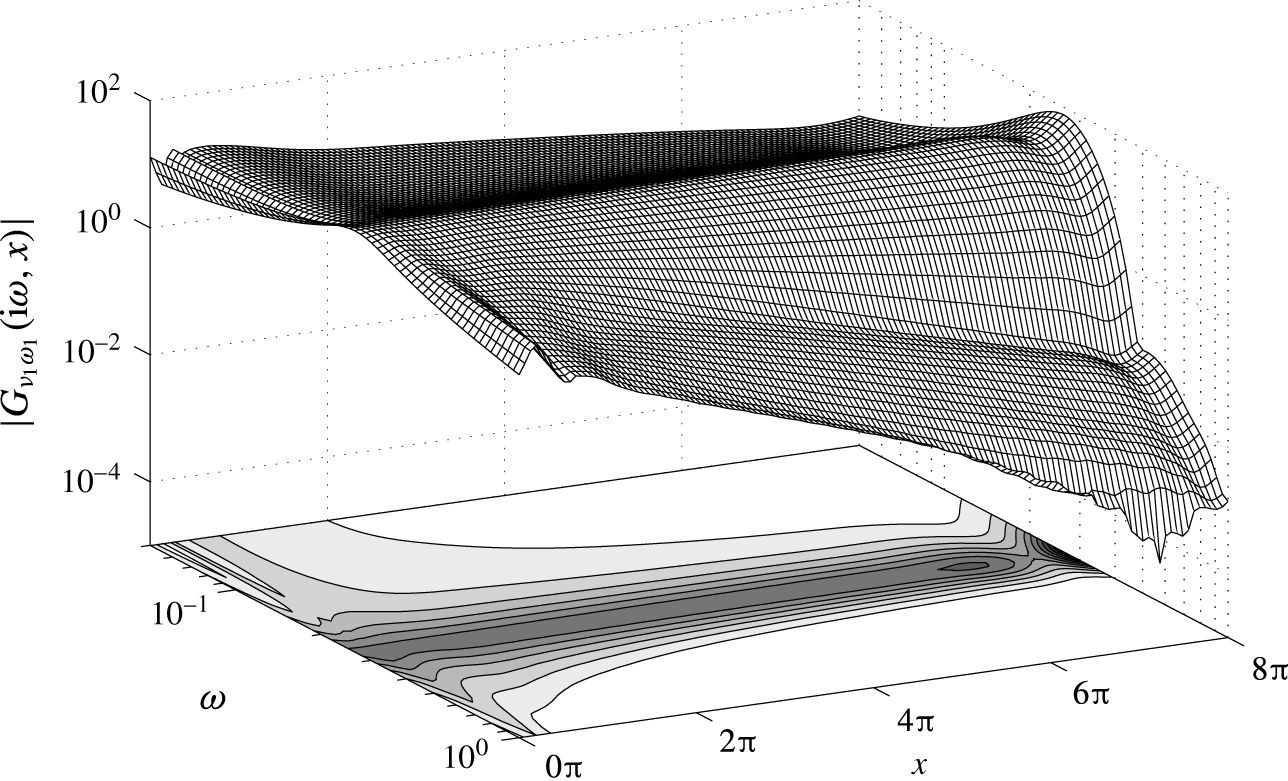
In this section the uncontrolled system from the disturbance input
 $\boldsymbol{w}$
to the shear output
 $\unicode[STIX]{x1D742}$
, that is
 $\unicode[STIX]{x1D642}_{\unicode[STIX]{x1D708}w}=[\unicode[STIX]{x1D642}_{\unicode[STIX]{x1D708}w_{1}},\unicode[STIX]{x1D642}_{\unicode[STIX]{x1D708}w_{2}}]$
in (2.26), is analysed in the frequency domain. In particular the effect of the inflow disturbance
 $w_{1}$
on
 $\unicode[STIX]{x1D742}$
is investigated from an input–output viewpoint. The disturbance input
 $w_{1}$
excites the Orr–Sommerfeld eigenfunction calculated for the most amplified frequency (
 $\unicode[STIX]{x1D714}=0.253$
) at the inflow, see also § 2.3 and figure 5. The perturbation shear stress created by the disturbance along the complete lower wall,
 $\unicode[STIX]{x1D708}_{1}(x)=(\unicode[STIX]{x2202}u/\unicode[STIX]{x2202}y)(x,-1)$
, is considered as output in the analysis. In this way the spatial transients created by the inflow disturbance can be evaluated and the perturbation modes that are excited can be identified. The same results hold for the upper wall due to the symmetry of the geometry. If a linear system is forced by a sinusoidal input at a particular frequency, once the initial temporal transients have died out asymptotically, the output will also be sinusoidal, at the same frequency, but with a change in amplitude and a phase shift. The magnitude amplification and phase shift of the output are equal to the magnitude and phase of the frequency response of the system. The frequency response is obtained by evaluating the transfer function on the imaginary axis, that is
 $s=\text{i}\unicode[STIX]{x1D714}$
. The asymptotic response for the shear output along the lower wall in the spatio-temporal frequency domain is given by
 $$\begin{eqnarray}\unicode[STIX]{x1D708}_{1}(\text{i}\unicode[STIX]{x1D714},x)=G_{\unicode[STIX]{x1D708}_{1}w_{1}}(\text{i}\unicode[STIX]{x1D714},x)w_{1}(\text{i}\unicode[STIX]{x1D714}),\end{eqnarray}$$
where
 $G_{\unicode[STIX]{x1D708}_{1}w_{1}}(\text{i}\unicode[STIX]{x1D714},x)$
is obtained from the
 $(1,1)$
element of
 $$\begin{eqnarray}\unicode[STIX]{x1D642}_{\unicode[STIX]{x1D708}w}(\text{i}\unicode[STIX]{x1D714},x)={\mathcal{C}}_{2}(x)(\text{i}\unicode[STIX]{x1D714}I-{\mathcal{A}}_{p})^{-1}{\mathcal{B}}_{1}.\end{eqnarray}$$
 $G_{\unicode[STIX]{x1D708}_{1}w_{1}}(\text{i}\unicode[STIX]{x1D714},x)$
is the spatio-temporal frequency response function (Jovanovic & Bamieh Reference Jovanovic and Bamieh2005) from the inflow disturbance
 $w_{1}$
to the shear stress along the lower wall. It is a function of temporal frequency and streamwise direction.
 $G_{\unicode[STIX]{x1D708}_{1}w_{1}}(\text{i}\unicode[STIX]{x1D714},x)$
is visualised using the magnitude bode plot
 $|G_{\unicode[STIX]{x1D708}_{1}w_{1}}(\text{i}\unicode[STIX]{x1D714},x)|$
which is shown in figure 8. To support the interpretation of the magnitude the fully developed open-loop response for
 $\unicode[STIX]{x1D714}=0.25$
and
 $\unicode[STIX]{x1D714}=0.35$
is shown in figure 9. The effect of the low-pass filter (2.12) on the magnitude at the inflow and the amplification at the design frequency
 $\unicode[STIX]{x1D714}=0.253$
can clearly be observed. After initial spatial transients near the inflow boundary, the modal perturbations are revealed and the magnitude linearly increases or decreases depending on the frequency of
 $w_{1}$
. At the design frequency an insignificant transient is involved for the mode to develop in the domain. Larger transients can be observed near the inflow at other frequencies than the design point. These non-modal transients do not cause a problem for control design as they have died out in the control region (
 $x>2\unicode[STIX]{x03C0}$
). The outflow boundary condition (2.1d
) gives rise to an artificial gain near the outflow
 $x>6\unicode[STIX]{x03C0}$
. This does not result in reflections (wiggles) in the control domain. No special attention needs to be taken for the non-physical region as long as no measurement sensors are placed in this region. For validation purposes the exponential growth for the perturbation shear output is compared with predictions from linear stability theory. The exponential growth can be calculated using
 $$\begin{eqnarray}\unicode[STIX]{x1D6FC}_{i}=-\frac{1}{x_{1}-x_{0}}\ln \frac{|G_{\unicode[STIX]{x1D708}_{1}w_{1}}(\text{i}\unicode[STIX]{x1D714},x_{1})|}{|G_{\unicode[STIX]{x1D708}_{1}w_{1}}(\text{i}\unicode[STIX]{x1D714},x_{0})|}.\end{eqnarray}$$
The location of the shear sensor
 $x_{0}=x_{m}=2.39\unicode[STIX]{x03C0}$
and the location of the controlled shear output
 $x_{1}=x_{q}=5.57\unicode[STIX]{x03C0}$
are chosen to compute the growth rate. Within this region the magnitude varies linearly over a wide range of frequencies. Figure 10 shows the magnitude of
 $G_{\unicode[STIX]{x1D708}_{1}w_{1}}(\text{i}\unicode[STIX]{x1D714},x)$
at the two spatial locations and the exponential growth rate of the magnitude compared with the growth rates from LST. Good agreement with LST predictions can be observed. Both the model and the OS equation predict instability within the range
 $0.216\leqslant \unicode[STIX]{x1D714}\leqslant 0.286$
. The real part of the wavenumber
 $\unicode[STIX]{x1D6FC}_{r}$
and the corresponding wavelength
 $\unicode[STIX]{x1D706}_{x}=2\unicode[STIX]{x03C0}/\unicode[STIX]{x1D6FC}_{r}$
of the perturbation can be evaluated using the phase response of the system. Let
 $\angle G_{\unicode[STIX]{x1D708}_{1}w_{1}}(\text{i}\unicode[STIX]{x1D714},x)$
be the phase in degrees for the shear output along the lower wall. The real part of the wavenumber can be calculated using
 $$\begin{eqnarray}\unicode[STIX]{x1D6FC}_{r}=\frac{|\angle G_{\unicode[STIX]{x1D708}_{1}w_{1}}(\text{i}\unicode[STIX]{x1D714},x_{1})-\angle G_{\unicode[STIX]{x1D708}_{1}w_{1}}(\text{i}\unicode[STIX]{x1D714},x_{0})|{\displaystyle \frac{\unicode[STIX]{x03C0}}{180}}}{x_{1}-x_{0}}.\end{eqnarray}$$
Figure 11 shows the phase at the two spatial locations and the resulting wavenumbers compared with the predictions from LST. It can be observed that also the wavelengths are in good agreement with LST. At
 $\unicode[STIX]{x1D714}=0.25$
LST predicts a wavelength of
 $\unicode[STIX]{x1D706}_{x}=2\unicode[STIX]{x03C0}/\unicode[STIX]{x1D6FC}_{r}\approx 2\unicode[STIX]{x03C0}$
and at
 $\unicode[STIX]{x1D714}=0.35$
a wavelength of
 $\unicode[STIX]{x1D706}_{x}\approx 1.6\unicode[STIX]{x03C0}$
. These wavelengths can also be observed in figure 9.
Fully developed open-loop response of the streamwise perturbation velocity for two inflow disturbance frequencies. (a) Shows 10 levels in the range
 $u\in [-1.61,1.61]$
. (b) Shows 10 levels in the range
 $u\in [-1.00,1.00]$
.

These results verify that the single mode inflow disturbance model accurately captures the wavelengths and growth rates in a wider frequency band in the actuator/sensor region. Also at other frequencies than the design frequency, the disturbance will quickly develop in-domain to a travelling wave with a spatial wavelength and growth rate as predicted by the Orr–Sommerfeld equation. It provides confidence that the followed modelling procedure allows for an efficient estimation of the dominant flow perturbations in the localised control domain using wall shear sensors. In the next section the controller is designed to reduce the magnitude of the shear downstream of the control actuators.
(a) Magnitude of the shear output at two
 $x$
-locations and (b) resulting exponential growth (3.3) compared with the solutions of the Orr–Sommerfeld equation.

(a) Phase of the shear output at two
 $x$
-locations and (b) resulting wavelength (3.4) compared with the solutions of the Orr–Sommerfeld equation.
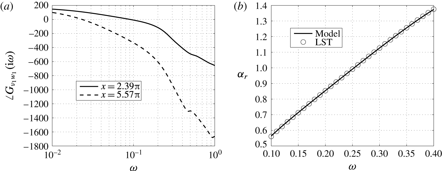
3.2 Reduced-order controller
The reduce-then-design approach (Anderson & Liu Reference Anderson and Liu1989) is used to construct a reduced-order controller for the high-order plant. First, exact balanced truncation (Moore Reference Moore1981) is applied to construct a reduced-order model of the full-order system after which the ROM is used to synthesise the optimal controller. Exact balanced truncation requires dense matrix factorisations and generally results in a computational complexity of
 $O(N^{3})$
and a storage requirement of
 $O(N^{2})$
. Exact balanced truncation is not computationally tractable for very large systems and approximate methods, such as proposed by Rowley (Reference Rowley2005), could be used in this case. However, the modelling approach in this paper avoids very large systems through localised computations allowing to apply exact balanced truncation (
 $N=5569$
for the control model). Since the current flow configuration is globally stable, balanced truncation can directly be applied without the need of separating the stable and unstable subspaces. Only the application of balanced truncation for model reduction and control design is discussed in this section. We refer to Moore (Reference Moore1981) for more detail and to Rowley (Reference Rowley2005), Kim & Bewley (Reference Kim and Bewley2007) for more background in the context of flow control.
Balanced truncation extracts the most controllable and observable modes of the system and first involves creating a balanced realisation of the system such that each state has an equal measure for both controllability and observability. Let
 $\unicode[STIX]{x1D642}_{b}(s)=({\mathcal{A}}_{b},{\mathcal{B}}_{b},{\mathcal{C}}_{b},{\mathcal{D}}_{b})$
be a balanced realisation of the generalised plant
 $\unicode[STIX]{x1D642}(s)=({\mathcal{A}}_{p},{\mathcal{B}}_{p},{\mathcal{C}}_{p},{\mathcal{D}}_{p})$
given by (2.28) such that the controllability Gramian and observability Gramian respectively defined as
 $$\begin{eqnarray}\displaystyle & \displaystyle \unicode[STIX]{x1D64B}=\int _{0}^{\infty }\text{e}^{{\mathcal{A}}_{b}t}{\mathcal{B}}_{b}{\mathcal{B}}_{b}^{T}\text{e}^{{\mathcal{A}}_{b}^{T}t}\,\text{d}t, & \displaystyle\end{eqnarray}$$
 $$\begin{eqnarray}\displaystyle & \displaystyle \unicode[STIX]{x1D64C}=\int _{0}^{\infty }\text{e}^{{\mathcal{A}}_{b}^{T}t}{\mathcal{C}}_{b}^{T}{\mathcal{C}}_{b}\text{e}^{{\mathcal{A}}_{b}t}\,\text{d}t & \displaystyle\end{eqnarray}$$
are given by
 $\unicode[STIX]{x1D64B}=\unicode[STIX]{x1D64C}=\text{diag}(\unicode[STIX]{x1D70E}_{1}^{H},\unicode[STIX]{x1D70E}_{2}^{H},\ldots ,\unicode[STIX]{x1D70E}_{N}^{H})=:\unicode[STIX]{x1D72E}$
where
 $\unicode[STIX]{x1D70E}_{1}^{H}\geqslant \unicode[STIX]{x1D70E}_{2}^{H}\geqslant \cdots \geqslant \unicode[STIX]{x1D70E}_{N}^{H}\geqslant 0$
are the Hankel singular values of the system. An efficient algorithm for creating balanced realisations is available in Matlab (balreal). This algorithm computes the similarity transformation
 $\boldsymbol{u}_{b}^{e}\mapsto \unicode[STIX]{x1D64E}\boldsymbol{u}^{e}$
, which balances the plant matrices through
 ${\mathcal{A}}_{b}=\unicode[STIX]{x1D64E}^{-1}{\mathcal{A}}_{p}\unicode[STIX]{x1D64E}$
,
 ${\mathcal{B}}_{b}=\unicode[STIX]{x1D64E}^{-1}{\mathcal{B}}_{p}$
,
 ${\mathcal{C}}_{b}={\mathcal{C}}_{p}\unicode[STIX]{x1D64E}$
and
 ${\mathcal{D}}_{b}={\mathcal{D}}_{p}$
. The similarity transformation
 $\unicode[STIX]{x1D64E}$
is obtained from the Cholesky factorisation of the Gramians (Laub et al.
Reference Laub, Heath, Paige and Ward1987). The Gramians are computed by solving a set of Lyapunov equations (Moore Reference Moore1981). This method is also stable if the system contains nearly uncontrollable/unobservable modes which are present in the linearised Navier–Stokes operator (Bewley & Liu Reference Bewley and Liu1998; Kim & Bewley Reference Kim and Bewley2007).
The balanced realisation and corresponding singular values can be partitioned as
 $$\begin{eqnarray}{\mathcal{A}}_{b}=\left[\begin{array}{@{}cc@{}}{\mathcal{A}}_{11} & {\mathcal{A}}_{12}\\ {\mathcal{A}}_{21} & {\mathcal{A}}_{22}\end{array}\right],\quad {\mathcal{B}}_{b}=\left[\begin{array}{@{}c@{}}{\mathcal{B}}_{1}\\ {\mathcal{B}}_{2}\end{array}\right],\quad {\mathcal{C}}_{b}=\left[\begin{array}{@{}cc@{}}{\mathcal{C}}_{1} & {\mathcal{C}}_{2}\end{array}\right],\quad \unicode[STIX]{x1D72E}=\left[\begin{array}{@{}cc@{}}\unicode[STIX]{x1D72E}_{1} & 0\\ 0 & \unicode[STIX]{x1D72E}_{2}\end{array}\right],\end{eqnarray}$$
where
 $\unicode[STIX]{x1D72E}_{1}=\text{diag}(\unicode[STIX]{x1D70E}_{1}^{H},\unicode[STIX]{x1D70E}_{2}^{H},\ldots ,\unicode[STIX]{x1D70E}_{r}^{H})$
and
 $\unicode[STIX]{x1D72E}_{2}=\text{diag}(\unicode[STIX]{x1D70E}_{r+1}^{H},\unicode[STIX]{x1D70E}_{r+2}^{H},\ldots ,\unicode[STIX]{x1D70E}_{N}^{H})$
. The reduced-order model of order
 $r$
is obtained by truncating the least observable/controllable modes, that is truncating the
 $r+k,k=1,\ldots ,N-r$
modes:
 $G_{r}(s)=({\mathcal{A}}_{11},{\mathcal{B}}_{1},{\mathcal{C}}_{1},{\mathcal{D}}_{b}):=(\unicode[STIX]{x1D63C},\unicode[STIX]{x1D63D},\unicode[STIX]{x1D63E},\unicode[STIX]{x1D63F})$
. Note that balanced truncation does not depend on
 ${\mathcal{D}}_{b}$
and it follows that
 ${\mathcal{D}}_{b}={\mathcal{D}}_{p}=\unicode[STIX]{x1D63F}$
. A feature of balanced truncation is the existence of upper and lower bounds for the maximum error of the reduced-order model
 $$\begin{eqnarray}\unicode[STIX]{x1D70E}_{r+1}^{H}\leqslant \Vert \unicode[STIX]{x1D642}-\unicode[STIX]{x1D642}_{r}\Vert _{\infty }<2\mathop{\sum }_{k=r+1}^{N}\unicode[STIX]{x1D70E}_{k}^{H},\end{eqnarray}$$
with
 $\unicode[STIX]{x1D70E}_{r+1}^{H}$
the first neglected Hankel singular value. Figure 12 shows the first 150 Hankel singular values of the system and the upper and lower bounds for the maximum error. The steep initial drop indicates that the input–output behaviour can be captured using low-order models. However, no guarantees are available about the stability and performance of a controller designed for
 $\unicode[STIX]{x1D642}_{r}$
on the original system
 $\unicode[STIX]{x1D642}$
and the truncated dynamics should be taken into account in the performance analysis. Therefore, instead of evaluating the performance of the ROM, the performance of the reduced-order controller in combination with the original system is evaluated for increasing order
 $r$
.
The first 150 Hankel singular values (‘●’ markers), the theoretical upper bound (dashed line) and theoretical lower bound (solid line) for the maximum error of the reduced-order model.

The reduced-order model
 $\unicode[STIX]{x1D642}_{r}$
is used to synthesise the
 ${\mathcal{H}}_{2}$
optimal reduced-order controller
 $\unicode[STIX]{x1D646}_{r}(s)$
that minimises (2.34) (see appendix B), and takes the form
 $$\begin{eqnarray}\displaystyle \left.\begin{array}{@{}c@{}}\dot{\boldsymbol{u}}_{K}^{e}=\unicode[STIX]{x1D63C}_{K}\boldsymbol{u}_{K}^{e}+\unicode[STIX]{x1D63D}_{K}\unicode[STIX]{x1D742},\\ \unicode[STIX]{x1D753}=\unicode[STIX]{x1D63E}_{K}\boldsymbol{u}_{K}^{e},\end{array}\right\} & & \displaystyle\end{eqnarray}$$
with
 $\boldsymbol{u}_{K}^{e}\in \mathbb{R}^{r}$
the controller state. The resulting closed-loop system from the disturbance
 $\boldsymbol{w}$
to the control objective
 $\boldsymbol{z}$
is obtained by combining the controller (3.9) with the original system (2.33) and is given by
 $$\begin{eqnarray}\displaystyle & \left.\begin{array}{@{}c@{}}\left[\begin{array}{@{}c@{}}\dot{\boldsymbol{u}}^{e}\\ \dot{\boldsymbol{u}}_{K}^{e}\end{array}\right]=\underbrace{\left[\begin{array}{@{}cc@{}}{\mathcal{A}}_{p} & {\mathcal{B}}_{2}\unicode[STIX]{x1D63E}_{K}\\ \unicode[STIX]{x1D63D}_{K}{\mathcal{C}}_{2} & \unicode[STIX]{x1D63C}_{K}\end{array}\right]}_{{\mathcal{A}}_{cl}}\left[\begin{array}{@{}c@{}}\boldsymbol{u}^{e}\\ \boldsymbol{u}_{K}^{e}\end{array}\right]+\underbrace{\left[\begin{array}{@{}c@{}}{\mathcal{B}}_{1}\\ \unicode[STIX]{x1D63D}_{K}{\mathcal{D}}_{21}\end{array}\right]}_{{\mathcal{B}}_{cl}}\boldsymbol{w},\\ \boldsymbol{z}=\underbrace{\left[\begin{array}{@{}cc@{}}{\mathcal{C}}_{1} & {\mathcal{D}}_{12}\unicode[STIX]{x1D63E}_{K}\end{array}\right]}_{{\mathcal{C}}_{cl}}\left[\begin{array}{@{}c@{}}\boldsymbol{u}^{e}\\ \boldsymbol{u}_{K}^{e}\end{array}\right].\end{array}\right\} & \displaystyle\end{eqnarray}$$
For the design of the controller, the performance of the closed-loop system (3.10) is characterised for different combinations of control penalties
 $l$
and estimation penalties
 $\unicode[STIX]{x1D6FE}$
. As in Bewley & Liu (Reference Bewley and Liu1998) a parametric study is conducted for the
 ${\mathcal{H}}_{2}$
norms of the following two closed-loop transfer functions
 $$\begin{eqnarray}\displaystyle & \unicode[STIX]{x1D64F}_{qw}=\left[\begin{array}{@{}cc@{}}{\mathcal{C}}_{1} & 0\end{array}\right](sI-{\mathcal{A}}_{cl})^{-1}{\mathcal{B}}_{cl}, & \displaystyle\end{eqnarray}$$
 $$\begin{eqnarray}\displaystyle & \unicode[STIX]{x1D64F}_{\unicode[STIX]{x1D719}w}=\left[\begin{array}{@{}cc@{}}0 & \unicode[STIX]{x1D63E}_{K}\end{array}\right](sI-{\mathcal{A}}_{cl})^{-1}{\mathcal{B}}_{cl}, & \displaystyle\end{eqnarray}$$
which are the closed-loop transfer function matrices from the disturbance to respectively the controlled output
 $\boldsymbol{q}$
and the control input
 $\unicode[STIX]{x1D753}$
. The definitions of the closed-loop system matrices
 $({\mathcal{A}}_{cl},{\mathcal{B}}_{cl},{\mathcal{C}}_{cl})$
follow from (3.10). The
 ${\mathcal{H}}_{2}$
norms of these transfer functions are related by
 $$\begin{eqnarray}\Vert \unicode[STIX]{x1D64F}_{zw}\Vert _{2}^{2}=\Vert \unicode[STIX]{x1D64F}_{qw}\Vert _{2}^{2}+l^{2}\Vert \unicode[STIX]{x1D64F}_{\unicode[STIX]{x1D719}w}\Vert _{2}^{2},\end{eqnarray}$$
with
 $\unicode[STIX]{x1D64F}_{zw}={\mathcal{C}}_{cl}(sI-{\mathcal{A}}_{cl})^{-1}{\mathcal{B}}_{cl}$
the transfer function from the disturbance to the combined performance objective
 $\boldsymbol{z}$
. A low value for
 $\Vert \unicode[STIX]{x1D64F}_{qw}\Vert _{2}$
indicates a good controller performance while a low value for
 $\Vert \unicode[STIX]{x1D64F}_{\unicode[STIX]{x1D719}w}\Vert _{2}$
indicates a low control effort. A finite value for these norms means an exponentially stable closed-loop system. Figure 13 shows the norms as function of the order
 $r$
of the controller for the combination
 $\unicode[STIX]{x1D6FE}=1$
,
 $l=1$
. The norm of the full-order controller (
 $r=N$
) is indicated by the asymptotes. It can be observed that the performance of the closed-loop system converges quickly to the case of a full-order controller. Similar results were obtained for other combinations. We select
 $r=50$
to design and implement the controller. With this order the performance has converged and there is no loss in performance due to the truncated dynamics. The input–output behaviour of the ROM with
 $r=50$
is compared to full system in figure 14. Shown is the magnitude frequency response of the transfer function
 $G_{\unicode[STIX]{x1D708}_{1}w_{1}}$
from the inflow disturbance
 $w_{1}$
to the measured output
 $\unicode[STIX]{x1D708}_{1}$
(a) and the transfer function
 $G_{q_{1}\unicode[STIX]{x1D719}_{1}}$
from the control input
 $\unicode[STIX]{x1D719}_{1}$
to the controlled output
 $q_{1}$
at the lower wall (b). There is a good agreement and the ROM accurately captures the input–output (disturbance and control) behaviour.
Convergence of the closed-loop system norms
 $\Vert \unicode[STIX]{x1D64F}_{qw}\Vert _{2}$
(a) and
 $\Vert \unicode[STIX]{x1D64F}_{\unicode[STIX]{x1D719}w}\Vert _{2}$
(b) versus the order
 $r$
of the reduced-order controller with
 $l=1$
,
 $\unicode[STIX]{x1D6FE}=1$
. The two dashed lines indicate the norms of the full-order (
 $r=N=5569$
) controller.
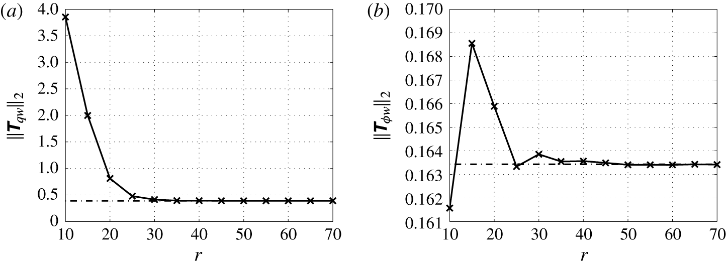
Performance of the ROM (
 $r=50$
). Magnitude frequency response from the state disturbance
 $w_{1}$
to the measured output
 $\unicode[STIX]{x1D708}_{1}$
(a) and from the control input
 $\unicode[STIX]{x1D719}_{1}$
to the controlled shear output
 $q_{1}$
(b) at the lower wall.
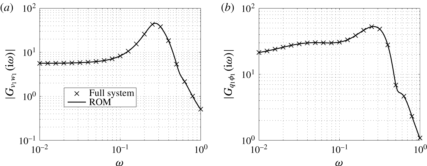
Contours of the closed-loop system norms
 $\Vert \unicode[STIX]{x1D64F}_{qw}\Vert _{2}$
(a),
 $\Vert \unicode[STIX]{x1D64F}_{\unicode[STIX]{x1D719}w}\Vert _{2}$
(b) and the relative energy norm
 $\Vert \unicode[STIX]{x1D64F}_{qw}\Vert _{2}^{2}/\Vert \unicode[STIX]{x1D642}_{qw}\Vert _{2}^{2}$
(c) with a
 $r=50$
reduced-order controller for different combinations of control parameter
 $l$
and estimation parameter
 $\unicode[STIX]{x1D6FE}$
(
 $\Vert \unicode[STIX]{x1D642}_{qw}\Vert _{2}=16.90$
). Controllers (I)
 $l=10$
,
 $\unicode[STIX]{x1D6FE}=1.5$
, (II)
 $l=20$
,
 $\unicode[STIX]{x1D6FE}=5$
and (III)
 $l=40$
,
 $\unicode[STIX]{x1D6FE}=15$
are considered for evaluating the closed-loop response of the system.

Figure 15 shows the contours of the
 ${\mathcal{H}}_{2}$
norms and the relative energy norm
 $\Vert \unicode[STIX]{x1D64F}_{qw}\Vert _{2}^{2}/\Vert \unicode[STIX]{x1D642}_{qw}\Vert _{2}^{2}$
for the order
 $r=50$
controller. It can be observed that an energy reduction between 90 %–99 % can easily be achieved by a proper choice of the design parameters. The performance for the case
 $l\rightarrow \infty ,\unicode[STIX]{x1D6FE}\rightarrow \infty$
converges to the uncontrolled case. The control penalty
 $l$
can be used to tune the feedback gain
 $\unicode[STIX]{x1D63E}_{K}$
in (3.9) and determines the trade-off between control effort and magnitude of the shear perturbation
 $\boldsymbol{q}$
. Lower values lead to an increased controller performance (low
 $\Vert \unicode[STIX]{x1D64F}_{qw}\Vert _{2}$
) at the cost of a higher control effort. It is found that choosing
 $l<10$
does lead to a significantly increase in performance. The parameter
 $\unicode[STIX]{x1D6FE}$
can be used to tune the estimator, that is the output injection gain
 $\unicode[STIX]{x1D63D}_{K}$
in (3.9). Low values for
 $\unicode[STIX]{x1D6FE}$
(high to noise ratio) lead to a higher magnitude of estimator feedback and an increased performance. However, choosing a lower value for
 $\unicode[STIX]{x1D6FE}$
leads to a reduced robustness. The role of
 $\unicode[STIX]{x1D6FE}$
is to account for uncertainties in the estimated output which also arise in the case of unmodelled dynamics and unmodelled disturbances. High estimator gain feedback can in this case result in larger overshoots which should be avoided since they can aggravate the initial stage to transition. From the contour of
 $\Vert \unicode[STIX]{x1D64F}_{qw}\Vert _{2}$
it can be observed that for a given control penalty
 $l$
, the estimation penalty
 $\unicode[STIX]{x1D6FE}$
, and thus the robustness, can be increased up to the curvature of the contour level without significant loss of performance. Thus choices for
 $l$
and
 $\unicode[STIX]{x1D6FE}$
on the curvature of a desired performance level can be considered as an optimal trade-off between robustness and the desired performance. In this study robustness is valued more than control effort in determining the trade-off. Three controllers will be investigated in the next sections for evaluating the performance in the frequency domain and through numerical simulation. The design parameters for the controllers are marked in figure 15. The first (I) is a high gain controller with
 $l=10$
,
 $\unicode[STIX]{x1D6FE}=1.5$
corresponding to approximately a 99.9 % energy reduction. The second (II) is an intermediate controller with
 $l=20$
,
 $\unicode[STIX]{x1D6FE}=5$
corresponding to a 99 % energy reduction and the third (III) is a lower gain controller with
 $l=40$
,
 $\unicode[STIX]{x1D6FE}=15$
corresponding to a 90 % energy reduction.
3.3 Closed-loop frequency response
In this section the three selected controllers are evaluated in the frequency domain. The magnitude frequency response from
 $w_{1}$
to the controlled output
 $q_{1}$
(2.7) is shown in figure 16. The magnitude of the closed-loop system
 $T_{q_{1}w_{1}}$
is compared with the magnitude of the open-loop system
 $G_{q_{1}w_{1}}$
. The frequency domain performance for the three controllers is in accordance with the results in figure 15. Controller (III) limits the control effort and takes higher levels of sensor inaccuracies into account. It is more conservative also with respect to higher frequencies. The three controllers significantly suppress the most amplified frequencies close to the design frequency
 $\unicode[STIX]{x1D714}=0.253$
as well as the off-design frequencies. The peak magnitude is equal to the
 ${\mathcal{H}}_{\infty }$
norm of
 $T_{q_{1}w_{1}}$
which is reduced between approximately 80 %–99 % for the three controllers.
The perturbation shear reduction along the complete walls, as well as spatial transients introduced by the control can be evaluated using the spatio-temporal frequency response. Figure 17 shows the magnitude for the shear along the lower wall for the open-loop system (a) and closed-loop (b) system with controller (II). Compared to the open-loop magnitude it can be observed that the controller significantly reduces the shear in the entire downstream region of the control actuators. The magnitude at the most dominant frequencies
 $0.1\leqslant \unicode[STIX]{x1D714}\leqslant 0.4$
is significantly suppressed and only small amplifications are present in the region of the control actuator.
Closed-loop frequency response from the inflow disturbance
 $w_{1}$
to the controlled output
 $q_{1}$
along the lower wall.
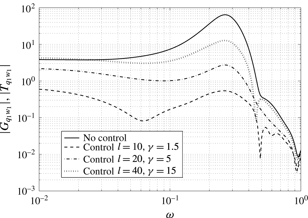
Open-loop (a) and closed-loop (b) magnitude frequency response from the inflow disturbance
 $w_{1}$
to the shear stress
 $\unicode[STIX]{x1D708}_{1}$
along the lower wall. The 10 contour levels lie within
 $|G_{\unicode[STIX]{x1D708}_{1}w_{1}}|,|T_{\unicode[STIX]{x1D708}_{1}w_{1}}|\in [6.9,~69.4]$
(
 $l=20$
,
 $\unicode[STIX]{x1D6FE}=5$
). The triangles indicate respectively the position of the measurement sensors (▿), the actuators (▵) and the controlled outputs (▹).
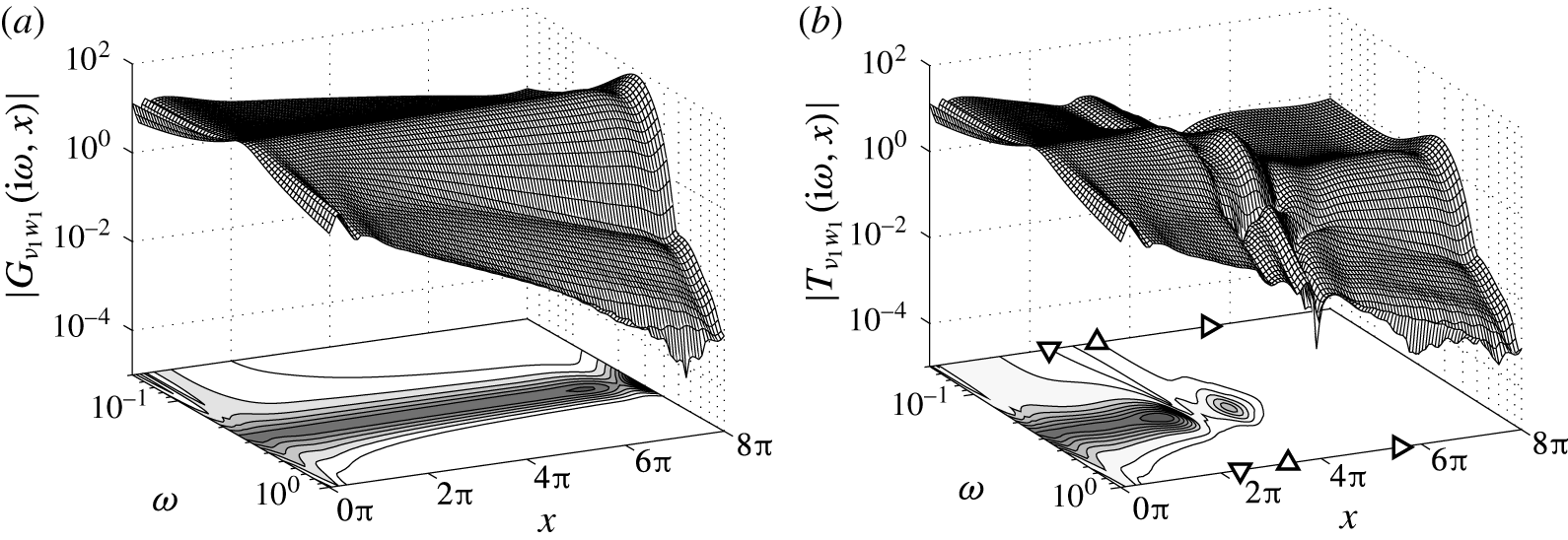
4 Closed-loop simulations
In this section the effectiveness of the proposed control design is evaluated using linear simulations of the closed-loop system. The three controllers characterised by (I)
 $l=10$
,
 $\unicode[STIX]{x1D6FE}=1.5$
, (II)
 $l=20$
,
 $\unicode[STIX]{x1D6FE}=5$
and (III)
 $l=40$
,
 $\unicode[STIX]{x1D6FE}=15$
are again considered, see also figure 15. The model defining a channel with a total length of
 $L_{sim}=16\unicode[STIX]{x03C0}$
, as discussed in § 2.5, is used for simulating the response. Disturbances are generated upstream of the control domain and propagate downstream. Three different disturbance cases are considered to demonstrate the robustness of the control design. In the first case (Case A, § 4.1), a single-frequency perturbation is considered which is generated using the disturbance model presented in § 2. This case can be seen as the design case, since the same disturbance model is used for both simulation and control design. In the second test case (case B, § 4.2) a multiple-frequency disturbance is considered in the form of a wave train consisting of a linear combination of Orr–Sommerfeld modes. This case is used to verify the spatio-temporal frequency domain results in the previous section and to test if the controller based on the single mode inflow disturbance model indeed allows for efficient estimation and control of perturbations in a wider frequency band. In the third test case (case C, § 4.3) the controller is evaluated for a stochastic excited body force located at the upper wall. Similar body forces have been used by Bagheri et al. (Reference Bagheri, Brandt and Henningson2009b
), Dadfar et al. (Reference Dadfar, Semeraro, Hanifi and Henningson2013) to evaluate controllers for transition delay. The case is used to study the effectiveness of the controller in a transient unmodelled environment. For simulating the response, the original unscaled system (2.24) is considered. For the design of the controller no a priori knowledge is assumed about the expected covariances
 $\unicode[STIX]{x1D70E}_{d}^{2}$
and
 $\unicode[STIX]{x1D70E}_{n}^{2}$
of respectively the state and measurement disturbances. Therefore, a scaling is introduced in terms of an expected relative magnitude of the sensor noise
 $\unicode[STIX]{x1D6FE}=\unicode[STIX]{x1D70E}_{n}/\unicode[STIX]{x1D70E}_{d}$
.
 $\unicode[STIX]{x1D6FE}$
plays a role for accounting measurement uncertainties in the control design and is not used for defining the measurement noise in the simulations. We also wish to investigate the robustness of the three controllers with respect to unmodelled measurement inaccuracies. Therefore each disturbance case is considered with both a low sensor noise
 $\unicode[STIX]{x1D70E}_{n}=0.01$
and a high sensor noise
 $\unicode[STIX]{x1D70E}_{n}=0.2$
. In total 18 different cases were simulated: three disturbance cases (A, B, C) with three controllers and two sensor noise intensities. The cases and the results are summarised in table 1 and are discussed in more detail in the next three sections.
The controlled shear output energy reduction and the control effort for three controllers. Three disturbance cases (A, B, C) are considered with both a low sensor noise (A1, B1, C1) and with a high sensor noise (A2, B2, C2). Each case is evaluated using three controllers (A1.I, A1.II, A1.III). Disturbance case A–C corresponds respectively to the single-frequency disturbance, multiple-frequency disturbance and stochastic in-domain forcing. (
 $\text{r.m.s.}~\unicode[STIX]{x1D753}=\sqrt{(1/T)\int _{0}^{T}|\unicode[STIX]{x1D753}|^{2}\,\text{d}t}$
).

Closed-loop performance for the single-frequency disturbance case. Controller (II) with low sensor noise is considered. (a) Shear measurements
 $\unicode[STIX]{x1D742}_{m}$
used for feedback. (b) Control input
 $\unicode[STIX]{x1D753}$
(amplitude of the blowing and suction). (c) Perturbation energy
 $E=\Vert \boldsymbol{u}\Vert _{L^{2}}^{2}$
. (d) Norm of the controlled perturbation shear output
 $\Vert \boldsymbol{q}\Vert _{2}$
.
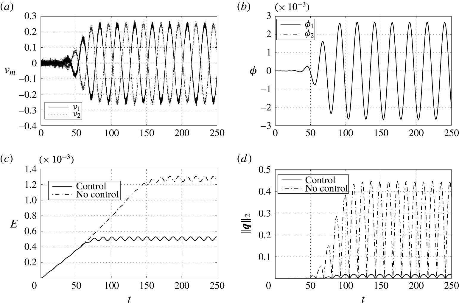
4.1 Case A: single-frequency disturbance
In the first case a single-frequency modal disturbance, of the form (2.9), is considered with
 $\unicode[STIX]{x1D714}=0.253$
which has the maximum growth rate for the investigated conditions. An animation of the controlled single-frequency disturbance is provided as supplementary movie 1, available at https://doi.org/10.1017/jfm.2017.355. This disturbance is generated at the inlet
 $x=-4\unicode[STIX]{x03C0}$
of the simulation domain using the disturbance model presented in § 2.2. The shape of the disturbance corresponds to the eigenfunction calculated from the Orr–Sommerfeld equation at
 $\unicode[STIX]{x1D714}=0.253$
(see figure 5). To mimic the transitional regime in the simulations the amplitude of the perturbation is set to
 $A_{0}=0.01$
. First the performance of controller (II) with
 $l=20$
,
 $\unicode[STIX]{x1D6FE}=5$
and a low sensor noise
 $\unicode[STIX]{x1D70E}_{n}=0.01$
is investigated. Figure 18 shows the temporal evolution of the shear measurements
 $\unicode[STIX]{x1D742}_{m}$
that are used for feedback, the control input
 $\unicode[STIX]{x1D753}$
(amplitude of the blowing and suction), the perturbation energy (
 $E=\Vert \boldsymbol{u}\Vert _{L^{2}}^{2}$
) and the norm of the controlled output
 $\Vert \boldsymbol{q}\Vert _{2}$
.
 $\boldsymbol{q}$
reflects the controller performance as it is used within the control objective that is minimised by the controller, see (2.29). As the perturbation convects downstream towards the control region, the amplitude of blowing and suction increases to cancel the perturbation. The effect of the noise on the shear measurements can be observed and the resulting control input confirms the filtering and feedback of these measurements. Both control actuators at the upper and lower wall act in phase which is to be expected due to the symmetry of the geometry and the control layout. A snapshot at
 $t=200$
of the flow perturbation field in the control domain
 $x\in [0,~8\unicode[STIX]{x03C0}]$
is shown in figure 19. The performance of the state estimation is best visualised without control applied. Figure 19(a) shows the estimated flow field without control, figure 19(b) shows the real flow field without control and figure 19(c) shows the real controlled flow. The estimated flow field is computed from the controller state
 $\boldsymbol{u}_{K}^{e}$
through
 $\boldsymbol{u}_{K}^{e}\mapsto \unicode[STIX]{x1D64E}_{r}^{-1}\boldsymbol{u}_{K}^{e}$
where
 $\unicode[STIX]{x1D64E}_{r}^{-1}$
are the first
 $r$
columns of the inverse of the similarity transformation as discussed in § 3.2. It can be seen that the flow perturbations are well reconstructed in the control region where the measurements are taken, actuation is applied and where the performance objective
 $\boldsymbol{q}$
is defined. As a result the controller is effective in cancelling the perturbations by minimising the effect of the perturbation on
 $\boldsymbol{q}$
. Only low-amplitude oscillations remain. The required amplitude of the blowing and suction is of the same order as the magnitude of the perturbation as can be seen in the snapshot for the wall-normal velocity component in figure 19(c).
To compare the performance of the three controllers, the spatial evolution of the perturbation is evaluated. We define the amplitude of the streamwise velocity perturbation as
 $$\begin{eqnarray}A(x)=\max _{t,y}\sqrt{|u|^{2}}.\end{eqnarray}$$
Figure 20 shows the amplitude for the three controllers with both low (
 $\unicode[STIX]{x1D70E}_{n}=0.01$
) and high (
 $\unicode[STIX]{x1D70E}_{n}=0.2$
) measurement noise. The amplitude reduction for the three controllers is in accordance with the frequency domain results in figure 16. The controllers are also robust to higher levels of sensor noise. Controller (III) takes higher sensor inaccuracies into account and the performance is preserved in the case of high sensor noise, see also table 1. Controllers (I) and (II) do not take such high measurement noise into account and the performance is less preserved. However, no severe deterioration can be observed. This can also be contributed to the simple structure of the perturbation.
Snapshot of the perturbation velocity within the control domain
 $x\in [0,~8\unicode[STIX]{x03C0}]$
at
 $t=200$
for the uncontrolled and controlled single frequency (
 $\unicode[STIX]{x1D714}=0.253$
) disturbance. Controller (II) with low sensor noise is considered. (a) Estimated velocity without control. (b) True velocity without control. (c) True velocity with control. The triangles indicate respectively the position of the measurement sensors (▿), the actuators (▵) and the controlled outputs (▹).
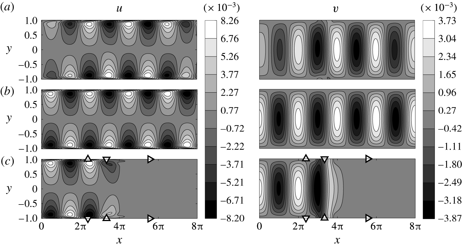
The maximum amplitude of the streamwise perturbation velocity (4.1) of the single-frequency disturbance for three controllers. (a) Feedback with low measurement noise
 $\unicode[STIX]{x1D70E}_{n}=0.01$
. (b) Feedback with high measurement noise
 $\unicode[STIX]{x1D70E}_{n}=0.2$
. The triangles indicate respectively the position of the measurement sensors (▿), the actuators (▵) and the controlled outputs (▹).

Spectrum of the multiple-frequency wavepacket for Case B.
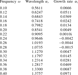
4.2 Case B: multiple-frequency disturbance
In the second test case a multiple-frequency disturbance is considered. An animation of the controlled multiple-frequency disturbance is provided as supplementary movie 2. The total disturbance consists of a linear combination of Orr–Sommerfeld modes. In total 16 modes in the frequency range
 $\unicode[STIX]{x1D714}\in [0.1,~0.4]$
are excited. Thus the disturbance is generated using 16 eigenfunctions whose shape corresponds to the eigenfunction calculated from the Orr–Sommerfeld equation at the selected frequencies. The temporal frequencies, the spatial wavelengths and spatial growth rates of these modes are listed in table 2. The spectrum includes 3 convectively unstable modes and 13 stable modes. Each mode is given the same amplitude
 $A_{0}=0.002$
such that the total disturbance is in the form of a wave train that is modulated as it propagates downstream. First the performance of controller (II) with a low sensor noise
 $\unicode[STIX]{x1D70E}_{n}=0.01$
is again investigated. The input–output signals and the closed-loop performance are shown in figure 21 and a snapshot at
 $t=200$
of the perturbation field in the control domain is shown in figure 22. The modulation of the perturbation can clearly be observed and the perturbation presents a richer structure as compared to the single-frequency case. With respect to the closed-loop performance the same observations can be made. The measurements are successfully filtered and the real flow is reconstructed well in the control domain as can be seen in figure 22. The controller is again able to cancel the perturbations and to suppress the perturbation wall shear stress. Although the unstable modes are dominant in the simulations, the (nearly) stable modes have not damped out and are still present as can be seen in figure 22. Nevertheless, the controller achieves nearly a full cancellation of the perturbations. This corroborates the findings of the input–output analysis presented in § 3.1 showing that the single mode disturbance model accurately captures the spatial wavelength and spatial growth of perturbations in a wider frequency band in the actuator/sensor region. As such the controller is able to effectively estimate and control a broader frequency spectrum of modes. To compare the performance of the three controllers, the spatial evolution of the perturbation is again evaluated. Since the amplitude of the perturbation also varies in time a measure for the time-averaged amplitude is defined
 $$\begin{eqnarray}\bar{A}(x)=\max _{y}\sqrt{\frac{1}{T}\int _{0}^{T}|u|^{2}\,\text{d}t},\end{eqnarray}$$
which is the wall-normal maximum amplitude of the root mean square (r.m.s.) streamwise velocity perturbation (Andersson, Berggren & Henningson Reference Andersson, Berggren and Henningson1999). Figure 23 shows the time-averaged amplitude for the three controllers with both low and high measurements noise. It can be observed that the amplitude reduction in case of high measurement noise for controller (I) is reduced more significantly. This is to be expected since the controller does not take high measurement inaccuracies into account. However, it still achieves a robust performance. Actually controller (I) and (II) have a comparable performance, see also table 1. This indicates that there is no large sensitivity in the choice of design parameters in case of high sensor noise. Again, the performance of controller (III) is preserved and is in accordance with its design.
Closed-loop performance for the multiple-frequency disturbance case. Controller (II) with low sensor noise is considered. (a) Shear measurements
 $\unicode[STIX]{x1D742}_{m}$
used for feedback. (b) Control input
 $\unicode[STIX]{x1D753}$
. (c) Perturbation energy
 $E=\Vert \boldsymbol{u}\Vert _{L^{2}}^{2}$
. (d) Norm of the controlled perturbation shear output
 $\Vert \boldsymbol{q}\Vert _{2}$
.

Snapshot of the perturbation velocity within the control domain
 $x\in [0,~8\unicode[STIX]{x03C0}]$
at
 $t=200$
for the uncontrolled and controlled multiple-frequency disturbance. Controller (II) with low sensor noise is considered. (a) Estimated velocity without control. (b) True velocity without control. (c) True velocity with control. The triangles indicate respectively the position of the measurement sensors (▿), the actuators (▵) and the controlled outputs (▹).

The wall-normal maximum amplitude of the root mean square streamwise perturbation velocity (4.2) of the multiple-frequency disturbance for three controllers. (a) Feedback with low measurement noise
 $\unicode[STIX]{x1D70E}_{n}=0.01$
. (b) Feedback with high measurement noise
 $\unicode[STIX]{x1D70E}_{n}=0.2$
. The triangles indicate respectively the position of the measurement sensors (▿), the actuators (▵) and the controlled outputs (▹).
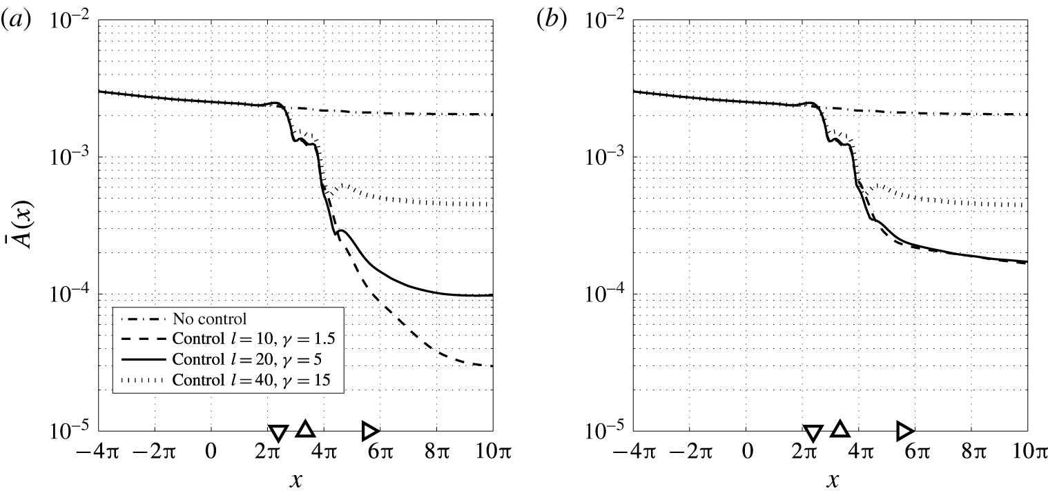
Contours of the spatial distribution
 $\boldsymbol{F}=[F_{x},~F_{y}]^{\text{T}}$
of the in-domain disturbance used for case C.
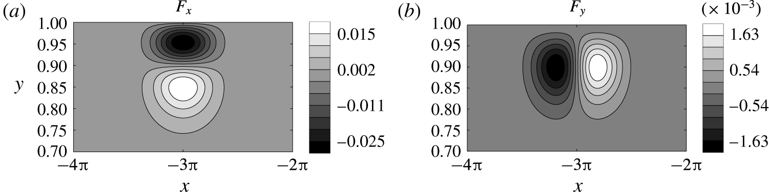
4.3 Case C: stochastic in-domain forcing
In the third most challenging test case a stochastic in-domain forcing is considered which is generated at the upper wall near the inflow. An animation of the controlled stochastic in-domain forcing is provided as supplementary movie 3. In this case the momentum equation is forced with
 $$\begin{eqnarray}\boldsymbol{f}(x,y,t)=\boldsymbol{F}(x,y)w(t),\end{eqnarray}$$
where
 $w(t)$
is zero mean white noise with a normal distribution at unit intensity. The spatial distribution of the ‘vibrating ribbon’ at the upper wall
 $(y=1)$
corresponds to that of Bertolotti, Herbert & Spalart (Reference Bertolotti, Herbert and Spalart1992) and has the form
 $F_{x}=\unicode[STIX]{x2202}\unicode[STIX]{x1D713}/\unicode[STIX]{x2202}y$
,
 $F_{y}=-\unicode[STIX]{x2202}\unicode[STIX]{x1D713}/\unicode[STIX]{x2202}x$
with
 $$\begin{eqnarray}\unicode[STIX]{x1D713}(x,y)=\unicode[STIX]{x1D716}\exp \left(-\frac{(x-x_{r})^{2}}{\unicode[STIX]{x1D70E}_{x}^{2}}-\frac{(y-1)^{2}}{\unicode[STIX]{x1D70E}_{y}^{2}}\right)(y-1)^{2}\cos ((x-x_{r})),\end{eqnarray}$$
where
 $\unicode[STIX]{x1D716}=0.5$
is the amplitude of the force,
 $\unicode[STIX]{x1D70E}_{x}=1$
,
 $\unicode[STIX]{x1D70E}_{y}=0.1$
the spatial lengths,
 $x_{r}=-3\unicode[STIX]{x03C0}$
the
 $x$
-position of the ribbon. The spatial distribution of this force is shown in figure 24. The body force (
 $F_{x},F_{y}$
) is both divergence free and satisfies the no-slip boundary conditions. First the performance of controller (II) with a low sensor noise is investigated. The input–output signals and the closed-loop performance are shown in figure 25 and a snapshot at
 $t=350$
of the perturbation field in the control domain is shown in figure 26. In addition, to better visualise the evolution of the perturbation and the controller performance, the temporal evolution for the shear stress along the lower wall for the uncontrolled case and the controlled case is shown in figure 27.
Closed-loop performance for the stochastic disturbance case. Controller (II) with low sensor noise is considered. (a) Shear measurements
 $\unicode[STIX]{x1D742}_{m}$
used for feedback. (b) Control input
 $\unicode[STIX]{x1D753}$
. (c) Perturbation energy
 $E=\Vert \boldsymbol{u}\Vert _{L^{2}}^{2}$
. (d) Norm of the controlled perturbation shear output
 $\Vert \boldsymbol{q}\Vert _{2}$
.
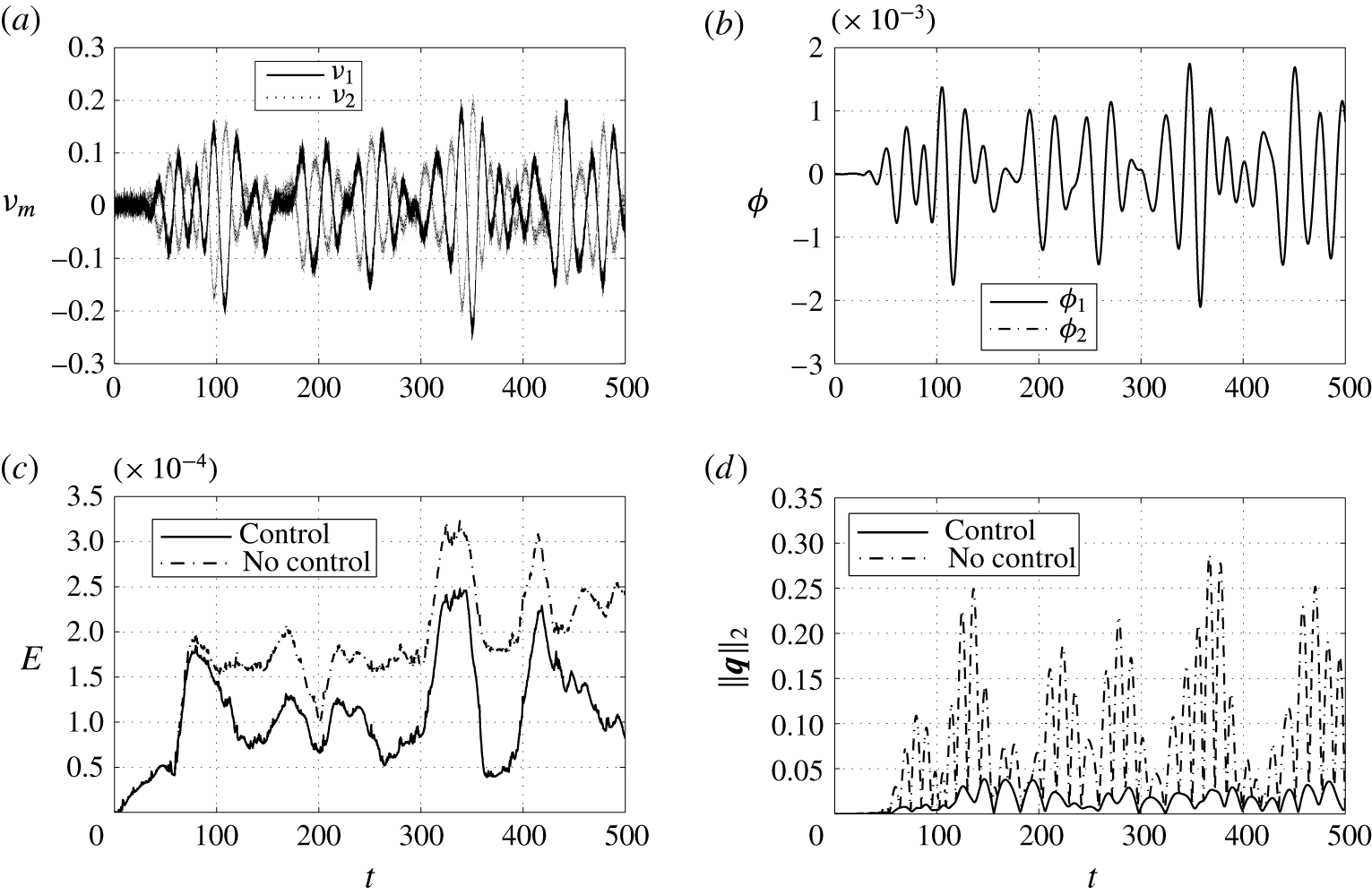
Snapshot of the perturbation velocity within the control domain
 $x\in [0,~8\unicode[STIX]{x03C0}]$
at
 $t=350$
for the uncontrolled and controlled stochastic disturbance. Controller (II) with low sensor noise is considered. (a) Estimated velocity without control. (b) True velocity without control. (c) True velocity with control. The triangles indicate respectively the position of the measurement sensors (▿), the actuators (▵) and the controlled outputs (▹).

Temporal evolution of the wall shear stress
 $\unicode[STIX]{x2202}u/\unicode[STIX]{x2202}y$
along the bottom wall of the channel for the stochastic forced disturbance. The triangles indicate respectively the position of the measurement sensors (▿), the actuators (▵) and the controlled outputs (▹).

The wall-normal maximum amplitude of the r.m.s. streamwise perturbation velocity (4.2) of the stochastic forced disturbance for three controllers. (a) Feedback with low measurement noise
 $\unicode[STIX]{x1D70E}_{n}=0.01$
. (b) Feedback with high measurement noise
 $\unicode[STIX]{x1D70E}_{n}=0.2$
. The triangles indicate respectively the position of the measurement sensors (▿), the actuators (▵) and the controlled outputs (▹).
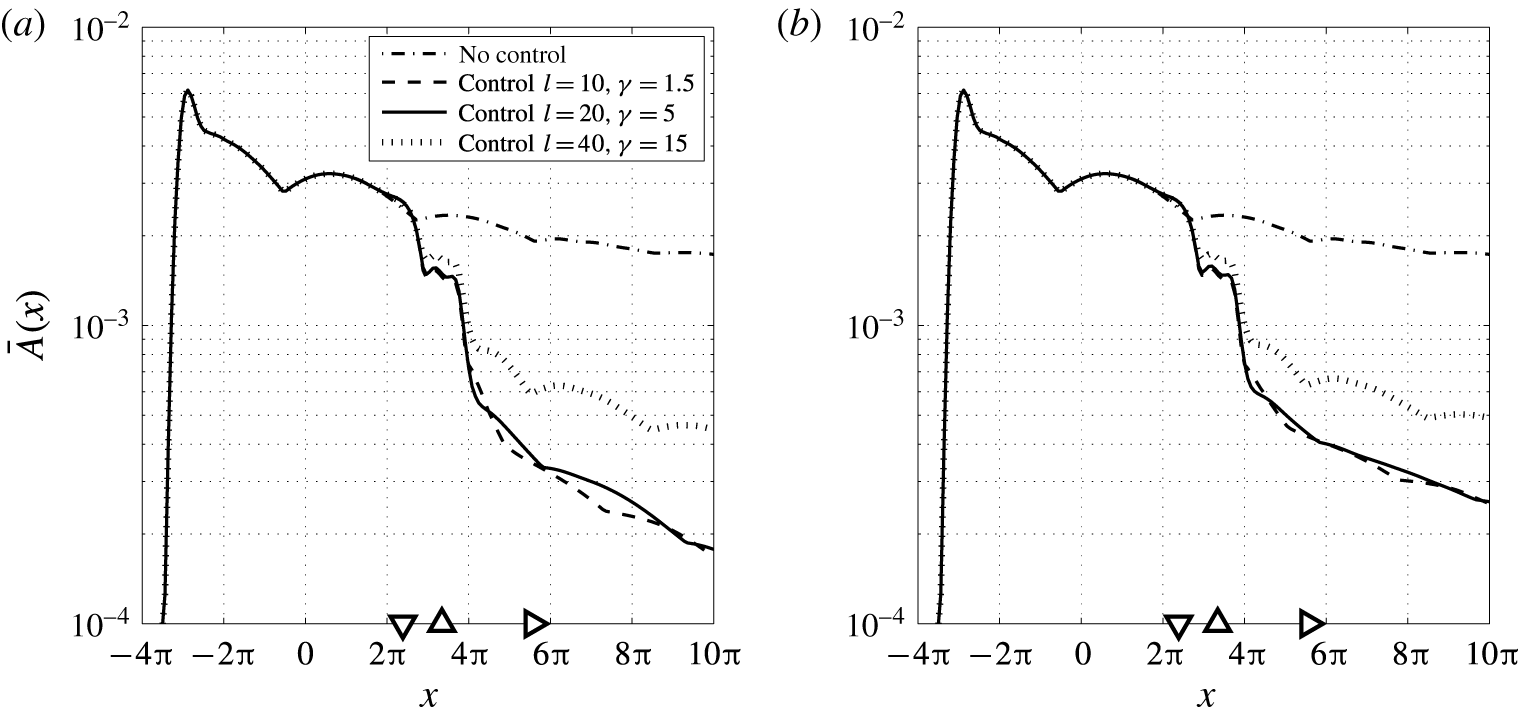
The stochastic disturbance excites a spectrum of frequencies which results in large initial transients after which the disturbance develops in the form of wavepackets as can be seen in the energy plot in figure 25. The transients can also observed in the temporal evolution of the wall shear stress in figure 27 and are also present in the control region. It can be observed that the controller is still able to properly estimate the flow field and is effective in both minimising the wall shear stress and reducing the perturbation energy in the domain. Although a complete cancellation of the disturbance is not possible, the controller manages to achieve a reduction of 97 % in the controlled shear output power, see also table 1. Note that the disturbance is completely independent of the disturbance model used to design the controller. It is defined in-domain and creates initially asymmetric developing perturbations while the complete input–output layout is symmetric. Furthermore the transients are not accounted for in the control design and the perturbations are not fully developed in the control domain. Nevertheless, the controller achieves a high level of robustness to unmodelled disturbances; no overshoots can be observed in the perturbation energy and the controlled output, and the controller does not aggravate the flow. This can be contributed to the fact that the controller is able to estimate and stabilise the underlying modes that are present in the disturbance as can be seen from figure 26.
Figure 28 shows the time-averaged amplitude for the three controllers with both low and high measurements noise. It can be observed that controllers (I) and (II) have comparable performance, also for the low sensor noise case. This can be contributed to the fact that uncertainties in output measurements also arise due to the unmodelled disturbances. This indicates that there is also no large sensitivity in the choice of design parameters in case of unmodelled disturbances.
5 Conclusion
The paper presents a new framework to design and synthesise
 ${\mathcal{H}}_{2}$
optimal controllers for control of linear instabilities in 2-D laminar wall-bounded shear flows. The 2-D non-periodic channel flow is considered as a case study. The flow modelling accounts both for localised actuation/sensing and the dominant perturbation dynamics in physical space. A new inflow disturbance model is presented for external sources of excitation. This model allows for an efficient estimation of the flow perturbations in the localised control domain using wall shear sensors. The perturbation modes that contribute to transition can be selected and are included in the control design. In this way the most dominant modes of the flow can be precisely targeted by the controller. A reduced-order model (
 $r=50$
) that captures the input–output behaviour is derived directly from the linearised Navier–Stokes equations using exact balanced truncation. No numerical simulations are required to synthesise the controller. The reduced-order model is used to design an
 ${\mathcal{H}}_{2}$
optimal controller to minimise the wall shear stress created by the perturbations. It is shown that there is no loss in performance due to the truncated dynamics and the reduced-order controller maintains the closed-loop performance as compared to the full-order controller. The controller is evaluated with linear simulations of the closed-loop system. Three different disturbance cases are considered to evaluate the effectiveness and robustness of the proposed control design. It is shown that the controller is able to cancel the perturbations and is robust to both unmodelled disturbances and sensor inaccuracies.
The modelling presented in this paper provides an efficient means to design and synthesise controllers directly from the governing equations. This can be contributed to the fact that the aim is to capture the input–output behaviour for localised sensors and actuators, and the dominant perturbation dynamics within this localised region. It is shown that with the new inflow disturbance model only minor spatial transients are involved for the perturbation modes to develop in the domain. This allows an arbitrary placement of the computational inflow boundary as it does not affect the spatial length scales of the perturbations in the control region. Small computational domains can thus be used to create the control models. Furthermore, to achieve effective control it is not required to fully resolve the flow at all length scales in the initial model. Only the dominant modes that contribute to transition and are included in the control design should be accurately resolved. These features can make the extension to three dimensions computationally feasible. Transition in 3-D flows is also governed by algebraic growth of non-modal perturbations, which bypasses the classical transition scenario considered in this study. To effectively apply this method to 3-D flows requires the inclusion of multiple perturbation modes at different wavenumbers in the disturbance model or the use of optimal inflow perturbations, e.g. of the form presented in Andersson et al. (Reference Andersson, Berggren and Henningson1999). In this paper multivariate splines are used in the underlying numerical method which are effective in creating control models. Multivariate splines are defined on triangulations allowing to approximate any domain and to use local refinements in regions of interest. Secondly, they are general in terms of smoothness and degree allowing for a higher resolving power. It is also worth noting that the framework is generalised, independently of the spatial discretisation method used in this study.
Significant work remains to be done to apply this method in real life applications. We are currently extending this method for control of Tollmien–Schlichting waves in spatially developing boundary layer flows and are working towards experimental validation of this method in the wind tunnel. Future work will focus on the application for efficient modelling and control of 3-D disturbances. This paper focussed on optimal control and no other model uncertainties, such as input/actuator uncertainties and uncertainties in the Reynolds number were addressed. Recently in Fabbiane et al. (Reference Fabbiane, Simon, Fischer, Grundmann, Bagheri and Henningson2015) it is shown through experiments that deviations from the design conditions can destabilise optimal controllers. Future work will also focus on addressing model uncertainties by integrating this method in a
 ${\mathcal{H}}_{\infty }$
robust control framework.
Acknowledgements
This work is partially supported by NSF awards ECCS-1408442 and CMMI-1363386.
Supplementary movies
Supplementary movies are available at https://doi.org/10.1017/jfm.2017.355.
Appendix A. Multivariate spline state-space representation of the flow
In this section the finite-dimensional state-space system for the flow control problem is derived. This method uses multivariate splines defined on triangulation’s (Farin Reference Farin1986; de Boor Reference de Boor and Farin1987; Lai & Schumaker Reference Lai and Schumaker2007) to find matrix representations of all operators in (2.23) and applies to general geometries and general control configurations. This method is an extension of the model reduction scheme for parabolic PDEs presented by Tol et al. (Reference Tol, de Visser and Kotsonis2016) to fluid flows. In Awanou & Lai (Reference Awanou and Lai2004) a numerical scheme is presented for approximating steady Navier–Stokes equations in velocity pressure formulation using multivariate splines. This numerical scheme is combined with the framework from Tol et al. (Reference Tol, de Visser and Kotsonis2016) to derive state descriptions for the linearised Navier–Stokes equations and is presented § A.1. The state-space system for the case of the non-periodic channel flow was validated in § 3 by comparing the spatial stability with the predictions from LST. For completeness and to mathematically verify the numerical method, the state-space system for the case of the periodic channel flow is validated using the temporal stability theory in § A.2.
A.1 Numerical method
In this appendix the state equations are considered which are given by the forced LNSE
 $$\begin{eqnarray}\displaystyle & \displaystyle \frac{\unicode[STIX]{x2202}\boldsymbol{u}}{\unicode[STIX]{x2202}t}+(\boldsymbol{U}\boldsymbol{\cdot }\unicode[STIX]{x1D735})\boldsymbol{u}+(\boldsymbol{u}\boldsymbol{\cdot }\unicode[STIX]{x1D735})\boldsymbol{U}-\frac{1}{Re}\unicode[STIX]{x0394}\boldsymbol{u}+\unicode[STIX]{x1D735}p=\boldsymbol{f}\quad \text{in}~\unicode[STIX]{x1D6FA}, & \displaystyle\end{eqnarray}$$
 $$\begin{eqnarray}\displaystyle & \unicode[STIX]{x1D735}\boldsymbol{\cdot }\boldsymbol{u}=0\quad \text{in}~\unicode[STIX]{x1D6FA}, & \displaystyle\end{eqnarray}$$
 $$\begin{eqnarray}\displaystyle & \boldsymbol{u}=\boldsymbol{u}_{b}\quad \text{on}~\unicode[STIX]{x1D6E4}_{D}, & \displaystyle\end{eqnarray}$$
 $$\begin{eqnarray}\displaystyle & \displaystyle -p\boldsymbol{n}+\frac{1}{Re}(\boldsymbol{n}\boldsymbol{\cdot }\unicode[STIX]{x1D735})\boldsymbol{u}=0\quad \text{on}~\unicode[STIX]{x1D6E4}_{out}. & \displaystyle\end{eqnarray}$$
 $L^{2}(\unicode[STIX]{x1D6FA})$
be the space of square integrable functions over
 $\unicode[STIX]{x1D6FA}$
. We define the following Sobolev spaces
 $$\begin{eqnarray}\displaystyle \left.\begin{array}{@{}c@{}}\displaystyle H^{1}(\unicode[STIX]{x1D6FA})=\left\{u\in L^{2}(\unicode[STIX]{x1D6FA}),\frac{\unicode[STIX]{x2202}u}{\unicode[STIX]{x2202}x_{i}}\in L^{2}(\unicode[STIX]{x1D6FA})~\text{for}~i=1,\ldots ,n\right\},\\ H_{0}^{1}(\unicode[STIX]{x1D6FA})=\{u\in H^{1}(\unicode[STIX]{x1D6FA}),~u|_{\unicode[STIX]{x1D6E4}_{D}}=0\}.\end{array}\right\} & & \displaystyle\end{eqnarray}$$
 $H^{1}(\unicode[STIX]{x1D6FA})$
consists of square integrable functions whose first-order derivative exists in the weak sense and
 $H_{0}^{1}(\unicode[STIX]{x1D6FA})$
is the subspace in which the functions vanish on the Dirichlet portion of the boundary
 $\unicode[STIX]{x1D6E4}_{D}$
. For vector valued functions the notation
 $\boldsymbol{H}^{1}(\unicode[STIX]{x1D6FA})=H^{1}(\unicode[STIX]{x1D6FA})^{n}$
is used. We define the bilinear form
 $$\begin{eqnarray}a(\boldsymbol{v},\boldsymbol{u})=\frac{1}{Re}\int _{\unicode[STIX]{x1D6FA}}\unicode[STIX]{x1D735}\boldsymbol{v}\boldsymbol{ : }\unicode[STIX]{x1D735}\boldsymbol{u}\,\text{d}\unicode[STIX]{x1D6FA}=:\frac{1}{Re}\int _{\unicode[STIX]{x1D6FA}}\mathop{\sum }_{i=1}^{n}\mathop{\sum }_{j=1}^{n}\frac{\unicode[STIX]{x2202}u_{i}}{\unicode[STIX]{x2202}x_{j}}\frac{\unicode[STIX]{x2202}v_{i}}{\unicode[STIX]{x2202}x_{j}}\,\text{d}\unicode[STIX]{x1D6FA}\quad \forall ~\boldsymbol{v},\boldsymbol{u}\in \boldsymbol{H}^{1}(\unicode[STIX]{x1D6FA})\end{eqnarray}$$
and the trilinear form
 $$\begin{eqnarray}b(\boldsymbol{v},\boldsymbol{u},\boldsymbol{w})=\int _{\unicode[STIX]{x1D6FA}}\boldsymbol{v}\boldsymbol{\cdot }(\boldsymbol{u}\boldsymbol{\cdot }\unicode[STIX]{x1D735})\boldsymbol{w}\,\text{d}\unicode[STIX]{x1D6FA}=\int _{\unicode[STIX]{x1D6FA}}\mathop{\sum }_{i=1}^{n}\mathop{\sum }_{j=1}^{n}v_{i}u_{j}\frac{\unicode[STIX]{x2202}w_{i}}{\unicode[STIX]{x2202}x_{j}}\,\text{d}\unicode[STIX]{x1D6FA}\quad \forall ~\boldsymbol{v},\boldsymbol{u},\boldsymbol{w}\in \boldsymbol{H}^{1}(\unicode[STIX]{x1D6FA}).\end{eqnarray}$$
Also the inner product for functions belonging to
 $\boldsymbol{L}^{2}(\unicode[STIX]{x1D6FA})$
is given by
 $$\begin{eqnarray}(\boldsymbol{v},\boldsymbol{u})=\int _{\unicode[STIX]{x1D6FA}}\boldsymbol{v}\boldsymbol{\cdot }\boldsymbol{u}\,\text{d}\unicode[STIX]{x1D6FA}.\end{eqnarray}$$
Equation (2.1) has no dynamic equation for the pressure that can be utilised for control. Therefore the pressure is eliminated from the equations by using a space of velocity fields which are exactly divergence free. Let
 $$\begin{eqnarray}\displaystyle \left.\begin{array}{@{}c@{}}\boldsymbol{V}_{0}=\{\boldsymbol{v}\in \boldsymbol{H}_{0}^{1}(\unicode[STIX]{x1D6FA}),\unicode[STIX]{x1D735}\boldsymbol{\cdot }\boldsymbol{v}=0\},\\ \boldsymbol{V}_{g}=\{\boldsymbol{u}\in \boldsymbol{H}^{1}(\unicode[STIX]{x1D6FA}),\boldsymbol{u}|_{\unicode[STIX]{x1D6E4}_{D}}=\boldsymbol{u}_{b},\unicode[STIX]{x1D735}\boldsymbol{\cdot }\boldsymbol{u}=0\}.\end{array}\right\} & & \displaystyle\end{eqnarray}$$
The weak form of (A 1) can be obtained by taking the inner product of the first equation (A 1a
) with
 $\boldsymbol{v}\in \boldsymbol{V}_{0}$
 $$\begin{eqnarray}\int _{\unicode[STIX]{x1D6FA}}\left\{\boldsymbol{v}\boldsymbol{\cdot }\frac{\unicode[STIX]{x2202}\boldsymbol{u}}{\unicode[STIX]{x2202}t}-\frac{1}{Re}\boldsymbol{v}\boldsymbol{\cdot }\unicode[STIX]{x0394}\boldsymbol{u}+\boldsymbol{v}\boldsymbol{\cdot }(\boldsymbol{U}\boldsymbol{\cdot }\unicode[STIX]{x1D735})\boldsymbol{u}+\boldsymbol{v}\boldsymbol{\cdot }(\boldsymbol{u}\boldsymbol{\cdot }\unicode[STIX]{x1D735})\boldsymbol{U}+\boldsymbol{v}\boldsymbol{\cdot }\unicode[STIX]{x1D735}p\right\}\text{d}\unicode[STIX]{x1D6FA}=\int _{\unicode[STIX]{x1D6FA}}\boldsymbol{v}\boldsymbol{\cdot }\boldsymbol{f}\,\text{d}\unicode[STIX]{x1D6FA}.\end{eqnarray}$$
Applying integration by parts and the divergence theorem to the diffusion term and the pressure gradient term gives
 $$\begin{eqnarray}\displaystyle & & \displaystyle \int _{\unicode[STIX]{x1D6FA}}\left\{\boldsymbol{v}\boldsymbol{\cdot }\frac{\unicode[STIX]{x2202}\boldsymbol{u}}{\unicode[STIX]{x2202}t}+\frac{1}{Re}\unicode[STIX]{x1D735}\boldsymbol{v}\boldsymbol{ : }\unicode[STIX]{x1D735}\boldsymbol{u}+\boldsymbol{v}\boldsymbol{\cdot }(\boldsymbol{U}\boldsymbol{\cdot }\unicode[STIX]{x1D735})\boldsymbol{u}+\boldsymbol{v}\boldsymbol{\cdot }(\boldsymbol{u}\boldsymbol{\cdot }\unicode[STIX]{x1D735})\boldsymbol{U}-p(\unicode[STIX]{x1D735}\boldsymbol{\cdot }\boldsymbol{v})\right\}\text{d}\unicode[STIX]{x1D6FA}\nonumber\\ \displaystyle & & \displaystyle \qquad -\,\int _{\unicode[STIX]{x1D6E4}_{D}}\boldsymbol{v}\boldsymbol{\cdot }\left(-p\boldsymbol{n}+\frac{1}{Re}(\boldsymbol{n}\boldsymbol{\cdot }\unicode[STIX]{x1D735})\boldsymbol{u}\right)\,\text{d}\unicode[STIX]{x1D6E4}-\int _{\unicode[STIX]{x1D6E4}_{out}}\boldsymbol{v}\boldsymbol{\cdot }\left(-p\boldsymbol{n}+\frac{1}{Re}(\boldsymbol{n}\boldsymbol{\cdot }\unicode[STIX]{x1D735})\boldsymbol{u}\right)\text{d}\unicode[STIX]{x1D6E4}\nonumber\\ \displaystyle & & \displaystyle \quad =\int _{\unicode[STIX]{x1D6FA}}\boldsymbol{v}\boldsymbol{\cdot }\boldsymbol{f}\,\text{d}\unicode[STIX]{x1D6FA}.\end{eqnarray}$$
The Neumann outflow boundary condition (A 1d
) occurs in (A 8) as a boundary integral term and can therefore naturally be imposed by setting it to zero. Furthermore,
 $\unicode[STIX]{x1D735}\boldsymbol{\cdot }\boldsymbol{v}=0$
and
 $\boldsymbol{v}|_{\unicode[STIX]{x1D6E4}_{D}}=0$
for all
 $\boldsymbol{v}\in \boldsymbol{V}_{0}$
. The variational formulation of the problem (A 1) can thus be stated as: find
 $\boldsymbol{u}\in L^{2}(0,T;\boldsymbol{V}_{g})$
such that
 $$\begin{eqnarray}\displaystyle \left(\boldsymbol{v},\frac{\unicode[STIX]{x2202}\boldsymbol{u}}{\unicode[STIX]{x2202}t}\right)+a(\boldsymbol{v},\boldsymbol{u})+b(\boldsymbol{v},\boldsymbol{U},\boldsymbol{u})+b(\boldsymbol{v},\boldsymbol{u},\boldsymbol{U})=(\boldsymbol{v},\boldsymbol{f})\quad \forall ~\boldsymbol{v}\in \boldsymbol{V}_{0}. & & \displaystyle\end{eqnarray}$$
The multivariate spline space is used as approximating space for the velocity. Let
 ${\mathcal{T}}$
be the triangulation (triangular mesh) of the domain
 $\unicode[STIX]{x1D6FA}$
. The spline space is the space of all smooth piecewise polynomial functions of arbitrary degree
 $d$
and arbitrary smoothness
 $r$
over
 ${\mathcal{T}}$
with
 $0\leqslant r<d$
 $$\begin{eqnarray}S_{d}^{r}({\mathcal{T}}):=s\in C^{r}(\unicode[STIX]{x1D6FA}),s|_{t}\in {\mathcal{P}}_{d},\quad \forall t\in {\mathcal{T}}.\end{eqnarray}$$
With
 ${\mathcal{P}}_{d}$
the space of all polynomials of total degree
 $d$
and
 $t$
denotes a triangle. To approximate the velocity vector
 $\boldsymbol{u}=(u,v)$
we use
 $\boldsymbol{s}_{\boldsymbol{u}}=(s_{1},s_{2})\in \boldsymbol{S}_{g}$
with
 $\boldsymbol{S}_{g}=S_{d}^{r}({\mathcal{T}})^{2}\cap \boldsymbol{V}_{g}$
. The spline approximation of (A 9) is to seek
 $\boldsymbol{s}_{\boldsymbol{u}}(\cdot ,t)\in \boldsymbol{S}_{g}\subset \boldsymbol{V}_{g}$
such that
 $$\begin{eqnarray}\displaystyle \left(\boldsymbol{s}_{v},\frac{\unicode[STIX]{x2202}\boldsymbol{s}_{\boldsymbol{u}}}{\unicode[STIX]{x2202}t}\right)+a(\boldsymbol{s}_{v},\boldsymbol{s}_{\boldsymbol{u}})+b(\boldsymbol{s}_{v},\boldsymbol{U},\boldsymbol{s}_{\boldsymbol{u}})+b(\boldsymbol{s}_{v},\boldsymbol{s}_{\boldsymbol{u}},\boldsymbol{U})=(\boldsymbol{s}_{v},\boldsymbol{f})\quad \forall ~\boldsymbol{s}_{v}\in \boldsymbol{S}_{0}. & & \displaystyle\end{eqnarray}$$
After constructing a basis for
 $\boldsymbol{S}_{0}$
and
 $\boldsymbol{S}_{g}$
, equation (A 11) is equivalent to a system of ordinary differential equations. However, the implementation of such divergence free spline elements of arbitrary degree and smoothness is very complicated. Awanou & Lai (Reference Awanou and Lai2004) streamlined this process by skipping the construction of smooth divergence free finite elements. Instead, they used discontinuous piecewise polynomial functions over a triangulation and treated desired smoothness properties together with the boundary conditions and the incompressibility condition as side constraints. This approach is also applied here to the time dependent problem (A 11). The multivariate spline function is represented using the B-form of splines (Farin Reference Farin1986; de Boor Reference de Boor and Farin1987). We use the vector formulation from de Visser, Chu & Mulder (Reference de Visser, Chu and Mulder2009)
 $$\begin{eqnarray}s_{i}(\boldsymbol{x},t)=\unicode[STIX]{x1D63D}^{d}(\boldsymbol{x})\boldsymbol{c}_{i}(t),\end{eqnarray}$$
with
 $\unicode[STIX]{x1D63D}^{d}(\boldsymbol{x})\in \mathbb{R}^{1\times \cdot n_{e}\hat{d}}$
the global vector of B-form basis polynomials,
 $n_{e}$
the number of elements in
 ${\mathcal{T}}$
and
 $\hat{d}=\binom{n}{n+d}$
the number of basis polynomials per element. The spline function is identified by its B-coefficient vector
 $\boldsymbol{c}_{i}(t)\in \mathbb{R}^{n_{e}\hat{d}\times 1}$
which are used as the time-varying expansion coefficients. Since
 $s$
has a certain smoothness, the smoothness conditions can be expressed by a linear system (Awanou et al.
Reference Awanou, Lai, Wenston, Chen and Lai2005) and (Lai & Schumaker Reference Lai and Schumaker2007, pp. 133–135). That is
 $s\in C^{r}$
if and only if
 $$\begin{eqnarray}\unicode[STIX]{x1D643}\boldsymbol{c}_{i}=\mathbf{0}.\end{eqnarray}$$
Constructing
 $\unicode[STIX]{x1D643}$
is not trivial and we refer to de Visser et al. (Reference de Visser, Chu and Mulder2009) for a general formulation of the continuity conditions and the procedure to derive them. The Dirichlet boundary condition (A 1c
) provides additional constraints on the B-coefficient vector. For control application the boundary condition is of the form
 $\boldsymbol{u}|_{\unicode[STIX]{x1D6E4}_{D}}=\boldsymbol{u}_{b}(\boldsymbol{x},t)=[g_{1}(\boldsymbol{x}),g_{2}(\boldsymbol{x})]^{\text{T}}\unicode[STIX]{x1D719}_{\unicode[STIX]{x1D6E4}}(t)$
with
 $g_{i}(\boldsymbol{x})$
the spatial distribution function for the
 $i$
th velocity component and
 $\unicode[STIX]{x1D719}_{\unicode[STIX]{x1D6E4}}(t)$
the temporal boundary control input. The discrete constraints for this condition can also be given by a linear system (Awanou & Lai Reference Awanou and Lai2004; Tol et al.
Reference Tol, de Visser and Kotsonis2016)
 $$\begin{eqnarray}\unicode[STIX]{x1D64D}\boldsymbol{c}_{i}=\boldsymbol{G}_{i}\unicode[STIX]{x1D719}_{\unicode[STIX]{x1D6E4}}.\end{eqnarray}$$
Where
 $\boldsymbol{G}_{i}$
is a vector of B-coefficients that interpolates
 $g_{i}(\boldsymbol{x})$
at the boundary
 $\unicode[STIX]{x1D6E4}_{D}$
. The function
 $s\in C^{r}(\unicode[STIX]{x1D6FA})$
is guaranteed to be
 $r$
times continuously differentiable on the domain
 $\unicode[STIX]{x1D6FA}$
. To approximate the variational formulation only first-order derivatives are required. There exist matrices
 $\unicode[STIX]{x1D63F}_{i}$
(Awanou & Lai Reference Awanou and Lai2004; de Visser, Chu & Mulder Reference de Visser, Chu and Mulder2011) which map the B-coefficient vector of any spline function
 $s\in S_{d}^{r}({\mathcal{T}})$
to the B-coefficient vector of
 $(\unicode[STIX]{x2202}/\unicode[STIX]{x2202}x_{i})s$
, that is
 $$\begin{eqnarray}\frac{\unicode[STIX]{x2202}}{\unicode[STIX]{x2202}x_{i}}[\unicode[STIX]{x1D63D}^{d}(\boldsymbol{x})\boldsymbol{c}]=\unicode[STIX]{x1D63D}^{d-1}(\boldsymbol{x})\unicode[STIX]{x1D63F}_{i}\boldsymbol{c}.\end{eqnarray}$$
The spline approximation
 $\boldsymbol{s}_{\boldsymbol{u}}=(s_{1},s_{2})$
is identified with B-coefficients
 $\boldsymbol{c}=(\boldsymbol{c}_{1},\boldsymbol{c}_{2})$
. Hence the discrete equivalent of
 $\unicode[STIX]{x1D735}\boldsymbol{\cdot }\boldsymbol{u}=0$
is given by (Awanou et al.
Reference Awanou, Lai, Wenston, Chen and Lai2005)
 $$\begin{eqnarray}\unicode[STIX]{x1D63F}_{1}\boldsymbol{c}_{1}+\unicode[STIX]{x1D63F}_{2}\boldsymbol{c}_{2}=\left[\begin{array}{@{}cc@{}}\unicode[STIX]{x1D63F}_{1} & \unicode[STIX]{x1D63F}_{2}\end{array}\right]\boldsymbol{c}=\bar{\unicode[STIX]{x1D63F}}\boldsymbol{c}=0.\end{eqnarray}$$
Let
 $\bar{\unicode[STIX]{x1D643}}$
and
 $\bar{\unicode[STIX]{x1D64D}}$
be the matrices that encode the smoothness conditions and the boundary conditions for the complete discrete velocity field. Furthermore let
 $$\begin{eqnarray}\unicode[STIX]{x1D647}=\left[\begin{array}{@{}ccc@{}}\bar{\unicode[STIX]{x1D643}}^{\text{T}} & \bar{\unicode[STIX]{x1D64D}}^{\text{T}} & \bar{\unicode[STIX]{x1D63F}}^{\text{T}}\end{array}\right]^{\text{T}},\quad \bar{\boldsymbol{G}}=\left[\begin{array}{@{}ccc@{}}0 & \boldsymbol{G}^{\text{T}} & 0\end{array}\right]^{\text{T}},\end{eqnarray}$$
then for all spline vector functions
 $\boldsymbol{s}=(s_{1},s_{2})$
with B-coefficient
 $\boldsymbol{c}=(\boldsymbol{c}_{1},\boldsymbol{c}_{2})$
satisfying
 $$\begin{eqnarray}\unicode[STIX]{x1D647}\boldsymbol{c}=\bar{\boldsymbol{G}}\unicode[STIX]{x1D719}_{\unicode[STIX]{x1D6E4}}\end{eqnarray}$$
we have that
 $\boldsymbol{s}\in \boldsymbol{S}_{g}$
, and can thus be used to approximate the variational formulation. Let
 $\boldsymbol{d}$
denote the B-coefficient vector of the test function
 $\boldsymbol{s}_{v}$
, then (A 11) translates to: find
 $\boldsymbol{c}$
satisfying (A 18) such that
 $$\begin{eqnarray}\displaystyle \boldsymbol{d}^{\text{T}}\unicode[STIX]{x1D648}\frac{\text{d}}{\text{d}t}\boldsymbol{c}+\boldsymbol{d}^{\text{T}}\unicode[STIX]{x1D646}\boldsymbol{c}=\boldsymbol{d}^{\text{T}}\unicode[STIX]{x1D641}\unicode[STIX]{x1D719}\quad \forall \boldsymbol{d}~\text{with}~L\boldsymbol{d}=0, & & \displaystyle\end{eqnarray}$$
where
 $\unicode[STIX]{x1D648}$
is a velocity mass matrix and
 $\boldsymbol{d}^{\text{T}}\unicode[STIX]{x1D646}\boldsymbol{c}$
denotes the discretisation of the linear diffusion term and the two linear convective terms. The right-hand side matrix
 $\unicode[STIX]{x1D641}$
contains the contribution of the in-domain forcing model and
 $\unicode[STIX]{x1D719}(t)$
denotes the temporal in-domain control input. We refer to Awanou & Lai (Reference Awanou and Lai2004), Tol et al. (Reference Tol, de Visser and Kotsonis2016) for details regarding the constructive aspects and assembling of the matrices in (A 19). The side constraints are commonly enforced through Lagrange multipliers (Awanou & Lai Reference Awanou and Lai2004; Lai & Wenston Reference Lai and Wenston2004). In Tol et al. (Reference Tol, de Visser and Kotsonis2016) a null-space approach is proposed to transform (A 19) to state-space format. This approach result in a reduced set of coefficients with minimal non-zero support for
 $\boldsymbol{S}_{g}$
which makes the resulting state-space model suitable for control applications. Let
 $\unicode[STIX]{x1D651}$
be a basis for null
 $(\unicode[STIX]{x1D647})$
such that
 $\unicode[STIX]{x1D647}\unicode[STIX]{x1D651}=0$
and let
 $\boldsymbol{c}_{p}=\unicode[STIX]{x1D655}\unicode[STIX]{x1D719}_{\unicode[STIX]{x1D6E4}}$
be a particular solution of (A 18). The general solution set for (A 18) can be written as
 $$\begin{eqnarray}\boldsymbol{c}=\unicode[STIX]{x1D651}\boldsymbol{c}_{h}+\unicode[STIX]{x1D655}\unicode[STIX]{x1D719}_{\unicode[STIX]{x1D6E4}},\end{eqnarray}$$
with
 $\boldsymbol{c}_{h}\in \mathbb{R}^{N-R^{\ast }}$
the coordinate vector of
 $\boldsymbol{c}$
relative to the basis for null
 $(\unicode[STIX]{x1D647})$
and with
 $R^{\ast }$
the rank of
 $\unicode[STIX]{x1D647}$
. Since
 $\unicode[STIX]{x1D647}\boldsymbol{d}=0$
for all B-coefficient vectors
 $\boldsymbol{d}$
of splines in
 $\boldsymbol{S}_{0}$
, the solution set for
 $\boldsymbol{d}$
can be written as
 $\boldsymbol{d}=\unicode[STIX]{x1D651}\boldsymbol{d}_{h}$
. Substituting this set for
 $\boldsymbol{d}$
and the solution set (A 20) for
 $\boldsymbol{c}$
in (A 19) gives
 $$\begin{eqnarray}\displaystyle \boldsymbol{d}_{h}^{\text{T}}\unicode[STIX]{x1D651}^{\text{T}}\unicode[STIX]{x1D648}(\unicode[STIX]{x1D651}\dot{\boldsymbol{c}}_{h}+\unicode[STIX]{x1D655}\dot{\unicode[STIX]{x1D719}}_{\unicode[STIX]{x1D6E4}})+\boldsymbol{d}_{h}^{\text{T}}\unicode[STIX]{x1D651}^{\text{T}}\unicode[STIX]{x1D646}(\unicode[STIX]{x1D651}\boldsymbol{c}_{h}+\unicode[STIX]{x1D655}\unicode[STIX]{x1D719}_{\unicode[STIX]{x1D6E4}})=\boldsymbol{d}_{h}^{\text{T}}\unicode[STIX]{x1D651}^{\text{T}}\unicode[STIX]{x1D641}\unicode[STIX]{x1D719}, & & \displaystyle\end{eqnarray}$$
which is a reduced unconstrained system of order
 $N-R^{\ast }$
projected on the null space of the side constraints. Since (A 21) must hold for all
 $\boldsymbol{d}_{h}$
, equation (A 21) is equivalent to
 $$\begin{eqnarray}\displaystyle (\unicode[STIX]{x1D651}^{\text{T}}\unicode[STIX]{x1D648}\unicode[STIX]{x1D651})\dot{\boldsymbol{c}}_{h}=\unicode[STIX]{x1D651}^{\text{T}}[-\unicode[STIX]{x1D646}\unicode[STIX]{x1D651}\boldsymbol{c}_{h}-\unicode[STIX]{x1D646}\unicode[STIX]{x1D655}\unicode[STIX]{x1D719}_{\unicode[STIX]{x1D6E4}}+\unicode[STIX]{x1D641}\unicode[STIX]{x1D719}-\unicode[STIX]{x1D648}\unicode[STIX]{x1D655}\dot{\unicode[STIX]{x1D719}}_{\unicode[STIX]{x1D6E4}}]. & & \displaystyle\end{eqnarray}$$
Defining the following matrices
 $$\begin{eqnarray}\displaystyle \left.\begin{array}{@{}c@{}}\unicode[STIX]{x1D63C}=-(\unicode[STIX]{x1D651}^{\text{T}}\unicode[STIX]{x1D648}\unicode[STIX]{x1D651})^{-1}\unicode[STIX]{x1D651}^{\text{T}}\unicode[STIX]{x1D646}\unicode[STIX]{x1D651},\quad \unicode[STIX]{x1D63C}_{\unicode[STIX]{x1D6E4}}=-(\unicode[STIX]{x1D651}^{\text{T}}\unicode[STIX]{x1D648}\unicode[STIX]{x1D651})^{-1}\unicode[STIX]{x1D651}^{\text{T}}\unicode[STIX]{x1D646}\unicode[STIX]{x1D655},\\ \unicode[STIX]{x1D63D}_{\unicode[STIX]{x1D6FA}}=(\unicode[STIX]{x1D651}^{\text{T}}\unicode[STIX]{x1D648}\unicode[STIX]{x1D651})^{-1}\unicode[STIX]{x1D651}^{\text{T}}\unicode[STIX]{x1D641},\quad \unicode[STIX]{x1D63D}_{\unicode[STIX]{x1D6E4}}=-(\unicode[STIX]{x1D651}^{\text{T}}\unicode[STIX]{x1D648}\unicode[STIX]{x1D651})^{-1}\unicode[STIX]{x1D651}^{\text{T}}\unicode[STIX]{x1D648}\unicode[STIX]{x1D655},\end{array}\right\} & & \displaystyle\end{eqnarray}$$
equation (A 22) can be written as
 $$\begin{eqnarray}\displaystyle \dot{\boldsymbol{c}}_{h}=\unicode[STIX]{x1D63C}\boldsymbol{c}_{h}+\unicode[STIX]{x1D63C}_{\unicode[STIX]{x1D6E4}}\unicode[STIX]{x1D719}_{\unicode[STIX]{x1D6E4}}+\unicode[STIX]{x1D63D}_{\unicode[STIX]{x1D6E4}}\dot{\unicode[STIX]{x1D719}}_{\unicode[STIX]{x1D6E4}}+\unicode[STIX]{x1D63D}_{\unicode[STIX]{x1D6FA}}\unicode[STIX]{x1D719}. & & \displaystyle\end{eqnarray}$$
Finally we obtain the system in state-space format
 $$\begin{eqnarray}\displaystyle \left[\begin{array}{@{}c@{}}\dot{\boldsymbol{c}}_{h}\\ \dot{\unicode[STIX]{x1D719}}_{\unicode[STIX]{x1D6E4}}\end{array}\right]=\left[\begin{array}{@{}cc@{}}\unicode[STIX]{x1D63C} & \unicode[STIX]{x1D63C}_{\unicode[STIX]{x1D6E4}}\\ 0 & 0\end{array}\right]\left[\begin{array}{@{}c@{}}\boldsymbol{c}_{h}\\ \unicode[STIX]{x1D719}_{\unicode[STIX]{x1D6E4}}\end{array}\right]+\left[\begin{array}{@{}c@{}}\unicode[STIX]{x1D63D}_{\unicode[STIX]{x1D6E4}}\\ 1\end{array}\right]\dot{\unicode[STIX]{x1D719}}_{\unicode[STIX]{x1D6E4}}+\left[\begin{array}{@{}c@{}}\unicode[STIX]{x1D63D}_{\unicode[STIX]{x1D6FA}}\\ 0\end{array}\right]\unicode[STIX]{x1D719}. & & \displaystyle\end{eqnarray}$$
A.2 Validation
In this section the numerical method is validated using the temporal stability theory. By considering the channel flow (figure 1) with spatially periodic boundary conditions the eigenvalues of the state-space model (A 25) can be compared with the temporal eigenvalues of the Orr–Sommerfeld equation (2.15). The channel of length
 $L=8\unicode[STIX]{x03C0}$
is considered for the case
 $Re=7000$
. The
 $S_{4}^{0}({\mathcal{T}}_{960})$
state-space model which is used for the controller synthesis is again considered but now with periodic boundary conditions. Periodic boundary conditions can be applied in the numerical method by simply extending the interelement continuity between the inflow and outflow. The open-loop uncontrolled system has the following state-space representation
 $$\begin{eqnarray}\dot{\boldsymbol{c}}_{h}=\unicode[STIX]{x1D63C}\boldsymbol{c}_{h}.\end{eqnarray}$$
We wish to compare the eigenvalues
 $\unicode[STIX]{x1D706}$
of
 $\unicode[STIX]{x1D63C}$
with the eigenvalues
 $\unicode[STIX]{x1D714}$
of the Orr–Sommerfeld equation. The eigenvalues of
 $\unicode[STIX]{x1D63C}$
correspond to fundamental solutions
 $\text{e}^{\unicode[STIX]{x1D706}t}$
in the time domain. From (2.9) it follows that the temporal frequencies of the Orr–Sommerfeld equation can be related to system eigenvalues by
 $$\begin{eqnarray}\unicode[STIX]{x1D706}^{OS}=-\text{i}\unicode[STIX]{x1D714}^{OS}.\end{eqnarray}$$
Furthermore, the wavelengths that fit in a periodic channel of box size
 $L$
are given by
 $\unicode[STIX]{x1D706}_{x}=L/j$
,
 $j\in \mathbb{N}^{+}$
. Hence the corresponding wavenumbers are given by
 $\unicode[STIX]{x1D6FC}_{j}=(2\unicode[STIX]{x03C0}j)/L=j\unicode[STIX]{x1D6FC}_{0}$
,
 $j\in \mathbb{N}^{+}$
with
 $\unicode[STIX]{x1D6FC}_{0}$
the fundamental wavelength. To compare the eigenvalues of the state-space model we solve the Orr–Sommerfeld equation for a set of integer multiples of the fundamental wavenumber and apply the conversion (A 27) to relate the frequencies
 $\unicode[STIX]{x1D714}$
to system eigenvalues
 $\unicode[STIX]{x1D706}$
. The dominant eigenvalues of the Orr–Sommerfeld equation and the spline model are listed in table 3. The spline model accurately captures the dominant dynamics of the flow.
Dominant eigenvalues of the
 $S_{4}^{0}({\mathcal{T}}_{960})$
spline model compared with the solution of the Orr–Sommerfeld equation for
 $\unicode[STIX]{x1D6FC}_{j}=(2\unicode[STIX]{x03C0}j)/L$
,
 $j\in \mathbb{N}^{+}$
. The channel with a length
 $L=8\unicode[STIX]{x03C0}$
is considered for the case
 $Re=7000$
with spatially periodic boundary conditions.
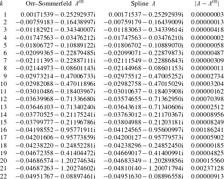
Appendix B. Solution of the
${\mathcal{H}}_{2}$
optimal control problem

This section presents the state-space formulas for the controller that solves the
 ${\mathcal{H}}_{2}$
optimal control problem. The reader is referred to Doyle et al. (Reference Doyle, Glover, Khargonekar and Francis1989) and Zhou et al. (Reference Zhou, Doyle and Glover1996, chap. 14) for the derivation of the formulas and more information about this control theory. The
 ${\mathcal{H}}_{2}$
control problem considers the generalised plant with state-space realisation
 $$\begin{eqnarray}\displaystyle \left.\begin{array}{@{}c@{}}\dot{\boldsymbol{u}}=\unicode[STIX]{x1D63C}\boldsymbol{u}+\unicode[STIX]{x1D63D}_{1}\boldsymbol{w}+\unicode[STIX]{x1D63D}_{2}\unicode[STIX]{x1D753},\\ \boldsymbol{z}=\unicode[STIX]{x1D63E}_{1}\boldsymbol{u}+\unicode[STIX]{x1D63F}_{12}\unicode[STIX]{x1D753},\\ \unicode[STIX]{x1D742}=\unicode[STIX]{x1D63E}_{2}\boldsymbol{u}+\unicode[STIX]{x1D63F}_{21}\boldsymbol{w}.\end{array}\right\} & & \displaystyle\end{eqnarray}$$
The output feedback
 $\unicode[STIX]{x1D753}(s)=\unicode[STIX]{x1D646}(s)\unicode[STIX]{x1D742}(s)$
must internally (exponentially) stabilise the system and minimise the
 ${\mathcal{H}}_{2}$
norm of the closed-loop map
 $\unicode[STIX]{x1D64F}_{zw}$
defined by (2.34). This problem has a unique solution provided that:
-
(i)
$(\unicode[STIX]{x1D63C},\unicode[STIX]{x1D63D}_{2},\unicode[STIX]{x1D63E}_{2})$
is stabilisable and detectable; -
(ii)
$\unicode[STIX]{x1D63F}_{12}$
and
$\unicode[STIX]{x1D63F}_{21}$
have full rank; -
(iii)
$\left[\!\begin{smallmatrix}\unicode[STIX]{x1D63C}-\text{i}\unicode[STIX]{x1D714}\unicode[STIX]{x1D644} & \unicode[STIX]{x1D63D}_{2}\\ \unicode[STIX]{x1D63E}_{1} & \unicode[STIX]{x1D63F}_{12}\end{smallmatrix}\!\right]$
has full column rank for all
$\unicode[STIX]{x1D714}$
; -
(iv)
$\left[\!\begin{smallmatrix}\unicode[STIX]{x1D63C}-\text{i}\unicode[STIX]{x1D714}\unicode[STIX]{x1D644} & \unicode[STIX]{x1D63D}_{1}\\ \unicode[STIX]{x1D63E}_{2} & \unicode[STIX]{x1D63F}_{21}\end{smallmatrix}\!\right]$
has full row rank for all
$\unicode[STIX]{x1D714}$
.


The state-space realisation of the optimal controller
 $\unicode[STIX]{x1D646}(s)$
is then given by
 $$\begin{eqnarray}\displaystyle \left.\begin{array}{@{}c@{}}\dot{\boldsymbol{u}}_{K}=\unicode[STIX]{x1D63C}_{K}\boldsymbol{u}_{K}+\unicode[STIX]{x1D63D}_{K}\unicode[STIX]{x1D742},\\ \unicode[STIX]{x1D753}=\unicode[STIX]{x1D63E}_{K}\boldsymbol{u}_{K},\end{array}\right\} & & \displaystyle\end{eqnarray}$$
where
 $$\begin{eqnarray}\displaystyle \left.\begin{array}{@{}c@{}}\unicode[STIX]{x1D63E}_{K}=-(\unicode[STIX]{x1D63D}_{2}^{\ast }\unicode[STIX]{x1D653}+\unicode[STIX]{x1D63F}_{12}^{\ast }\unicode[STIX]{x1D63E}_{1}),\\ \unicode[STIX]{x1D63D}_{K}=(\unicode[STIX]{x1D654}\unicode[STIX]{x1D63E}_{2}^{\ast }+\unicode[STIX]{x1D63D}_{1}\unicode[STIX]{x1D63F}_{21}^{\ast }),\\ \unicode[STIX]{x1D63C}_{K}=\unicode[STIX]{x1D63C}+\unicode[STIX]{x1D63D}_{2}\unicode[STIX]{x1D63E}_{K}-\unicode[STIX]{x1D63D}_{K}\unicode[STIX]{x1D63E}_{2},\end{array}\right\} & & \displaystyle\end{eqnarray}$$
and where
 $\unicode[STIX]{x1D653}$
and
 $\unicode[STIX]{x1D654}$
are the unique solution of the following algebraic Riccati equations
 $$\begin{eqnarray}\displaystyle \left.\begin{array}{@{}c@{}}(\unicode[STIX]{x1D63C}-\unicode[STIX]{x1D63D}_{2}\unicode[STIX]{x1D63F}_{12}^{\ast }\unicode[STIX]{x1D63E}_{1})^{\ast }\unicode[STIX]{x1D653}+\unicode[STIX]{x1D653}(\unicode[STIX]{x1D63C}-\unicode[STIX]{x1D63D}_{2}\unicode[STIX]{x1D63F}_{12}^{\ast }\unicode[STIX]{x1D63E}_{1})-\unicode[STIX]{x1D653}\unicode[STIX]{x1D63D}_{2}\unicode[STIX]{x1D63D}_{2}^{\ast }\unicode[STIX]{x1D653}+\unicode[STIX]{x1D63E}_{1}^{\ast }\unicode[STIX]{x1D63E}_{1}-\unicode[STIX]{x1D63E}_{1}^{\ast }\unicode[STIX]{x1D63F}_{12}\unicode[STIX]{x1D63F}_{12}^{\ast }\unicode[STIX]{x1D63E}_{1}=0,\\ (\unicode[STIX]{x1D63C}-\unicode[STIX]{x1D63D}_{1}\unicode[STIX]{x1D63F}_{21}^{\ast }\unicode[STIX]{x1D63E}_{2})\unicode[STIX]{x1D654}+\unicode[STIX]{x1D654}(\unicode[STIX]{x1D63C}-\unicode[STIX]{x1D63D}_{1}\unicode[STIX]{x1D63F}_{21}^{\ast }\unicode[STIX]{x1D63E}_{2})^{\ast }-\unicode[STIX]{x1D654}\unicode[STIX]{x1D63E}_{2}^{\ast }\unicode[STIX]{x1D63E}_{2}\unicode[STIX]{x1D654}+\unicode[STIX]{x1D63D}_{1}\unicode[STIX]{x1D63D}_{1}^{\ast }-\unicode[STIX]{x1D63D}_{1}\unicode[STIX]{x1D63F}_{21}^{\ast }\unicode[STIX]{x1D63F}_{21}\unicode[STIX]{x1D63D}_{1}^{\ast }=0.\end{array}\right\} & & \displaystyle\end{eqnarray}$$
For the control objective considered in this paper there are no cross-terms in the cost function
 $\boldsymbol{z}$
, that is
 $\unicode[STIX]{x1D63F}_{12}^{\ast }\unicode[STIX]{x1D63E}_{1}=0$
and the process noise and measurement noise are assumed to be uncorrelated, that is
 $\unicode[STIX]{x1D63D}_{1}\unicode[STIX]{x1D63F}_{21}^{\ast }=0$
.



