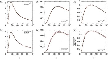
1 Introduction
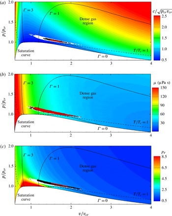
Turbulent flows of dense gases represent a research field of great importance for a wide range of applications in the fields of process engineering and energy conversion cycles. Dense gases are usually defined as single-phase fluids with complex heavy molecules, which operate in the vapour phase at pressures and temperatures of the order of magnitude of those of the liquid/vapour critical point. The dynamics of dense-gas flows is governed by the fundamental derivative of gas dynamics (Thompson Reference Thompson1971):
 $$\begin{eqnarray}\unicode[STIX]{x1D6E4}=1+\frac{\unicode[STIX]{x1D70C}}{c}\left(\frac{\unicode[STIX]{x2202}c}{\unicode[STIX]{x2202}\unicode[STIX]{x1D70C}}\right)_{s},\end{eqnarray}$$
where
 $\unicode[STIX]{x1D70C}$
is the fluid density,
 $c$
is the speed of sound and
 $s$
is the entropy, which measures relative variations of the speed of sound in isentropic transformations (Cramer & Kluwick Reference Cramer and Kluwick1984) and is directly related to the molecular complexity of the gas (Guardone & Argrow Reference Guardone and Argrow2005). It is usual to identify dense gases as fluids that exhibit values of
 $\unicode[STIX]{x1D6E4}$
lower than one in their vapour phase. In such conditions, the speed of sound tends to decrease in isentropic compressions and increase in expansions, contrary to the behaviour of lighter, ‘classical’ gases, like air or steam. The reversed variations of the speed of sound deeply modify the behaviour of dense-gas flows in the transonic and supersonic regime compared to more standard fluids. The most striking differences are expected for the so-called Bethe–Zel’dovich–Thompson (BZT) fluids, which exhibit a region of negative
 $\unicode[STIX]{x1D6E4}$
values in their vapour phase (inversion zone), leading to the appearance of non-classical phenomena like expansion shocks in some ranges of thermodynamic conditions (Cramer & Kluwick Reference Cramer and Kluwick1984). More details about the peculiar gas dynamics of dense gases and more specifically of BZT fluids can be found in Cinnella & Congedo (Reference Cinnella and Congedo2007).
Despite the increasing interest in using dense gases in applications, such as organic Rankine cycles (ORC) (see, e.g. Monaco, Cramer & Watson Reference Monaco, Cramer and Watson1997; Brown & Argrow Reference Brown and Argrow2000; Congedo, Corre & Cinnella Reference Congedo, Corre and Cinnella2011), the influence of dense-gas effects on turbulence remains unexplored because experimental measurements are very difficult. In particular, understanding and modelling high-speed flow effects is of utmost importance for the design and performance analysis of supersonic ORC turbine expanders (Bufi & Cinnella Reference Bufi and Cinnella2015). The dynamics of compressible turbulence in the presence of strong dense-gas effects was first investigated in Sciacovelli et al. (Reference Sciacovelli, Cinnella, Content and Grasso2016a ). In this work, Euler-based numerical simulations were used to study the large-scale dynamics of compressible homogeneous isotropic turbulence (HIT) of a BZT gas, for which expansion shocks may occur at particular thermodynamic conditions in the transonic and supersonic flow regions. At sufficiently high turbulent Mach number, compressible HIT is significantly modified by dense-gas effects. Specifically, it was observed that the reversed speed of sound behaviour leads to large density and speed of sound fluctuations despite negligible temperature fluctuations, and to much more symmetric probability distribution functions, e.g. of the local dilatation, due to the weakening of compressive structures and the enhancement of expansion ones. For the dense-gas, strong expansion regions are characterized by sheet-like structures, unlike the perfect gas which exhibits tubular structures. Moreover, expansion eddy shocklets may appear in the dense gas. Additionally, viscous studies were carried out to elucidate dense-gas effects on the small-scale dynamics (Sciacovelli & Cinnella Reference Sciacovelli and Cinnella2015; Sciacovelli, Cinnella & Grasso Reference Sciacovelli, Cinnella and Grasso2016b ). Strong expansion regions are found to contribute to the dilatational dissipation by an amount comparable to compression regions. This is due to the occurrence of steep expanding structures and possibly of expansion shocklets which contribute to enstrophy generation and counterbalance enstrophy destruction introduced by eddy-like structures.
Wall turbulence includes several phenomena that are absent in HIT, such as the mean shear or variations of mean density. A peculiar feature in the dense-gas regime is that the dynamic viscosity
 $\unicode[STIX]{x1D707}$
and the thermal conductivity
 $\unicode[STIX]{x1D705}$
depend both on temperature and pressure through complex relationships. Consequently, a dense gas can exhibit both gas-like behaviour, with strong compressibility effects due to the non-standard variations of its sound speed, and liquid-like features with a viscosity decreasing as the temperature increases. We also stress here that, differently from perfect gases, the transport properties of dense gases also depend on density (or pressure) and not on temperature only. This dependency also represents a major difference with respect to variable-property liquids, whose density and viscosity depend on the temperature only. Note that the heat capacity
 $c_{p}$
of a dense gas is generally much larger than the one of a classical gas, implying a weaker coupling between the dynamic and thermal boundary layers, so that isothermal transformations are also almost adiabatic. Even for supersonic flows, characterized by high values of the Mach number, friction heating is expected to be reduced, leading to small temperature variations, like in the incompressible flow limit. The overall behaviour is nonetheless unforeseen due for instance to strong variations of Prandtl number
 $Pr$
in regions where
 $c_{p}$
becomes large. In summary, the peculiar variations of the thermodynamic and transport properties in dense gases are expected to alter the conventional behaviour of turbulence via complex nonlinear couplings.
The coupling between turbulence and state variables is a problem of fundamental interest and has been discussed notably for high-speed flows, where compressibility effects come into play, or in the context of strong variations of properties where the temperature can no longer be considered as a passive scalar.
The question of the effects of compressibility on the structure of wall-bounded turbulence is tightly related to variations of the density, temperature, viscosity and thermal conductivity, leading to variations of the Reynolds and Mach numbers across the flow. Chu & Kovasznay (Reference Chu and Kovasznay1958) proposed a general decomposition into vorticity, acoustic and entropic modes and analysed systematically their interactions up to the second order. The effects of variable transport properties on heat transfer or large-scale coherent structures can then be viewed as interactions between vorticity and entropy modes. For supersonic wall-bounded flows, the main lesson learned from previous studies is that the vortical motions are weakly affected by variations of mean properties and the large-scale organization of wall turbulence remains close to the one that has been extensively described for incompressible wall-bounded turbulence (Spina, Smits & Robinson Reference Spina, Smits and Robinson1994). The nonlinear coupling with acoustic or entropy modes (Chu & Kovasznay Reference Chu and Kovasznay1958) does not generate substantial sources of the vorticity mode. This passive character of compressible wall turbulence is well summarized by Morkovin’s hypothesis (Morkovin Reference Morkovin and Favre1961), i.e. that compressibility mainly influences the turbulence through variations in mean density, whereas the density fluctuations have a negligible effect. Compressibility mainly modulates the turbulence through variations in the mean values of thermodynamic quantities. Since the flow dynamics essentially follows an incompressible pattern, a lot of studies have focused on the incompressible–compressible correspondence. Indeed, since no universal theory for wall-bounded compressible flows is available so far, the incompressible limit remains an interesting reference to quantify the alteration of turbulence structure. In particular, efforts have been made to extend conventional scaling laws for constant property flows to compressible conditions (Bradshaw Reference Bradshaw1977).
Understanding how the peculiar variations of the thermodynamic and transport properties typical of dense gases influence the behaviour of wall-bounded turbulent flows is of primal importance for providing a correct description of friction drag and heat fluxes in many applications, and to develop suitable models for predicting them. Measurements of dense-gas flows are hardly available due to the difficulty of conducting measurements of this kind of flows. Furthermore, most of the facilities presently under development are thought to provide average pressure and temperature profiles and, in some cases, flow visualizations, but are not expected to provide a detailed description of the turbulence structure, at least in the short term. A review of recent experimental research on dense-gas flows can be found in Spinelli et al. (Reference Spinelli, Pini, Dossena, Gaetani and Casella2013) and Mathijssen et al. (Reference Mathijssen, Gallo, Casati, Nannan, Zamfirescu, Guardone and Colonna2015). For these reasons, in this work we choose to investigate wall-bounded turbulent dense-gas flows by means of direct numerical simulations (DNS) of the Navier–Stokes equations, supplemented by suitable thermodynamic and transport property models. More specifically, we conduct parametric numerical experiments for the compressible turbulent channel flow. This configuration is well suited for a systematic study of wall-bounded turbulence without complicating features such as streamwise development, shocks or separation.
The first DNS of compressible turbulent channel flow of a perfect gas have been performed by Coleman, Kim & Moser (Reference Coleman, Kim and Moser1995) and Huang, Coleman & Bradshaw (Reference Huang, Coleman and Bradshaw1995). They considered a plane channel flow between two (cooled) isothermal walls for two values of the bulk Mach number, namely 1.5 and 3, and two values of the Reynolds number based on bulk quantities and wall viscosity (3000 and 4880, respectively). They found that the flow is influenced by the strong wall-normal gradients of the mean density. One of the main results was the confirmation of the validity of the Morkovin hypothesis. Data were further analysed by Huang et al. (Reference Huang, Coleman and Bradshaw1995) who introduced a semi-local scaling where local thermodynamic properties for density and viscosity replaces wall values to collapse turbulent statistics. The agreement with incompressible data is improved for mean streamwise velocity profiles compared to the Van Driest transformation (Van Driest Reference Van Driest1951) often used for turbulent boundary layers with adiabatic walls. Lechner, Sesterhenn & Friedrich (Reference Lechner, Sesterhenn and Friedrich2001) reproduced the DNS of Coleman et al. (Reference Coleman, Kim and Moser1995) at
 $M=1.5$
and
 $Re=3000$
and studied scatter plots to analyse sweeps and ejections in the wall layer. They reported a slight change in Reynolds stresses anisotropy compared to the incompressible case. Foysi, Sarkar & Friedrich (Reference Foysi, Sarkar and Friedrich2004) investigated turbulent channel flow with isothermal walls using DNS with Mach numbers up to 3.5 and Reynolds numbers based on friction velocity (
 $Re_{\unicode[STIX]{x1D70F}}$
) up to 1030. They focused on the behaviour of pressure fluctuations and also found that turbulent stresses are mainly affected by mean property variation so that the semi-local scaling is well suited for comparison with incompressible cases. Morinishi, Tamano & Nakabayashi (Reference Morinishi, Tamano and Nakabayashi2004) complemented the study of Coleman et al. (Reference Coleman, Kim and Moser1995) by investigating the influence of the thermal condition at the wall. They performed DNS of compressible channel flows between both adiabatic and isothermal walls at Mach number 1.5. Tamano & Morinishi (Reference Tamano and Morinishi2006) considered the asymmetric case of a channel with a cold and a hot wall, either adiabatic or isothermal. Heat transfers can reduce compressibility effects but remain of limited importance, and the Morkovin hypothesis is still applicable. Brun et al. (Reference Brun, Boiarciuc, Hakerborn and Comte2008) performed large-eddy simulations of fully developed channel flows with specific focus on wall modelling. They proposed a variant of the semi-local scaling for both amplitude and distance and arrive at the same conclusions as Huang et al. (Reference Huang, Coleman and Bradshaw1995) or Morinishi et al. (Reference Morinishi, Tamano and Nakabayashi2004). Wei & Pollard (Reference Wei and Pollard2011) studied the influence of the Mach number,
 $M=0.2$
, 0.7 and 1.5, at constant bulk Reynolds number and proposed budgets of transport properties. Gerolymos & Vallet (Reference Gerolymos and Vallet2014) performed a series of DNS and derived transport equations to study in detail the variance of thermodynamic fluctuations. Trettel & Larsson (Reference Trettel and Larsson2016) gave a theoretical framework to the semi-local scaling of Huang et al. (Reference Huang, Coleman and Bradshaw1995) showing that the scaling of the wall distance is important to take into account the variable mean properties. A good match with incompressible distributions is found for a wide range of Reynolds and Mach numbers. Recently, Modesti & Pirozzoli (Reference Modesti and Pirozzoli2016) produced an extensive DNS database increasing the bulk Reynolds number up to
 $Re=34\,000$
. They applied the different scalings proposed in previous studies and showed that the transformation of Trettel & Larsson (Reference Trettel and Larsson2016) very well reproduces the behaviour of the mean velocity profile by matching the friction Reynolds number based on semi-local quantities.
In terms of coherent motions in the wall layer, Coleman et al. (Reference Coleman, Kim and Moser1995) identified an enhanced coherence of near-wall streaks when compared to the incompressible references. Greater streak elongation was also reported for supersonic boundary layers with cooled walls, whereas a tendency towards shorter streaks is noted for heated walls (Duan, Beekman & Martin Reference Duan, Beekman and Martin2010; Lagha et al. Reference Lagha, Kim, Eldredge and Zhong2011). Morinishi et al. (Reference Morinishi, Tamano and Nakabayashi2004) noted that streaks do not become more coherent if the semi-local scaling is used instead of wall units to non-dimensionalize the lengths. This was confirmed later by Patel et al. (Reference Patel, Peeters, Boersma and Pecnik2015) for low Mach number flows with variable properties.
Given the importance of mean density and viscosity variations, other studies have considered turbulent channel flow with variable properties without compressibility effects due to high speed. Some studies have investigated heat transfers in turbulent channel flow by treating temperature as a passive scalar. For instance, Teitel & Antonia (Reference Teitel and Antonia1993) considered the influence of different thermal wall conditions and noted the importance of the value of the Prandtl number for heat transfers. Nicoud & Poinsot (Reference Nicoud and Poinsot1999) investigated by DNS the effects of variable density and molecular viscosity on a channel flow between two isothermal walls for different temperature ratios or viscosity laws. Low Mach simulations are used and support Van Driest scaling for mean velocity profiles and semi-local scaling for Reynolds stresses. Several works have investigated the effects of temperature-dependent properties using a nonlinear coupling algorithm (Bae, Yoo & Choi Reference Bae, Yoo and Choi2005; Li et al.
Reference Li, Hashimoto, Tominaga, Tanahashi and Miyauchi2008; Sewall & Tafti Reference Sewall and Tafti2008; Zonta, Marchioli & Soldati Reference Zonta, Marchioli and Soldati2012). In all of these studies the viscosity, density and thermal conductivity vary with the temperature. Zonta et al. (Reference Zonta, Marchioli and Soldati2012) considered temperature gradients in water channel flow and examined the turbulent kinetic energy budgets. Lee et al. (Reference Lee, Jung, Sung and Zaki2013) showed that the viscosity stratification and associated wall heating can alter the ejections and sweeps events in an incompressible turbulent boundary layer. Bae et al. (Reference Bae, Yoo and Choi2005) studied the turbulent heat transfer mechanisms of supercritical carbon dioxide (
 $\text{CO}_{2}$
) performing DNS in heated vertical tubes. They focused on the well-known heat transfer deterioration phenomenon in supercritical flows. Li et al. (Reference Li, Hashimoto, Tominaga, Tanahashi and Miyauchi2008) investigated the same fluid in a long plane channel by imposing wall temperature variations in the streamwise direction, i.e. considering heating and cooling regions at the beginning and at the end of the channel, respectively. They found that the effects of density fluctuations, particularly near the pseudo-critical temperature, on turbulent kinetic energy cannot be ignored, and that the different temperature values cause a modulation of the near-wall turbulent structures. Patel et al. (Reference Patel, Peeters, Boersma and Pecnik2015) conducted numerical experiments by imposing different distributions for the fluid properties to investigate separately the effects of mean density or viscosity gradients in low Mach number turbulent channel flow. They showed that various laws bearing similarities either with liquid-like or gas-like behaviour can be taken into account for turbulent statistics by using the semi-local scaling introduced in the compressible regime. In particular, a good similarity was observed for an equivalent friction Reynolds number constructed with semi-local quantities.
To the authors’ knowledge, compressible wall-bounded flows have been almost exclusively investigated for air, modelled as a perfect polytropic gas. A few studies have considered variable-property or supercritical fluids with a low Mach number assumption. In this work, we present new direct numerical simulations of compressible turbulent channel flows for PP11, a heavy fluorocarbon representative of dense gases. The thermodynamic and transport property behaviour of the fluid are described by means of advanced models. A parametric study for different bulk Mach and Reynolds numbers is conducted and the results are compared with perfect-gas flows (air flows) at the same bulk conditions. The present paper is organized as follows. The governing equations and numerical set-up are provided in § 2. The present DNS data and global characteristics are presented in § 3. In § 4, the effects of dense-gas flows on mean and fluctuating properties are explained. In § 5, the profile of turbulence intensities, turbulent kinetic budgets and near-wall structures are investigated. The analysis is performed by comparing with the flows for an ideal gas. Validation test cases and details about the transport properties laws for dense gases are given in the appendices.
2 Methodology
2.1 Governing equations
In the present study we consider flows of gases in the single-phase regime, governed by the compressible Navier–Stokes equations, written in differential form as
 $$\begin{eqnarray}\displaystyle & \displaystyle \frac{\unicode[STIX]{x2202}\unicode[STIX]{x1D70C}}{\unicode[STIX]{x2202}t}+\frac{\unicode[STIX]{x2202}(\unicode[STIX]{x1D70C}u_{j})}{\unicode[STIX]{x2202}x_{j}}=0 & \displaystyle\end{eqnarray}$$
 $$\begin{eqnarray}\displaystyle & \displaystyle \frac{\unicode[STIX]{x2202}(\unicode[STIX]{x1D70C}u_{i})}{\unicode[STIX]{x2202}t}+\frac{\unicode[STIX]{x2202}(\unicode[STIX]{x1D70C}u_{i}u_{j})}{\unicode[STIX]{x2202}x_{j}}+\frac{\unicode[STIX]{x2202}p}{\unicode[STIX]{x2202}x_{i}}-\frac{\unicode[STIX]{x2202}\unicode[STIX]{x1D70F}_{ij}}{\unicode[STIX]{x2202}x_{j}}=\unicode[STIX]{x1D70C}f_{u_{i}} & \displaystyle\end{eqnarray}$$
 $$\begin{eqnarray}\displaystyle & \displaystyle \frac{\unicode[STIX]{x2202}(\unicode[STIX]{x1D70C}E)}{\unicode[STIX]{x2202}t}+\frac{\unicode[STIX]{x2202}((\unicode[STIX]{x1D70C}E+p)u_{j})}{\unicode[STIX]{x2202}x_{j}}-\frac{\unicode[STIX]{x2202}(\unicode[STIX]{x1D70F}_{ij}u_{i})}{\unicode[STIX]{x2202}x_{j}}+\frac{\unicode[STIX]{x2202}q_{j}}{\unicode[STIX]{x2202}x_{j}}=\unicode[STIX]{x1D70C}f_{u_{i}}u_{i}, & \displaystyle\end{eqnarray}$$
where
 $u_{i}$
is the velocity vector,
 $\unicode[STIX]{x1D70C}$
the density and
 $p$
the pressure. The specific total energy
 $E$
and the viscous stress tensor
 $\unicode[STIX]{x1D70F}_{ij}$
are defined as
 $$\begin{eqnarray}\displaystyle & \displaystyle E\equiv e+{\textstyle \frac{1}{2}}u_{j}^{2} & \displaystyle\end{eqnarray}$$
 $$\begin{eqnarray}\displaystyle & \displaystyle \unicode[STIX]{x1D70F}_{ij}\equiv 2\unicode[STIX]{x1D707}\unicode[STIX]{x1D61A}_{ij}+\unicode[STIX]{x1D706}\unicode[STIX]{x1D703}\unicode[STIX]{x1D6FF}_{ij}, & \displaystyle\end{eqnarray}$$
where
 $e$
is the specific internal energy,
 $\unicode[STIX]{x1D707}$
the dynamic viscosity,
 $\unicode[STIX]{x1D61A}_{ij}=(1/2)((\unicode[STIX]{x2202}u_{i}/\unicode[STIX]{x2202}x_{j})+(\unicode[STIX]{x2202}u_{j}/\unicode[STIX]{x2202}x_{i}))$
is the strain rate tensor,
 $\unicode[STIX]{x1D703}\equiv \unicode[STIX]{x2202}u_{k}/\unicode[STIX]{x2202}x_{k}$
the velocity divergence or dilatation,
 $\unicode[STIX]{x1D6FF}_{ij}$
the Kronecker symbol and
 $\unicode[STIX]{x1D706}=-2\unicode[STIX]{x1D707}/3$
the second viscosity according to Stokes’ hypothesis. Finally,
 $q_{j}$
represents the heat flux, modelled by means of the Fourier’s law:
 $$\begin{eqnarray}q_{j}=-\unicode[STIX]{x1D705}\frac{\unicode[STIX]{x2202}T}{\unicode[STIX]{x2202}x_{j}},\end{eqnarray}$$
where
 $\unicode[STIX]{x1D705}$
is the thermal conductivity. The system is supplemented by thermal and caloric equations of state, respectively:
 $$\begin{eqnarray}p=p(\unicode[STIX]{x1D70C},T)\quad \text{and}\quad e=e(\unicode[STIX]{x1D70C},T).\end{eqnarray}$$
These variables satisfy the compatibility relation:
 $$\begin{eqnarray}e=e_{r}+\int _{T_{r}}^{T}c_{v,\infty }(T^{\prime })\,\text{d}T^{\prime }-\int _{\unicode[STIX]{x1D70C}_{r}}^{\unicode[STIX]{x1D70C}}\left[T\left.\frac{\unicode[STIX]{x2202}p}{\unicode[STIX]{x2202}T}\right|_{\unicode[STIX]{x1D70C}}-p\right]\frac{\text{d}\unicode[STIX]{x1D70C}^{\prime }}{\unicode[STIX]{x1D70C}^{\prime 2}},\end{eqnarray}$$
where the subscript
 $(\cdot )_{r}$
indicates a reference state,
 $c_{v,\infty }(T)$
is the specific heat at constant volume in the ideal-gas limit, and the superscript
 $(\cdot )^{\prime }$
denotes auxiliary integration variables. For a thermally and calorically perfect gas, equations (2.7) become:
 $$\begin{eqnarray}p=\unicode[STIX]{x1D70C}RT\quad \text{and}\quad e=c_{v}T,\end{eqnarray}$$
where
 $c_{v}=R/(\unicode[STIX]{x1D6FE}-1)=\text{const.}$
, and
 $R={\mathcal{R}}$
with
 ${\mathcal{R}}$
the universal gas constant and
 ${\mathcal{M}}$
the gas molecular weight. Moreover, thermodynamic models relating the dynamic viscosity
 $\unicode[STIX]{x1D707}$
and thermal conductivity
 $\unicode[STIX]{x1D705}$
to the gas temperature and pressure are needed. In the following simulations, we consider the perfluoro-perhydrophenanthrene, (chemical formula
 $\text{C}_{14}\text{F}_{24}$
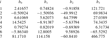
), called hereafter PP11 (commercial name), whose thermodynamic properties are provided in table 1 (see Cramer Reference Cramer1989). This fluid has been often used in the literature since it exhibits a wide inversion zone and thus significant dense-gas effects. The thermodynamic behaviour of the fluid is modelled through the Martin–Hou thermal equation of state (Martin & Hou Reference Martin and Hou1955), which provides a reasonably accurate description of the gas behaviour and of the inversion zone size. Such an equation involves five virial terms and ensures high accuracy with a minimum amount of experimental information. The equation reads:
 $$\begin{eqnarray}p=\frac{RT}{(v-b)}+\mathop{\sum }_{i=2}^{5}\frac{f_{i}(T)}{(v-b)^{i}},\end{eqnarray}$$
with
 $b=v_{cr}(1-\unicode[STIX]{x1D6FD}/Z_{cr})$
,
 $\unicode[STIX]{x1D6FD}=20.533Z_{cr}-31.883Z_{cr}^{2}$
, and
 $$\begin{eqnarray}f_{i}(T)=A_{i}+B_{i}T+C_{i}\exp (-kT/T_{cr}),\end{eqnarray}$$
where
 $v=1/\unicode[STIX]{x1D70C}$
denotes the specific volume,
 $v_{cr}$
,
 $T_{cr}$
and
 $Z_{cr}$
the critical specific volume, temperature and compressibility factor, respectively, and
 $k=5.475$
.
 $A_{i}$
,
 $B_{i}$
and
 $C_{i}$
are gas-dependent coefficients that can be expressed in terms of the critical temperature and pressure, the critical compressibility factor, the Boyle temperature (which may be expressed as a function of the critical temperature) and one point on the vapour pressure curve. A power law of the form:
 $$\begin{eqnarray}c_{v_{\infty }}(T)=c_{v_{\infty }}(T_{cr})\left(\frac{T}{T_{cr}}\right)^{n}\end{eqnarray}$$
is used to model variations of the low-density specific heat with temperature, where
 $n$
is a material-dependent parameter. The fluid viscosity and thermal conductivity are evaluated by means of the generalized laws derived by Chung et al. (Reference Chung, Ajlan, Lee and Starling1988), which contain a correction term that takes into account the strong density dependence of the transport properties in the dense-gas region. These laws, extensively used in previous works (Cramer & Tarkenton Reference Cramer and Tarkenton1992; Cramer & Park Reference Cramer and Park1999), are described in appendix A. In the modelling, the bulk viscosity
 $\unicode[STIX]{x1D707}_{b}=\unicode[STIX]{x1D706}+2\unicode[STIX]{x1D707}/3$
is set to zero, assuming a Stokesian fluid. Since this coefficient is multiplied by the divergence of the velocity
 $\unicode[STIX]{x1D703}$
, the hypothesis is exact in the incompressible limit. This is also a very good approximation for low Mach numbers, for monoatomic gases, but can be questioned for a complex molecular fluid (Cramer & Bahmani Reference Cramer and Bahmani2014). The study of Cramer (Reference Cramer2012) provides some numerical estimates for the bulk viscosity of ideal gases. It shows that the latter can vary significantly with the temperature and can be as large as hundreds or thousands of times the shear viscosity, even for some common diatomic gases. Interestingly, the bulk viscosity ratio
 $\unicode[STIX]{x1D707}_{b}/\unicode[STIX]{x1D707}$
is a decreasing function of the temperature for most gases, except, e.g. methane (
 $\text{CH}_{4}$
) which exhibits a peak around
 $T\approx 400~\text{K}$
(
 $\unicode[STIX]{x1D707}_{b}/\unicode[STIX]{x1D707}\approx 350$
). Specifically, for the fluorocarbon SF
 $_{6}$
, commonly considered as a dense gas (Anderson Reference Anderson1991),
 $\unicode[STIX]{x1D707}_{b}/\unicode[STIX]{x1D707}$
decreases quickly with
 $T$
, dropping from approximately 300 at 300 K to less than 50 at temperatures between 600 and 700 K, like the ones of interest in the present study. Even if the value of
 $\unicode[STIX]{x1D707}_{b}$
is unknown for a dense gas such as PP11, the effect of the bulk viscosity has been tested by taking a large value
 $\unicode[STIX]{x1D707}_{b}=500\unicode[STIX]{x1D707}$
. The results are almost unaffected (see appendix B) so that Stokes hypothesis (
 $\unicode[STIX]{x1D707}_{b}=0$
) is retained in the following.
Thermodynamic properties of PP11: molecular weight (
 ${\mathcal{M}}$
), critical temperature (
 $T_{cr}$
), critical density (
 $\unicode[STIX]{x1D70C}_{cr}$
), critical pressure (
 $p_{cr}$
), critical compressibility factor (
 $Z_{cr}$
), acentric factor (
 $\unicode[STIX]{x1D714}$
), dipole moment of the gas phase (
 $\unicode[STIX]{x1D709}$
), boiling temperature (
 $T_{b}$
) and ratio of ideal-gas specific heat at constant volume over the gas constant (
 $c_{v}(T_{cr})/R$
) at the critical point.

2.2 Numerical methods
Calculations are based on an in-house computational fluid dynamics (CFD) code (Gloerfelt & Berland Reference Gloerfelt and Berland2013) equipped with high-order dispersion relation preserving schemes. The convective flux derivatives are approximated by using a fourth-order optimized finite-difference scheme on an eleven-point stencil, described in Bogey & Bailly (Reference Bogey and Bailly2004), while standard fourth-order finite differences are used to discretize the viscous fluxes. Non-uniform mesh sizes are taken into account by means of coordinate transforms. To ensure accuracy, mesh stretching rate is kept below 1.5 %. As a part of the algorithm, the optimized selective sixth-order filter of Bogey, De Cacqueray & Bailly (Reference Bogey, De Cacqueray and Bailly2009) is applied in each direction in order to eliminate grid-to-grid unresolved oscillations. Finally, time integration is carried out by means of a low-storage six-step Runge–Kutta scheme optimized in the wavenumber space (Bogey & Bailly Reference Bogey and Bailly2004).
The numerical strategy has been widely employed for jets (Bogey & Bailly Reference Bogey and Bailly2009; Bogey, Marsden & Bailly Reference Bogey, Marsden and Bailly2012) as well as turbulent boundary layers (Aubard, Gloerfelt & Robinet Reference Aubard, Gloerfelt and Robinet2013; Gloerfelt & Berland Reference Gloerfelt and Berland2013). The code has been preliminarily validated for turbulent channel flow configurations by comparison with reference results for both subsonic (Kim, Moin & Moser Reference Kim, Moin and Moser1987) and supersonic (Coleman et al. Reference Coleman, Kim and Moser1995) channel flows of a perfect gas (see appendix C).
3 Numerical experiments of compressible channel flows
3.1 Set-up and definitions
Numerical experiments are conducted for the plane channel flow configuration, i.e. the flow between two infinite parallel flat plates. This is reproduced by applying periodic conditions in the homogeneous streamwise (
 $x$
) and spanwise (
 $z$
) directions. Isothermal no-slip wall conditions are applied on the lower and upper walls. In order to counteract viscous friction and maintain a target bulk mass flow, the approach described in Gerolymos, Sénéchal & Vallet (Reference Gerolymos, Sénéchal and Vallet2010) and Gerolymos & Vallet (Reference Gerolymos and Vallet2014) is used to compute the forcing term. Specifically, at the end of each Runge–Kutta stage, the bulk density is explicitly constrained to maintain a fixed target value, whereas a source term
 $f_{u_{1}}$
is injected in the streamwise momentum equation to enforce a constant mass flow. It should be noted that the density correction is equivalent to including a source term in the continuity equation. Nevertheless, this term is very small and can be neglected (Coleman et al.
Reference Coleman, Kim and Moser1995; Huang et al.
Reference Huang, Coleman and Bradshaw1995; Lechner et al.
Reference Lechner, Sesterhenn and Friedrich2001; Foysi et al.
Reference Foysi, Sarkar and Friedrich2004; Morinishi et al.
Reference Morinishi, Tamano and Nakabayashi2004; Wei & Pollard Reference Wei and Pollard2011; Gerolymos & Vallet Reference Gerolymos and Vallet2014).
In the following, the subscripts
 $(\cdot )_{B}$
,
 $(\cdot )_{w}$
and
 $(\cdot )_{c}$
denote averaging over the whole computational domain, the walls and centreline, respectively;
 $\overline{(\cdot )}$
indicates Reynolds averaging and
 $(\cdot )^{\prime }$
are Reynolds fluctuations; similarly,
 $\widetilde{(\cdot )}$
and
 $(\cdot )^{\prime \prime }$
denote Favre averaging and Favre fluctuations. In the following, we also use the centreline Reynolds and Mach numbers, respectively defined as
 $Re_{c}=\overline{\unicode[STIX]{x1D70C}}_{c}\overline{u}_{c}h/\overline{\unicode[STIX]{x1D707}}_{c}$
and
 $\overline{M}_{c}=\overline{u_{c}/c_{c}}$
.
The DNS operating point is defined by a bulk Reynolds number
 $Re_{B}$
and a bulk Mach number
 $M_{B}$
, defined as:
 $$\begin{eqnarray}Re_{B}=\frac{\unicode[STIX]{x1D70C}_{B}\widetilde{u}_{B}h}{\overline{\unicode[STIX]{x1D707}}_{w}},\quad M_{B}=\frac{\widetilde{u}_{B}}{\overline{c}_{w}},\end{eqnarray}$$
where
 $\unicode[STIX]{x1D70C}_{B}$
is the bulk density,
 $\overline{\unicode[STIX]{x1D707}}_{w}$
is the dynamic viscosity and
 $\overline{c}_{w}$
the sound speed at the walls. In the definition of the bulk reference numbers, wall values for viscosity and speed of sound are usually considered since this greatly simplifies the imposition of the reference conditions for isothermal walls. Indeed, for a perfect-gas model, a fixed wall temperature implies
 $\overline{\unicode[STIX]{x1D707}}_{w}=\unicode[STIX]{x1D707}(T_{w})$
and
 $\overline{c}_{w}=c(T_{w})=\sqrt{\unicode[STIX]{x1D6FE}RT_{w}}$
. However, this is no longer true when using more complex thermodynamic models, since the speed of sound and the transport properties depend on both temperature and density values. In these cases,
 $\overline{\unicode[STIX]{x1D70C}}_{w}$
is not known a priori and it is not possible to fix directly
 $Re_{B}$
and
 $M_{B}$
. To enforce the reference conditions, an iterative procedure has been followed: first, a preliminary calculation is run by choosing a reasonable value for the ratio
 $\overline{\unicode[STIX]{x1D70C}}_{w}/\unicode[STIX]{x1D70C}_{B}$
. Once the solution is converged, the
 $\overline{\unicode[STIX]{x1D70C}}_{w}$
obtained from the simulation is used to compute the updated values of
 $\overline{\unicode[STIX]{x1D707}}_{w}$
and
 $\overline{c}_{w}$
, and the flow field is interpolated onto a new grid (adapted to the updated value of the Reynolds number). In order to achieve convergence to the desired state, about three to four iterative cycles are needed.
We recall the definition of the standard wall coordinates and friction Reynolds number
 $$\begin{eqnarray}y^{+}=\frac{\overline{\unicode[STIX]{x1D70C}}_{w}u_{\unicode[STIX]{x1D70F}}(y-y_{w})}{\overline{\unicode[STIX]{x1D707}}_{w}};\quad Re_{\unicode[STIX]{x1D70F}_{w}}=\frac{\overline{\unicode[STIX]{x1D70C}}_{w}u_{\unicode[STIX]{x1D70F}}h}{\overline{\unicode[STIX]{x1D707}}_{w}},\end{eqnarray}$$
where
 $u_{\unicode[STIX]{x1D70F}}=\sqrt{\unicode[STIX]{x1D70F}_{w}/\overline{\unicode[STIX]{x1D70C}}_{w}}$
is the friction velocity,
 $\unicode[STIX]{x1D70F}_{w}=\overline{(\unicode[STIX]{x1D707}(\unicode[STIX]{x2202}u/\unicode[STIX]{x2202}y))}_{w}$
being the shear stress at the wall. It is widely known that the Reynolds number based on the friction velocity does not correctly represent the effect of rapid wall-normal variations for density and viscosity profiles in presence of high compressibility effects. Huang et al. (Reference Huang, Coleman and Bradshaw1995) proposed an empirical semi-local scaling based on both wall and local mean quantities:
 $$\begin{eqnarray}y^{\ast }=\frac{\overline{\unicode[STIX]{x1D70C}}(y)u_{\unicode[STIX]{x1D70F}}^{\ast }(y-y_{w})}{\overline{\unicode[STIX]{x1D707}}(y)};\quad Re_{\unicode[STIX]{x1D70F}}^{\ast }(y)=Re_{\unicode[STIX]{x1D70F}_{w}}\sqrt{\frac{\overline{\unicode[STIX]{x1D70C}}(y)}{\overline{\unicode[STIX]{x1D70C}}_{w}}}\frac{\overline{\unicode[STIX]{x1D707}}_{w}}{\overline{\unicode[STIX]{x1D707}}(y)},\end{eqnarray}$$
with
 $u_{\unicode[STIX]{x1D70F}}^{\ast }=\sqrt{\unicode[STIX]{x1D70F}_{w}/\overline{\unicode[STIX]{x1D70C}}(y)}$
the semi-local friction velocity. This mixed scaling has proven to give quite satisfactory results in collapsing first- and second-order moments (Foysi et al.
Reference Foysi, Sarkar and Friedrich2004; Morinishi et al.
Reference Morinishi, Tamano and Nakabayashi2004; Modesti & Pirozzoli Reference Modesti and Pirozzoli2016) obtained from a wide range of
 $M_{B}$
and
 $Re_{B}$
. Recently, Patel et al. (Reference Patel, Peeters, Boersma and Pecnik2015) and Trettel & Larsson (Reference Trettel and Larsson2016) have developed a mathematical framework giving a theoretical basis to the semi-local scaling. Even if this scaling was initially introduced in order to take into account the effects of compressibility, Patel et al. (Reference Patel, Peeters, Boersma and Pecnik2015) assessed its validity also for variable-property flows, since it inherently considers the evolution of transport properties and their relation with thermodynamic quantities.
3.2 Description of the computed cases
Dense-gas effects are evaluated by means of a parametric study at three bulk Reynolds numbers (namely,
 $Re_{B}=3000$
, 7000 and 12 000) and three bulk Mach numbers (
 $M_{B}=1.5$
, 2.25 and 3.0). For PP11 cases, the bulk density was imposed to be
 $\unicode[STIX]{x1D70C}_{B}=0.618\unicode[STIX]{x1D70C}_{cr}$
and the wall temperature was fixed to
 $T_{w}=1.01T_{cr}$
. The density value ensures that the flow evolves in the dense-gas region, whereas the slightly supercritical wall temperature condition avoids the occurrence of a two-phase flow. It should be noted that for these conditions it is not possible to obtain negative values of the derivative of gas dynamics
 $\unicode[STIX]{x1D6E4}$
, so we should not expect BZT phenomena.
In the following, we refer to each simulation with a unique tag of the form
 $\text{XM}\unicode[STIX]{x1D6FC}\text{R}\unicode[STIX]{x1D6FD}$
, where the first letter indicates the fluid (A for air and P for PP11),
 $\unicode[STIX]{x1D6FC}$
refers to
 $M_{B}$
(
 $\unicode[STIX]{x1D6FC}=1,2,3$
for
 $M_{B}=1.5,2.25,3$
, respectively) and
 $\unicode[STIX]{x1D6FD}$
to
 $Re_{B}$
(
 $\unicode[STIX]{x1D6FD}=3,7,12$
for
 $Re_{B}=3000,7000,12\,000$
, respectively). For all the cases, the computational domain has dimensions
 $L_{x}\times L_{y}\times L_{z}=8\unicode[STIX]{x03C0}h\times 2h\times 2\unicode[STIX]{x03C0}h$
, with
 $h$
the channel half-height. Note that the dimension in the streamwise direction is greater than the one used in the previous compressible channel DNS (Coleman et al.
Reference Coleman, Kim and Moser1995; Lechner et al.
Reference Lechner, Sesterhenn and Friedrich2001; Morinishi et al.
Reference Morinishi, Tamano and Nakabayashi2004; Wei & Pollard Reference Wei and Pollard2011) in order to ensure uncorrelated inlet and outlet quantities for high-
 $M_{B}$
cases. The computational grids are chosen in order to provide a good spatial resolution in all directions. Specifically, the chosen spatial resolutions, expressed in semi-local units, are in the ranges
 $\unicode[STIX]{x0394}x^{\ast }\in [10,16]$
,
 $\unicode[STIX]{x0394}y_{w}^{\ast }\in [0.5,0.8]$
,
 $\unicode[STIX]{x0394}z^{\ast }\in [4,6]$
, according to the considered flow conditions. The spatial resolution is also evaluated with respect to the wall-normal distribution of the Kolmogorov length scale
 $\unicode[STIX]{x1D702}=((\overline{\unicode[STIX]{x1D707}}/\overline{\unicode[STIX]{x1D70C}})^{3}\overline{\unicode[STIX]{x1D70C}}/\overline{\unicode[STIX]{x1D700}})^{0.25}$
, where
 $\overline{\unicode[STIX]{x1D700}}$
is the turbulent kinetic energy dissipation. According to Zonta et al. (Reference Zonta, Marchioli and Soldati2012) and Lee et al. (Reference Lee, Jung, Sung and Zaki2013), the resolution requirements are
 $\unicode[STIX]{x0394}x<12\unicode[STIX]{x1D702}$
,
 $\unicode[STIX]{x0394}y<2\unicode[STIX]{x1D702}$
and
 $\unicode[STIX]{x0394}z<6\unicode[STIX]{x1D702}$
.
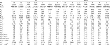
The resolutions obtained for the present cases are reported in table 3. Since a complex equation of state is used for real gases and higher values of the effective Reynolds number are reached, a grid sensitivity study has been conducted and is reported in appendix D. Simulations with PP11 require higher resolution than air to achieve grid convergence of second-order statistics, and the chosen grids in table 3 have quite satisfactory resolution. In our simulations, the overall number of grid points varies between
 $3\times 10^{6}$
and
 $1.2\times 10^{9}$
.
Table 3 summarizes the conditions used for the parametric study. Wall friction Reynolds numbers range from 218.7 to 1017 for air, and from 191.3 to 692.8 for PP11. The semi-local scaling drastically changes the predictions in terms of friction Reynolds number. For air, the friction Reynolds number at the centreline
 $Re_{\unicode[STIX]{x1D70F},c}^{\ast }=Re_{\unicode[STIX]{x1D70F}}^{\ast }(h)$
goes from 88.7 to 324.7, the drop for each case being roughly proportional to
 $M_{B}$
. For PP11, an opposite behaviour is observed:
 $Re_{\unicode[STIX]{x1D70F},c}^{\ast }$
is higher than
 $Re_{\unicode[STIX]{x1D70F}_{w}}$
in each case, and the deviations increase with
 $M_{B}$
. This is due to the different behaviour of the transport properties as it will be explained later. Thus, contrarily to air, the resolution requirements for PP11 are more severe in semi-local scaling than in the classical wall scaling. However, as reported in table 3 and appendix D, the chosen grids ensure a good resolution in each case. Once
 $Re_{\unicode[STIX]{x1D70F}}^{\ast }$
is converged, statistics are collected every ten computational time steps, with
 $\unicode[STIX]{x0394}t^{+}\approx 0.02{-}0.03$
in wall units for all the simulations and during an observation time
 $t_{obs}^{+}$
in the range 1000–3000.
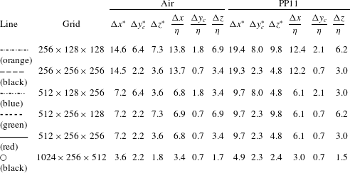
Line styles for the employed DNS cases.

4 Influence of dense-gas effects on flow properties
In this section we first present results for general flow properties and their dependency on the bulk parameters and fluid type. Then, we analyse cross-wise profiles of the first-order statistics. For this purpose, we initially assess different wall scalings, and then focus more specifically on the variations of average thermodynamic properties across the channel, to highlight the peculiar behaviour of dense-gas flows compared with air flows. For the sake of clarity, we investigate the role of compressibility effects by focusing on cases characterized by
 $Re_{B}=7000$
and various Mach numbers. The Reynolds number influence is also studied by considering sets of simulations M1R3 and M3R12. We complete the analysis by discussing dense-gas effects on second-order statistics of the thermodynamic and transport properties. Second-order moments of the velocity fields and, more generally, effects on turbulence structure are discussed in § 5. For these sets of results, each case is uniquely identified with the line style defined in table 2, unless otherwise stated.
Numerical parameters and DNS results for air and PP11.
 $N_{x}$
,
 $N_{y}$
and
 $N_{z}$
are the number of grid points in the streamwise, wall-normal and spanwise directions;
 $Re_{\unicode[STIX]{x1D70F}_{w}}=\overline{\unicode[STIX]{x1D70C}}_{w}u_{\unicode[STIX]{x1D70F}}h/\overline{\unicode[STIX]{x1D707}}_{w}$
is the friction Reynolds number;
 $Re_{\unicode[STIX]{x1D70F},c}^{\ast }=\sqrt{\overline{\unicode[STIX]{x1D70C}}_{c}\unicode[STIX]{x1D70F}_{w}}h/\overline{\unicode[STIX]{x1D707}}_{c}$
is the semi-local friction Reynolds number at the centreline;
 $\unicode[STIX]{x0394}x^{+}$
,
 $\unicode[STIX]{x0394}z^{+}$
,
 $\unicode[STIX]{x0394}y_{w}^{+}$
and
 $\unicode[STIX]{x0394}y_{c}^{+}$
are the mesh sizes in wall units;
 $\unicode[STIX]{x0394}x_{c}^{\ast }$
,
 $\unicode[STIX]{x0394}z_{c}^{\ast }$
and
 $\unicode[STIX]{x0394}y_{c}^{\ast }$
are the mesh sizes in semi-local units;
 $(\unicode[STIX]{x0394}x/\unicode[STIX]{x1D702})_{max}$
,
 $(\unicode[STIX]{x0394}z/\unicode[STIX]{x1D702})_{max}$
,
 $(\unicode[STIX]{x0394}y_{min}/\unicode[STIX]{x1D702})_{max}$
and
 $(\unicode[STIX]{x0394}y_{max}/\unicode[STIX]{x1D702})_{max}$
are the spatial resolutions normalized by the Kolmogorov scale,
 $t_{OBS}^{+}$
is the observation period in wall units;
 $\unicode[STIX]{x0394}t^{+}$
is the computational time step in wall units.

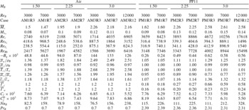
DNS results for air and PP11 cases.
 $\overline{M}_{c}=\overline{u_{c}/c_{c}}$
is the centreline Mach number;
 $M_{\unicode[STIX]{x1D70F}_{w}}=u_{\unicode[STIX]{x1D70F}}/\overline{c}_{w}$
the friction Mach number;
 $Re_{c}=\overline{\unicode[STIX]{x1D70C}}_{c}\overline{u}_{c}h/\overline{\unicode[STIX]{x1D707}}_{c}$
the centreline Reynolds number;
 $Re_{\unicode[STIX]{x1D703}_{w}}=\overline{\unicode[STIX]{x1D70C}}_{w}\overline{u}_{c}\unicode[STIX]{x1D703}/\overline{\unicode[STIX]{x1D707}}_{w}$
the Reynolds number based on momentum thickness
 $\unicode[STIX]{x1D703}$
at wall conditions;
 $Re_{\unicode[STIX]{x1D703}_{c}}=\overline{\unicode[STIX]{x1D70C}}_{c}\overline{u}_{c}\unicode[STIX]{x1D703}/\overline{\unicode[STIX]{x1D707}}_{c}$
the Reynolds number based on momentum thickness at centreline conditions;
 $Re_{Bb}=\unicode[STIX]{x1D70C}_{B}\widetilde{u}_{B}h/\unicode[STIX]{x1D707}_{B}$
the Reynolds number based at bulk conditions;
 $B_{q}=\overline{q}_{w}/(\overline{\unicode[STIX]{x1D70C}}_{w}u_{\unicode[STIX]{x1D70F}}\overline{h}_{w})$
the heat flux at the walls;
 $\overline{\unicode[STIX]{x1D70C}}_{w}/\unicode[STIX]{x1D70C}_{B}$
and
 $\overline{\unicode[STIX]{x1D70C}}_{c}/\unicode[STIX]{x1D70C}_{B}$
the wall and centreline normalized density values;
 $\overline{T}_{c}/\overline{T}_{w}$
,
 $\overline{\unicode[STIX]{x1D707}}_{c}/\overline{\unicode[STIX]{x1D707}}_{w}$
and
 $\overline{c}_{c}/\overline{c}_{w}$
the centreline temperature, viscosity and speed of sound;
 $\overline{\unicode[STIX]{x1D6E4}}_{c}$
and
 $\overline{\unicode[STIX]{x1D6E4}}_{w}$
the centreline and wall values of the fundamental derivative of gas dynamics;
 $C_{f}=2\unicode[STIX]{x1D70F}_{w}/(\unicode[STIX]{x1D70C}_{B}u_{B}^{2})$
the skin friction coefficient;
 $C_{f}^{D}=0.073Re_{m}^{-1/4}$
the skin friction coefficient based on Dean’s correlation (
 $Re_{m}$
is based on bulk quantities and channel height, i.e.
 $Re_{m}=2Re_{Bb}$
);
 $\,Nu_{B}=\overline{q}_{w}D_{h}/(\overline{\unicode[STIX]{x1D705}}_{w}(T_{B}-T_{w}))$
the bulk Nusselt number; and
 $Pr_{B}=\unicode[STIX]{x1D707}_{B}c_{p,B}/\unicode[STIX]{x1D705}_{B}$
the bulk Prandtl number.

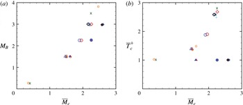
Evolution of
 $M_{B}$
(a) and
 $\overline{T}_{c}^{+}$
(b) as a function of
 $\overline{M}_{c}$
for different cases. Open symbols: air; filled symbols: PP11. Symbol shapes: ▲:
 $M_{B}=1.5$
, ●:
 $M_{B}=2.25$
, ♦:
 $M_{B}=3$
. Symbol colours (online version): red,
 $Re_{B}=3000$
; blue,
 $Re_{B}=7000$
; black,
 $Re_{B}=12\,000$
.
 $+$
(cyan) Coleman et al. (Reference Coleman, Kim and Moser1995),
 $\times$
(green) Foysi et al. (Reference Foysi, Sarkar and Friedrich2004), ○ (orange) Gerolymos & Vallet (Reference Gerolymos and Vallet2014).

4.1 Global flow properties
Table 4 summarizes the main characteristic values of the simulations. Figure 1 provides a first insight into the behaviour of PP11 cases compared to air cases. In this figure,
 $M_{B}$
and
 ${\overline{T}_{c}}^{+}=\overline{T}_{c}/T_{w}$
are plotted as functions of the average centreline Mach number
 $\overline{M}_{c}$
. Values obtained for air cases are in good agreement with reference DNS (Coleman et al.
Reference Coleman, Kim and Moser1995; Foysi et al.
Reference Foysi, Sarkar and Friedrich2004; Gerolymos & Vallet Reference Gerolymos and Vallet2014). For
 $M_{B}\geqslant 1.5$
,
 $\overline{M}_{c}$
is systematically lower than
 $M_{B}$
, since the walls are cooler than the channel core. Indeed for perfect gases,
 $\overline{M}_{c}$
increases nonlinearly since
 $\overline{T}_{c}$
grows rapidly and
 $\overline{c}\propto \sqrt{\overline{T}}$
. The average centreline temperature in figure 1(b) is approximately 1.4 times higher than the wall temperature for AM1R3 and more than 2.5 times higher for AM3R3 due to the significant increase of the viscous heating
 $\overline{\unicode[STIX]{x1D70F}_{ij}\unicode[STIX]{x1D61A}_{ij}}$
. The dependence on the Reynolds number is weak on the considered range, with slightly lower values of
 ${\overline{T}_{c}}^{+}$
for higher
 $Re_{B}$
, which is more clearly appreciated for the highest Mach number conditions. PP11 flows exhibit a rather different behaviour since the molecular complexity of dense gases implies high values of the specific heat
 $c_{v}/R$
and, therefore, the coupling between the thermal and dynamic fields becomes smaller and smaller. Inspection of figure 1(b) indeed shows that the centreline temperature is almost equal to the wall value for any choice of the Mach and Reynolds numbers. Nevertheless, the evolution of
 $\overline{M}_{c}$
changes significantly because in dense gases the speed of sound depends also on density, which decreases moving from the wall to the centreline. In turn,
 $\overline{c}_{c}$
increases leading to lower values of
 $\overline{M}_{c}$
.
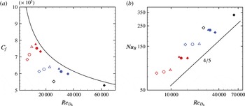
For practical applications, it is interesting to investigate the modifications of momentum and heat transfer coefficients when working with a dense gas. For that purpose, we consider the evolutions of the skin friction coefficient
 $C_{f}$
and the bulk Nusselt number
 $Nu_{B}$
, respectively defined as
 $$\begin{eqnarray}C_{f}=\frac{\unicode[STIX]{x1D70F}_{w}}{\displaystyle {\textstyle \frac{1}{2}}\unicode[STIX]{x1D70C}_{B}u_{B}^{2}};\quad Nu_{B}=\frac{\overline{q}_{w}D_{h}}{\overline{\unicode[STIX]{x1D705}}_{w}(T_{B}-T_{w})},\end{eqnarray}$$
which are depicted in figure 2.
 $D_{h}$
denotes the hydraulic diameter,
 $D_{h}=4h$
for a flat channel. The values predicted by the correlation of Dean (Reference Dean1978), i.e.
 $C_{f}^{D}=0.073Re_{m}^{-1/4}$
, are superimposed in figure 2(a). The correlation has been established in the incompressible regime for
 $Re_{m}>6000$
, where
 $Re_{m}$
is the Reynolds number based on bulk quantities and channel height, i.e.
 $Re_{m}=2Re_{Bb}=\unicode[STIX]{x1D70C}_{B}\widetilde{u}_{B}2h/\unicode[STIX]{x1D707}_{B}$
. For the dense-gas cases, the computed skin friction coefficients are slightly lower than the values predicted by Dean’s correlation, but follow closely the trend with respect to the bulk Reynolds number. The deviations are greater for air ideal flows with an underestimation more pronounced for higher Mach numbers. Some authors (Moneghan Reference Moneghan1953; Huang, Bradshaw & Coakley Reference Huang, Bradshaw and Coakley1993) have proposed compressibility corrections, which work well for turbulent boundary layers over adiabatic walls. A similar extension for channel flows is not without ambiguities since the definition of the freestream values and of the dynamic pressure for normalization are more arbitrary. It can however be concluded that in dense-gas flow decoupling of dynamic and thermal effects dominates, so that Mach number effects are less influential on the skin friction coefficient than in air flows, and Dean’s formula yields a reasonable correlation.
Evolutions of
 $C_{f}$
(a) and
 $Nu_{B}$
(b) as a function of
 $Re_{D_{h}}$
for different cases. Same legend as figure 1.

In a similar manner, the Nusselt number is compared in figure 2(b) with a classical empirical correlation, commonly used to estimate heat transfer in hydraulic pipes (Incropera & DeWitt Reference Incropera and DeWitt2007; Zonta Reference Zonta2013). Specifically, we use the Sieder–Tate correlation,
 $Nu_{B}^{ST}=0.027Re_{D_{h}}^{4/5}Pr_{B}^{1/3}(\unicode[STIX]{x1D707}_{B}/\unicode[STIX]{x1D707}_{w})^{0.14}$
(Sieder & Tate Reference Sieder and Tate1936). Here, the Reynolds number at bulk conditions is based on the hydraulic diameter
 $D_{h}$
, i.e.
 $Re_{D_{h}}=2Re_{m}=4Re_{Bb}$
. This formula is an extension of the Dittus–Boelter/Colburn correlations including the viscosity dependence due to temperature change between the bulk average temperature and wall temperature. Figure 2(b) shows that the power-law exponent of 0.8 captures well the Reynolds number dependence for both fluids. The higher values obtained for dense-gas cases are explained by the Prandtl number dependence, which is constant equal to 0.7 for air and varies between 2.3 and 2.4 for PP11. The enhanced heat capacities of dense gases reduce the heat conduction. A Mach number effect can also be noticed, leading to lower Nusselt numbers when the Mach number increases. This compressibility effect, more visible for air flows, is not taken into account by the empirical correlation. The predicted values of
 $C_{f}$
and
 $Nu_{B}$
are reported in table 4. The heat flux towards the walls
 $B_{q}=\overline{q}_{w}/(\overline{\unicode[STIX]{x1D70C}}_{w}u_{\unicode[STIX]{x1D70F}}\overline{h}_{w})$
, with
 $\overline{h}_{w}$
the specific enthalpy at the wall, is also given. Its order of magnitude is
 $O(10^{0}{-}10^{1})$
for air and
 $O(10^{-4})$
for PP11 flows. Hence, for dense gases, isothermal walls translate also into quasi-adiabatic conditions. Also given in table 4, the wall and centreline mean values of the fundamental derivative
 $\overline{\unicode[STIX]{x1D6E4}}_{w}$
and
 $\overline{\unicode[STIX]{x1D6E4}}_{c}$
are globally lower than unity. Their increase with
 $M_{B}$
is mainly associated with a higher dispersion of the instantaneous thermodynamic states.
4.2 Scalings and first-order statistics
Scalings for the law of the wall for air (top) and PP11 (bottom). (a,d) Classical incompressible scaling
 $\overline{u}^{+}$
; (b,e) Van Driest transformation
 $\overline{u}_{VD}$
; (c,f) Trettel–Larsson transformation
 $\overline{u}_{TL}$
in semi-local coordinates. For the meaning of the line styles in this and subsequent figures, see table 2.

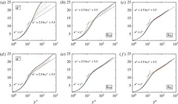
Figure 3 displays the mean streamwise velocity profiles for air (a–c) and PP11 flows (d–f). It is known that the classical incompressible scaling (a,d) fails in collapsing the velocity profiles when compressibility effects are present. In particular, predictions get worse in presence of a substantial heat flux towards the walls. Several attempts have been made in the past in order to derive a transformation able to collapse the compressible velocity profiles into an universal law of the wall for a wide range of Mach numbers. For non-hypersonic flows, Van Driest (Reference Van Driest1951) developed the transformation:
 $$\begin{eqnarray}\overline{u}_{VD}=\int _{0}^{u^{+}}\sqrt{\frac{\overline{\unicode[STIX]{x1D70C}}}{\overline{\unicode[STIX]{x1D70C}}_{w}}}\,\text{d}u^{+},\end{eqnarray}$$
which takes into account mean-density variations and translates the compressible profile into an equivalent ‘constant-density’ profile keeping the same wall-normal coordinate
 $y^{+}$
. The Van Driest transformation provides a substantial improvement of the scaling (b,e), even if it departs from the log law as
 $M_{B}$
increases. The size of the buffer layer increases rapidly for air since the beginning of the logarithmic zone moves towards higher
 $y^{+}$
values (from
 $y^{+}\approx 20$
for AM1R7 to
 $y^{+}\approx 70$
for AM3R12). On the other hand, for dense gases, the heat flux is greatly reduced and
 $\overline{u}_{VD}$
-scaling provides quite satisfactory results. Indeed, this scaling was found to behave well for adiabatic walls (Guarini et al.
Reference Guarini, Moser, Shariff and Wray2000; Pirozzoli, Grasso & Gatski Reference Pirozzoli, Grasso and Gatski2004; Pirozzoli & Bernardini Reference Pirozzoli and Bernardini2011). Modifications for the value of the intercept of the log-law velocity profile,
 $u^{+}=1/\unicode[STIX]{x1D705}_{VK}\log y^{+}+C$
were proposed by Bradshaw (Reference Bradshaw1977), yielding empirical laws that relate
 $C$
to the friction Mach number
 $M_{\unicode[STIX]{x1D70F}}$
and to the heat flux
 $B_{q}$
. Modesti & Pirozzoli (Reference Modesti and Pirozzoli2016) have recently provided a thorough review of the main scalings available in the literature, and have shown that the transformation proposed by Trettel & Larsson (Reference Trettel and Larsson2016),
 $$\begin{eqnarray}\overline{u}_{TL}=\int _{0}^{u^{+}}\sqrt{\frac{\overline{\unicode[STIX]{x1D70C}}}{\overline{\unicode[STIX]{x1D70C}}_{w}}}\left[1+\frac{1}{2}\frac{1}{\overline{\unicode[STIX]{x1D70C}}}\frac{\text{d}\overline{\unicode[STIX]{x1D70C}}}{\text{d}y}y-\frac{1}{\overline{\unicode[STIX]{x1D707}}}\frac{\text{d}\overline{\unicode[STIX]{x1D707}}}{\text{d}y}y\right]\,\text{d}u^{+}\end{eqnarray}$$
accurately reproduces the mean velocity profile even for cases with high wall heat flux. Panels (c,f) confirm its validity even for dense gases. Note that, with this transformation, the wall-normal distance is normalized according to the semi-local scaling
 $y^{\ast }$
.
Profiles of density
 $\overline{\unicode[STIX]{x1D70C}}^{+}$
, temperature
 $\widetilde{T}^{+}$
and pressure
 $\overline{p}/\overline{p}_{w}$
for air (top) and PP11 (bottom) cases. Same legend as in table 2.

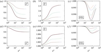
Figure 4 shows the density, temperature and pressure profiles normalized with wall quantities. The semi-local scaling
 $y^{\ast }$
is retained from hereafter as the standard scaling for comparing perfect- and dense-gas cases. The rise of wall density values for increasing
 $M_{B}$
is significant for air and less pronounced for PP11 flows. For instance,
 $\overline{\unicode[STIX]{x1D70C}}/\unicode[STIX]{x1D70C}_{B}=2.51$
for AM3R12 and 1.25 for PM3R12 (see values in table 4). Mean density
 $\overline{\unicode[STIX]{x1D70C}}^{+}$
decreases towards the centreline, with minimum values
 $\min _{y}\{{\overline{\unicode[STIX]{x1D70C}}_{c}}^{+}\}\approx 0.39$
for AM3R3 and
 ${\approx}0.77$
for PM3R3. An eventual influence of the Reynolds number is hidden by the strong dependence on
 $\overline{M}_{c}$
, noticeable for both
 $\overline{\unicode[STIX]{x1D70C}}^{+}$
and
 $\widetilde{T}^{+}$
. As prefigured by figure 1(b), temperature profiles are quite different, with increases lower than 1 % of the wall temperature for PP11 flows. Pressure is roughly constant across the channel. More precisely, it exhibits a constant value in the viscous sublayer, then it slightly decreases in the buffer layer reaching a minimum in the logarithmic zone, and afterwards increases in the outer region. For air, the relationship
 $\overline{p}/\overline{p}_{w}=\overline{\unicode[STIX]{x1D70C}}^{+}\widetilde{T}^{+}\lessapprox 1$
(Gerolymos & Vallet Reference Gerolymos and Vallet2014) holds in each case. The minimum values for air flows are up to three times higher than for PP11 flows, with
 $\max _{y}\{(\overline{p}-\overline{p}_{w})/\overline{p}_{w}\}\approx 1.5\,\%$
for AM3R12 and 0.5 % for PM3R12. Although pressure is nearly constant, its mean value can be directly related to the turbulent fluctuations. In fact, by applying the Favre averaging to the Navier–Stokes equations, one obtains for the mean equation in the
 $y$
-direction (Huang et al.
Reference Huang, Coleman and Bradshaw1995):
 $$\begin{eqnarray}\frac{\unicode[STIX]{x2202}\overline{p}}{\unicode[STIX]{x2202}y}=\frac{\unicode[STIX]{x2202}\overline{\unicode[STIX]{x1D70F}}_{yy}}{\unicode[STIX]{x2202}y}-\frac{\unicode[STIX]{x2202}\overline{\unicode[STIX]{x1D70C}}\widetilde{v^{\prime \prime }v^{\prime \prime }}}{\unicode[STIX]{x2202}y}.\end{eqnarray}$$
For compressible flows, the second term is not equal to zero but remains much lower than the other two. As a consequence, the minimum value of
 $\overline{p}$
coincides with the maximum of the wall-normal Reynolds stresses, as it will be shown later.
Mean profiles of the speed of sound
 $\overline{c}/\overline{c}_{w}$
for air (a) and PP11 (b) flows.

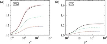
Figure 5 shows the mean profiles of the speed of sound across the channel. Sound speed variations across the channel are related to temperature changes for air (
 $\overline{c}/\overline{c}_{w}=\sqrt{\overline{T}^{+}}$
), whereas they follow density variations for PP11. We notice that relative variations of the speed of sound are much smaller for PP11 (approximately 20 % against 60 % for air), leading to higher values of
 $\overline{M}$
compared to air flows.
Mean profiles of the viscosity
 $\overline{\unicode[STIX]{x1D707}}/\overline{\unicode[STIX]{x1D707}}_{w}$
, the friction Reynolds number
 $Re_{\unicode[STIX]{x1D70F}}^{\ast }$
and the Reynolds number
 $\overline{Re}$
for air (a–c) and PP11 (d–f) flows.

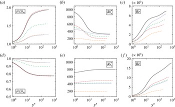
The most striking differences between perfect- and dense-gas flow cases are highlighted in figure 6, presenting the profiles of viscosity, semi-local friction Reynolds number
 $Re_{\unicode[STIX]{x1D70F}}^{\ast }$
and average Reynolds number
 $\overline{Re}$
. For air flows,
 $\overline{\unicode[STIX]{x1D707}}/\overline{\unicode[STIX]{x1D707}}_{w}$
increases towards the centreline (gas-like behaviour), with a maximum deviation in AM3R3 for which
 $\max _{y}\{\overline{\unicode[STIX]{x1D707}}/\overline{\unicode[STIX]{x1D707}}_{w}\}\approx 2$
. For PP11 flows, the ratio decreases (following approximately the
 $\overline{\unicode[STIX]{x1D70C}}^{+}$
profile) up to
 $\min _{y}\{\overline{\unicode[STIX]{x1D707}}/\overline{\unicode[STIX]{x1D707}}_{w}\}\approx 0.75$
for PM3R3, which is a liquid-like behaviour. Viscosity largely influences the profiles of
 $\overline{Re}$
and in particular the centreline values, that tend to be considerably larger for dense gases. The evolution of
 $Re_{\unicode[STIX]{x1D70F}}^{\ast }$
follows opposite behaviours for the two fluids, due to the aforementioned evolutions of transport properties. For air flows, it decreases rapidly up to the logarithmic layer and then more slowly in the outer region. For a given
 $Re_{B}$
, a higher
 $M_{B}$
leads to higher values of
 $Re_{\unicode[STIX]{x1D70F}}^{\ast }$
near the wall, since
 $\overline{\unicode[STIX]{x1D707}}_{w}$
is the same whereas
 $\overline{\unicode[STIX]{x1D70C}}_{w}$
and
 $\overline{(\unicode[STIX]{x2202}u/\unicode[STIX]{x2202}y)}_{w}$
are increasing functions of the Mach number. At greater distance from the wall,
 $Re_{\unicode[STIX]{x1D70F}}^{\ast }$
decreases even more quickly due to the strong temperature gradients in the wall-normal direction. Outside of the viscous sublayer,
 $Re_{\unicode[STIX]{x1D70F}}^{\ast }$
is considerably lower than the near-wall one for the higher
 $M_{B}$
cases, due to the combined effect of a rapid decrease of local density and an increase of local viscosity. Specifically, the centreline value may drop below the one obtained for lower Mach number cases, for which the fluid properties vary less. For PP11 flows,
 $Re_{\unicode[STIX]{x1D70F}}^{\ast }$
exhibits an opposite behaviour, namely, it increases when moving from the wall to the centreline. The overall variations, of the order of 12 % at most for high Mach number cases, are anyway much smaller than in the perfect gas (variations up to 60 %). When increasing the wall distance,
 $Re_{\unicode[STIX]{x1D70F}}^{\ast }$
slightly increases up to the buffer layer and remains roughly constant afterwards. Due to the increasing reduction of centreline viscosity for higher Mach number cases, the growth of
 $Re_{\unicode[STIX]{x1D70F}}^{\ast }$
is enhanced when
 $M_{B}$
becomes higher. The liquid-like viscosity behaviour clearly affects the profile of the local Reynolds number
 $\overline{Re}$
(panel f) compared to the perfect gas (panel c). For instance, at the centreline,
 $\overline{Re}_{c}$
is about 2.5 times higher for PM3R12 than for AM3R12 results.
Mean profiles of the Prandtl number
 $\overline{Pr}$
(a), specific heat at constant pressure
 $\overline{c_{p}}/R$
(b) for PP11 and Eckert number
 $\overline{Ec}$
(c) for air and PP11.

A direct consequence of the constant Prandtl number assumption in the ideal model is that
 $\overline{\unicode[STIX]{x1D705}}/\overline{\unicode[STIX]{x1D705}}_{w}=\overline{\unicode[STIX]{x1D707}}/\overline{\unicode[STIX]{x1D707}}_{w}$
for air. In PP11 simulations, variations of the thermal conductivity across the channel are smaller than the ones of viscosity (
 $\min _{y}\{\overline{\unicode[STIX]{x1D705}}/\overline{\unicode[STIX]{x1D705}}_{w}\}\approx 0.95$
), nevertheless the ratio of the two transport properties remains roughly constant and
 $\overline{\unicode[STIX]{x1D707}}/\overline{\unicode[STIX]{x1D705}}\approx 1.25$
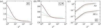
throughout the channel. Thus, the Prandtl number profile (figure 7
a) is essentially driven by the normalized specific heat at constant pressure
 $\overline{c_{p}}/R$
(figure 7
b) which, in turn, follows a trend similar to the density profile (i.e. decreases with the wall distance). As pointed out in the above, the latter exhibit a strong dependency on
 $M_{B}$
in the near-wall region, which is then fed back to
 $\overline{Pr}$
. Specifically, the wall Prandtl number increases by approximately 50 % when doubling the bulk Mach number and is almost insensitive to the Reynolds number. In the outer region,
 $\overline{Pr}\approx 2.3-2.4$
for all dense-gas cases. On the other hand, the high values of
 $\overline{c_{p}}/R$
for dense gases lead to very small values of the average Eckert number,
 $\overline{Ec}=\overline{u^{2}/c_{p}T}$
, a parameter that is representative of the degree of coupling between thermal and kinematic effects. We recall that for air flows,
 $\overline{c_{p}}/R=c_{p}/R=3.5$
, which is two orders of magnitude lower than the mean values obtained with PP11. In figure 7(c),
 $\overline{Ec}$
exhibits a similar trend for both fluids, with two logarithmic zones connected near
 $y^{\ast }\approx 15$
, but the curves are shifted by approximately two orders of magnitude. In fact, the centreline values are of the order of
 $O(1)$
for air and
 $O(10^{-2})$
for PP11 cases.
4.3 Second-order statistics of the thermodynamic and transport properties
Profiles of the normalized root mean square density
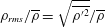 $\unicode[STIX]{x1D70C}_{rms}/\overline{\unicode[STIX]{x1D70C}}=\sqrt{\overline{\unicode[STIX]{x1D70C}^{\prime 2}}}/\overline{\unicode[STIX]{x1D70C}}$
(a,d), temperature
 $T_{rms}/\overline{T}=\sqrt{\overline{T^{\prime 2}}}/\overline{T}$
(b,e) and pressure
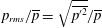 $p_{rms}/\overline{p}=\sqrt{\overline{p^{\prime 2}}}/\overline{p}$
(c,f) for air flows (a–c) and PP11 flows (d–f).

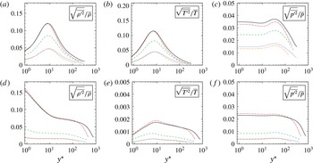
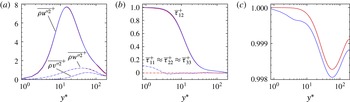
Root mean square (r.m.s.) values for the density, temperature and pressure are shown in figure 8. Gerolymos & Vallet (Reference Gerolymos and Vallet2014) have shown that for air flows
 $O(T_{rms}/\overline{T})=O(\unicode[STIX]{x1D70C}_{rms}/\overline{\unicode[STIX]{x1D70C}})=O(p_{rms}/\overline{p})$
, regardless of the
 $y^{\ast }$
location, Mach and Reynolds numbers. The same trend has been observed for both forced (Donzis & Jagannathan Reference Donzis and Jagannathan2013) and decaying (Sciacovelli et al.
Reference Sciacovelli, Cinnella, Content and Grasso2016a
) highly compressible homogeneous turbulence. As discussed in Gerolymos & Vallet (Reference Gerolymos and Vallet2014), this behaviour is a direct consequence of the perfect-gas equation of state, and does not depend on the specific flow configuration under investigation. Indeed, writing the differential form of the ideal-gas law
 $(\text{d}p/p)=(\text{d}\unicode[STIX]{x1D70C}/\unicode[STIX]{x1D70C})+(\text{d}T/T)$
and approximating differential terms by r.m.s. fluctuations, we get:
 $$\begin{eqnarray}\frac{p_{rms}}{\overline{p}}\approx \frac{\unicode[STIX]{x1D70C}_{rms}}{\overline{\unicode[STIX]{x1D70C}}}+\frac{T_{rms}}{\overline{T}}.\end{eqnarray}$$
After an initial growth in the linear region,
 $\unicode[STIX]{x1D70C}_{rms}/\overline{\unicode[STIX]{x1D70C}}$
and
 $T_{rms}/\overline{T}$
reach a peak in the buffer layer at
 $y^{\ast }\approx 10$
and then decay. The pressure fluctuations are rather nearly constant close to the walls, slightly peak at the beginning of the logarithmic zone (
 $y^{\ast }\approx 40$
) and finally decrease, reaching a minimum in the core region. Since pressure fluctuations are of smaller order whereas
 $\unicode[STIX]{x1D70C}_{rms}/\overline{\unicode[STIX]{x1D70C}}$
and
 $T_{rms}/\overline{T}$
have very similar distributions and levels, equation (4.5) permits one to identify temperature with density fluctuations, corresponding to the assumption of Laufer (Reference Laufer1969) of essentially isobaric temperature fluctuations. Some authors (Rubesin Reference Rubesin1990; Huang et al.
Reference Huang, Coleman and Bradshaw1995) propose rather that the gas behaves generally in a polytropic manner.
For dense gases, the observed trends are very different. While the overall levels of density and pressure fluctuations remain of the same order of magnitude as for air cases, the relative temperature fluctuations are more than one order of magnitude lower. The fluctuating pressure distribution is much like the perfect-gas one, since it depends on the fluctuating velocity through a Poisson equation. Furthermore, the r.m.s. density decreases monotonically with the wall distance, the highest density fluctuations being observed close to the walls. The r.m.s. density levels decay at higher rates in the linear layer and in the outer region, and exhibit only weak variations in the logarithmic region. This behaviour can also be directly related to the equation of state, namely the Martin–Hou equation (2.10). Following the same reasoning as for the ideal gas, the differential form
 $dp=(\unicode[STIX]{x2202}p/\unicode[STIX]{x2202}\unicode[STIX]{x1D70C})_{T}d\unicode[STIX]{x1D70C}+(\unicode[STIX]{x2202}p/\unicode[STIX]{x2202}T)_{\unicode[STIX]{x1D70C}}\,\text{d}T$
is derived and the differential terms are approximated by r.m.s. fluctuations, yielding:
 $$\begin{eqnarray}\frac{\unicode[STIX]{x1D70C}_{rms}}{\overline{\unicode[STIX]{x1D70C}}}\approx \frac{1}{\overline{\unicode[STIX]{x1D70C}}}\left.\left[p_{rms}-\left(\frac{\unicode[STIX]{x2202}p}{\unicode[STIX]{x2202}T}\right)_{\unicode[STIX]{x1D70C}}T_{rms}\right]\right/\left(\frac{\unicode[STIX]{x2202}p}{\unicode[STIX]{x2202}\unicode[STIX]{x1D70C}}\right)_{T},\end{eqnarray}$$
where the partial derivatives are evaluated from mean quantities:
 $$\begin{eqnarray}\displaystyle & \displaystyle \left(\frac{\unicode[STIX]{x2202}p}{\unicode[STIX]{x2202}\unicode[STIX]{x1D70C}}\right)_{T}\approx \frac{R\overline{T}}{(1-\overline{\unicode[STIX]{x1D70C}}b)^{2}}+\mathop{\sum }_{i=2}^{5}\frac{i\overline{\unicode[STIX]{x1D70C}}^{i-1}f_{i}(\overline{T})}{(1-\overline{\unicode[STIX]{x1D70C}}b)^{i+1}} & \displaystyle\end{eqnarray}$$
 $$\begin{eqnarray}\displaystyle & \displaystyle \left(\frac{\unicode[STIX]{x2202}p}{\unicode[STIX]{x2202}T}\right)_{\unicode[STIX]{x1D70C}}\approx \frac{\overline{\unicode[STIX]{x1D70C}}R}{1-\overline{\unicode[STIX]{x1D70C}}b}+\mathop{\sum }_{i=2}^{5}\frac{\overline{\unicode[STIX]{x1D70C}}^{i}f_{i}^{\prime }(\overline{p})}{(1-\overline{\unicode[STIX]{x1D70C}}b)^{i}}\quad \text{with}~f_{i}^{\prime }(\overline{T})=B_{i}-(kC_{i}/T_{cr})\exp (-k\overline{T}/T_{cr}). & \displaystyle \nonumber\\ \displaystyle & & \displaystyle\end{eqnarray}$$
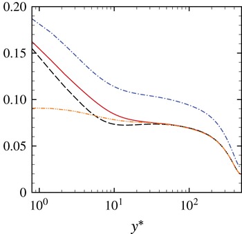
The validity of the approximated relation (4.6) is checked in figure 9 for case PM3R7 against DNS results for
 $\unicode[STIX]{x1D70C}_{rms}/\overline{\unicode[STIX]{x1D70C}}$
and appears to be reasonably accurate, especially concerning the observed trends. Then, considering that the thermal variations are weak for the dense-gas temperature fluctuations are neglected, i.e.
 $T_{rms}=0$
in (4.6). The corresponding curve follows fairly the trends of
 $\unicode[STIX]{x1D70C}_{rms}/\overline{\unicode[STIX]{x1D70C}}$
. The isothermal assumption is then a good approximation for the dense gas, meaning (i) that density fluctuations are correlated with pressure fluctuations and (ii) that
 $\unicode[STIX]{x1D70C}_{rms}/\overline{\unicode[STIX]{x1D70C}}$
is well approximated by
 $(p_{rms}/\overline{\unicode[STIX]{x1D70C}})/(\unicode[STIX]{x2202}p/\unicode[STIX]{x2202}\unicode[STIX]{x1D70C})_{T}$
.
Finally, using the definition of the sound speed
 $c^{2}=(\unicode[STIX]{x2202}p/\unicode[STIX]{x2202}\unicode[STIX]{x1D70C})_{s}$
, and replacing the partial derivative of
 $p$
with respect to
 $\unicode[STIX]{x1D70C}$
at constant
 $T$
by the same partial derivative at constant entropy yields
 $(p_{rms}/\overline{\unicode[STIX]{x1D70C}})/\overline{c}^{2}$
. The proportionality with the fluid compressibility (inverse of the speed of sound squared) is also tested in figure 9. A good match is obtained above the viscous sublayer, which means that the assumption that the isothermal approximation is also close to an adiabatic approximation for a dense gas is globally true, except very near to the wall. The preceding discussion shows that the rise of density fluctuations near the wall is related to the peculiar behaviour of the thermal equation of state for a nearly isothermal process. Similar results (not shown) were also obtained for a simpler thermal equation of state (Van der Waals) with the same qualitative behaviour, under the polytropic-gas assumption.
Despite the complex variations, fluctuations in thermophysical quantities globally remains moderate for PP11. As a consequence, the assumption of Morkovin (Reference Morkovin and Favre1961), stating that the entropy and vortical modes are weakly coupled, is still valid. Fluctuation levels up to 18 % of the mean value are noticed very near the wall for the density, but this region is dominated by viscous stresses, so that the conclusion is not altered.
Approximation of normalized density fluctuations for case PM3R7. —— (red)
 $\unicode[STIX]{x1D70C}_{rms}/\overline{\unicode[STIX]{x1D70C}}$
;
- - - - - (black)
 $[p_{rms}-(\unicode[STIX]{x2202}p/\unicode[STIX]{x2202}T)_{\unicode[STIX]{x1D70C}}T_{rms}]/(\unicode[STIX]{x2202}p/\unicode[STIX]{x2202}\unicode[STIX]{x1D70C})_{T}/\overline{\unicode[STIX]{x1D70C}}$
;
 $\boldsymbol{-}\cdot \boldsymbol{-}\cdot \boldsymbol{-}\cdot \boldsymbol{-}\cdot \boldsymbol{-}\cdot$
(blue)
 $p_{rms}/(\unicode[STIX]{x2202}p/\unicode[STIX]{x2202}\unicode[STIX]{x1D70C})_{T}/\overline{\unicode[STIX]{x1D70C}}$
;
 $\boldsymbol{-}\cdot \cdot \boldsymbol{-}\cdot \cdot \boldsymbol{-}\cdot \cdot$
(orange)
 $p_{rms}/\overline{c}^{2}/\overline{\unicode[STIX]{x1D70C}}$
.

Profiles of the correlation coefficients
 $C_{\unicode[STIX]{x1D70C}^{\prime }p^{\prime }}$
(a,e),
 $C_{\unicode[STIX]{x1D70C}^{\prime }u^{\prime }}$
(b,f),
 $C_{\unicode[STIX]{x1D70C}^{\prime }v^{\prime }}$
(c,g) and
 $C_{u^{\prime }v^{\prime }}$
(d,h) for air (a–d) and PP11 MAH (e–h) flows.

To further clarify the strong relations between density and pressure, correlation coefficients are calculated. Given two flow variables
 $\unicode[STIX]{x1D6FC}$
and
 $\unicode[STIX]{x1D6FD}$
, the correlation coefficient
 $C_{\unicode[STIX]{x1D6FC}^{\prime }\unicode[STIX]{x1D6FD}^{\prime }}$
is defined as:
 $$\begin{eqnarray}C_{\unicode[STIX]{x1D6FC}^{\prime }\unicode[STIX]{x1D6FD}^{\prime }}=\frac{\overline{\unicode[STIX]{x1D6FC}^{\prime }\unicode[STIX]{x1D6FD}^{\prime }}}{\sqrt{\overline{\unicode[STIX]{x1D6FC}^{\prime 2}}}\sqrt{\overline{\unicode[STIX]{x1D6FD}^{\prime 2}}}}.\end{eqnarray}$$
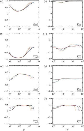
Figure 10 shows the correlations
 $C_{\unicode[STIX]{x1D70C}^{\prime }p^{\prime }}$
,
 $C_{\unicode[STIX]{x1D70C}^{\prime }u^{\prime }}$
,
 $C_{\unicode[STIX]{x1D70C}^{\prime }v^{\prime }}$
and
 $C_{u^{\prime }v^{\prime }}$
. Due to the isothermal boundary conditions, the correlation coefficient
 $C_{\unicode[STIX]{x1D70C}^{\prime }p^{\prime }}$
is equal to unity at the walls for both air and PP11. Afterwards, it decreases reaching a minimum at
 $y^{\ast }\approx 8$
, approximately corresponding to the temperature variance peak, and then it increases again towards the centreline. For PP11 flows
 $C_{\unicode[STIX]{x1D70C}^{\prime }p^{\prime }}$
approaches unity already at
 $y^{\ast }\approx 20$
and then remains constant. On the other hand, it raises slowly for air flows, with an asymptotic value close to 0.9. The correlation coefficients
 $C_{\unicode[STIX]{x1D70C}^{\prime }u^{\prime }}$
and
 $C_{\unicode[STIX]{x1D70C}^{\prime }v^{\prime }}$
, which represent the transport of density fluctuations by the streamwise and wall-normal velocities, exhibit a totally different evolution depending on the fluid nature. Specifically, for air the streamwise correlation is negative and the spanwise is positive, whereas for PP11 both coefficients tend rapidly towards zero. Furthermore,
 $C_{\unicode[STIX]{x1D70C}^{\prime }u^{\prime }}$
exhibits both a Mach and Reynolds dependence for air, whereas for PP11 it varies only with the Mach number. Lastly, the distributions
 $C_{u^{\prime }v^{\prime }}$
are similar even if a perfect collapse can be noticed for air, whereas a slight Mach dependence is observed for PP11.
Distribution of
 $p-v$
states of an instantaneous flow field for PP11 in a Clapeyron’s diagram. (a) Influence of Mach number on the distribution of
 $p-v$
states for a slice at
 $y^{\ast }\approx 10$
and
 $Re_{B}=3000$
: (○, red)
 $M_{B}=1.5$
; (●)
 $M_{B}=2.25$
; (○)
 $M_{B}=3$
. The background colour map shows isocontours of the speed of sound. (b) Influence of Reynolds number on the distribution of
 $p-v$
states for a slice at
 $y^{\ast }\approx 10$
and
 $M_{B}=3$
: (○, red)
 $Re_{B}=3000$
; (●)
 $Re_{B}=7000$
; (○)
 $Re_{B}=12\,000$
. The background colour map shows isocontours of the viscosity. (c) Influence of
 $y^{\ast }$
location on the distribution of
 $p-v$
states for
 $M_{B}=3$
and
 $Re_{B}=12\,000$
: (○, red)
 $y^{\ast }=798$
(centreline); (●)
 $y^{\ast }=50$
; (○)
 $y^{\ast }=10$
. The background colour map shows isocontours of the Prandtl number.

Another way to interpret the peculiar behaviour of the thermodynamic quantities is to look at representations in Clapeyron’s diagrams. Figure 11 shows distributions of the
 $p-v$
states in the computational box at one instant for PP11 flows. The different panels correspond successively to the influence of
 $M_{B}$
,
 $Re_{B}$
and the wall-normal position. The different
 $p-v$
diagrams are coloured successively with values of the speed of sound, viscosity and Prandtl number in order to highlight the differences with respect to air. The
 $p-v$
states are recorded on slices parallel to the wall. The location is fixed at
 $y^{\ast }\approx 10$
where temperature fluctuations peak for figure 11(a,b). It is clear from figure 11(a) that the main effect of increasing
 $M_{B}$
is a broadening of the region spanned by the
 $p-v$
states. For
 $M_{B}=3$
cases, the states characterized by stronger compressions exit the dense-gas region and reach a supercritical zone where strong variations of the thermodynamic properties are observed. Higher values of
 $M_{B}$
imply a greater dispersion in
 $\overline{\unicode[STIX]{x1D70C}}_{w}$
values and in variances of the thermodynamic variables near the wall. Changing the Reynolds number
 $Re_{B}$
for a given
 $M_{B}$
in figure 11(b) reveals that the distributions of
 $p-v$
states are almost superimposed for the same
 $y^{\ast }$
, providing an a posteriori check of the validity of the semi-local scaling. Lastly, distributions for different
 $y^{\ast }$
values are shown in figure 11(c). The thermodynamic regions spanned by the
 $p-v$
states are reduced moving away from the wall. Even if most of the states are enclosed in the dense-gas region, none of the present simulations exhibit peculiar dense-gas effects, such as expansion shock waves. This can be explained by the fact that the turbulent Mach number,
 $M_{t}=\sqrt{u_{i}^{\prime 2}}/\overline{c}$
, does not reach sufficiently high values. For instance, figure 12 indicates that
 $M_{t}$
approaches 0.4 for
 $M_{B}=3$
, whereas Sciacovelli et al. (Reference Sciacovelli, Cinnella, Content and Grasso2016a
) have shown that significant dense-gas effects can appear for
 $M_{t}$
above 0.8. The distributions of
 $M_{t}$
are similar as the simulations with air with slightly higher values for PP11 flows, showing that, notwithstanding liquid-like characteristics of dense gases, important compressibility is also present. The profiles of the fundamental derivative of gas dynamics
 $\overline{\unicode[STIX]{x1D6E4}}$
, plotted in figure 12(c), confirm that mean values are indeed lower than 1 for PP11 flows, with minimal values in the channel core. The flows thus evolve in the dense-gas region but with positive values of
 $\overline{\unicode[STIX]{x1D6E4}}$
, so that BZT phenomena are not expected.
Profiles of the turbulent Mach number
 $M_{t}$
for air (a) and PP11 (b) and of the fundamental derivative of gas dynamics
 $\overline{\unicode[STIX]{x1D6E4}}$
for PP11 (c).

5 Influence of dense-gas effects on turbulence structure
5.1 Reynolds stresses and Fukagata–Iwamoto–Kasagi (FIK) identity
Reynolds stresses in the streamwise (a,e), wall-normal (b,f) and spanwise (c,g) directions and Reynolds shear stresses (d,h) for air (a–d) and PP11 (e–h) flows with semi-local scaling.

Figure 13 shows the Reynolds stresses
 $[\overline{\unicode[STIX]{x1D70C}u_{i}^{\prime \prime }u_{j}^{\prime \prime }}]^{+}=\overline{\unicode[STIX]{x1D70C}u_{i}^{\prime \prime }u_{j}^{\prime \prime }}/\unicode[STIX]{x1D70F}_{w}$
for the selected simulations. Patel et al. (Reference Patel, Peeters, Boersma and Pecnik2015) have shown that for variable-property turbulent channel flows, gas-like transport properties tend to lower the spanwise, wall-normal and shear Reynolds stresses with respect to the corresponding incompressible evolution, whereas the streamwise component increases. The opposite trend is expected when liquid-like properties are considered. In our cases the strong compressibility adds a complexity in the sense that higher
 $M_{B}$
increase the velocity gradients near the wall (thus increasing the Reynolds stresses) but also dramatically affect viscosity distributions. Figure 13 provides the trends of Reynolds stresses as a function of both Reynolds and Mach number for selected air and PP11 flows. The figure shows that the Reynolds number dependency is the same for the ideal or dense gas, and is similar to that observed for incompressible flows, even if compressibility effects modify the effective friction Reynolds number for a given bulk Reynolds number. For instance, case AM1R7 (
 $Re_{\unicode[STIX]{x1D70F}}^{\ast }\approx 315$
) is characterized by a semi-local friction Reynolds number higher than case AM3R7 (
 $Re_{\unicode[STIX]{x1D70F}}^{\ast }\approx 200$
). On the contrary, the dependency on the bulk Mach number is different for the two fluids. In air, the temperature increases with
 $M_{B}$
, and so does the viscosity, leading to lower values of
 $\overline{\unicode[STIX]{x1D70C}v^{\prime \prime }v^{\prime \prime }}^{+}$
,
 $\overline{\unicode[STIX]{x1D70C}w^{\prime \prime }w^{\prime \prime }}^{+}$
,
 $\overline{\unicode[STIX]{x1D70C}u^{\prime \prime }v^{\prime \prime }}^{+}$
as
 $M_{B}$
grows. For PP11, the viscosity (following the density) becomes lower and lower, thus enhancing the spanwise, cross-wise and shear Reynolds stresses. For the streamwise stress, instead, the same behaviour is observed between air and PP11 since the effect of viscosity is now overwhelmed by the increase of the mean velocity shear across the channel.
Concerning the location of the peak values, for both air and PP11 flows they are roughly constant for the streamwise and spanwise components, namely around
 $y^{\ast }\in [10,13]$
for
 $\overline{\unicode[STIX]{x1D70C}u^{\prime \prime 2}}^{+}$
, and
 $y^{\ast }\in [40,50]$
for
 $\overline{\unicode[STIX]{x1D70C}w^{\prime \prime 2}}^{+}$
. On the other hand, a weak dependence on
 $Re$
is observed for wall-normal and shear stresses. The slight shift towards higher
 $y^{\ast }$
is more pronounced for PP11 flows since much higher
 $Re_{\unicode[STIX]{x1D70F}}^{\ast }$
are achieved. The
 $Re$
influence is consistent with high Reynolds number incompressible simulations (Lee & Moser Reference Lee and Moser2015). It can be noticed that wall-normal stresses
 $\overline{\unicode[STIX]{x1D70C}v^{\prime \prime }v^{\prime \prime }}^{+}$
for PP11 flows present different centreline values, notably for cases PM3R7 and PM3R12 at
 $M_{B}=3$
. The levels of wall-normal fluctuations become then of the same level as those in the streamwise direction.
The contribution of Reynolds stresses to the skin friction coefficient can be analysed thanks to the FIK identity. This decomposition of sources of friction also reveals important differences between ideal and dense gases. Starting from the incompressible expression of Fukagata, Iwamoto & Kasagi (Reference Fukagata, Iwamoto and Kasagi2002), Gomez, Flutet & Sagaut (Reference Gomez, Flutet and Sagaut2009) derived an exact relationship for the analysis of the contribution of Reynolds stresses to the skin friction coefficient in compressible cases. The skin friction coefficient may be split into four contributions, namely:
 $$\begin{eqnarray}\displaystyle C_{f}^{FIK} & = & \displaystyle \underbrace{\frac{6}{Re_{B}}}_{C_{L}}+\underbrace{6\int _{0}^{1}(1-y)\overline{\unicode[STIX]{x1D70C}}(\widetilde{-u^{\prime \prime }v^{\prime \prime }})\,\text{d}y}_{C_{T}}+\underbrace{\frac{6}{Re_{B}}\int _{0}^{1}(1-y)\overline{\widehat{\unicode[STIX]{x1D707}}}\frac{\unicode[STIX]{x2202}\overline{u}}{\unicode[STIX]{x2202}y}\,\text{d}y}_{C_{C}}\nonumber\\ \displaystyle & & \displaystyle +\,\underbrace{\frac{6}{Re_{B}}\int _{0}^{1}(1-y)\overline{\unicode[STIX]{x1D707}^{\prime }\left(\frac{\unicode[STIX]{x2202}u^{\prime }}{\unicode[STIX]{x2202}y}+\frac{\unicode[STIX]{x2202}v^{\prime }}{\unicode[STIX]{x2202}x}\right)}\,\text{d}y}_{C_{CT}},\end{eqnarray}$$
where
 $C_{L}$
is the laminar contribution,
 $C_{T}$
the turbulent contribution,
 $C_{C}$
the compressible contribution (in which
 $\overline{\widehat{\unicode[STIX]{x1D707}}}=\overline{\unicode[STIX]{x1D707}}-1$
) and
 $C_{CT}$
the compressible–turbulent interaction term. Note that all the quantities in (5.1) are non-dimensionalized using the channel half-width
 $h$
as length scale,
 $\widetilde{u}_{B}$
as velocity scale,
 $\unicode[STIX]{x1D70C}_{B}$
as density scale and
 $\overline{\unicode[STIX]{x1D707}}_{w}$
as viscosity scale. As observed by Fukagata et al. (Reference Fukagata, Iwamoto and Kasagi2002), the turbulent term is proportional to the Favre-averaged Reynolds stresses, and the weighting term decreases linearly with the distance from the wall. This explains why the main contribution to the frictional drag is due to the turbulent structures close to the wall, rather than at the location of the peak of Reynolds stresses. The compressible term
 $C_{C}$
is related to the mean viscosity variations and to the mean wall-normal velocity gradient.
 $C_{CT}$
represents the interaction between compressibility and turbulent effects and is usually very small. Table 5 gives the values of
 $C_{f}^{FIK}$
for different cases, as well as the relative error with respect to the values obtained in § 4.1 and the relative percentage of each contribution. To investigate the effect of compressibility, we consider the cases with
 $Re_{B}=7000$
and different
 $M_{B}$
, such that the laminar contribution
 $C_{L}$
is approximately constant (i.e.
 $C_{L}\approx 13\,\%$
–
 $14\,\%$
). For air flows, the contribution due to the turbulent fluctuations
 $C_{T}$
decreases as
 $M_{B}$
increases, coherently with the decreasing of the Reynolds stress levels. The opposite trend is observed for PP11 flows, for which the relative weight of
 $C_{T}$
increases of approximately 1.5 %. This can be related to the liquid-like behaviour of dense gases, which also causes substantial changes in the compressible contribution
 $C_{C}$
. In fact this term takes on higher values as
 $M_{B}$
increases for both fluids, but it is positive for air (since
 $\overline{\widehat{\unicode[STIX]{x1D707}}}>0$
) and negative for PP11 (
 $\overline{\widehat{\unicode[STIX]{x1D707}}}<0$
). The compressible term is indeed related to variable-property effects. Lastly, the compressible–turbulent interaction term is always quite small and contributes to the total skin friction coefficient for approximately 0.1 % in air and 0.02 % in PP11 flows, for which the dynamic and thermal effects are even less correlated.
Contributions to the skin friction coefficient according to the compressible extension of the FIK identity of Gomez et al. (Reference Gomez, Flutet and Sagaut2009) for different cases.
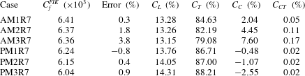
5.2 Turbulent kinetic energy budgets
For fully developed, statistically stationary channel flow, the turbulent kinetic energy budget reads
 $P_{k}+T_{k}+V_{k}+M_{k}+\unicode[STIX]{x1D60B}_{k}+\unicode[STIX]{x1D700}_{k}=0$
, with
 $$\begin{eqnarray}\displaystyle & \displaystyle P_{k}=-\overline{\unicode[STIX]{x1D70C}}\widetilde{u^{\prime \prime }v^{\prime \prime }}\frac{\text{d}\tilde{u} }{\text{d}y} & \displaystyle\end{eqnarray}$$
 $$\begin{eqnarray}\displaystyle & \displaystyle T_{k}=-\frac{\text{d}}{\text{d}y}\frac{1}{2}(\overline{\unicode[STIX]{x1D70C}u^{\prime \prime 2}v^{\prime \prime }}+\overline{\unicode[STIX]{x1D70C}{v^{\prime \prime }}^{3}}+\overline{\unicode[STIX]{x1D70C}w^{\prime \prime 2}v^{\prime \prime }}) & \displaystyle\end{eqnarray}$$
 $$\begin{eqnarray}\displaystyle & \displaystyle V_{k}=\frac{\text{d}}{\text{d}y}(\overline{u^{\prime }\unicode[STIX]{x1D70F}_{xy}^{\prime }}+\overline{v^{\prime }\unicode[STIX]{x1D70F}_{yy}^{\prime }}+\overline{w^{\prime }\unicode[STIX]{x1D70F}_{yz}^{\prime }}) & \displaystyle\end{eqnarray}$$
 $$\begin{eqnarray}\displaystyle & \displaystyle M_{k}=\overline{u^{\prime \prime }}\left(-\frac{\unicode[STIX]{x2202}\overline{p}}{\unicode[STIX]{x2202}x}+\frac{\text{d}\overline{\unicode[STIX]{x1D70F}_{xy}}}{\text{d}y}\right)+\overline{v^{\prime \prime }}\left(-\frac{\unicode[STIX]{x2202}\overline{p}}{\unicode[STIX]{x2202}y}+\frac{\text{d}\overline{\unicode[STIX]{x1D70F}_{yy}}}{\text{d}y}\right)+\overline{w^{\prime \prime }}\frac{\text{d}\overline{\unicode[STIX]{x1D70F}_{yz}}}{\text{d}y} & \displaystyle\end{eqnarray}$$
 $$\begin{eqnarray}\displaystyle & \displaystyle \unicode[STIX]{x1D60B}_{k}=\overline{p^{\prime }\frac{\unicode[STIX]{x2202}u^{\prime }}{\unicode[STIX]{x2202}x}}+\overline{p^{\prime }\frac{\unicode[STIX]{x2202}v^{\prime }}{\unicode[STIX]{x2202}y}}-\frac{\text{d}}{\text{d}y}\overline{v^{\prime }p^{\prime }}+\overline{p^{\prime }\frac{\unicode[STIX]{x2202}w^{\prime }}{\unicode[STIX]{x2202}z}} & \displaystyle\end{eqnarray}$$
 $$\begin{eqnarray}\displaystyle & \displaystyle \unicode[STIX]{x1D700}_{k}=\,-\!\left(\overline{\unicode[STIX]{x1D70F}_{xj}^{\prime }\frac{\unicode[STIX]{x2202}u^{\prime }}{\unicode[STIX]{x2202}x_{j}}}+\overline{\unicode[STIX]{x1D70F}_{yj}^{\prime }\frac{\unicode[STIX]{x2202}v^{\prime }}{\unicode[STIX]{x2202}x_{j}}}+\overline{\unicode[STIX]{x1D70F}_{zj}^{\prime }\frac{\unicode[STIX]{x2202}w^{\prime }}{\unicode[STIX]{x2202}x_{j}}}\right) & \displaystyle\end{eqnarray}$$
 $P_{k}$
is the production,
 $T_{k}$
and
 $V_{k}$
the turbulent and viscous transport respectively,
 $M_{k}$
the mass flux variation,
 $\unicode[STIX]{x1D60B}_{k}$
the velocity–pressure gradient tensor (composed of the sum of pressure strain correlation and pressure transport term) and
 $\unicode[STIX]{x1D700}_{k}$
the dissipation term. Figure 14 shows the turbulent kinetic energy budget for cases AM3R12 and PM3R12 normalized by
 $\unicode[STIX]{x1D70F}_{w}^{2}/\overline{\unicode[STIX]{x1D707}}(y)$
(Foysi et al.
Reference Foysi, Sarkar and Friedrich2004). In semi-local scaling, the viscous and turbulent transports behave similarly, whereas the mass flux variation (which is zero for incompressible flows) is much smaller for PP11 case. In the core region, all the budget terms collapse.
Comparison of turbulent kinetic energy budgets for cases AM3R12 (dashed lines) and PM3R12 (solid lines) in semi-local scaling: —— (red)
 $P_{k}$
, —— (green)
 $T_{k}$
, —— (blue)
 $V_{k}$
, —— (black)
 $M_{k}$
, —— (purple)
 $\unicode[STIX]{x1D60B}_{k}$
, —— (orange)
 $\unicode[STIX]{x1D700}_{k}$
normalized by
 $\unicode[STIX]{x1D70F}_{w}^{2}/\overline{\unicode[STIX]{x1D707}}(y)$
.

Profiles of the turbulent production
 $P_{k}$
, the turbulent dissipation
 $\unicode[STIX]{x1D700}_{k}$
and the ratio of production to dissipation
 $P_{k}/\unicode[STIX]{x1D700}_{k}-1$
for air (a,b) and PP11 (c,d) flows.

A closer inspection of the turbulent production and dissipation for the selected simulations is provided in figure 15, which also shows their ratio, plotted both in linear and logarithmic semi-local coordinates. For both fluids, the production peak is located at
 $y^{\ast }\approx 11$
–12 for all the considered bulk conditions. Sarkar (Reference Sarkar1995) and Lechner et al. (Reference Lechner, Sesterhenn and Friedrich2001) showed that the main effect of compressibility is a reduction in the production and dissipation rate of the turbulent kinetic energy. Nevertheless, this effect can be associated with the strong variations of properties at high Mach numbers. The semi-local scaling
 $\unicode[STIX]{x1D70F}_{w}^{2}/\overline{\unicode[STIX]{x1D707}}(y)$
is able to collapse, for instance, the budgets for cases M1R7, M2R7 and M3R7, for which substantial differences should be observed due to the doubling of the bulk Mach number. Globally, a common trend is observed for air and PP11 flows, where the peaks of production and dissipation terms slightly increase with
 $Re_{\unicode[STIX]{x1D70F}}^{\ast }$
. The ratio of the production and dissipation rates
 $P_{k}/\unicode[STIX]{x1D700}_{k}-1$
exhibits a similar evolution for similar values of
 $Re_{\unicode[STIX]{x1D70F}}^{\ast }$
(cases PM1R3 and AM3R7). The ratio peaks at the same
 $y^{\ast }$
location as the production term. Furthermore, for cases with
 $Re_{\unicode[STIX]{x1D70F}}^{\ast }>200$
, a second peak starts growing in the logarithmic region. For PP11 flows, the inner peak seems roughly unaffected, as found for high Reynolds number turbulent incompressible flows (Lee & Moser Reference Lee and Moser2015), whereas in air a slight decrease is observed with increasing
 $Re_{\unicode[STIX]{x1D70F}}^{\ast }$
, as shown in the inset with logarithmic scale. Since the
 $Re_{\unicode[STIX]{x1D70F}}^{\ast }$
values are low in air cases, the ratio always remains negative and no effective net turbulent production is observed in the outer layer. For PP11, the case PM3R12 is the only one with a positive region, extending between
 $y^{\ast }\approx 180$
and
 $y^{\ast }\approx 400$
.
5.3 Near-wall turbulent structures
 $\sqrt{\unicode[STIX]{x1D70C}}u^{\prime \prime }/\sqrt{\unicode[STIX]{x1D70F}_{w}}$
fluctuations at
 $y^{\ast }\approx 12$
for AM3R7 (a) and PM1R3 (b).

 $\sqrt{\unicode[STIX]{x1D70C}}u^{\prime \prime }/\sqrt{\unicode[STIX]{x1D70F}_{w}}$
fluctuations at
 $y^{\ast }\approx 50$
for AM3R7 (a) and PM1R3 (b).

 $\sqrt{\unicode[STIX]{x1D70C}}u^{\prime \prime }/\sqrt{\unicode[STIX]{x1D70F}_{w}}$
fluctuations at
 $y^{\ast }\approx 200$
for AM3R7 (a) and PM1R3 (b).

The difference in near-wall turbulent structures is now analysed by means of instantaneous flow visualizations for iso-
 $Re_{\unicode[STIX]{x1D70F}}^{\ast }$
cases, namely, AM3R7 and PM1R3 (
 $Re_{\unicode[STIX]{x1D70F}}^{\ast }\approx 200$
at the centreline). Figures 16–18 show a slice of the instantaneous flow field at different values of
 $y^{\ast }$
(namely,
 $y^{\ast }=12$
, 50 and centreline) coloured with levels of the normalized streamwise velocity fluctuations
 $\sqrt{\unicode[STIX]{x1D70C}}u^{\prime \prime }/\sqrt{\unicode[STIX]{x1D70F}_{w}}$
for cases AM3R7 and PM1R3 (hence for
 $Re_{\unicode[STIX]{x1D70F}}^{\ast }\approx 200$
). The local density value
 $\unicode[STIX]{x1D70C}$
is used for normalization instead of
 $\overline{\unicode[STIX]{x1D70C}}$
, since it correlates better with the modulation of the streak magnitude (Patel et al.
Reference Patel, Peeters, Boersma and Pecnik2015). In all cases, the computational box is scaled with respect to semi-local coordinates (
 $x^{\ast }$
,
 $z^{\ast }$
) (which change with the wall distance) and the box size considered is
 $5000\times 1200$
based on non-dimensional coordinates
 $x^{\ast }\times z^{\ast }$
for each case. For both fluids, the maps of the instantaneous streamwise velocity close to the wall exhibits the well-known organization in streaks (Coleman et al.
Reference Coleman, Kim and Moser1995; Chernyshenko & Baig Reference Chernyshenko and Baig2005; Gerolymos & Vallet Reference Gerolymos and Vallet2014). In past years, the role of compressibility on the modification of near-wall structures has been widely discussed. Initially, it was argued that its effect was to increase the streamwise correlation length, enhancing the coherence of near-wall streaks (Coleman et al.
Reference Coleman, Kim and Moser1995; Duan et al.
Reference Duan, Beekman and Martin2010; Lagha et al.
Reference Lagha, Kim, Eldredge and Zhong2011). This statement was not confirmed when the semi-local scaling was taken into account (Morinishi et al.
Reference Morinishi, Tamano and Nakabayashi2004; Patel et al.
Reference Patel, Peeters, Boersma and Pecnik2015). A rather universal behaviour was then observed. The latter conclusion holds in the present comparison between air and PP11 flows at the three heights shown in the figures. Figure 16 shows that near-wall layers are dominated by streaks with similar streamwise lengths and spanwise separations. At
 $y^{\ast }\approx 50$
, in figure 17, the structures become less coherent and less energetic. At the centreline of the channel, as illustrated in figure 18, no prominent coherent structures can be found.
Pressure fluctuations
 ${p^{\prime }}^{+}$
at
 $y^{\ast }\approx 12$
for AM3R7 (a) and PM1R3 (b).

Density fluctuations
 ${\unicode[STIX]{x1D70C}^{\prime }}^{+}$
at
 $y^{\ast }\approx 12$
for AM3R7 (a) and PM1R3 (b).

Differently from velocity fields which have a similar structural behaviour if represented with the semi-local scaling, the thermodynamic quantities are much more sensitive. Figures 19 and 20 show the instantaneous pressure
 ${p^{\prime }}^{+}$
and density
 ${\unicode[STIX]{x1D70C}^{\prime }}^{+}$
fluctuations at
 $y^{\ast }\approx 12$
. Pressure fluctuations are characterized in both cases by long-range interactions (Kim Reference Kim1989; Chang III, Piomelli & Blake Reference Chang, Piomelli and Blake1999), even if the mean square fluctuations mainly have local contributions (Kim Reference Kim1989). Higher deviations from the mean value are observed in air. Contrary to pressure, density fluctuations behave differently between air and PP11 flows. For air, very elongated scales in the streamwise direction are preferentially observed and follow approximately velocity fluctuations. In fact, the correlation
 $C_{\unicode[STIX]{x1D70C}^{\prime },u^{\prime }}$
is close to
 $-1$
in the buffer layer. Consequently, negative (positive) density fluctuations are associated with positive (negative) velocity fluctuations. Low-speed streaks are thus characterized by higher-density fluid and vice versa. The behaviour for PP11 flows is rather different, as inferred from the correlation coefficients
 $C_{\unicode[STIX]{x1D70C}^{\prime },u^{\prime }}$
and
 $C_{\unicode[STIX]{x1D70C}^{\prime },p^{\prime }}$
in figure 10.
 $C_{\unicode[STIX]{x1D70C}^{\prime },u^{\prime }}$
being much smaller in the buffer layer, the density modulation for low and high-speed streaks is less marked. Instead, the pressure signature is visible on the instantaneous density since
 $C_{\unicode[STIX]{x1D70C}^{\prime },p^{\prime }}\approx 1$
across the whole channel height.
Premultiplied energy spectra for cases AM3R7 (a) and PM1R3 (b).

Figure 21 show the premultiplied kinetic energy spectra
 $k_{x}E_{\unicode[STIX]{x1D70C}uu}/\unicode[STIX]{x1D70F}_{w}$
,
 $k_{z}E_{\unicode[STIX]{x1D70C}uu}/\unicode[STIX]{x1D70F}_{w}$
and
 $k_{z}E_{\unicode[STIX]{x1D70C}vv}/\unicode[STIX]{x1D70F}_{w}$
for cases AM3R7 and PM1R3 on the whole channel height as a function of semi-local streamwise
 $k_{x}^{\ast }$
and spanwise
 $k_{z}^{\ast }$
wavenumbers. The semi-local scaling provides an approximate collapse over a wide range of wavenumbers, improving substantially the classical inner scaling. The strongest modifications are obtained for air flows, in which the high gradients of variable properties near the wall alter the effective scaled wavenumbers up to the buffer layer. This corresponds to elongated (shortened) structures for gas-like (liquid-like) transport properties with respect to the incompressible regime (Coleman et al.
Reference Coleman, Kim and Moser1995; Duan et al.
Reference Duan, Beekman and Martin2010). The locations
 $y^{\ast }$
and the wavelengths
 $\unicode[STIX]{x1D706}^{\ast }$
corresponding to the peak values are reported in table 6. Similar values with respect to those typically obtained in incompressible turbulence are found for both fluids. For instance, for the streamwise velocity, an inner peak is detected at
 $y^{+}\approx 15$
, where
 $\unicode[STIX]{x1D706}_{x}^{+}\approx 1000$
and
 $\unicode[STIX]{x1D706}_{z}^{+}\approx 100$
(see, e.g. spectra databases of Kim et al. (Reference Kim, Moin and Moser1987) and Moser, Kim & Mansour (Reference Moser, Kim and Mansour1999)). One-dimensional spectra for the three velocity components, given in figure 22, show that the spanwise length scale for the wall-normal component is approximately half of the one associated with
 $u$
at the same distance from the wall. Table 6 reports the global maximum non-dimensional wavenumber which arises at different wall distances (
 $y^{\ast }\approx 13$
–50 respectively).
One-dimensional spectra for cases AM3R7 (a,c) and PM1R3 (b,d), at
 $y^{\ast }\approx 10$
(a,b) and
 $y^{\ast }\approx 200$
(c,d). —— (red)
 $E_{\unicode[STIX]{x1D70C}uu}^{(x)}/\unicode[STIX]{x1D70F}_{w}$
;
- - - - - (red)
 $E_{\unicode[STIX]{x1D70C}uu}^{(z)}/\unicode[STIX]{x1D70F}_{w}$
;
 $\boldsymbol{-}\cdot \boldsymbol{-}\cdot \boldsymbol{-}\cdot \boldsymbol{-}\cdot \boldsymbol{-}\cdot$
(orange)
 $E_{\unicode[STIX]{x1D70C}vv}^{(x)}/\unicode[STIX]{x1D70F}_{w}$
;
 $\cdots \cdots \cdot$
(orange)
 $E_{\unicode[STIX]{x1D70C}vv}^{(z)}/\unicode[STIX]{x1D70F}_{w}$
;
 $\boldsymbol{-}\cdot \cdot \boldsymbol{-}\cdot \cdot \boldsymbol{-}\cdot \cdot$
(blue)
 $E_{\unicode[STIX]{x1D70C}ww}^{(x)}/\unicode[STIX]{x1D70F}_{w}$
; - - - - - (blue)
 $E_{\unicode[STIX]{x1D70C}ww}^{(z)}/\unicode[STIX]{x1D70F}_{w}$
.

Values of
 $y^{\ast }$
and
 $\unicode[STIX]{x1D706}^{\ast }$
for the peak values of the spectra shown in figure 21.
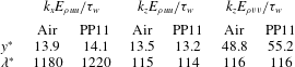
Near-wall turbulent structures can be also analysed by means of the quadrant analysis (Wallace Reference Wallace2016). This representation allows a detailed study of the physical mechanisms producing the Reynolds shear stresses and, in a related way, underlying the turbulent kinetic energy production. The
 $(u,v)$
plane is divided into four quadrants: Q1 (
 $+u^{\prime \prime },+v^{\prime \prime }$
), Q2 (
 $-u^{\prime \prime },+v^{\prime \prime }$
), Q3 (
 $-u^{\prime \prime },-v^{\prime \prime }$
), Q4 (
 $+u^{\prime \prime },-v^{\prime \prime }$
). The contribution of the different quadrants can be obtained by plotting the isocontours of the probability-weighted Reynolds shear stresses
 $\unicode[STIX]{x1D70C}u^{\prime \prime }v^{\prime \prime }/\unicode[STIX]{x1D70F}_{w}P(\sqrt{\unicode[STIX]{x1D70C}}u^{\prime \prime }/\sqrt{\unicode[STIX]{x1D70F}_{w}},\sqrt{\unicode[STIX]{x1D70C}}v^{\prime \prime }/\sqrt{\unicode[STIX]{x1D70F}_{w}})$
, depicted in figure 23. Near the walls probability-weighted Reynolds shear stresses appear stretched in the streamwise direction and flatter in the spanwise direction, with a strong contribution in the Q2 and Q4 quadrants, corresponding respectively to ejections (
 $u^{\prime \prime }<0,v^{\prime \prime }>0$
) and sweeps (
 $u^{\prime \prime }>0,v^{\prime \prime }<0$
). Moving towards the centreline, the contributions become more isotropic. The most important differences between air and PP11 are found in the buffer layer. Namely, the contribution of ejections events to shear stresses appear lower for PP11 flows with respect to air flows. This is consistent with recent findings of Patel et al. (Reference Patel, Peeters, Boersma and Pecnik2015). Gas-like (liquid-like) transport properties tend to stabilize (weaken) the low-speed streaks, which lift less (more) intensely away from the wall.
Probability-weighted Reynolds shear stress
 $\unicode[STIX]{x1D70C}u^{\prime \prime }v^{\prime \prime }/\unicode[STIX]{x1D70F}_{w}P(\sqrt{\unicode[STIX]{x1D70C}}u^{\prime \prime }/\sqrt{\unicode[STIX]{x1D70F}_{w}},\sqrt{\unicode[STIX]{x1D70C}}v^{\prime \prime }/\sqrt{\unicode[STIX]{x1D70F}_{w}})$
for air (a–c) and PP11 (d–f).

6 Conclusions
Direct numerical simulations of supersonic turbulent channel flow of dense gases were carried out by selecting a heavy fluorocarbon, called PP11, as representative of the dense-gas behaviour in the saturated vapour region. This fluid is characterized by an extended range of thermodynamic conditions in the vapour phase such that the fundamental derivative of gas dynamics,
 $\unicode[STIX]{x1D6E4}$
, is lower than one; additionally, this fluid is predicted to exhibit a relatively wide inversion zone. Both features lead to a non-monotonic variation of the speed of sound with density in isentropic perturbations. Another striking point is that, in the dense-gas region, the fluid transport properties depend both on temperature and density. Dense-gas effects on wall turbulence are investigated by means of a parametric study at three bulk Reynolds numbers (namely,
 $Re_{B}=3000$
, 7000 and 12 000) and three bulk Mach numbers (
 $M_{B}=1.5$
, 2.25 and 3). The thermodynamic behaviour of PP11 is well represented by the Martin–Hou thermal equation of state. For comparison, compressible DNS with the same parameters are also carried out for air flows, under the ideal-gas assumption. The main results are as follows.
The analysis of mean and fluctuating thermodynamic and transport properties reveals several peculiarities of wall-bounded dense-gas flows. Primarily, unlike perfect gases where viscous heating leads to high centreline temperatures, in dense-gas flows the high specific heat leads to negligible temperature variations, thus reducing the need for wall cooling. As a consequence the wall behaves as isothermal and (nearly) adiabatic at the same time. Since the temperature is almost constant throughout the flow, variations of the thermodynamic and transport properties are tightly correlated to the fluid density (or pressure). Specifically, speed of sound and viscosity variations are essentially due to the density, which decreases from the walls toward the centreline. On the one hand, this leads to less marked increase of speed of sound at the channel centreline and, subsequently, to centreline Mach numbers greater than the bulk ones, contrary to perfect gases. On the other hand, in the dense-gas region viscosity has an opposite behaviour with respect to the density, and decreases toward the channel centre. As a consequence, compressible dense-gas flows are found to share many features found in variable-property liquids, albeit the driving mechanisms are deeply different (in liquids viscosity decreases due to temperature increasing toward the centreline). This is confirmed by global quantities such as the friction coefficient or the Nusselt number, which are important for industrial purposes. Specifically, the former is well described by a compressible extension of the FIK identity accounting for fluid property variations and follows reasonably well a classical empirical correlation for incompressible flows, unlike perfect gases with exhibit significant Mach number effects. Despite the apparent liquid-like behaviour, supersonic flows of dense gas are characterized by strong compressibility effects. This other facet is highlighted by the distributions of the turbulent Mach number which are similar as those observed for a perfect gas but with slightly higher levels, due to the overall lower speed of sound. Note that, for this confined flows, the maximum values obtained with the considered range of bulk Mach numbers remain below the limit where strong compressibility effects, like eddy shocklets, are visible. Peculiar features of dense gas, such as BZT phenomena where expansion shocks become admissible, are thus not observed. The study of the local value of the derivative of gas dynamics
 $\unicode[STIX]{x1D6E4}$
, which is an indicator of dense-gas effects, indeed showed that the fluid evolves in the dense-gas region (
 $\unicode[STIX]{x1D6E4}<1$
) without taking on negative values, where BZT phenomena can occur. Even without BZT effects, the peculiar behaviour of the speed of sound in dense gases deeply modifies fluctuating density profiles leading to, e.g. maximum r.m.s. levels located close to the channel wall instead of in the buffer layer as in standard compressible channel flows.
This dual behaviour that bears both liquid-like and gas-like features helps to shed some light on the modification of wall turbulence in the presence of a dense gas. As already shown in previous studies for both supersonic channel flows or low-speed variable-property channel flows, the semi-local scaling introduced by Huang et al. (Reference Huang, Coleman and Bradshaw1995), and later formalized by Patel et al. (Reference Patel, Peeters, Boersma and Pecnik2015) or Trettel & Larsson (Reference Trettel and Larsson2016), is well adapted to compare results from existing surveys and with the well-documented incompressible limit. Note that the Van Driest transformation already provides a good collapse for PP11 flows since the heat transfer at the walls is weak. The comparison of second-order statistics and instantaneous views of the velocity fields also gives a strong support for the validity of semi-local scaling with dense-gas flows. Overall, this amounts to saying that Morkovin’s hypothesis is still a good framework for this complex fluid. The fact that the order of magnitude of density and pressure fluctuations is roughly similar to air flows and that a strong reduction of temperature fluctuations is noticed reinforces this conclusion. The structure of turbulence is thus not deeply altered in dense-gas supersonic channel flows. The main effect of variable properties can be taken into account by using the semi-local scaling, revealing the weak coupling between the vortical mode and the mode associated with thermophysical properties. This is exemplified by comparing results with a constant semi-local friction Reynolds number, namely cases AM3R7 and PM1R3 with
 $Re_{\unicode[STIX]{x1D70F},c}^{\ast }\approx 200$
. Some particular features are nonetheless observed with PP11 flows, notably for the highest value of the Mach number,
 $M_{B}=3$
. Furthermore the length scales of near-wall structures have been quantified using premultiplied one-dimensional spectra. The streamwise and spanwise non-dimensional length of the structures are found to be universal with respect to constant property when semi-local coordinates are used. The density field near the wall looks however different because the streaks correspond directly to high- and low-density fluid region for a perfect gas whereas instantaneous density follows pressure fluctuations in PP11 flows, since density fluctuations are now correlated with pressure ones. Additionally, joint-pdfs of streamwise and wall-normal velocity fluctuations reveal that the generation of Reynolds stresses follows the classical picture of wall turbulence when variable properties are included in the semi-local scaling. A slight reduction of ejection events is observed for PP11 flows.
Although non-classical dense-gas effects (like, e.g. unconventional shocklets) are not present in turbulent channel flows, where the turbulent Mach number remains small even for the highest values of
 $M_{B}$
, the present results allow for the first time to shed some light on wall-bounded dense-gas turbulence, for which no experimental data are available, and open the way to the development of numerical models for the prediction of more complex configurations, such as turbine cascades. In particular, information obtained about the appropriate scalings, the behaviour of thermophysical properties, and grid resolution requirements may serve as a reference for justifying some assumptions in turbulence modelling for Reynolds-averaged or large eddy simulations. A priori analyses of turbulence models applied to compressible dense-gas flows are planned as future research.
Additional investigation is ongoing to check if the present conclusions still hold when investigating different operating thermodynamic conditions, retaining the same bulk Mach and Reynolds numbers, or by using other dense-gas fluids, such as refrigerants and siloxanes, for which more accurate and complex equations of state exist. Lastly, the study of turbulent boundary layers and the interactions with shock waves would be a further step to investigate the effects of higher Mach numbers and the modification of shock structure in presence of a dense gas.
Acknowledgement
This work was granted access to the HPC resources of GENCI (Grand Equipement National de Calcul Intensif) under the allocation 7332.
Appendix A. Transport properties for dense gases
Transport properties are generally considered to be dependent only on temperature values. Nevertheless, when
 $1<T/T_{cr}<1.5$
and when
 $p>p_{cr}$
(where
 $(\cdot )_{cr}$
denotes critical quantities), pressure has a strong effect on viscosity and thermal conductivity. This effect is usually taken into account by applying correction factors in the formula used to estimate the dilute-gas properties (i.e. the values of viscosity and thermal conductivity in the ideal-gas limit). In the following, we describe the laws derived by Chung, Lee & Starling (Reference Chung, Lee and Starling1984), Chung et al. (Reference Chung, Ajlan, Lee and Starling1988).
A.1 Dynamic viscosity
The Chapman–Enskog theory describes the integral relations for the transport properties when the interactions between colliding molecules are described by a potential energy function. In general terms, the first-order solution for the dilute gas viscosity can be written as:
 $$\begin{eqnarray}\unicode[STIX]{x1D707}_{0}=\frac{26.69({\mathcal{M}}T)^{1/2}}{\unicode[STIX]{x1D70E}^{2}\unicode[STIX]{x1D6FA}_{v}(T)},\end{eqnarray}$$
where
 ${\mathcal{M}}$
is the molecular weight,
 $T$
the temperature,
 $\unicode[STIX]{x1D6FA}_{v}(T)$
the temperature dependence of the collision integral and
 $\unicode[STIX]{x1D70E}(v_{cr})$
the collision diameter. In the derivation of (A 1),
 $\unicode[STIX]{x1D6FA}_{v}$
is obtained as a function of a dimensionless temperature
 $T^{\ast }$
, defined as (Poling et al.
Reference Poling, Prausnitz, O’Connell and Reid2001):
 $$\begin{eqnarray}T^{\ast }=\frac{k_{B}T}{\unicode[STIX]{x1D716}},\end{eqnarray}$$
where
 $k_{B}$
is Boltzmann’s constant (
 $k_{B}=1.38064852\times 10^{-23}~\text{J}~\text{K}^{-1}$
) and
 $\unicode[STIX]{x1D716}$
is the potential energy parameter. Neufeld, Janzen & Aziz (Reference Neufeld, Janzen and Aziz1972) proposed the following empirical equation:
 $$\begin{eqnarray}\unicode[STIX]{x1D6FA}_{v}=\frac{A}{T^{\ast B}}+\frac{C}{\exp (DT^{\ast })}+\frac{E}{\exp (FT^{\ast })}+GT^{\ast B}\sin (ST^{\ast W}-H),\end{eqnarray}$$
with
 $A=1.16145$
,
 $B=0.14874$
,
 $C=0.52487$
,
 $D=0.77320$
,
 $E=2.16178$
,
 $F=2.43787$
 $G=-6.436\times 10^{-4}$
,
 $H=7.27371$
,
 $S=18.0323$
and
 $W=-0.76830$
.
The method of Chung et al. (Reference Chung, Lee and Starling1984, Reference Chung, Ajlan, Lee and Starling1988) starts from (A 1) with
 $\unicode[STIX]{x1D716}/k_{B}=T_{cr}/1.2593$
and
 $\unicode[STIX]{x1D70E}=0.809v_{cr}^{1/3}$
, where
 $T_{cr}$
and
 $v_{cr}$
are the critical temperature and volume, respectively. Furthermore, they multiply the right-hand side of (A 1) by a factor
 $F_{c}$
in order to account for molecular shapes and polarities of dilute gases. The final result for the dilute-gas viscosity
 $\unicode[STIX]{x1D707}_{0}$
reads:
 $$\begin{eqnarray}\unicode[STIX]{x1D707}_{0}=40.785\frac{F_{c}({\mathcal{M}}T)^{1/2}}{v_{cr}^{2/3}\unicode[STIX]{x1D6FA}_{v}},\end{eqnarray}$$
with
 $$\begin{eqnarray}F_{c}=1-0.2756\unicode[STIX]{x1D714}+0.059035\unicode[STIX]{x1D709}_{r}^{4}+\unicode[STIX]{x1D71B}.\end{eqnarray}$$
In (A 5),
 $\unicode[STIX]{x1D714}$
is the acentric factor,
 $\unicode[STIX]{x1D709}_{r}$
is the reduced dipole moment, and
 $\unicode[STIX]{x1D71B}$
is an empirically determined association parameter to characterize the molecular structure effect of polyatomic molecules, the polar effect, and the hydrogen-bonding effect, respectively. Specifically, the reduced dipole moment
 $\unicode[STIX]{x1D709}_{r}$
reads:
 $$\begin{eqnarray}\unicode[STIX]{x1D709}_{r}=131.3\frac{\unicode[STIX]{x1D709}}{(v_{cr}T_{cr})^{1/2}},\end{eqnarray}$$
whereas the association parameter
 $\unicode[STIX]{x1D71B}$
is (Chung et al.
Reference Chung, Ajlan, Lee and Starling1988):
 $$\begin{eqnarray}\unicode[STIX]{x1D71B}=0.0682+4.704\frac{[\text{number of}~-\text{OH groups}]}{{\mathcal{M}}}.\end{eqnarray}$$
For non-polar fluids, the last two terms of (A 5) become zero.
In order to take into account dense-gas effects, the dense-gas viscosity
 $\unicode[STIX]{x1D707}$
writes:
 $$\begin{eqnarray}\unicode[STIX]{x1D707}=\unicode[STIX]{x1D707}_{k}+\unicode[STIX]{x1D707}_{p}\end{eqnarray}$$
being
 $\unicode[STIX]{x1D707}_{k}$
a modified dilute-gas viscosity and
 $\unicode[STIX]{x1D707}_{p}$
a correction term; specifically,
 $$\begin{eqnarray}\displaystyle & \displaystyle \unicode[STIX]{x1D707}_{k}=\unicode[STIX]{x1D707}_{0}[1/G+A_{6}Y] & \displaystyle\end{eqnarray}$$
 $$\begin{eqnarray}\displaystyle & \displaystyle \unicode[STIX]{x1D707}_{p}=36.44\times 10^{-6}\frac{({\mathcal{M}}T_{cr})^{1/2}}{v_{cr}^{2/3}}A_{7}Y^{2}G\exp [A_{8}+A_{9}(T^{\ast })^{-1}+A_{10}(T^{\ast })^{-2}]. & \displaystyle\end{eqnarray}$$
In (A 9) and (A 10),
 $Y=\unicode[STIX]{x1D70C}v_{cr}/6$
is a density-dependent term,
 $G$
is a nonlinear function written as
 $$\begin{eqnarray}G=\frac{A_{1}[1-\exp (-E_{4}Y)]/Y+A_{2}X\exp (A_{5}Y+A_{3}X)}{A_{1}A_{4}+A_{2}+A_{3}},\quad X=\frac{1-0.5Y}{(1-Y)^{3}},\end{eqnarray}$$
and parameters
 $A_{1}$
–
 $A_{10}$
are linear functions of
 $\unicode[STIX]{x1D714}$
,
 $\unicode[STIX]{x1D709}_{r}$
and
 $\unicode[STIX]{x1D71B}$
:
 $$\begin{eqnarray}A_{i}=a_{0}(i)+a_{1}(i)\unicode[STIX]{x1D714}+a_{2}(i)\unicode[STIX]{x1D709}_{r}^{4}+a_{3}(i)\unicode[STIX]{x1D71B},\quad i\in \{1,\ldots ,10\}.\end{eqnarray}$$
Values for the coefficients
 $a_{0}$
,
 $a_{1}$
,
 $a_{2}$
and
 $a_{3}$
are given in table 7. One should note that at very low densities,
 $Y$
approaches zero,
 $X$
and
 $G$
approach unity and the dense-gas term becomes negligible, with (A 10) reducing to (A 1).
Parameters for evaluating the functions
 $A_{i}$
of (A 12) for the computation of the dense-gas viscosity.
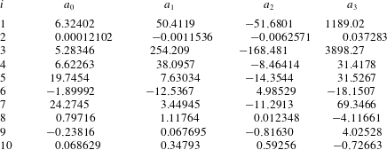
A.2 Thermal conductivity
The dense-gas thermal conductivity is derived, in a similar way, as the sum of a dilute-gas component and a correction term. The dilute-gas component is written as
 $$\begin{eqnarray}\unicode[STIX]{x1D705}_{0}=7.452\frac{\unicode[STIX]{x1D707}_{0}\unicode[STIX]{x1D6F9}}{{\mathcal{M}}},\end{eqnarray}$$
with
 $$\begin{eqnarray}\unicode[STIX]{x1D6F9}=1+\unicode[STIX]{x1D6FC}\frac{0.215+0.28288\unicode[STIX]{x1D6FC}-1.061\unicode[STIX]{x1D6FD}+0.26665\unicode[STIX]{x1D6FF}}{0.6366+\unicode[STIX]{x1D6FD}\unicode[STIX]{x1D6FF}+1.061\unicode[STIX]{x1D6FC}\unicode[STIX]{x1D6FD}}.\end{eqnarray}$$
Here,
 $\unicode[STIX]{x1D6FD}=0.7682-0.7109\unicode[STIX]{x1D714}+1.3168\unicode[STIX]{x1D714}^{2}$
is a fluid-dependent parameter, whereas
 $\unicode[STIX]{x1D6FC}=c_{v,\infty }(T)/R-3/2$
and
 $\unicode[STIX]{x1D6FF}=2+10.5(T/T_{cr})^{2}$
are temperature-dependent functions (
 $c_{v,\infty }(T)$
being the ideal-gas heat capacity at constant volume and
 $R$
the gas constant). The term
 $\unicode[STIX]{x1D6FD}$
is an empirical correlation for the contribution of the internal degrees of freedom of the molecule, and is applied only for non-polar materials. For polar substances
 $\unicode[STIX]{x1D6FD}$
is specific for each compound, and Chung et al. (Reference Chung, Lee and Starling1984) list values for a few materials. If the compound is polar and
 $\unicode[STIX]{x1D6FD}$
is not available, a default value of
 $\unicode[STIX]{x1D6FD}=0.758$
is used. The parameter
 $\unicode[STIX]{x1D6FF}$
represents instead the number of collisions required to interchange a quantum of rotational energy with a quantum translational energy.
The dense-gas thermal conductivity
 $\unicode[STIX]{x1D705}$
is computed by using the same approach as for viscosity:
 $$\begin{eqnarray}\unicode[STIX]{x1D705}=\unicode[STIX]{x1D705}_{k}+\unicode[STIX]{x1D705}_{p},\end{eqnarray}$$
with
 $$\begin{eqnarray}\unicode[STIX]{x1D705}_{k}=\unicode[STIX]{x1D705}_{0}[1/H+B_{6}Y];\quad \unicode[STIX]{x1D705}_{p}=3.039\times 10^{-4}\sqrt{\frac{T}{{\mathcal{M}}}}\frac{1}{v_{cr}^{2/3}}B_{7}Y^{2}H.\end{eqnarray}$$
Again, one has
 $$\begin{eqnarray}\displaystyle \displaystyle Y=\frac{\unicode[STIX]{x1D70C}v_{cr}}{6}; & & \displaystyle\end{eqnarray}$$
 $$\begin{eqnarray}\displaystyle \displaystyle \!\!H=\frac{B_{1}[1-\exp (-B_{4}Y)]/Y+B_{2}X\exp (B_{5}Y+B_{3}X)}{B_{1}B_{4}+B_{2}+B_{3}};\quad X=\frac{1-0.5Y}{(1-Y)^{3}}; & & \displaystyle\end{eqnarray}$$
 $$\begin{eqnarray}\displaystyle & \displaystyle B_{i}=b_{0}(i)+b_{1}(i)\unicode[STIX]{x1D714}+b_{2}(i)\unicode[STIX]{x1D709}_{r}^{4}+b_{3}(i)\unicode[STIX]{x1D71B},\quad i\in \{1,\ldots ,7\}, & \displaystyle\end{eqnarray}$$
with values of
 $b_{0}$
,
 $b_{1}$
,
 $b_{2}$
and
 $b_{3}$
given in table 8.
Parameters for evaluating the functions
 $B_{i}$
of (A 19) for the computation of the dense-gas thermal conductivity.
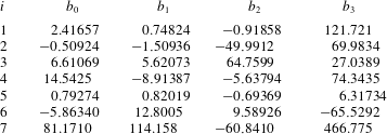
Appendix B. Effect of bulk viscosity
Almost no results are available about the role of the volume or bulk viscosity for turbulent wall-bounded flows of complex molecular fluids, such as the dense gas PP11. Cramer (Reference Cramer2012) showed that some fluids can exhibit bulk viscosities which are hundreds of times larger than their shear viscosities. That is why the assumption used in the present study of a Stokesian fluid, i.e. with a negligible bulk viscosity, is tested for one case, namely PM1R3 (
 $M_{B}=1.5$
,
 $Re_{B}=3000$
) keeping exactly the same parameters (see table 3) but with
 $\unicode[STIX]{x1D707}_{b}=500\unicode[STIX]{x1D707}$
, as defined in § 2.1. We selected a relatively low Reynolds number for cost reasons since the high values of the viscosity induce a further time step restriction for the explicit time marching scheme due to the limitation on the mesh Fourier number. Consequently, the only numerical parameter which is modified is the time step, which is divided approximatively by a factor of fifteen, implying a large number of iterations to achieve convergence of the statistics. The results are presented in figure 24. Second-order statistics such as the Reynolds stresses (figure 24
a) are almost unaffected compared to the simulation with zero bulk viscosity, and the semi-local friction Reynolds number
 $Re_{\unicode[STIX]{x1D70F}}^{\ast }$
changes approximatively
 $0.4\,\%$
, proving that the effects of bulk viscosity are negligible. Cramer & Bahmani (Reference Cramer and Bahmani2014) have recently examined large-Reynolds number flows of fluids having large bulk viscosities. By using the laminar boundary layer equations, they noticed some variations of the thermodynamic pressure across the boundary layer. The distributions of the viscous stresses and of the mean pressure across the channel are investigated in figure 24(b,c), respectively. In the case without bulk viscosity (red lines), the diagonal terms of the viscous stress tensor
 $\overline{\unicode[STIX]{x1D70F}_{ii}}^{+}$
are almost zero, and since in the viscous sublayer
 $\overline{\unicode[STIX]{x1D70C}}\widetilde{v^{\prime \prime }v^{\prime \prime }}\approx 0$
, the pressure remains constant according to (4.4). This is not the case when considering a high value of bulk viscosity, being
 $\overline{\unicode[STIX]{x1D70F}_{ii}}^{+}$
terms as high as 10 % of the wall shear stress close to the walls, causing a decrease of the pressure in the sublayer. Nevertheless,
 $\overline{\unicode[STIX]{x1D70F}_{12}}^{+}$
is almost unchanged with and without bulk viscosity. Additionally, variations of thermodynamic quantities, observed only in the viscous sublayer, are less than 0.5 % and are, therefore, negligible. These results confirm the use of Stokes’ hypothesis in the present DNS study.
Effect of bulk viscosity. (a) Reynolds stresses, (b) viscous stresses, (c)
 $\overline{p}/\overline{p}_{w}$
for case PM1R3. —— (red): no bulk viscosity —— (blue):
 $\unicode[STIX]{x1D707}_{b}/\unicode[STIX]{x1D707}=500$
.

Appendix C. Validations
In order to validate the code and the numerical strategy, two reference test cases have been considered, namely the incompressible channel flow of Kim et al. (Reference Kim, Moin and Moser1987) and supersonic isothermal channel flow of Coleman et al. (Reference Coleman, Kim and Moser1995). The parameters of the DNS are summarized in table 9. Note that a low subsonic Mach number,
 $M_{B}=0.3$
, has been chosen for the comparison of our compressible solver with the incompressible case. Table 10 shows the main results of our simulations. Figure 25 shows the profiles of r.m.s. velocity fluctuations and the evolution of the turbulent kinetic energy budgets compared to the data from Kim et al. (Reference Kim, Moin and Moser1987). Figure 26 shows similar comparison for the first- and second-order statistics for the supersonic case. A very good agreement with the reference results is obtained for both cases.
Parameters used for the DNS of the selected test cases.

Results of the DNS computations.

Validations for the subsonic channel flow case. Lines, present simulation; symbols, data from Kim et al. (Reference Kim, Moin and Moser1987). (a) R.m.s. velocity fluctuations; (b) turbulent kinetic energy budget. In (b), (—
—
—, ▫ red), production; (
 $\boldsymbol{-}\cdot \cdot \boldsymbol{-}\cdot \cdot \boldsymbol{-}\cdot \cdot$
, ▿ orange) dissipation; (
 $\cdots \cdots \cdots \,$
, ▵ green) turbulent diffusion; (- - - - -, ○ blue) viscous diffusion; (
 $\boldsymbol{-}\cdot \boldsymbol{-}\cdot \boldsymbol{-}\cdot \boldsymbol{-}\cdot \boldsymbol{-}\cdot$
, ♢ violet) turbulent pressure diffusion.

Validations for the supersonic channel flow case. Lines, present simulation; symbols, data from Coleman et al. (Reference Coleman, Kim and Moser1995). (a) Profiles of mean quantities; (b) r.m.s. velocity fluctuations.

Appendix D. Grid convergence study
A study of the sensitivity to the grid resolution has been performed for the case
 $M_{B}=1.5$
,
 $Re_{B}=3000$
with both air and PP11 fluids. The resolutions obtained for different grid levels are given in table 11 in semi-local units and normalized by the local Kolmogorov length scale. Figure 27 presents the results for the three components of the Reynolds stresses. At a first glance, we observe that the convergence by refining the grid is faster for air case. This is consistent with the fact that the dense-gas effects yield higher values of the centreline Reynolds number (figure 6). As a consequence, the values of cell sizes expressed in the semi-local coordinates are slightly higher for PP11 cases on a given grid. Nevertheless, the grid convergence analysis shows that the criteria used to select the grid sizes for our study do ensure a clear convergence, so that the results are essentially grid-independent.
Grid resolution in semi-local units and normalized by the Kolmogorov length scale.

Grid convergence study for air (a–c) and PP11 (d–f) for case
 $M_{B}=1.5$
,
 $Re_{B}=3000$
.