1 Introduction
Approximate consensus algorithms are an important building block for many distributed algorithms, including robot formation control (Egerstedt & Hu, Reference Egerstedt and Hu2001), flocking and swarming (Olfati-Saber, Reference Olfati-Saber2006), sensor fusion (Xiao et al., Reference Xiao, Boyd and Lall2005), modular robotics (Yu & Nagpal, Reference Yu and Nagpal2009), and synchronization (Slotine & Wang, Reference Slotine and Wang2005). The current dominant algorithmic approach to distributed approximate consensus is a Laplacian-based approach in which each device finds a weighted local average of its own current value with the values held by its neighbors. In effect, this approach is operating like particle diffusion, such that as the differences between devices eventually equalize, the network is brought into consensus. Although this approach supports a number of elegant mathematical results switching (Olfati-Saber & Murray, Reference Olfati-Saber and Murray2004; Olfati-Saber et al., Reference Olfati-Saber, Fax and Murray2007), including an exponential rate of convergence (derived from the graph Laplacian) toward the mean value of the network, the bounds on the rate of convergence are extremely loose. In reality, many cases of Laplacian-based approximate consensus actually exhibit an extremely slow rate of convergence.
This paper, an extended version of the workshop paper (Beal, Reference Beal2013), investigates the proposition that weakening the requirements for accuracy and resilience can enable algorithms providing great increases in the speed of convergence. In fact, it should be possible to construct an entire spectrum of algorithms allowing an incremental choice of the best possible speed for a given application’s tolerance of decreased accuracy and resilience.
This manuscript begins to populate this spectrum with a new approach to approximate consensus, Power-Law-Driven Consensus (PLD-consensus), based on self-organizing overlay networks. Two algorithms are studied, unidirectional and bidirectional PLD-consensus, both of which converge in O(diameter) time at a cost of increased variability in the converged value. Unidirectional PLD-consensus is fastest and most variable in converged value, while bidirectional PLD-consensus is nearly as fast but with much less variability.
Following a review of approximate consensus and an investigation of hard limits on approximate consensus in Section 2, this manuscript presents the new PLD-consensus approach and the unidirectional and bidirectional algorithms in Section 3. Analysis in Section 4 shows that both PLD-consensus algorithms are expected to converge in O(diameter) time. Section 5 then compares the new algorithms with the Laplacian approach in simulation on spatially distributed networks, a class of networks that appear in many applications (including those listed above) and where Laplacian-based algorithms perform particularly poorly. These experiments confirm that both PLD-consensus algorithms provide drastically faster convergence in spatial networks, and demonstrate the tradeoffs between speed and accuracy across all three algorithms.
2 Approximate consensus challenges and bounds
Consensus is a problem that appears in a wide variety of forms throughout nearly every application in distributed systems. Variants on consensus may be divided into exact and approximate forms. Exact consensus is typically associated with ensuring the integrity of data or transactions, and requires that every non-faulty device select precisely the same decision, often from a finite set of alternatives. There is a long and rich literature on exact consensus (Lynch, Reference Lynch1996), including a great number of impossibility results concerning the impossibility of ensuring both progress and safety in the presence of various classes of fault. Approximate forms of consensus, on the other hand, concern continuous values and are more typically associated with problems of estimation and control. In all cases, consensus algorithms must aim to ensure:
-
∙ Agreement: every device comes to either the same value (exact) or values bounded within some specified difference (approximate);
-
∙ Validity: the agreed values are drawn from the initial set of values (exact) or their convex hull (approximate); and
-
∙ Progress: agreement is achieved within some finite time.
This paper considers approximate consensus algorithms of the following form: given a real-number initial local value l i (0) for each device i, provide a valid estimate of the mean of l i (0) over all devices. These algorithms are closely related to distributed synchronization (e.g. Kuramoto, Reference Kuramoto1984; Mirollo & Strogatz, Reference Mirollo and Strogatz1990), which is approximate consensus on a cyclic number space. Another close relative is gossip-based mean estimation (Mosk-Aoyama & Shah, Reference Mosk-Aoyama and Shah2008; Shah, Reference Shah2009), which provides rapid coarse estimation of means, though it does not attempt to satisfy validity and estimating to within a fixed accuracy requires message size proportional to the square of the mean.
Currently, approximate consensus is generally implemented using a Laplacian-based approach (Olfati-Saber et al., Reference Olfati-Saber, Fax and Murray2007) that computes the approximate mean of l i (0) by iteratively applying the transformation:
 $$l_{i} (t){\,\equals\,}l_{i} (t{\minus}1){\plus}{\epsilon}\mathop{\sum}\limits_{j\,\in{\cal \,N}{\rm (}i{\rm ,}\,t{\rm )}} {w{\rm (}i{\rm ,}\,j{\rm ,}\,t{\rm )} \cdot {\rm (}l_{j} {\rm (}t{\minus}{\rm 1)}{\minus}l_{i} {\rm (}t{\minus}{\rm 1))}} $$
where
 $${\cal N}(i,t)$$
is the set of graph neighbors of device i at time t, w(i, j, t) is the weight given to neighbor j by device i at time t, and the constant ε>0 is the step size of the algorithm. For simplicity, this manuscript gives only the synchronous specification; only minor modification is required for a more general non-synchronized algorithmFootnote
1
. Also without loss of generality, this manuscript considers only cases where all weights are uniformly equal to 1.
Laplacian-based consensus has been proven (Olfati-Saber et al., Reference Olfati-Saber, Fax and Murray2007) to converge toward the mean value of l i (0). Because convergence has been proven to proceed at an exponential rate with respect to the initial range of l i (0), Laplacian-based consensus is often thought of as being ‘fast’, at least in a theoretical sense. In fact, however, the initial range is only one term of the convergence rate. Convergence rate also depends on both the degree and the diameter of the network, and is much more sharply limited by these, with the actual asymptotic bound:
 $$O{\rm (log(}\mathop {{\rm max}}\limits_i {\rm (}l_{i} {\rm (0))}{\minus}\mathop {{\rm min}}\limits_i {\rm (}l_{i} {\rm (0)))} \cdot \mathop {{\rm max}}\limits_i \left| {{\cal N}{\rm (}i{\rm ,}\,t{\rm )}} \right| \cdot diameter^{{\rm 2}} {\rm )}$$
Degree limits convergence because the process of convergence is only stable if the constant ε is no more than
 ${1 \over {\,\mid\,{\cal N}(i,\,t)\,\mid\,}}$
, or in other words the inverse of a device’s number of neighbors. Thus, even for many small-diameter networks, the reality is that convergence must proceed quite slowly. To understand this bound, consider a large network where device i has x neighbors, and one of those neighbors j has no other neighbors and an initial value of l
j
(0)=1, while all other devices have initial value 0. The maximum decrease in value for device j in a single round is
 ${\epsilon}{\equals}{1 \over x}$
in the first round, so it must take at least O(x) rounds to converge to within any specified error of the mean. Generalizing obtains the bound
 $O\left( {{{\rm max}}_i \left| {{\cal N}(i,\,t)} \right|} \right)$
rounds with respect to degree.
This can have severe consequences for convergence time. For example, an Erdos–Renyi random graph with n devices has an expected diameter of O(log n) but a binomial degree distribution (Bollobas, Reference Bollobas2001). This means that the highest degree devices have O((n)1/2) neighbors, which limits
 ${\epsilon}$
⩽
 ${1 \over {\sqrt n }}$
. Thus, the asymptotic bound on stable convergence in such a network must be
 $O\left( {\sqrt n } \right)$
with respect to degree. Small-world graphs following the Watts–Strogatz model (Watts & Strogatz, Reference Watts and Strogatz1998) have the same asymptotic distribution of distance and degree and thus the same bound. Scale-free networks generated following the Barabasi–Albert model (Albert & Barabasi, Reference Albert and Barabasi2002) have even worse properties: they have a slightly sub-logarithmic diameter, but the devices with the highest degree have degree proportional to n, meaning that the graph has an effective convergence time of O(n) with respect to degree with Laplacian-based consensus.
Diameter also limits convergence because the convergence rate depends on the second eigenvalue of the graph Laplacian (Olfati-Saber et al., Reference Olfati-Saber, Fax and Murray2007). This value is very small for high-diameter mesh networks. In fact, in Elhage and Beal (Reference Elhage and Beal2010) the convergence rate of Laplacian-based consensus has been shown to be O(diameter 2) with respect to diameter on spatially distributed networks.
Our investigation in this paper will focus particularly on spatially distributed networks, as approximate consensus algorithms are frequently needed for such systems, yet they are particularly problematic for Laplacian-based consensus. Formally, we consider a class of networks in which a set of n devices are arranged in a graph G={V, E} and also embedded by a position function p: V→M into a Riemannian manifold M with distance function d. Edges are assumed to be bidirectional, to have equal weight, and to not exist for any two vertexes i and j where d(p(i), p(j)) is greater than some threshold. On such networks, as pointed out above, Laplacian-based consensus has a convergence time of O(diameter 2) (Elhage & Beal, Reference Elhage and Beal2010). Worse, it also has a high constant factor due to the restriction on ε caused by the generally large potential number of neighbors.
When there is no correlation in the distribution of values on devices, this does not matter as much, since a rough estimate of global values can be made from locally sampled information. When values are correlated by their location in the network, however, no reasonable estimate of consensus can be made without moving information over long distances. Since spatial computers often have a large diameter and values are often highly correlated with location, Laplacian-based consensus is often inadequate for application needs, and these systems are thus a good case study for developing a spectrum of approximate consensus algorithms, as well as an immediate application area for faster algorithms enabled by weakened requirements for accuracy or resilience.
Laplacian-based consensus, however, is only one possible approach to approximate consensus, albeit one with the highly desirable properties of guaranteed convergence to the mean and of extreme resilience to a wide range of network faults and changes. Might it be possible to improve on the performance of Laplacian-based consensus by degrading resilience or convergence to the mean? Let us consider an approach at the opposite extreme, of maximum speed and minimal resilience. If an arbitrary device is designated as the root of a spanning tree, the mean value can be computed by summing up the spanning tree, then propagating the value back out along the same route that it came. Even the smallest disruption to this process, however, will result in a failure to converge to the mean value or even a failure to converge at all. The spanning-tree approach, however, is extremely fast: in the absence of failures, consensus will be achieved in at most two·diameter rounds. Moreover, the lower bound of O(diameter) is impossible to beat, since consensus cannot be achieved without information moving across the network at least once.
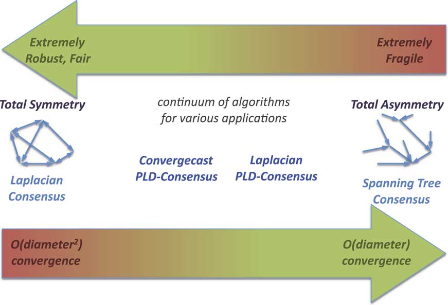
With these two algorithms, we thus have upper and lower bounds on both speed and resilience, with Laplacian-based consensus exhibiting extreme resilience and requiring O(diameter 2) time, while ‘spanning-tree consensus’ is completely non-resilient and requires Θ(diameter) time, quite close to the lower bound of Ω(diameter) time. This implies that there should be a spectrum of possible approximate consensus algorithms filling in the gap between these two extremes, as illustrated in Figure 1. The question is whether algorithms in the middle can provide the best of both worlds, or if they are restricted to provide only the worst of either. We will see, however, through the development of two algorithms based on a new approach to approximate consensus, PLD-consensus, that it is possible to have both speed and resilience. These two algorithms, while both resilient, make different tradeoffs on the matter of speed vs. accuracy in estimating the mean of initial values, and begin the process of filling in the spectrum of approximate consensus algorithms (Table 1).
Approximate consensus is currently generally carried out by Laplacian-based approaches, which are extreme in both their resilience and their slow speed of convergence. An alternate ‘straw-man’ extreme approach is a spanning-tree consensus, which provides a lower bound on time and minimal resilience. This paper proposes that there should exist a spectrum of possible approximate consensus algorithms trading off resilience and/or accuracy for speed, and begins the process of filling in this spectrum with two new algorithms based on Power-Law-Driven Consensus (PLD-consensus), which are both fast and resilient, at the cost of degrading the precision of the converged value to varying degrees

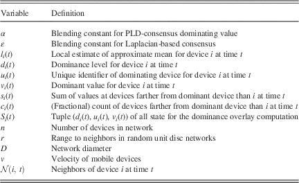
Table of variables

PLD-consensus=Power-Law-Driven Consensus.
3 Power-Law-Driven Consensus
If the problems with Laplacian-based consensus come from the high diameter of the network, then one clear approach to accelerating consensus would be to reduce the effective network diameter through construction of an overlay network containing long-distance links. Since such overlay links may be many hops long, there may be long delays across these links, but that delay is only proportional to the diameter of the network.
PLD-consensus is a simple implementation of such an approach based on a 1/f random distribution, also known as pink noise. Here the 1/f distribution is applied to break symmetry, driving self-organization of the overlay network, by selecting certain devices to have their values spread over a longer distance. Under PLD-consensus, devices compete to become ‘dominant’ over one another, drawing their bids for dominance from the scale-free 1/f distribution. The value of using a scale-free distribution of this sort is that, no matter the size or arrangement of the network, the scale-free distribution ensures that some device will soon draw a bid that is larger enough than the bids of all other devices so that it can dominate the entire network.
Dominance decays over both time and space, so this competition results in a partition of the network into ‘dominance regions’ that shift over time. Values then spread outward from dominant devices through the regions that they dominate, and each device blends the local dominant value with its own value.
Since this distribution is scale free, the regions of dominance begin small. The regions then expand rapidly until the entire network is dominated by a single device, effectively reducing diameter and allowing for rapid convergence. Finally, because dominance decays over time, any dominant device that fails will eventually be replaced by other dominant devices (though this may take a long time).
We will consider two PLD-consensus algorithms, distinguished by the manner in which the values of other devices influence the value of a dominant device. In unidirectional PLD-consensus, the overlay network is used only to carry values from a dominant device to other devices, and is superposed with local blending by Laplacian-based consensus. Thus the value that the network converges to approximate a local mean around the dominant device. Bidirectional PLD-consensus also uses the overlay network to gather a running estimate of the mean value over a device’s region of dominance, and it is this estimated mean that is disseminated as the dominant value. Because of this additional layer of long-distance communication, bidirectional PLD-consensus is slower to converge than unidirectional PLD-consensus, but generally achieves a better estimate of the mean.
3.1 Formal algorithm specification
Having given some intuitions for how PLD-consensus functions, this section now provides a formal specification of the unidirectional and bidirectional PLD-consensus algorithms. For simplicity, this specification will be stated in terms of synchronous rounds. In fact, however, there is no requirement for synchrony: both the overlay construction and blending operations are relaxation methods, meaning that any local updates (within the stable range) are expected to move the system a whole closer to a converged state. The algorithm is thus expected to operate well under a wide range of non-synchronous conditions, and indeed the simulations in Section 5 are non-synchronous.
Let us begin the specification by considering the computation of the dominance overlay. This sub-algorithm serves two functions: first, determining the relative dominance level of each device and second, flowing values down the dominance gradient from more dominant to less dominant devices.
The dominance competition state for each device i at each round t is a tuple S i (t)=(d i (t), u i (t), v i (t)) of the current dominance level d i (t), a unique identifier u i (t) for the current dominant device, and a dominant value v i (t). In addition, each device i has a local value l i (t), which is its current candidate for a consensus value, giving a total state of (S i (t), l i (t)).
At each round, the algorithm considers three candidate states for the new dominance competition state. The driven state S d is:
 $$S_{d} \,{\equals}\,\left( {\left\lfloor {{1 \over {U(0,\,1)}}} \right\rfloor ,\,i,\,l_{i} (t{\minus}1)} \right)$$
where U(0, 1) is a uniform random distribution over the interval (0, 1)Footnote 2 . Taking the inverse of U(0, 1) produces 1/f noise, giving a power-law distribution of candidate new dominance levels being injected into the network at each round.
For each neighbor
 $j\in{\cal N}(i,\,t)$
, where
 ${\cal N}(i,\,t)$
is the set of neighbors of device i at time t, the neighbor-derived candidate state S
j
is:
 $$S_{j} \,{\equals}\,(d_{j} (t{\minus}1){\minus}1,\,u_{j} (t{\minus}1),\,v_{j} (t{\minus}1))$$
which takes the neighbor’s most recent value at a decremented dominance level.
Finally, if no neighbor has a higher dominance level, the leader state S l is:
 $$S_{l} \,{\equals}\,(L_{i} ,\,u_{i} (t{\minus}1),\,l_{i} (t{\minus}1))$$
where the leader dominance L i is
 $$L_{i} \,{\equals}\,\left\{ {_{0}^{{d_{i} (t{\minus}1){\minus}1}} } \right.\,\,_{{else}}^{{if\,\forall j\,\in\,{\cal N}{\rm (}i{\rm ,}\,t{\rm ),}\,d_{i} {\rm (}t{\minus}{\rm 1)\,\gt\,}d_{j} {\rm (}t{\minus}{\rm 1)}}} $$
which decrements the old dominance level and inserts the new local value.
The new state is then set to whichever of these three sources has the highest dominance level:
 $$S_{i} (t)\,{\equals}\,{\rm max}(S_{d} {\cup}S_{l} {\cup}\{ S_{j} \mid j\in{\cal N}(i,\,t)\} )$$
where the maximum is computed lexicographically, such that the first elements of a tuple are compared, then if they are equal the second elements are compared, etc.
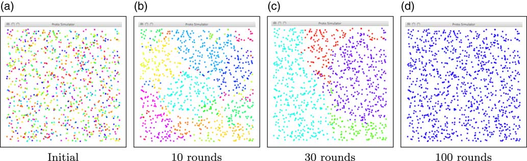
Figure 2 shows an example of the regions of dominance produced by this computation. Initially, no devices are dominant over their neighbors, but as dominance levels are injected via the 1/f noise, regions of dominance grow rapidly until eventually some device is able to dominate the entire network.
Visualization of dominance competition driven by 1/f noise, by having each device spread a unique RGB color. From an initial state where no devices are dominant (a), regions of dominance are expected to grow rapidly (b, c) until eventually some device is able to dominate the entire network (d)

Once the dominance overlay has been established, computation of consensus is relatively straightforward. Given an initial local value of l i (0) at each device i, the value at round t may be computed as a simple proportional blend:
 $$l_{i} (t)\,{\equals}\,\alpha \cdot v_{i} (t){\plus}(1{\minus}\alpha ) \cdot l_{i} (t{\minus}1)$$
where v i (t) is the dominant value as provided from the overlay and α the proportional blending constant. Note, however, that updating in this way uses only overlay values and no neighbor values at all.
Unidirectional and bidirectional PLD-consensus each add non-locality in a different manner. Unidirectional PLD-consensus mixes overlay blending and the local blending of Laplacian-based consensus by the simple expedient of adding the standard Laplacian differential term:
 $$l_{i} (t)\,{\equals}\,\alpha \cdot v_{i} (t){\plus}(1{\minus}\alpha ) \cdot l_{i} (t{\minus}1){\plus}{\epsilon}\mathop{\sum}\limits_{j\,\in\,{\cal N}(i,\,t)} w(i,\,j,\,t) \cdot (l_{j} (t{\minus}1){\minus}l_{i} (t{\minus}1))$$
where ε is the step size for Laplacian-based consensus. PLD-consensus thus makes use of both neighbor values and values delivered through the overlay, and reduces to pure overlay blending when ε=0 and to Laplacian-based consensus when α=0.
Bidirectional PLD-consensus, on the other hand, makes use of the dominance overlay in a second way, to perform a ‘converge-cast’ that sums current values ‘upward’ along the dominance gradient toward the dominant device to compute an estimate of the current overall mean. To do this, each device i maintains a tuple (s i (t), c i (t)) with an estimate of the sum s i of local values and count c i of devices ‘downstream’ of itself away from the dominant device. The device computes this tuple by summing the tuples received from its neighbors in each round, adding its own local value l i , and sending the new total upstream, splitting both values between upstream neighbors. Put formally, a device computes:
 $$(s_{i} (t),\,c_{i} (t))\,{\equals}\,(l_{i} (t),\,1){\plus}\mathop{\sum}\limits_{j\,\in\,{\cal N}(i,\,t)\left| {d_{j} (t{\minus}1)\,\lt\,d_{i} (t{\minus}1)} \right.} \left( {{1 \over {U_{j} (t{\minus}1)}}s_{j} (t{\minus}1),\,{1 \over {U_{j} (t{\minus}1)}}c_{j} (t{\minus}1)} \right)$$
assuming that tuples are added as vectors and where U j (t) is the number of upstream neighbors of device j at time t:
 $$U_{j} (t)\,{\equals}\,\mid\{ k\in{\cal N}(j,\,t) \!\mid \!d_{j} (t)\,\lt\,d_{k} (t)\} \!\mid\,$$
The estimated mean of devices downstream of device i is then s i (t)/c i (t). At a dominant device, this covers the entire network, and this value is taken as the value to be propagated from dominant devices rather than l i (t). Bidirectional PLD-consensus thus acts much like a spanning tree in estimating and broadcasting mean, except that there is more redundancy because there are potentially many paths simultaneously operating both toward and away from its root at the dominant device.
The estimate of the mean computed by bidirectional PLD-consensus will, of course, be lagged and out of date, but nevertheless, as we will see, allows bidirectional PLD-consensus to generally arrive much closer to the true network mean than unidirectional PLD-consensus, since information about device values moves toward a dominant device as fast as the information about the dominant device propagates outward.
4 Analysis
In order to analyze the convergence time for PLD-consensus, let us consider two portions of the algorithm independently. First, we determine the time it takes before some device i comes to dominate the network. More precisely, we aim to determine a bound on the time t at which all devices j are expected to hold the same unique identifier u j (t)=i. We can then determine the time required, once a device i dominates the network, for all other devices to converge to its value.
First, let us consider the criteria for a device i to dominate the network at time t. The intuition here is that, because the distribution of dominance values being generated is heavy-tailed, there is a high probability that some device will generate a value that is much higher than all of the others that have ever been generated.
Dominance decreases by 1 across each hop and time step, so a device i can only dominate the network if it generates a value for d i (t) that is significantly higher than the values that any other device generates, and this situation remains the case for long enough for its identifier to propagate across the network. Thus, in a network of diameter D, device i has the potential to become dominant within D rounds if it is the case that:
 $$\forall _{{j\,\ne\,i}} d_{i} (t)\,\gt\,d_{j} (t){\plus}h(i,\,j)$$
where h(i, j) is the distance in hops from i to j. Let us compute the probability of having such a single value much higher than the rest. The likelihood of such being generated for some device i in the first round in the range D⋅(x+2)⩾d i (t)>D·(x+1) for some integer x, may be bounded below by:
 $$P(round\,1\,x{\minus}high) \,⩾ \,n \cdot P(D(x{\plus}2) \,⩾ \, d_{i} (t)\,\gt\,D(x{\plus}1)) \cdot P(d_{{j\,\ne\,i}} \,⩽ \, Dx)$$
 $$P(round\,1\,x{\minus}high)\,⩾\, n \cdot \left( {{1 \over {D(x{\plus}1)}}{\minus}{1 \over {D(x{\plus}2)}}} \right) \cdot \left( {1{\minus}{1 \over {Dx}}} \right)^{{n{\minus}1}} $$
 $$P(round\,{\rm 1}\,x{\minus}high)\,⩾ \,n \cdot {1 \over {D(x{\plus}1)(x{\plus}2)}} \cdot \left( {1{\minus}{1 \over {Dx}}} \right)^{{n{\minus}1}} $$
Since it takes D rounds for an identifier to propagate across the network, the likelihood that the other devices keep generating lower values for long enough for device i to become dominant is:
 $$P(round\,1\,x{\minus}dominance) \,⩾\, P(round\,1\,x{\minus}high) \cdot \left( {1{\minus}{1 \over {Dx}}} \right)^{{D(n{\minus}1)}} $$
What if the very high value is generated sometime between the first round and some later round Dk, rather than only in the first round? We can bound the likelihood of this event by adding another Dk rounds of lower values and chances for higher values, for an equation of:
 $$P(round\,Dk\,x{\minus}dominance)\,⩾\, n \cdot \left( {1{\minus}\left( {1{\minus}{1 \over {D(x{\plus}1)(x{\plus}2)}}} \right)^{{Dk}} } \right) \cdot \left( {1{\minus}{1 \over {Dx}}} \right)^{{D(n{\minus}1){\plus}Dk(n{\minus}1)}} $$
which may be simplified to the slightly lower bound:
 $$P(round\,Dk\,x{\minus}dominance) \,⩾\, n \cdot \left( {1{\minus}\left( {1{\minus}{1 \over {D(x{\plus}1)(x{\plus}2)}}} \right)^{{Dk}} } \right) \cdot \left( {1{\minus}{1 \over {Dx}}} \right)^{{D(k{\plus}1)n}} $$
Note that two of the exponential terms match the compound interest identity:
 $$\mathop {{\rm lim}}\limits_{D\to\infty} \left( {1{\plus}{a \over D}} \right)^{{bD}} {\equals}\,e^{{ab}} $$
such that as D rises, the probability converges to:
 $$P(round\,Dk\,x{\minus}dominance) \,⩾\, n \cdot \left( {1{\minus}e^{{{\minus}{k \over {(x{\plus}1)(x{\plus}2)}}}} } \right) \cdot e^{{{\minus}{{(k{\plus}1)n} \over x}}} $$
Multiplying through, we obtain the expression:
 $$P(round\,Dk\,x{\minus}dominance) \,⩾\, ne^{{{\minus}{{(k{\plus}1)n} \over x}}} {\minus}ne^{{{\minus}{{(k{\plus}1)n} \over x}{\minus}{k \over {(x{\plus}1)(x{\plus}2)}}}} $$
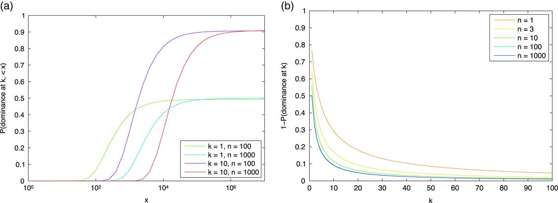
Numerical evaluation shows that for any fixed k and n, the cumulative sum with respect to x forms a sigmoid representing a lower bound on the likelihood of a dominant value (in any range) being generated by round Dk (Figure 3(a)). This value is significant even for k=1 and small n, rising slowly with n and rapidly with k (Figure 3(b)). Overall, the numerical trend is consistent with convergence with high probability in O(D) time.
Numerical evaluation of Equation (21) shows (a) that cumulative probability with respect to x forms a sigmoid representing a lower bound on the likelihood of a dominant value in round Dk, and (b) summing over the range x=1 to 108 for various n and k demonstrates low sensitivity to network size and rapid convergence with k

Once there is a single dominant value in the network, arriving at every device within O(D) rounds, every round it moves every device at least one step toward consensus by blending with that device’s value at rate α. Unlike with Laplacian-based consensus, the value of α is not constrained by neighborhood size, since there is only a single dominant value to blend with. Thus, the network as a whole moves toward consensus exponentially with a time constant of O(D).
It remains only to ensure that feedback to the dominant value is stable. For unidirectional PLD-consensus, this is determined by the ε parameter of Laplacian-based consensus, which is constrained by neighborhood size: as long as this bound is observed, it is impossible for the estimated mean to depart from the initial range of l i (0). For bidirectional PLD-consensus, the inclusion of the weighting term in the converge-cast means that even if values are lost or repeated the estimated mean cannot escape the bounds of the minimum and maximum value in the network.
Note, however, that nothing is guaranteed about the eventual value that either PLD-consensus algorithm will converge to. In either case, it is possible to construct a network and execution pattern so as to ensure that a value arbitrarily far from the mean is chosen. Consider, for example, a network of n devices with a linear topology, where all of the devices are strung out into a single long chain. If one end device has value n and all others have value 0, and dominance emerges in a pattern moving away from the n device, such that it is always blending with incoming zero values, then for the first n rounds it will move toward 0 while all other devices stay at 0. Thus, although the mean value of the network is 1, the consensus value must be less than (1−α) n . In practice, however, we will find that bidirectional PLD-consensus often converges to values close to the true mean.
5 Experimental validation
This section presents experimental validation of the two PLD-consensus algorithms in simulation, providing a quantitative comparison of the tradeoffs between speed and accuracy for these two algorithms vs. Laplacian-based consensus under a range of different configurations and conditions of execution. In particular, Section 5.1 illustrates the convergence dynamics of the various algorithms with a detailed presentation of a single test case. Section 5.2 then quantifies the convergence process, while Section 5.3, 5.4, and 5.5 examine how convergence is affected by network diameter, device mobility, and choice of algorithm parameters, respectively.
These experiments use implementations of both the unidirectional and bidirectional PLD-consensus algorithm in Proto (Beal & Bachrach, Reference Beal and Bachrach2006) (MIT Proto), as well as a Proto implementation of Laplacian-based consensus. The code for all three algorithms is listed in Appendix 1. Proto was a desirable language for implementation and experimental validation for two reasons: first, Proto’s programming model allows a concise and direct implementation of the mathematical specification given in the previous section, and, second, the network simulator distributed with MIT Proto made it simple to run and analyze experiments on large spatially distributed networks.
Except where otherwise noted, all experiments are run with the following parameters: the network consists of 1000 devices distributed uniformly randomly in a 100×100 m rectangle. Devices use a unit disk model of communication, broadcasting to all other devices within r meters, where r is computed to give an expected 10 neighbors per device. The algorithms are run for 1000 rounds of partially synchronous execution, in which all devices execute rounds with equal frequency and randomly offset phase. The PLD-consensus algorithms are run with α=0.02; unidirectional PLD-consensus is run with ε=0, in order to focus investigation on the overlay-based portion of the algorithm’s action. Laplacian-based consensus is run with a step size of ε=0.02. For each experimental condition, 10 trials are run (which is sufficient for comparing behaviors of well-behaved algorithm properties).
The analysis of convergence statistics uses an arbitrary threshold of ‘good-enough’ approximate consensus, since approximate consensus can never achieve a perfect equality of values. In addition, with random graphs and mobile devices some fraction of devices may be disconnected—either mostly or entirely—from the bulk of the network and thus unable to effectively participate in consensus. To exclude the values of such devices from our analysis, the devices with the top and bottom 2.5% of values are ignoredFootnote 3 . A network will thus be considered to have converged if the difference between the minimum and maximum value within the median 95% of devices is <1% of the initial difference (e.g. <0.01 if all devices start with values between 0 and 1).
5.1 Illustrative comparison of algorithms
Let us begin with an illustrative comparison of Laplacian-based consensus and the two PLD-consensus algorithms, to provide an initial intuition of the difference between these approaches.
This experiment uses a set of 1000 devices distributed uniformly randomly in a 400×100 m rectangle. The broadcast communication radius r is chosen to give ~15 expected neighbors per device (r=13.8 m). Devices are initialized to one of two values based on their spatial location, with devices in the left hand side of the plane given an initial value l i (0)=30, and on the right hand side l i (0)=100, producing a highly spatially correlated distribution. To have the purest comparison of PLD-consensus and Laplacian-based consensus, this experiment considers the case of α=0.01 and ε=0 for PLD-consensus, meaning that only dominance overlay values are used, and compares against a step size of ε=0.01 for Laplacian-based consensus.
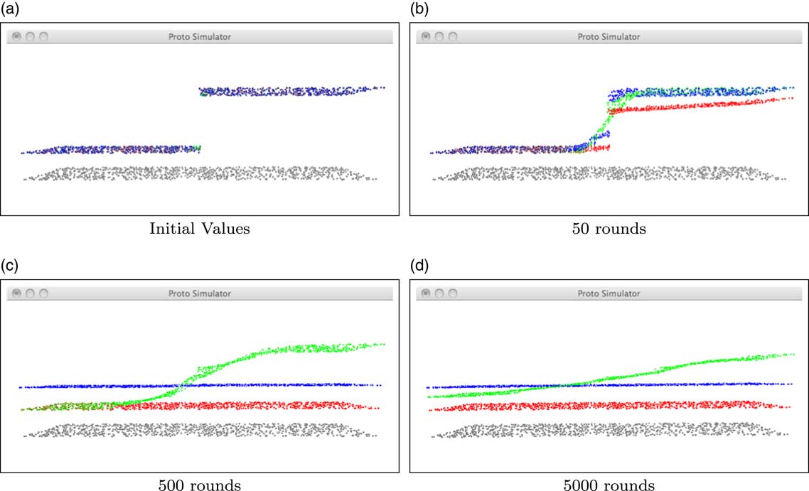
Figure 4 shows the evolution of values held by the various devices over time during a single trial run. Although all three cases begin the same, both PLD-consensus algorithms converge rapidly within a few hundred rounds (the unidirectional significantly faster than the bidirectional), while even after 5000 rounds of computation Laplacian-based consensus is nowhere near convergence, with a difference of 41.5 between the minimum and maximum of the median 95%—more than half of the initial value difference.
Power-Law-Driven Consensus (PLD-consensus) vs. Laplacian-based consensus on a mesh network of 1000 devices with ~15 neighbors each. The devices are shown as gray dots distributed in a plane, viewed at an angle, with their current values for consensus showed as the height of colored dots above the plane: red for unidirectional PLD-consensus, blue for bidirectional PLD-consensus, and green for Laplacian-based consensus. From an initial spatially correlated distribution (a), both unidirectional and bidirectional PLD-consensus begin to converge rapidly (b). Both forms of PLD-consensus converge within a few hundred rounds (c), with bidirectional much closer to the true mean than unidirectional. Laplacian-based consensus is guaranteed to eventually arrive at the true mean, but even after 5000 rounds it is far from converged, retaining more than half of its initial range of values (d)

The tradeoff for the faster convergence of PLD-consensus, however, is a decreased accuracy in finding the overall mean value. In this case, the Laplacian consensus values at t=5000 have a mean of 63.47, which is quite close to the true mean of 63.6 (the mean is slightly shifted from the expected 65 due to the random positioning of devices). The converged value of bidirectional PLD-consensus is somewhat farther off, at 55.27, and unidirectional PLD-consensus has converged to a value of 30.14, which is nearly equal to one of the original extremes.
Although this illustration is only a single example, it nicely illustrates the tradeoff in accuracy vs. speed amongst the three algorithms.
5.2 Convergence rate
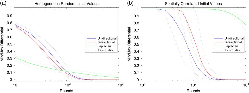
For a more thorough comparison of convergence rate, let us compare the evolution of value distributions in the two PLD-consensus algorithms and Laplacian-based consensus. For this experiment, trials were run for two initial distribution conditions: a homogeneous random condition in which each device’s initial value l i (t) is drawn uniformly randomly from the interval [0, 1], and a spatially correlated condition in which devices in the left half of the distribution start with l i (t)=0 and devices in the right half start with value l i (t)=1. Values were then recorded every 10 rounds for 1000 rounds.
Figure 5 plots the difference between highest and lowest value in the median 95% against time. In both cases, both PLD-consensus algorithms clearly greatly outperform Laplacian-based consensus. Under the homogeneous condition, Laplacian-based consensus initially converges more quickly than either PLD-consensus algorithm, but greatly slows when further convergence requires equalization of values over many hops. With spatially correlated initial values, Laplacian-based consensus has barely even begun to converge by t=1000, and will not complete its convergence for many thousands of rounds more, as seen in the prior illustrative comparison.
Both Power-Law-Driven Consensus (PLD-consensus) algorithms progress toward convergence at similar rates and much faster than Laplacian-based consensus, though Laplacian-based consensus initially progresses more quickly when initial values are homogeneously randomly distributed (a). Unidirectional PLD-consensus converges more quickly than bidirectional when values are spatially correlated (b), but there is a high degree of variance in both

Both PLD-consensus algorithms converge rapidly in both the homogeneous and spatially correlated conditions. Bidirectional PLD-consensus shows much more regularity in its convergence in the homogeneous case, likely due to the fact that in this condition the mean can be approximated well with information from only a few hops distance. In the spatially correlated case, unidirectional progresses significantly faster than bidirectional, due to fact that information only needs to move one way in the overlay network. There is a significant amount of variance in the convergence of both, however, due to the random progress of overlay network construction.
5.3 Scaling with network diameter
The poor scaling of Laplacian-based consensus as network diameter increases has already been demonstrated in Elhage and Beal (Reference Elhage and Beal2010) and discussed above. According to the analysis in Section 4, the time for both PLD-consensus algorithms to converge should be O(diameter), but this analysis did not establish whether the constant on this time is likely to be large or small. The next experiment validates that the O(diameter) estimate is correct, and also shows that the constant is small.
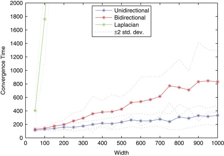
To test this, both PLD-consensus algorithms and Laplacian-based consensus were run for 5000 rounds with spatially correlated initial values on networks with dimensions of X meters width by 20 meters, where the width X ranged from 50 to 1000 m in steps of 50. Devices were distributed at constant density, ranging in number from 125 to 2500. For communication, r was set to provide an expected 20 neighbors (7.14 m)—this higher value was necessary to ensure that such a long thin random network had a high probability of being connected. The diameter of the network thus ranges from at least 7 hops to at least 140 hops. Devices in the left half of the distribution start with l i (t)=0 and devices in the right half start with value l i (t)=1.
For this experiment, convergence of both PLD-consensus algorithms is universal, while Laplacian-based consensus, as expected, is only able to converge within 5000 rounds for the three lowest diameter networks. Figure 6 shows the scaling of convergence time with respect to network width X: as predicted by our analysis, the convergence time of both PLD-consensus algorithms increases approximately linearly with the diameter, atop an approximately constant base convergence time determined by the blending rate. Bidirectional PLD-consensus is, however, significantly slower than unidirectional PLD-consensus.
With spatially correlated distributions, convergence time for both Power-Law-Driven Consensus algorithms increases linearly with the width of the network. Laplacian consensus cannot converge in a reasonable number of rounds except in the smallest of networks

5.4 Scaling with mobility
In many consensus applications, the participating devices are not stationary. This could both be helpful in lowering the effective diameter of the network and problematic in scrambling the structure of the overlay. To investigate the effect of mobility, both PLD-consensus algorithms and Laplacian-based consensus were run with spatially correlated initial values and devices moving at a range of velocities v varying from 0.01 to 2.0 m s−1. Each device moves toward a randomly chosen point in space at velocity v, and upon reaching it (within quantization error) chooses a new point to move toward. Devices in the left half of the distribution start with l i (t)=0 and devices in the right half start with value l i (t)=1. Each trial was run for 2000 rounds.
Two communication radii r were chosen to investigate two qualitatively different mobility scenarios: in the first, r is set to give an expected 10 neighbors (5.6 m), resulting in a network that is generally well connected. In this network, it is almost always possible for values to flow, and the question is whether the overlay is adaptable enough to move them efficiently despite being disrupted by the ongoing changes in neighbor relations. For the second scenario, r is set to given an expected two neighbors (2.5 m), resulting in a network that is generally disconnected into very small components. In this network, values must be ferried to their destinations by the movement of devices, depending on persistence of dominance after the overlay becomes disconnected.
Laplacian-based consensus is known to perform correctly in both cases, though, as usual, it can be very slow to converge. The PLD-consensus algorithms are expected to have two limiting modes of behavior: at low velocities, the overlay should not be disrupted enough to significantly affect the convergence rate. At high enough velocities, the overlay becomes irrelevant, as devices are so well mixed that every device frequently becomes a direct neighbor of the dominant device. At intermediate velocities, however, it is not immediately clear what to expect.
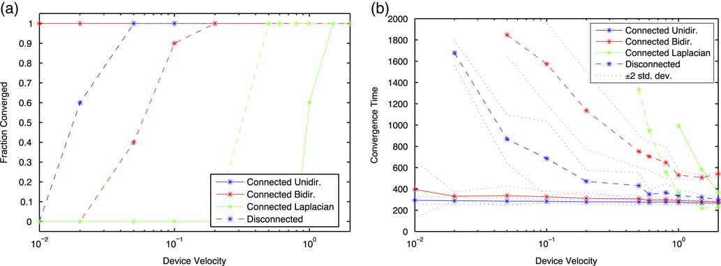
Figure 7 shows the results of this experiment: with the connected network, both PLD-consensus algorithms always converge rapidly for every trial (unidirectional slightly faster than bidirectional, as usual), indicating that the disruptions caused by changes in the overlay network are not a significant problem. In both cases, the convergence time appears to be dominated more by the blending constant α than by the diameter of the network.
When the network is well connected, device mobility has little effect on convergence of either Power-Law-Driven Consensus algorithm. When the network is largely disconnected, however, higher mobility is beneficial: the flexibility of the overlay construction allows values to flow effectively even across gaps in connectivity where they must be ferried by moving devices. Laplacian-based consensus performs poorly except at high velocities, where the motion of devices mixes them well. (a) Percentage converging and (b) time of convergence

With the disconnected network, unidirectional consensus converges much more rapidly than bidirectional consensus. This is likely due to the fact that changes of the members in a connected component can create large perturbations in the mean estimated by converge-cast, but have little effect on broadcast of the dominant value.
Once again, as may be expected, Laplacian-based consensus performs quite poorly in both scenarios, converging within 2000 rounds only for the highest velocities, where the rate at which devices mix is high enough to allow their values to blend rapidly even for Laplacian-based consensus. Surprisingly, Laplacian-based consensus performs better in the disconnected case than the connected case.
5.5 Effect of α and ε parameters
The final experiment considers the effects of the blending parameters α and ε. For both of these parameters, there is a tension between speed and accuracy: the higher they are, the faster the network moves toward convergence, but if they are too high then they will degrade the efficacy of the algorithms. As is well known, when ε is too high, Laplacian-based consensus becomes unstable and values will diverge. When α is too high, there is less opportunity for the dominant value to be brought toward the mean by information flowing from other devices in the network.
To study the effect of varying α, both PLD-consensus algorithms were run with both homogeneous random values and spatially correlated initial values. For the uniform random case, initial values are chosen randomly on the interval [0, 1]; for the spatially correlated case, devices in the left half of the distribution start with l i (t)=0 and devices in the right half start with value l i (t)=1. For these trials, ε=0 and α ranges geometrically from 0.001 to 1.0 at five values per decade, running 30 trials per condition. The experiment for the effect of ε on unidirectional PLD-consensus is the same, except that α=0.02 and ε ranges from 0.001 to 1.0. Finally, for comparison with α variation, Laplacian-based consensus is run with a step size ε that is varied identically.
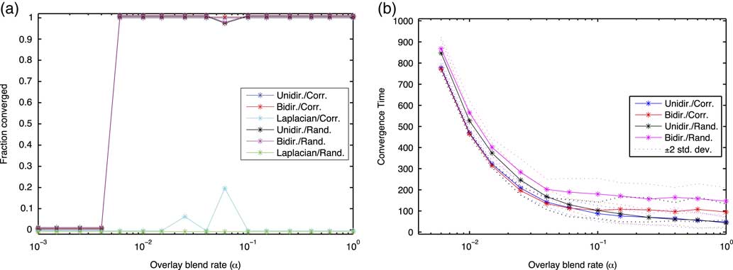
Figure 8 shows the results of varying α. Both PLD-consensus algorithms converge reliably for all but the lowest α. For those trials that converge, the convergence time for low α is close to inversely proportional to α, indicating that convergence is dominated by blend rate. For high α, convergence time is nearly flat, indicating that convergence is dominated by diameter, which regulates overlay construction and the time for values to propagate to and from the dominant device. As expected, once diameter begins to dominate, unidirectional PLD-consensus is significantly faster than bidirectional PLD-consensus. Laplacian-based consensus, on the other hand only converges at all for a few moderate-alpha trials: with low α it converges too slowly and with high α it becomes unstable and values diverge rapidly.
Power-Law-Driven Consensus (PLD-consensus) converges reliably within 1000 rounds for all α⩾0.01 (a): the apparent ‘non-converging’ cases are caused by outlier random graphs with more disconnected devices than usual. Laplacian-based consensus, on the other hand, only barely converges within 1000 rounds for a few trials with intermediate values of ε. Lines are plotted with a small vertical displacement to enhance visibility. For cases where PLD-consensus converges, the convergence time (b) is be dominated by blend rate for low α and by diameter (regulating overlay construction and value relay) for high α

Variation of ε (not shown) produces no significant effect on either the convergence time or on the converged value of unidirectional PLD-consensus, until around ε=0.1, where the Laplacian component becomes unstable and values diverge. These results indicate that the Laplacian component is likely to be operating so slowly on spatially correlated distributions as to have no measurable effect at the diameter studied by this experiment; only at lower α or diameter is there likely to be a significant effect.
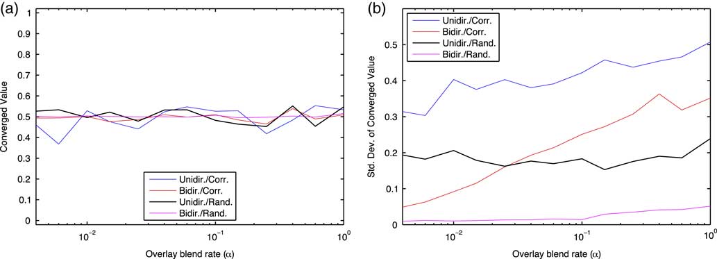
Finally, consider the actual values converged to by the various algorithms. As previously noted, Laplacian-based consensus is guaranteed to converge to the mean value over all devices, once it finally converges. As noted in the analysis in Section 4, however, there can be no similar guarantee for either PLD-consensus algorithm. With a balanced distribution such as those considered in this experiment, however, we may expect that the distribution of converged values to still be centered on the mean, since any device is equally likely to become dominant. Figure 9(a) shows that this is in fact the case in this experiment for all conditions and all values of α. The variation of the mean is another story, and it is here that bidirectional PLD-consensus has a strong advantage over unidirectional. With both correlated and uncorrelated initial values, bidirectional PLD-consensus may be expected to converge much more closely to the mean than unidirectional PLD-consensus. With homogeneous random values, where a good estimate of the overall mean may be taken from the values of nearby devices, bidirectional PLD-consensus performs very well indeed. As the value of α rises, however, there is less opportunity for distant devices to send information about their values toward the dominant device before it is wiped out by the information begin broadcast from there, and the advantage of bidirectional over unidirectional PLD-consensus lessens.
Unlike Laplacian consensus, Power-Law-Driven Consensus (PLD-consensus) will not generally converge to the mean of all initial device values. With a balanced distribution, however, the mean of the converged values over many trials will still likely be close to the true mean, as demonstrated in (a). The standard deviation of converged value (b) depends on how far information can move before a dominant device emerges and drives the system to convergence. Here, bidirectional PLD-consensus always performs much better than unidirectional, since it gathers information more quickly and from farther away. With homogeneous random values, even very short ranges can capture a reasonable approximation of the mean. When values are spatially correlated, higher α results in more variance, as devices move toward a broadcast value before their own inputs can reach a dominant device

6 Contributions and future work
This paper argues that relaxing the requirements for accuracy and resilience in approximate consensus, relative to Laplacian-based consensus, enables a spectrum of algorithms that incrementally tradeoff accuracy and/or resilience for speed. This argument is supported by the introduction of two new approximate consensus algorithms based on self-organizing overlays, unidirectional and bidirectional PLD-consensus. Both operate in O(diameter) time rather than O(diameter 2) for Laplacian-based consensus, with the unidirectional algorithm being faster but likely to be farther from the true mean than the bidirectional algorithm.
No one of these approaches is clearly better than the others. For some applications it may be very important to get a good estimate of the mean: for example, when executing motion planning in modular robotics, approximate consensus can be used to obtain critical physical quantities such as the system’s center of mass. In a case such as this, accuracy of the converged value dominates and Laplacian consensus is likely to be the best approach unless the number of devices in the robot is very large. In other cases, accuracy is less important. For example, when synchronizing transmitters for distributed MIMO, the value arrived at by approximate consensus is fairly unimportant, but it is critical that the consensus be fast and stable. In such a case, unidirectional PLD-consensus can deliver extremely fast convergence. Yet other applications may be in-between and best served by bidirectional PLD-consensus or other intermediate algorithms yet to be discovered.
The work presented in this paper thus makes two contributions. First, it may be applied directly to improve the performance of consensus-based applications for which one of the two PLD-consensus algorithms is appropriate. Second, it forms a basis for investigation of the more general spectrum of approximate consensus algorithms. The PLD-consensus approach sets markers in the ground for one set of tradeoffs. There should exist other algorithms that provide better precision while still improving significantly over the performance of Laplacian-based consensus. Similarly, the PLD-consensus algorithms are designed only for short-term one-shot consensus, and will not work as well for situations where a value needs to be tracked over time or where the dominant device leaves the network and another must take its place. There is a rich space of possible algorithms trading off a number of such factors, and it is to be expected that further investigation in this area will benefit any number of algorithms that depend on approximate consensus phenomena.
Acknowledgments
This work is partially supported by the United States Air Force and DARPA under Contract No. FA8750-10-C-0242. The US Government is authorized to reproduce and distribute reprints for Governmental purposes notwithstanding any copyright notation thereon. The views and conclusions contained herein are those of the authors and should not be interpreted as necessarily representing the official policies or endorsements, either expressed or implied, of DARPA or the US Government.
Appendix 1: Proto code for algorithms
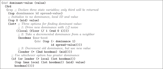
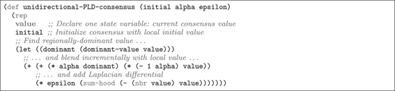
This appendix contains code listings for implementations of all three algorithms examined in this paper: Laplacian-based consensus, unidirectional PLD-consensus, and bidirectional PLD-consensus. Algorithms are implemented in the Proto (Proto Developers, 2005–2014; Beal & Bachrach, Reference Beal and Bachrach2006) spatial computing language. Listings show comments in blue, state variables in green, and Proto keywords in magenta.
Appendix 1.1: Laplacian-based consensus

Appendix 1.2: Unidirectional PLD-consensus
Dominance overlay
Unidirectional PLD-consensus
Appendix 1.3: Bidirectional PLD-Consensus
Dominance overlay: For bidirectional PLD-consensus, two different sets of values move over the same overlay. Thus, rather than computing dominance and moving values down the dominance gradient as a single operation, the algorithm first computes dominance, then independently moves values toward and away from dominant devices.
Estimating mean value upward on dominance gradient

Spreading information outward on dominance gradient

Bidirectional PLD-consensus: Now all of three ingredients are put together to create bidirectional PLD-consensus: computation of the dominance overlay, estimating mean inward on the overlay, broadcasting the estimate outward on the overlay, and blending with the estimate to achieve approximate consensus.