


1. Introduction
The motion of bubbles on a partially wetting substrate is important in application and includes, for example, bubble detachment in nucleate boiling for heat transfer (Douglas et al. Reference Douglas, Boziuk, Smith and Glezer2012; Pereiro et al. Reference Pereiro, Khartchenko, Petrini and Kaigala2019; Ardron & Giustini Reference Ardron and Giustini2021), bubble collapse that affects solder joint quality in ultrasonic-assisted soldering (Shaffer et al. Reference Shaffer, Maassen, Wilson, Tilton, Thompson, Choi and Bostwick2019; Maassen et al. Reference Maassen, Brown, Choi, Thompson and Bostwick2020), bubble detachment via coalescence in catalytic or electrochemical gas evolution reactions in liquids (Lv et al. Reference Lv, Peñas, The, Eijkel, Van Den Berg, Zhang and Lohse2021), microstreaming from oscillating bubbles in micro-electromechanical systems (Marmottant et al. Reference Marmottant, Raven, Gardeniers, Bomer and Hilgenfeldt2006), bubble generation on biological matter (Kawchuk et al. Reference Kawchuk, Fryer, Jaremko, Zeng, Rowe and Thompson2015), and the sound generated by the collapse of a rising bubble at the surface of a lava column (Vergniolle & Brandeis Reference Vergniolle and Brandeis1996). Here, the bubble dynamics may involve translation (detachment), volume change (collapse or growth), liquid/gas surface shape change (oscillations), or some combination thereof, and these are often affected by the wetting conditions on the solid substrate. In this paper, we analyse the canonical case of the sessile bubble by performing a hydrodynamic stability analysis to predict the frequency spectrum, showing how volume and shape-change motions are coupled.
Free spherical bubbles can undergo volume oscillations with frequency (Plesset & Prosperetti Reference Plesset and Prosperetti1977)
 \begin{equation} \omega^2_0= \frac{3\gamma p_{g0}}{\rho R^2}-\frac{2\sigma}{\rho R^3}, \end{equation}
where  $\gamma$ is the adiabatic exponent,
 $p_{g0}$ is the equilibrium gas pressure,
 $R$ is the equilibrium bubble radius, and
 $\sigma$ is the liquid/gas surface tension. Here, the bubble radius
 $r(t)$ is independent of the surface coordinates, and the bubble undergoes pure radial oscillations. Shape-change oscillations of a bubble are a limiting case of the more general Rayleigh–Lamb (RL) spectrum for an immiscible liquid drop when
 $\rho _i=0$ (Rayleigh Reference Rayleigh1879; Lamb Reference Lamb1924):
 \begin{equation} \omega_{k,\ell}^2=\lambda_{k,\ell}^2\,\frac{k(k-1)(k+1)(k+2)}{(k+1)\rho_{i}+k\rho_{e}}\, \frac{\sigma}{R^3}\quad k, \ell=0,1, \ldots,\ \text{and}\ \ell \leq k, \end{equation}
where  $\rho _{i}$ and
 $\rho _{e}$ are the internal and external fluid densities, respectively. Here, the shape-change modes are defined by a polar
 $k$ and azimuthal
 $\ell$ mode number associated with the spherical harmonics
 $Y_k^{\ell }$. Note that the RL spectrum is degenerate with respect to azimuthal mode number
 $\ell$. Extensions to the RL spectrum include, but are not limited to, the effects of (i) a viscoelastic medium (Allen & Roy Reference Allen and Roy2000; Yang & Church Reference Yang and Church2005; Hua & Johnsen Reference Hua and Johnsen2013), (ii) large-amplitude perturbations (Keller & Miksis Reference Keller and Miksis1980; Marmottant et al. Reference Marmottant, Van Der Meer, Emmer, Versluis, De Jong, Hilgenfeldt and Lohse2005), or (iii) constrained geometries (Bostwick & Steen Reference Bostwick and Steen2009; Maksimov & Polovinka Reference Maksimov and Polovinka2013; Anna Reference Anna2016).
Coupling between the purely radial (volume) oscillations and one or more of the shape modes is a vital feature in bubble dynamics, and this has been recognized by researchers since the 1980s. Longuet-Higgins (Reference Longuet-Higgins1989) demonstrated that nonlinear coupling between axisymmetric shape-change modes can induce the volume mode. Mei & Zhou (Reference Mei and Zhou1991) used multiple time scale analysis to study the resonant interactions between an isotropic volume mode and multiple axisymmetric shape-change modes. The review by Feng & Leal (Reference Feng and Leal1997) discusses how the shape-change oscillation amplitude is controlled by nonlinearity, and that energy is exchanged in a continuous, periodic way between the shape-change and volume modes. Notably, Shaw (Reference Shaw2006) considered nonlinear interactions between the axisymmetric shape modes, axial translational motion and volume oscillation of a bubble, with more recent work focused on the effects of viscosity and weak compressibility on the non-spherical gas bubble oscillation (Shaw Reference Shaw2017). Related experiments have been performed by Guédra et al. (Reference Guédra, Cleve, Mauger, Blanc-Benon and Inserra2017, Reference Guédra, Cleve, Mauger and Inserra2020). For the sessile bubble, the coupling between volume and shape-change modes comes from the inherent wetting interactions that are coupled through the free boundary (liquid/gas interface).
The RL spectrum has been used in cases where the bubble is not completely free, as for a levitated bubble (Asaki & Marston Reference Asaki and Marston1995) or a supported bubble (Prosperetti Reference Prosperetti2012; Vejrazka, Vobecka & Tihon Reference Vejrazka, Vobecka and Tihon2013; Maksimov Reference Maksimov2020). Notably, Shklyaev & Straube (Reference Shklyaev and Straube2008) consider both the natural and forced oscillations of a hemispherical bubble with contact-line dynamics prescribed by the Hocking condition (Hocking Reference Hocking1987), which lead to non-trivial interactions between the volume and shape-change modes. Fayzrakhmanova, Straube & Shklyaev (Reference Fayzrakhmanova, Straube and Shklyaev2011) investigated the oscillations of a hemispherical sessile bubble subject to transverse substrate vibrations, focusing on the interplay of the compressibility of the bubble and the contact-angle hysteresis, which leads to stick-slip motions. Bubble oscillations can also be induced by other means, such as electrowetting (Ko, Lee & Kang Reference Ko, Lee and Kang2009) or ultrasonic fields, as seen in experiment (Marin et al. Reference Marin, Rossi, Rallabandi, Wang, Hilgenfeldt and Kähler2015; Volk & Kähler Reference Volk and Kähler2018) and theoretical works (Rallabandi, Wang & Hilgenfeldt Reference Rallabandi, Wang and Hilgenfeldt2014).
Viscous effects enter the bubble dynamics through bulk and boundary layer dissipation that can dampen the bubble oscillations  $\mathrm {e}^{-\gamma t}$, where
 $\gamma$ is the decay rate. Gelderblom et al. (Reference Gelderblom, Zijlstra, van Wijngaarden and Prosperetti2012) contrasted models of viscous potential flow and unsteady Stokes flows to estimate the damping rate for the oscillations of a gas pocket, showing that the latter is a more accurate method, as it includes both boundary layer and bulk dissipation. Wang, Rallabandi & Hilgenfeldt (Reference Wang, Rallabandi and Hilgenfeldt2013) investigated microbubble streaming flows using a matched asymptotic analysis, which included viscous effects in the limit of the thin boundary layer region, and found that axial oscillations could induce fast-decaying flow fields compared to purely azimuthal modes. There is a considerable literature on viscous corrections to the inviscid oscillations of bubble; for example, Vejrazka et al. (Reference Vejrazka, Vobecka and Tihon2013) considered the case of a supported bubble or drop for irrotational flow, using a viscous dissipation approximation that goes back to Lamb (Reference Lamb1924), who predicted the decay rate
 $\gamma =\nu /R^2 (2k+1)(k+2)$, where
 $\nu$ is the kinematic viscosity. For a partially wetting bubble, the problem is complicated by the incompatibility of the no-slip condition with a freely moving contact line, which is resolved typically by introducing a modified Navier slip boundary condition at the solid support. We choose to not focus on these complex issues in our analysis, and instead focus on how the wetting properties affect the oscillation spectrum, by assuming an inviscid fluid in our analysis.
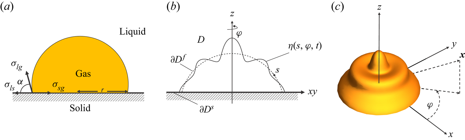
Here, we consider a sessile bubble resting on a planar solid support, as shown in figure 1(a). The wetting interactions are defined by the static contact angle  $\alpha$, as determined by the Young–Dupré equation
 $\sigma \cos \alpha =\sigma _{sg}-\sigma _{ls}$ (Young Reference Young1805; Dupré & Dupré Reference Dupré and Dupré1869). Note that the contact angle
 $\alpha$ convention is defined by the angle measured from the solid through the liquid to the liquid/gas interface. In this case,
 $\alpha <90^\circ$ and
 $\alpha >90^\circ$ correspond to super-hemispherical (drop-like) and sub-hemispherical (lens-like) base states, respectively. Dynamic wetting effects associated with the Hocking condition are neglected, and we assume that the three-phase contact line either (i) moves freely with fixed contact angle (free disturbance), or (ii) is pinned. We note that these are limiting cases of the more general Hocking condition. Finally, we remark that pinned contact-line conditions are generally the more physically relevant boundary condition due to finite contact-angle hysteresis, but that free contact-line motions have been observed recently on slippery liquid-infused porous surfaces (Zhang et al. Reference Zhang, Adera, Aizenberg and Chen2021) and hydrophobic surfaces in microgravity (McCraney et al. Reference McCraney, Kern, Bostwick, Daniel and Steen2022).
Definition sketch. (a) Equilibrium spherical-cap surface of base radius  $r$ and static contact angle
 $\alpha$ defined by the Young–Dupré equation
 $\sigma \cos \alpha =(\sigma _{sg}-\sigma _{ls})$, with interface perturbed by
 $\eta$ in (b) polar cross-sectional and (c) three-dimensional perspective views.

Drops and bubbles are closely related and we note that there has been a lot of recent research on sessile drop oscillations, including theoretical analysis (Bostwick & Steen Reference Bostwick and Steen2014; Sharma & Wilson Reference Sharma and Wilson2021) and experimental observations (Sharp, Farmer & Kelly Reference Sharp, Farmer and Kelly2011; Sharp Reference Sharp2012; Chang et al. Reference Chang, Bostwick, Steen and Daniel2013, Reference Chang, Bostwick, Daniel and Steen2015; Sakakeeny et al. Reference Sakakeeny, Deshpande, Deb, Alvarado and Ling2021). The sessile drop frequency spectra computed by Bostwick & Steen (Reference Bostwick and Steen2014) exhibits a rich structure that includes features such as splitting of the Rayleigh drop degeneracy, spectral reordering and mode mixing, all of which have been verified experimentally. Notably, Steen, Chang & Bostwick (Reference Steen, Chang and Bostwick2019) have produced an organizational structure for the sessile drop spectrum, introducing the ‘periodic table of droplet motions’. In contrast, studies of sessile bubble oscillations are comparably smaller, yet we might expect the dynamics to be somewhat richer given that gas compressibility adds an additional degree of freedom to the dynamics.
We begin this paper by defining the hydrodynamic disturbance equations associated with small disturbances to the spherical-cap–bubble interface, whose three-phase contact line either (i) is pinned or (ii) moves freely with a fixed contact angle. Normal modes are applied to the governing equations, and a boundary integral approach is applied to derive the governing integrodifferential boundary value problem, from which the spectrum is computed by recasting as a functional eigenvalue problem on linear operators. Here, inverse operators are utilized, and a Rayleigh–Ritz procedure is used to reduce the problem to a standard linear algebra eigenvalue problem. Solutions are defined by the mode number pair  $[k,\ell ]$, and we show how the frequency spectrum depends upon the static contact angle
 $\alpha$ and dimensionless equilibrium bubble pressure
 $\varPi$. We report instabilities to the
 $[0,0]$ and
 $[1,1]$ modes, and highlight the respective instability mechanisms. We illustrate how volume and shape-change modes are coupled via the wetting properties, and show how the spectrum splits from the RL spectrum for
 $\alpha \neq 90^\circ$. Finally, some concluding remarks are offered.
2. Mathematical formulation
Consider the sessile bubble, comprised of a compressible, non-condensable gas surrounded by an ambient liquid, shown in figure 1. Under equilibrium conditions and when the effects of gravity are neglected, the liquid/gas interface shape is a spherical cap that can be defined parametrically as
 \begin{equation} \left.\begin{gathered} X(s,\varphi;\alpha)=\frac{\sin(s)}{\sin(\alpha)}\cos(\varphi),\quad Y(s,\varphi;\alpha)=\frac{\sin(s)}{\sin(\alpha)}\sin(\varphi),\\ Z(s,\varphi;\alpha)=\frac{\cos(s)+\cos(\alpha)}{\sin(\alpha)}, \end{gathered}\right\} \end{equation}
using arclength-like  $s \in [0,{\rm \pi} -\alpha ]$ and azimuthal angle
 $\varphi \in [0,2{\rm \pi} ]$ as surface coordinates. The free surface
 \begin{equation} \partial D^{f}\equiv \{ (x,y,z)\,|\,x = X(s,\varphi;\alpha),\ y = Y(s,\varphi;\alpha),\ z = Z(s;\alpha)\} \end{equation}
is endowed with surface tension  $\sigma$ and separates the bubble domain
 \begin{equation} D_{g}\equiv \{ (x,y,z)\,|\, 0 \leq x \leq X(s,\varphi;\alpha), 0 \leq y \leq Y(s,\varphi;\alpha),\ 0 \leq z \leq Z(s;\alpha)\} \end{equation}
from the ambient liquid
 \begin{equation} D_{l}\equiv \{ (x,y,z)\,|\,x \geq X(s,\varphi;\alpha),\ y \geq Y(s,\varphi;\alpha),\ z \geq Z(s;\alpha)\}. \end{equation}
The bubble wets a planar surface-of-support  $\partial D^{s} \equiv \{(x,y,z)\,|\, z=0\}$.
The interface is given a small deformation  $\eta (s,\varphi,t)$, as shown in figures 1(b,c). We will assume that the three-phase contact line either (i) moves freely with fixed contact angle,
 \begin{equation} \frac{{\rm d} \eta}{{\rm d} s}-\cos ({\rm \pi}-\alpha) \eta=0|_{s={\rm \pi}-\alpha}, \end{equation}
or (ii) is pinned,
 \begin{equation} \eta=0 |_{s={\rm \pi}-\alpha}. \end{equation}
2.1. Hydrodynamic field equations
Disturbances to the equilibrium surface induce a capillary-driven flow in the inviscid and incompressible ambient liquid, which can be defined by an irrotational velocity field  $\boldsymbol {v}=\boldsymbol {\nabla } \psi$ using the velocity potential
 $\psi$ that satisfies Laplace's equation on the domain
 $D_l$, a kinematic condition on the free surface
 $\partial D^f$, and the no-penetration condition on the solid support
 $\partial D^s$:
 \begin{equation} \nabla^2 \psi=0 \enspace [D],\quad \frac{\partial \psi}{\partial n}=\frac{\partial \eta}{\partial t}\enspace [\partial D^{f}],\quad \boldsymbol{\nabla}\psi \boldsymbol{\cdot} \boldsymbol{z}=0 \enspace [\partial D^{s}], \end{equation}
with  $\partial /\partial n\equiv \boldsymbol {n}\boldsymbol {\cdot }\boldsymbol {\nabla }$. The pressure field in the liquid is given by the linearized Bernoulli equation
 \begin{equation} p_{l}={-}\varrho\,\frac{\partial \psi}{\partial t} \quad [D], \end{equation}
where  $\varrho$ is the fluid density and
 $p_{l}$ is the pulsation part of the pressure in the liquid phase. The pressure jump across the free surface
 $\partial D^f$ is given by the Young–Laplace equation
 \begin{equation} p_{g}-p_{l}={-}\frac{\sigma}{R^2} \left(2 \eta+\frac{1}{\sin(s)}\,\frac{\partial}{\partial s}\left(\sin(s)\, \frac{\partial \eta}{\partial s}\right)+\frac{1}{\sin^2(s)}\,\frac{\partial^2 \eta}{\partial \phi^2}\right)\quad [\partial D^{f}], \end{equation}
where  $p_{g}$ is the pulsation part of the bubble pressure.
For the bubble, we assume an ideal gas that obeys the adiabatic law
 \begin{equation} [p_{g0}+p_{g}(t)]\,V^{\gamma}(t)=p_{g0}V_{0}^{\gamma}, \end{equation}
where  $\gamma$ is the adiabatic exponent,
 $p_{g0}$ is the equilibrium value of gas pressure, and
 $V_{0}=({{\rm \pi} }/{3})R^3(2+3\cos \alpha -\cos ^3\alpha )$ is the static bubble volume. This assumption implies that the pulsations of the gas pressure in the bubble are spatially homogeneous and the dissipative processes are negligible over a period of oscillation, as described by Shklyaev & Straube (Reference Shklyaev and Straube2008). The instantaneous bubble volume is given by
 \begin{equation} V(t)=V_{0}+{\rm \Delta} V,\quad {\rm \Delta} V=R^2 \int_{\cos({\rm \pi}-\alpha)}^{1} \int_{0}^{2{\rm \pi}}\epsilon\eta\,{{\rm d}x}\,{\rm d}\varphi, \end{equation}
where  ${\textrm {d}x}=\textrm {d}\cos (s)$, and
 ${\rm \Delta} V$ is the linearized volume change. This gives the linearized gas pressure
 \begin{equation} p_{g}={-}\frac{6\gamma p_{g0}}{R(2+3\cos\alpha-\cos^3\alpha)}\int_{-\cos\alpha}^{1} \eta\,{{\rm d}x}. \end{equation}
2.2. Normal-mode reduction
Dimensionless variables are introduced:
 \begin{equation} \rho^{*}=\rho/r, \quad \eta^{*}=\eta/r, \quad t^{*}=t\sqrt{\frac{\sigma}{\varrho r^{3}}},\quad \psi^{*}=\psi \sqrt{\frac{\varrho}{\sigma r}},\quad p^{*}=p\left(\frac{r}{\sigma}\right),\quad \lambda=\omega \sqrt{\frac{\varrho r^3}{\sigma }}, \end{equation}
where  $r$ is the base radius. Normal modes
 \begin{equation} \psi^{*} (\rho,\theta,\varphi, t)=\xi (\rho,\theta)\,{\rm e}^{{\rm i}\lambda t^{*}} \,{\rm e}^{{\rm i}\ell\varphi},\quad \eta^{*}(s,\varphi,t)=y(s)\,{\rm e}^{{\rm i}\lambda t^{*}} {\rm e}^{{\rm i}\ell\varphi}, \end{equation}
are assumed with dimensionless frequency  $\lambda$ and azimuthal mode number
 $\ell$, written in a spherical coordinate system
 $(\rho,\theta,\varphi )$. We apply a boundary integral approach in which (2.7a–c)–(2.9) are mapped to the free surface,
 \begin{align} & \frac{\lambda^2}{\sin^2\alpha}\,\xi +\frac{2\varPi}{\sin\alpha(2+3\cos\alpha-\cos^3\alpha)}\, \delta_{\ell,0}\int_{-\cos\alpha}^{1} \frac{\partial \xi}{\partial n}\,{{\rm d}x} \nonumber\\ &\quad =\left(2-\frac{\ell^2}{\sin^2(s)}\right)\frac{\partial \xi}{\partial n}+ \cot(s) \left(\frac{\partial \xi}{\partial n}\right)' +\left(\frac{\partial \xi}{\partial n}\right)'', \end{align}
where  $\varPi =3\gamma p_{g0} r/\sigma$ is the dimensionless equilibrium bubble pressure,
 $'$ indicates
 $\textrm {d}/\textrm {d} s$, and
 $\delta _{\ell,0}$ is the Kronecker delta with
 $\delta _{0,0}=1,\ \delta _{\ell \neq 0,0}=0$. Here,
 $\xi$ is a harmonic function that solves Laplace's equation on the domain and the no-penetration condition on the surface-of-support.
2.3. Reduction to generalized eigenvalue problem
Equation (2.15) is an integrodifferential eigenvalue problem that can be written in linear operator form as
 \begin{equation} M^{{-}1}[\xi]=\hat{\lambda}^2K^{{-}1}[\xi;\ell],\end{equation}
with  $\hat {\lambda }\equiv \lambda /\sin \alpha$,
 \begin{equation} M^{{-}1}[\xi]=\frac{\partial \xi}{\partial n} -\frac{2\varPi}{\sin\alpha(2+3\cos\alpha-\cos^3\alpha)}\, \delta_{\ell,0}\int_{-\cos\alpha}^{1} \frac{\partial \xi}{\partial n} (y)\,{{\rm d}y} \int_{-\cos\alpha}^{1} G(x,y;\ell)\,{{\rm d}y}\end{equation}
and
 \begin{equation} K^{{-}1}[\xi;\ell]=\int_{-\cos\alpha}^{1}G(x,y;\ell)\,\xi(y)\,{{\rm d}y}. \end{equation}
Here,  $G(x,y;\ell )$ is the Green's function or fundamental solution of the differential operator (right-hand side of (2.15)).
2.4. Green's function
We use the following representation of the Green's function:
 \begin{equation} G(x,y;\ell) = \left\{\begin{array}{ll} \displaystyle\dfrac{1}{1-y^2}\,\dfrac{U(x;\ell)\,V(y;\ell)}{W(y;\ell)}, & b< y< x<1, \\[6pt] \displaystyle\dfrac{1}{1-y^2}\,\dfrac{U(y;\ell)\,V(x;\ell)}{W(y;\ell)}, & b< x< y<1, \end{array}\right. \end{equation}
where  $x \equiv \cos (s)$ and
 $b \equiv \cos ({\rm \pi} -\alpha )=-\cos \alpha$. Here,
 $U$ and
 $V$ are the homogeneous solutions of the curvature operator
 $K$ that satisfy the left-hand and right-hand boundary conditions, respectively,
 \begin{equation} U=y_{1}(x;\ell),\quad V=y_{2}(x;\ell)-\frac{\tau_{2}(\ell)}{\tau_{1}(\ell)}\,y_{1}(x;\ell), \end{equation}
and  $W$ is the Wronskian of the solutions
 $U$ and
 $V$. Also,
 \begin{align} \left.\begin{gathered} y_{1}(x;0)=P_{1}(x),\quad y_{2}(x;0)=Q_{1}(x),\quad y_{1}(x;1)=P_{1}^1(x),\quad y_{2}(x;1)=Q_{1}^1(x),\\ y_{1}(x;\ell\geq2)=(x+\ell)\left(\frac{1-x}{1+x}\right)^{\ell/2},\quad y_{2}(x;\ell\geq2)=\frac{x-\ell}{2\ell(\ell^2-1)}\left(\frac{1+x}{1-x}\right)^{\ell/2}, \end{gathered}\right\} \end{align}
where  $P_{1}$,
 $Q_{1}$ and
 $P_{1}^1$,
 $Q_{1}^1$ are the associated Legendre functions, and the parameters
 $\tau _{1}$ and
 $\tau _{2}$ are related to the contact-line boundary conditions:
 \begin{equation} \tau_{1}^{p}=y_{1}(b;\ell),\quad \tau_{2}^{p}=y_{2}(b;\ell)\end{equation}
for the pinned contact-line disturbance (superscript  $p$), and
 \begin{equation} \tau_{1}^{f}=y_{1}'(b;\ell)+\frac{b}{\sqrt{1-b^2}}\,y_{1}(b;\ell),\quad \tau_{2}^{f}=y_{2}'(b;\ell)+\frac{b}{\sqrt{1-b^2}}\,y_{2}(b;\ell)\end{equation}
for the fixed-angle disturbance, sometimes referred to as the free disturbance (superscript  $f$).
2.5. Solution of the generalized eigenvalue problem
We use a Rayleigh–Ritz procedure to compute the eigenvalue spectrum of
 \begin{align} & \frac{\partial \xi}{\partial n}(x) -\frac{2\varPi}{\sin\alpha(2+3\cos\alpha-\cos^3\alpha)}\, \delta_{\ell,0}\int_{b}^{1} \frac{\partial \xi}{\partial n} (y)\,{{\rm d}y} \int_{b}^{1} G(x,y;\ell)\,{{\rm d}y} \nonumber\\ &\quad =\hat{\lambda}^2\int_{b}^{1} G(x,y;\ell)\,\xi(y)\,{{\rm d}y} \end{align}
from a truncated set of linear algebraic equations that result from minimization of the functional
 \begin{equation} \hat{\lambda}^2=\frac{(M^{{-}1}[\xi],\xi)}{(K^{{-}1}[\xi;\ell],\xi)},\quad \xi \in S,\end{equation}
over a predetermined function space  $S$, which is chosen to satisfy Laplace's equation and the no-penetration condition on
 $\partial D^s$.
We begin by assuming a solution series
 \begin{equation} \xi=\sum_{j=0}^{N}a_{j}\,\xi_{j}^{(\ell)}(\rho,\theta)\end{equation}
constructed from basis functions  $\xi _{j}^{\ell }(\rho,\theta )$. These functions are applied to (2.24), evaluated on the undisturbed surface (2.1a–c), and inner products are taken to generate a set of linear algebraic equations
 \begin{equation} \sum_{j=0}^{N}(m_{ij}^{(\ell)}-\hat{\lambda}^2k_{ij}^{(\ell)})a_{j}=0,\end{equation}
with
 \begin{align} m_{ij}^{(\ell)} &=\int_{b}^{1}\left(\frac{\partial \xi_{i}^{(\ell)}}{\partial n} -\frac{2\varPi}{\sin\alpha(2+3\cos\alpha-\cos^3\alpha)}\,\delta_{\ell,0} \right.\nonumber\\ &\quad \times\left.\int_{b}^{1}\frac{\partial \xi_i^{(\ell)}}{\partial n} (\kern0.7pt y)\,{{\rm d}y} \int_{b}^{1} G(x,y;\ell)\,{{\rm d}y}\right)\xi_{j}^{(\ell)}\,{{\rm d}x} \end{align}
and
 \begin{equation} k_{ij}^{(\ell)}=\int_{b}^{1}\int_{b}^{1}G(x,y;\ell)\,\xi_{i}^{(\ell)}\xi_{j}^{(\ell)}\,{\rm d} x\,{\rm d} y.\end{equation}
Allowable solutions of the generalized eigenvalue problem (2.24) must satisfy Laplace's equation  $\nabla ^2 \xi =0$, and this can be accomplished through proper selection of the basis functions (e.g. Prosperetti Reference Prosperetti2011)
 \begin{equation} \xi_{j}^{(\ell)}(\rho,\theta)=\rho^{{-}j-1}\,P_{j}^{\ell}(\cos\theta),\end{equation}
written here in spherical coordinates,  $\rho$ and
 $\theta$, and chosen to be harmonic. Here,
 $P_{j}^{\ell }$ is the Legendre function of degree
 $j$ and order
 $\ell$, with
 $j+\ell =\mathbb {Z}^{+}_{even}$ to ensure that the no-penetration condition is satisfied. Additionally, a consistency condition requires
 $\ell \leq j$ in order to make sure that the Legendre function is non-singular at
 $\cos \theta =\pm 1$.
For reference, the normal derivatives of the basis function (2.30), evaluated on the equilibrium surface  $(X(s),Y(s),Z(s))$ as defined in (2.1a–c), are expressed as
 \begin{align} \frac{\partial\xi_{j}^{(\ell)}}{\partial n} &= \boldsymbol{\nabla}\xi_{j}^{(\ell)}\boldsymbol{\cdot} \boldsymbol{n}=({-}j-1)\,P_{j}^{\ell}(\cos\theta)\,(\sin s \sin\theta+\cos s \cos\theta)\rho^{{-}j-2} \nonumber\\ &\quad +\sin\theta \left(P_{j}^{\ell}(\cos\theta) \right)'(\sin s \cos\theta-\cos s, \sin\theta)\rho^{{-}j-2} \end{align}
using mixed coordinates for efficiency in presentation.
3. Results
The eigenvalues  $\lambda _{k,\ell }$ of (2.27) have been computed using a resolution of
 $N=10$ basis functions in the solution series (2.26) for both free and pinned disturbances. This produces relative eigenvalue convergence of
 $0.0064\,\%$ for the first five modes. The eigenfunction
 $\xi _{k,\ell }$ associated with the eigenvalue/eigenvector pair
 $\lambda _{k,\ell }$,
 $a_{j}^{(k,\ell )}$ is given by
 \begin{equation} \xi_{k,\ell}(x)=\sum_{j=0}^{N}a_{j}^{(k,\ell)}\,\xi_{j}^{(\ell)}(x),\end{equation}
with corresponding interface deformation
 \begin{equation} y_{k,\ell}(x)=\sum_{j=0}^{N}a_{j}^{(k,\ell)}\, \frac{\partial \xi_{j}^{(\ell)}}{\partial n}(x).\end{equation}
Here,  $k$ indexes the eigenvalues and can be viewed as a polar mode number.
3.1. Mode-shape terminology
Mode shapes can be classified by their mode number pair  $[k,\ell ]$ into zonal
 $[k,0]$, lateral
 $[k,1]$, sectoral
 $[k,k]$, and tesseral
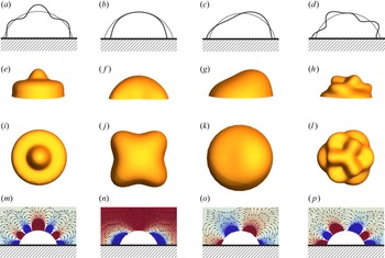
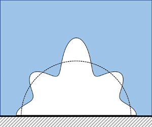
 $[k,\ell \neq k]$, using spherical harmonic terminology (MacRobert Reference MacRobert1967). Figure 2 shows typical mode shapes (perspective view and top view) with corresponding gradient fields (streamlines and pressure field) for a sub-hemispherical bubble (
 $\alpha =105^\circ$) with free disturbance. Zonal
 $\ell =0$ modes are axisymmetric and have a polar mode number
 $k$ that can be determined by the number of intersections of the disturbed and undisturbed shapes, which occur along latitudinal lines. Sectoral
 $k=\ell$ modes have only longitudinal crossings and can be decomposed into
 $k$ symmetric sectors. Tesseral modes
 $k\neq \ell$ have both latitudinal and longitudinal crossings. Lateral
 $\ell =1$ modes are unique in that their motion is predominantly horizontal or side-to-side within the plane of the substrate. Here, we note that sectoral modes display primarily horizontal motions, while zonal modes have strongly vertical motions. Chang et al. (Reference Chang, Bostwick, Steen and Daniel2013) have introduced an alternative classification scheme based on ‘layers’
 $n$ and ‘sectors’
 $\ell$, with
 $n=(k-\ell )/2+1$, that is useful for identifying drop modes in experiment. For example, the mode
 $[3,1]$ has one sector and two layers, yielding
 $(n,\ell )=(2,1)$. Sectoral modes have one layer,
 $n=1$, and zonal modes have zero sectors,
 $\ell =0$.
Mode shape  $[k,\ell ]$ classification plotting the interface shape in two-dimensional polar view (a–d), and three-dimensional side (e–h) and top (i–l) views, with associated fields (m–p, streamlines and pressure contours) for typical (a,e,i,m) zonal
 $[6,0]$, (b,f,j,n) sectoral
 $[4,4]$, (c,g,k,o) lateral
 $[3,1]$, and (d,h,l,p) tesseral
 $[7,3]$ modes, for
 $\alpha =105^\circ$.

3.2. Zonal ( $\ell =0$) modes

3.2.1. Breathing mode ($[0,0]$)

The  $[0,0]$ breathing mode is the only mode that exhibits instability
 $\lambda ^2<0$ for both free and pinned disturbances, with
 $\varPi =0$ being the most unstable case. For each
 $\alpha$, there is a range of values of
 $\varPi$ that gives rise to instability, with the boundary between stability and instability defined by
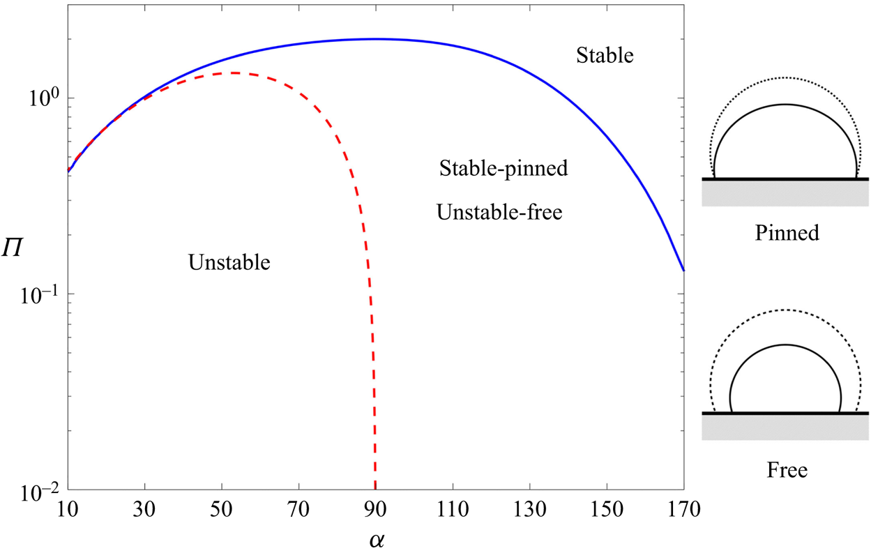
 $\lambda ^2_{0,0}=0$. Figure 3 plots the stability diagram for the breathing mode in the
 $\alpha - \varPi$ parameter space (with typical instability mode shapes inset). Here, instability corresponds to bubble collapse. Increasing the equilibrium bubble pressure
 $\varPi$ can stabilize this collapse. The instability window for the pinned disturbance is smaller than that for the free disturbance, implying that pinning the contact line (i.e. restricting motion) has a stabilizing effect (cf. figure 3). This is also seen in vertical liquid bridges (columns) (Vogel Reference Vogel1982; Bostwick & Steen Reference Bostwick and Steen2010; Benilov & Cummins Reference Benilov and Cummins2013). The free mode is unstable for all
 $\alpha$ (figure 3), whereas the pinned mode is unstable for super-hemispherical
 $\alpha <90^\circ$ base states (figure 3). The latter is related to the pressure turning point in the pressure–volume response curve for a pinned spherical-cap shape (Bostwick & Steen Reference Bostwick and Steen2015, figure 1c).
Stability diagram for the  $[0,0]$ mode, plotting equilibrium bubble pressure
 $\varPi$ against contact angle
 $\alpha$ for free and pinned disturbances, separating stable and unstable regions. Typical instability mode shapes are inset.

Insight into the instability mechanism for the  $[0,0]$ breathing mode can gained by evaluating the disturbance potential energy
 $F$ for the mode shape
 $y_{0,0}$:
 \begin{equation} F=U_{i}+U_{g}=\sigma_{lg} A_{lg}+\sigma_{ls}A_{ls}+\sigma_{sg}A_{sg}-P_{g}\,{\rm \Delta} V, \end{equation}
where  $U_i$ is the interfacial energy,
 \begin{equation} U_{i}=\sigma_{lg} A_{lg}+\sigma_{ls}A_{ls}+\sigma_{sg}A_{sg}, \end{equation}
and  $U_g$ is the potential energy of the gas phase, or work done by the gas pressure on the ambient liquid,
 \begin{equation} U_{g}={-}P_{g}\,{\rm \Delta} V. \end{equation}
Given that the spherical cap is an equilibrium surface, the first variation of energy  $\delta F=0$, and the second variation
 $\delta ^2 F$, will provide information about stability:
 $\delta ^2 F>0$ for stability, and
 $\delta ^2 F<0$ for instability. The second variation of potential energy (3.3) can be written in non-dimensional form as
 \begin{equation} \delta^2 F={-}\int_{b}^{1}\left[ ((1-x^2)y')'+2y\right]y\,{\rm d} x + \frac{2 \varPi}{\sin\alpha(2+3\cos\alpha-\cos^3\alpha)}\int_{b}^{1} y\,{{\rm d}x} \int_{b}^{1} y\,{\rm d} x, \end{equation}
which we can decompose as
 \begin{equation} E_{t}=E_{1}+E_{2},\end{equation}
where the interfacial energy is
 \begin{equation} E_{1}={-}\int_{b}^{1}\left[ ((1-x^2)y')'+2y\right]y\,{\rm d} x, \end{equation}
and the gas pressure energy is
 \begin{equation} E_{2}=\frac{2 \varPi}{\sin\alpha(2+3\cos\alpha-\cos^3\alpha)} \left(\int_{b}^{1} y\,{{\rm d}x}\right)^2.\end{equation}
Here,  $E_2$ is positive definite, and the effect of equilibrium gas pressure
 $\varPi$ is stabilizing, whereas the interfacial energy
 $E_1$ is destabilizing. The instability lowers energy by reducing interfacial area, which can be suppressed by a sufficiently high gas pressure
 $\varPi$.
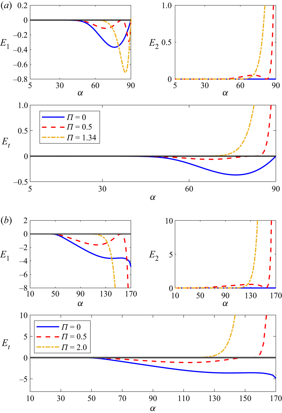
Figure 4 plots the total  $E_t$, interfacial
 $E_1$, and gas
 $E_2$ energies against contact angle
 $\alpha$, as it depends upon the equilibrium pressure
 $\varPi$. Here, states with
 $E_t<0$ are unstable. For pinned disturbances (cf. figure 4a), the super-hemispherical
 $\alpha <90^\circ$ base states are unstable for a range of
 $\varPi$ values provided that
 $\varPi <1.34$, whereas all the sub-hemispherical
 $\alpha >90^\circ$ base states are stable, irrespective of
 $\varPi$. For the free disturbance (cf. figure 4b), all base states can be unstable provided that
 $\varPi <2$. For both pinned and free disturbances, the instability mechanism is the same; energy is lowered by decreasing interfacial area, and it happens that free disturbances are more efficient at decreasing this area, i.e. have a larger instability window, as shown in figure 3.
Energy decomposition for the  $[0,0]$ mode plotting the interfacial energy
 $E_{1}$, gas energy
 $E_{2}$, and total energy
 $E_{t}$, for (a) pinned and (b) free disturbances, against contact angle
 $\alpha$.

3.2.2. Shape-change zonal modes $[k\neq 0,0]$

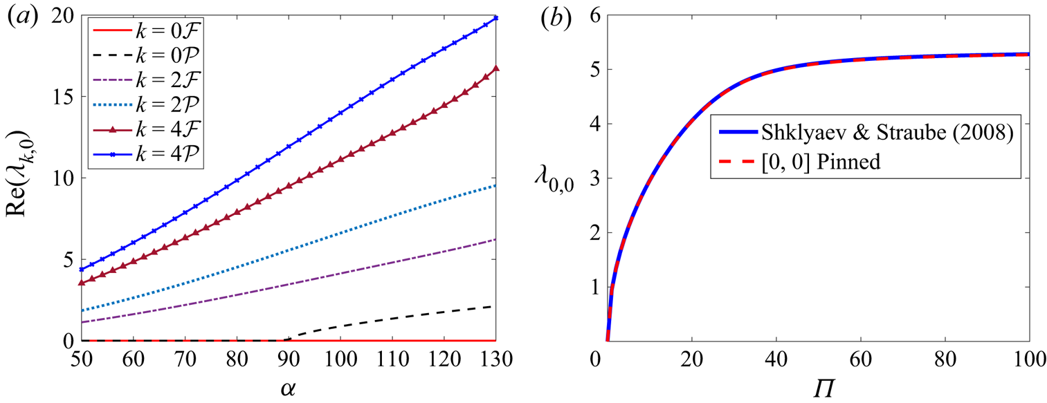
Figure 5(a) plots the zonal frequencies  $\textrm {Re}(\lambda _{k,0})$ against the contact angle
 $\alpha$ for the limiting case
 $\varPi =0$, contrasting the free (
 $\mathcal {F}$) and pinned (
 $\mathcal {P}$) modes. For fixed mode number
 $[k,0]$, the pinned frequencies are always larger than the free frequencies. Increasing
 $\varPi$ is stabilizing (i.e. increases the frequency), as shown in figure 5(b), which plots the
 $[0,0]$ pinned frequency against
 $\varPi$ for the hemispherical
 $\alpha =90^\circ$ base state. This special case has been investigated previously by Shklyaev & Straube (Reference Shklyaev and Straube2008), and our computations reproduce those results.
Zonal  $\ell =0$ modes. (a) Frequency
 $\textrm {Re}(\lambda _{k,0})$ against contact angle
 $\alpha$ for
 $\varPi =0$, contrasting free (
 $\mathcal {F}$) and pinned (
 $\mathcal {P}$) disturbances. Here, the
 $[0,0]$ free mode is unstable (
 $\lambda ^2<0$) for all
 $\alpha$, and the pinned mode for
 $\alpha <90^\circ$. (b) Breathing mode
 $[0,0]$ frequency
 $\lambda _{0,0}$ for the hemispherical
 $\alpha =90^\circ$ base state against equilibrium bubble pressure
 $\varPi$ compared with predictions of Shklyaev & Straube (Reference Shklyaev and Straube2008).

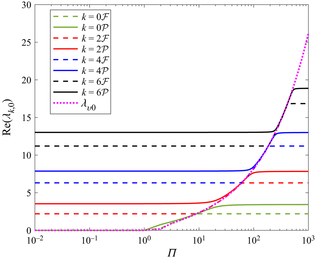
Recall that the zonal  $\ell =0$ modes are the only modes in which the bubble volume changes. The partitioning of that excess volume amongst the modes is interesting. Figure 6 plots the oscillation frequency
 $\textrm {Re}(\lambda _{k,0})$ against
 $\varPi$ for
 $\alpha =70^\circ$, contrasting free and pinned disturbances. For each mode, there are a low-frequency plateau region and a high-frequency plateau region separated by a region where the frequency grows rapidly. Interestingly, these regions of rapid growth form a singular curve related to the volume oscillation mode
 $\lambda _{v0}$, which for a free spherical bubble was given by Plesset & Prosperetti (Reference Plesset and Prosperetti1977) as
 $\omega ^2=\varPi -2$. For contact angles
 $\alpha \neq 90^\circ$, we can estimate
 $\lambda _{v0}$ by using only one term
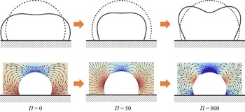
 $N=1$ in our expansion (2.27), which by construction should encompass the volume oscillations of the sessile bubble. This highlights the interaction between the volume and shape-change modes for the sessile bubble, as shown in figure 7, which plots the mode shapes and flow fields as these curves are traversed by increasing
 $\varPi$ from the low-frequency plateau through the rapid-growth region into the high-frequency plateau region. Here, it is clear that volume change occurs within the rapid-growth region, as seen by comparing the mode shapes for varying
 $\varPi$ with fixed
 $[k,0]$. In addition, the mode has changed its spatial character from the low-frequency plateau to the high-frequency plateau by adding a node or increasing its mode number
 $k$. In both plateau regions, volume is conserved through the bubble oscillation. For example, the
 $[2,0]$ mode at
 $\varPi =0$ has the expected spatial structure, but at
 $\varPi =800$ it has the spatial structure of a
 $[4,0]$ mode, despite the fact that it is still the second smallest numerical eigenvalue. That is, there can be some discrepancy in the classical definitions of modal ordering of (i) numerical ordering of eigenvalues, or (ii) nodal (zeros) structure of the eigenmodes. Typically, these definitions are equivalent, but in this case they are not.
Zonal mode frequency  $\textrm {Re}(\lambda _{k,0})$ against equilibrium bubble pressure
 $\varPi$ for
 $\alpha =70^\circ$, contrasting pinned (
 $\mathcal {P}$) and free (
 $\mathcal {F}$) disturbances. For each
 $k$ (pinned or free), there are two plateaus separated by an increasing region where volume change occurs, as related to
 $\lambda _v$. Here,
 $\textrm {Im}(\lambda )=0$ except for the range of
 $\varPi$ where the pinned and free
 $[0,0]$ modes are unstable.

Variation in mode shape and gradient field (streamlines and velocity potential) with increasing  $\varPi$ for the
 $[2,0]$ free mode with
 $\alpha =70^\circ$.

3.3. Lateral $(\ell =1)$ modes

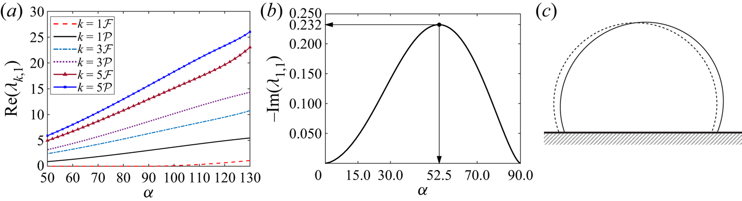
Figure 8(a) plots the oscillation frequency  $\textrm {Re}(\lambda _{k,1})$ for the lateral modes
 $\ell =1$ against the contact angle
 $\alpha$, contrasting free (
 $\mathcal {F}$) and pinned (
 $\mathcal {P}$) disturbances. Here all modes are stable (
 $\lambda ^2>0$) with the exception of the
 $[1,1]$ free mode for super-hemispherical
 $\alpha <90^\circ$ base states. Recall that for
 $\ell \neq 0$, there is no effect of
 $\varPi$ on the frequency spectrum. For the special case of the hemisphere
 $\alpha =90^\circ$, the free modes are precisely the Rayleigh–Lamb modes, as required by symmetry extension, and the
 $[1,1]$ mode is a zero-frequency motion that is related to translational invariance in the horizontal direction, which according to Noether's theorem, requires a first integral of motion, equivalently a zero-frequency mode. Deviations in
 $\alpha$ from
 $\alpha =90^\circ$ break this symmetry and result in non-zero frequency. This is the bubble analogue of the sessile drop ‘walking instability’ predicted by Bostwick & Steen (Reference Bostwick and Steen2014). Figure 8(b) plots the instability growth rate
 $-\textrm {Im}(\lambda _{1,1})$ in the unstable range
 $\alpha <90^\circ$, exhibiting a maximal growth rate at
 $\alpha =52.5^\circ$. A typical instability mode shape is shown in figure 8(c). The instability mechanism is identical to the walking instability from Bostwick & Steen (Reference Bostwick and Steen2014, § 7.2.1), where the potential energy of the system is lowered through reduction in (i) liquid/gas and (ii) solid/gas interfacial areas, resulting in horizontal centre-of-mass motion. A more thorough illustration can be found in Bostwick & Steen (Reference Bostwick and Steen2014).
Lateral modes ( $l=1$). (a) Frequency
 $\lambda _{k,1}$ against contact angle
 $\alpha$, contrasting free (
 $\mathcal {F}$) and pinned (
 $\mathcal {P}$) modes, with
 $\textrm {Im}(\lambda )=0$ except for the unstable
 $[1,1]$ free mode with
 $\alpha <90^\circ$. (b) Instability growth rate
 $-\textrm {Im}(\lambda )$ for the
 $[1,1]$ free mode against contact angle
 $\alpha$. (c) Typical unstable mode shape for
 $\alpha =70^\circ$.

3.4. Azimuthal ($\ell \neq 0,1$) modes

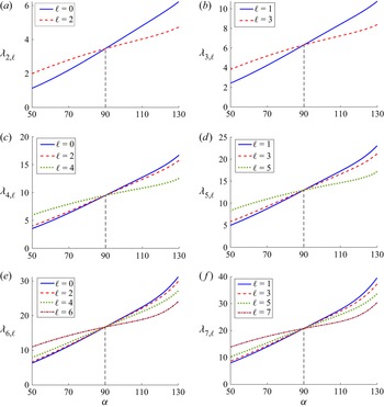
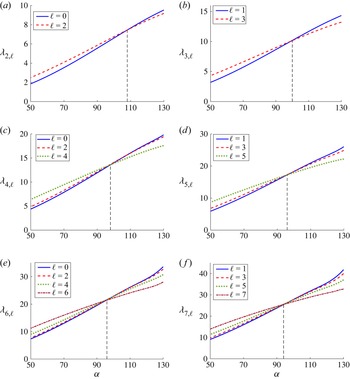
Figures 9 and 10 show how the azimuthal modes ( $\ell \neq 0,1$) break the hemispherical base state degeneracy for free and pinned disturbances, respectively. Recall that there is no effect of the equilibrium bubble pressure
 $\varPi$ whenever
 $\ell \neq 0$. The free modes with
 $\alpha =90^\circ$ are precisely theRayleigh–Lamb modes, since these sessile bubble modes can be extended smoothly to the full bubble by symmetry extension, i.e. reflection. Here, for fixed polar mode number
 $k$, frequencies split lower (higher) for super-hemispherical
 $\alpha <90^\circ$ (sub-hemispherical
 $\alpha > 90^\circ$) base states with increasing azimuthal mode number
 $\ell$ (cf. figure 9). The degeneracy centre shifts to higher
 $\alpha$ for pinned disturbances, as shown in figure 10. Each curve, irrespective of pinned or free disturbance, increases monotonically with increasing
 $\alpha$ because of the higher fluid inertia (volume) associated with sub-hemispherical
 $\alpha >90^\circ$ base states, which biases towards lower frequency. For fixed
 $k$, the slope of the curve increases with decreasing
 $\ell$, suggesting that the sectoral modes
 $k=\ell$ are less affected by base-state volume, because their motion is primarily horizontal. In contrast, modes with lower
 $\ell$, i.e. the zonal
 $\ell =0$ modes, have predominantly vertical motion and have a stronger effect with
 $\alpha$. Frequency splitting is more prevalent for the free disturbances, as they are less constrained.
Oscillation frequency  $\lambda$ for the free modes against contact angle
 $\alpha$, as it depends upon azimuthal mode number
 $\ell$, for polar mode number (a)
 $k=2$, (b)
 $k=3$, (c)
 $k=4$, (d)
 $k=5$, (e)
 $k=6$, and (f)
 $k=7$.

Oscillation frequency  $\lambda$ for the pinned modes against contact angle
 $\alpha$, as it depends upon azimuthal mode number
 $\ell$, for polar mode number (a)
 $k=2$, (b)
 $k=3$, (c)
 $k=4$, (d)
 $k=5$, (e)
 $k=6$, and (f)
 $k=7$.

4. Concluding remarks
We have analysed the hydrodynamic stability of a sessile bubble, showing how the frequency spectrum depends upon the wetting properties through the static contact angle  $\alpha$, equilibrium bubble pressure
 $\varPi$, and contact-line dynamics, for either pinned or freely moving (free) disturbances. Solutions have been computed by a Rayleigh–Ritz procedure and yield modes that can defined by the mode number pair
 $[k,\ell ]$ using an identification scheme inherited from the spherical harmonics
 $k+\ell =\mathbb {Z}^{+}_{even}$. Most motions are oscillatory. However, we do identify two instabilities: the
 $[0,0]$ breathing mode associated with volume change through gas compressibility, and the
 $[1,1]$ mode with instability mechanism analogous to the walking instability for the sessile drop (Bostwick & Steen Reference Bostwick and Steen2014). The instability mechanisms are described and stability diagrams mapped out in the parameter space. For a free bubble, volume-change and shape-change modes are decoupled typically, but for a sessile bubble, we show that these modes can interact in a complex manner. Finally, we show how the degeneracy of the Rayleigh–Lamb spectrum splits for the azimuthal
 $\ell \neq 0,1$ modes, and how this is related to the symmetry extensions of the sessile bubble modes.
The  $[0,0]$ breathing mode instability results in bubble collapse, and for the free disturbance this involves a dynamic receding motion of the contact line. Instability results because this motion decreases the potential energy of the system. Dynamic contact-line behaviour is often more complex, and often invokes constitutive laws relating the contact angle to the contact-line speed,
 $\alpha =g(u_{CL})$. One example is the Davis–Hocking model
 $\alpha = \varLambda u_{CL}$, where
 $\varLambda$ is the contact-line mobility parameter, with limiting cases as the free
 $\varLambda =0$ and pinned
 $\varLambda =\infty$ disturbances that we consider here (Davis Reference Davis1980; Hocking Reference Hocking1987). For finite
 $\varLambda$, it has been shown that contact-line dissipation occurs even for inviscid fluids (Bostwick & Steen Reference Bostwick and Steen2016). In this case, the energy budget would change, and this would modify the instability properties for the breathing mode.
Finally, we highlight the coupling between the volume-change and shape-change modes for sessile bubbles, and how this might facilitate preferred motions, as seen in acoustically enhanced heat transfer in pool boiling (Douglas et al. Reference Douglas, Boziuk, Smith and Glezer2012). Here, acoustic fields induce shape oscillations in sessile bubbles, which makes bubble detachment from the heated surface easier, thus improving heat transfer rates. Our linear model does not predict bubble detachment, but could be extended in this direction. Finally, we note that there have been numerous recent experimental observations of sessile drop oscillations (Sharp et al. Reference Sharp, Farmer and Kelly2011; Sharp Reference Sharp2012; Chang et al. Reference Chang, Bostwick, Steen and Daniel2013, Reference Chang, Bostwick, Daniel and Steen2015), but comparatively few observations of sessile bubble oscillations, and this should be pursued further to verify the theory proposed here, which is applicable for bubbles of size  $r$ smaller than the capillary length
 $\ell _c=\sqrt {\sigma /\rho g}$,
 $r<\ell _c$, with negligible viscous effects as defined by the Ohnesorge number
 $Oh\equiv \nu /\sqrt {\sigma R/\rho } \ll 1$.
Funding
J.B.B. acknowledges support from NSF grant CMMI-1935590.
Declaration of interests
The authors report no conflict of interest.