1. Introduction
The translation or diffusion of particles along membranes or interfaces is of interest because it is a model system for describing basic features of interfacial hydrodynamics (Singh & Joseph Reference Singh and Joseph2005; Stone Reference Stone2010; Masoud & Shelley Reference Masoud and Shelley2014), it is important in cellular signalling in biology and biophysics (Saffman & Delbrück Reference Saffman and Delbrück1975; Alberts et al. Reference Alberts, Johnson, Lewis, Morgan, Raff, Roberts and Walter2002) and it can be used to deduce the rheological properties of surface films (Ortega, Ritacco & Rubio Reference Ortega, Ritacco and Rubio2010; Squires & Mason Reference Squires and Mason2010; Fuller & Vermant Reference Fuller and Vermant2012; Mendoza et al. Reference Mendoza, Guzman, Martinez-Pedrero, Ritacco, Rubio, Ortega, Starov and Miller2014; Samaniuk & Vermant Reference Samaniuk and Vermant2014; Evans & Levine Reference Evans and Levine2015).
The theoretical investigation of such motions of membrane-trapped particles began with Saffman and Delbrück’s study of the Brownian motion of a thin circular disk at a flat viscous incompressible interface bounded on one or both sides by a viscous Newtonian fluid (Saffman Reference Saffman1976, see also Saffman & Delbrück Reference Saffman and Delbrück1975). Saffman and Delbrück’s original theory was further developed by Hughes, Pailthorpe & White (Reference Hughes, Pailthorpe and White1981) and has been extended in a number of directions including multiple particle interactions (Dodd et al. Reference Dodd, Hammer, Sangani and Koch1995), thin (Evans & Sackmann Reference Evans and Sackmann1988) and arbitrary depth (Stone & Ajdari Reference Stone and Ajdari1998) sublayers and deformable domains at the fluid–air interface (Stone & McConnell Reference Stone and McConnell1995). Also, the motion of a thin disk lying at a surfactant-coated interface in close proximity to a rigid boundary has been studied including the possibility of membrane compressibility (Barentin et al. Reference Barentin, Ybert, di Meglio and Joanny1999); subsequent experiments have been performed to deduce surface viscosities from measurements of the drag on the particle (Barentin et al. Reference Barentin, Muller, Ybert, Joanny and di Meglio2000). In addition, several studies have treated long slender rigid objects translating in the plane (Fischer Reference Fischer2004b ; Levine, Liverpool & MacKintosh Reference Levine, Liverpool and MacKintosh2004; Verwijlen et al. Reference Verwijlen, Moldenaers, Stone and Vermant2011; Fitzgibbon et al. Reference Fitzgibbon, Shaqfeh, Fuller and Walker2014). Finally, it is worth noting that experiments with circular disks rotating in a single-component phospholipid monolayer at the air–water interface have documented viscoelastic responses, which highlight the rheological complexities possible even in relatively simple interfacial materials (Choi et al. Reference Choi, Steltenkamp, Zasadzinski and Squires2011; Kim et al. Reference Kim, Choi, Zasadzinski and Squires2011).
The mathematical problem considered originally by Saffman and Delbrück was that of a flat, disk-shaped particle of radius
 $R$
that spans the thickness of a fluid layer (a monolayer or bilayer) at a liquid–air or liquid–liquid interface. The object is assumed to move at a constant velocity
 $\boldsymbol{U}=U\boldsymbol{e}$
and the force
 $\boldsymbol{F}=-F\boldsymbol{e}$
on the object is calculated. Here,
 $\boldsymbol{e}$
is the unit vector in the direction of motion and the ratio
 $F/U$
is the (scalar) particle resistivity, which is related to the measurable translational diffusivity
 $D$
by a Stokes–Einstein relation
 $D=k_{B}T/(F/U)$
, where
 $k_{B}$
is the Boltzmann constant and
 $T$
is the temperature. The resistance comes from both the sub- and surface phases and the dynamics is conveniently characterized in terms of the Boussinesq number
 $Bo={\it\mu}_{m}h/({\it\mu}R)$
, where
 ${\it\mu}$
is the fluid viscosity,
 ${\it\mu}_{m}$
is the viscosity of the membrane fluid and
 $h$
is the thickness of the surface layer. The commonly discussed surface viscosity is
 ${\it\mu}_{s}={\it\mu}_{m}h$
. Saffman and Delbrück were interested in small proteins so
 $Bo\gg 1$
. However, frequently membrane-trapped objects (e.g. phase separated domains or tracer particles) are large, in which case
 $Bo\ll 1$
(e.g. Fischer, Dhar & Heinig Reference Fischer, Dhar and Heinig2006; Sickert, Rondelez & Stone Reference Sickert, Rondelez and Stone2007; Lishchuk Reference Lishchuk2014).
It is natural to expect that this fluid dynamics problem is closely related to the low-Reynolds-number motion of an infinitely thin circular disk translating along a clean interface separating a liquid from an inviscid gas. The drag in this case is
 $F^{Clean}=(16/3){\it\mu}RU$
(Happel & Brenner Reference Happel and Brenner1983), which is half of the drag on a disk translating edgewise in an infinite bath of a Newtonian fluid. In fact, for a large membrane-trapped disk in an incompressible interface of negligible viscosity (
 $Bo\ll 1$
) the drag is in fact larger than
 $F^{Clean}$
by a factor of 3∕2, i.e.
 $F=8{\it\mu}RU$
.
To understand these differences in forces when the interface is clean versus when it is covered by a film, it is necessary to recognize that the surface film places a severe constraint on the form of the velocity field in the surrounding bulk fluid. Let us denote the surface velocity field as
 $\boldsymbol{u}^{(m)}$
and the gradient along the surface as
 $\boldsymbol{{\rm\nabla}}_{s}$
. Then, if the surface film is incompressible,
 $\boldsymbol{{\rm\nabla}}_{s}\boldsymbol{\cdot }\boldsymbol{u}^{(m)}=0$
. Since the surrounding flow with velocity
 $\boldsymbol{u}$
is also incompressible, then
 $\boldsymbol{{\rm\nabla}}\boldsymbol{\cdot }\boldsymbol{u}=0$
. However, as the surface is planar, then in the vicinity of the surface, the incompressibility condition for the bulk flow may be written
 $\boldsymbol{{\rm\nabla}}_{s}\boldsymbol{\cdot }\boldsymbol{u}^{(m)}+(\partial u_{z}/\partial z)=0$
, where
 $z$
is the direction normal to the surface. Consequently, near
 $z=0$
we see that
 $(\partial u_{z}/\partial z)=0$
and as
 $u_{z}=0$
at
 $z=0$
(the surface is not deforming out of the plane), then
 $u_{z}=0$
throughout the fluid. We thus conclude that the fluid below the surface is constrained to move in planes
 $z=\text{constant}$
and this constraint leads to larger dissipation (larger velocity gradients, higher drag) than would ordinarily be expected. By contrast, when a thin disk moves edgewise in an unbounded Newtonian fluid (or at a clean planar interface), the velocity field has both in-plane and out-of-plane components.
The basic question then arises: what if the surface motion is generated by an object that protrudes into the subphase? In this case, even with an incompressible surface film present, the protrusion causes the flow to be fully three-dimensional, which changes the relative contributions of the surface and subphase resistances. The case of a sphere translating at an interface that is both viscous and compressible has been examined theoretically by Danov et al. (Reference Danov, Aust, Durst and Lange1995), Danov, Dimova & Pouligny (Reference Danov, Dimova and Pouligny2000) and Dimova et al. (Reference Dimova, Danov, Pouligny and Ivanov2000). The relevant conditions for most surfactant and biological systems, however, concerns an incompressible but viscous interface, which has been studied numerically by Fischer et al. (Reference Fischer, Dhar and Heinig2006) and analytically by Lishchuk (Reference Lishchuk2014). These studies are focussed primarily on the limit of low surface viscosity (i.e.
 $Bo\ll 1$
).
Here, we consider oblate spheroidal and spherical particles that protrude into the subphase and semi-analytically quantify the variation of the force as the degree of protrusion changes. We shall see that the qualitative description given above is consistent with detailed calculations based on geometric perturbation expansions in terms of the particle protrusion, below denoted with
 ${\it\varepsilon}$
. Moreover, it appears that just considering one term of the expansions is in very good agreement with available results for a half-submerged sphere (
 ${\it\varepsilon}=1$
). The method of calculation, which perturbs about a known result for thin disks, is useful for other viscous flow problems as well (e.g. Dörr et al.
Reference Dörr, Hardt, Masoud and Stone2015).
2. Motion of a membrane-trapped particle partially submerged in the subphase
2.1. Problem statement
We consider the translation at velocity
 $\boldsymbol{U}$
of a partially submerged particle in a flat planar membrane (lower boundary at
 $z=0$
) of thickness
 $h$
bounded below by a viscous Newtonian fluid and bounded above by air, whose resistance is neglected (see figure 1). This configuration is common in laboratory experiments probing biological membranes and analogous surfactant films (e.g. Gambin et al.
Reference Gambin, Lopez-Esparza, Reffay, Sierecki, Gov, Genest, Hodges and Urbach2006; Sickert et al.
Reference Sickert, Rondelez and Stone2007; Ally & Amirfazli Reference Ally and Amirfazli2010; Maestro et al.
Reference Maestro, Bonales, Ritacco, Fischer, Rubio and Ortega2011; Verwijlen et al.
Reference Verwijlen, Moldenaers, Stone and Vermant2011; Wang et al.
Reference Wang, Yordanov, Paroor, Mukhopadhyay, Li, Butt and Koynov2011). For this general problem, we will now utilize
 $R$
as the radius of the three-phase contact line, which can be different than the radius of the particle. We assume that dissipation due to a moving contact line and the nature of the interactions between the particle and the molecules that make up the membrane preclude rotation of the particle. Also, we neglect bending of the membrane.
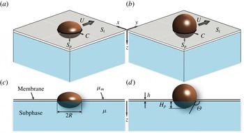
Particles straddling a liquid–air interface and protruding into the subphase. (a) A half-submerged oblate spheroid (i.e. contact angle is
 ${\it\Theta}=90^{\circ }$
). (b) A spherical particle making a contact angle of
 ${\it\Theta}>90^{\circ }$
.
 $S_{i}$
,
 $S_{p}$
, and
 $C$
denote, respectively, the membrane–subphase interface, surface area of the particle in contact with the subphase, and three-phase contact line. (c,d) Side views of (a,b).

The full problem we wish to consider includes the solution of Stokes equations in the subphase, and the solution of Stokes equations for an incompressible planar membrane fluid, supplemented by stress coupling with the subphase. The incompressibility assumption has been argued theoretically based on rapid equilibration due to Marangoni stresses (e.g. Fischer Reference Fischer2004a ) and has been supported experimentally (e.g. Barentin et al. Reference Barentin, Muller, Ybert, Joanny and di Meglio2000; Sickert et al. Reference Sickert, Rondelez and Stone2007). We note, however, that there are indications from macroscopic rheology and diffusion measurements that suggest possible effects of compressibility (e.g. Samaniuk & Vermant Reference Samaniuk and Vermant2014). In the work reported here, we assume an incompressible membrane flow.
It is convenient to work in cylindrical coordinates (
 $r,{\it\theta},z$
). We shall consistently denote membrane fields with a superscript
 $m$
(except for the viscosity of the membrane
 ${\it\mu}_{m}$
). Denoting the velocity, pressure and stress fields, respectively,
 $\boldsymbol{u}$
,
 $p$
, and
 ${\bf\sigma}$
, the equations for the two phases are
 $$\begin{eqnarray}\boldsymbol{{\rm\nabla}}\boldsymbol{\cdot }{\bf\sigma}=-\boldsymbol{{\rm\nabla}}p+{\it\mu}{\rm\nabla}^{2}\boldsymbol{u}=\mathbf{0},\quad \boldsymbol{{\rm\nabla}}\boldsymbol{\cdot }\boldsymbol{u}=0\quad (z<0),\end{eqnarray}$$
 $$\begin{eqnarray}\boldsymbol{{\rm\nabla}}_{s}\boldsymbol{\cdot }{\bf\sigma}^{(m)}+h^{-1}\boldsymbol{n}\boldsymbol{\cdot }{\bf\sigma}=-\boldsymbol{{\rm\nabla}}_{s}\,p^{(m)}+{\it\mu}_{m}{\rm\nabla}_{s}^{2}\boldsymbol{u}^{(m)}+h^{-1}\boldsymbol{n}\boldsymbol{\cdot }{\bf\sigma}=\mathbf{0},\end{eqnarray}$$
 $$\begin{eqnarray}\boldsymbol{{\rm\nabla}}_{s}\boldsymbol{\cdot }\boldsymbol{u}^{(m)}=0\quad \text{at }z=0\;(r>R),\end{eqnarray}$$
 $$\begin{eqnarray}\boldsymbol{u}=\boldsymbol{U}\quad \text{on }S_{p}~(0\leqslant r\leqslant R\text{ and }z\neq 0\text{ in general}),\end{eqnarray}$$
 $$\begin{eqnarray}\boldsymbol{u}(r,{\it\theta},0)=\boldsymbol{u}^{(m)}(r,{\it\theta})\quad \text{at }z=0\;(r>R),\end{eqnarray}$$
where
 $\boldsymbol{n}$
is the unit normal from the surface film and directed into the subphase
 $(\boldsymbol{n}=\boldsymbol{e}_{z})$
,
 $R$
is the radius of the three-phase contact line
 $C$
,
 $S_{p}$
is the surface area of the particle in contact with the subphase, and
 $\boldsymbol{{\rm\nabla}}_{s}$
denotes the derivative operator in the plane of the interface. Here, the membrane fluid is treated as satisfying three-dimensional equations, but motion occurs only parallel to the plane
 $z=0$
and without transverse shear. The term
 $h^{-1}\boldsymbol{n}\boldsymbol{\cdot }{\bf\sigma}$
in (2.1c
) corresponds to the force per unit volume exerted on the surface fluid from the stresses due to motion in the subphase. The oft-mentioned surface pressure (or interfacial tension)
 ${\rm\pi}_{s}$
corresponds to
 ${\rm\pi}_{s}=p^{(m)}h$
and the surface viscosity is
 ${\it\mu}_{s}={\it\mu}_{m}h$
, though we shall not use these designations here.
To be specific, we consider two particle shapes: a half-submerged oblate spheroid (i.e. contact angle is
 ${\it\Theta}=90^{\circ }$
); and a partially submerged sphere making a contact angle of
 ${\it\Theta}\geqslant 90^{\circ }$
(figure 1). The wetted surfaces of the spheroidal and spherical particles are described, respectively, by
 $$\begin{eqnarray}z=R{\it\varepsilon}\sqrt{1-\left(\frac{r}{R}\right)^{2}}\end{eqnarray}$$
and
 $$\begin{eqnarray}z=\frac{R{\it\varepsilon}}{1+\cos {\it\Theta}}\left[\sqrt{1-\left(\frac{r}{R}\right)^{2}\sin ^{2}{\it\Theta}}+\cos {\it\Theta}\right],\end{eqnarray}$$
where
 ${\it\varepsilon}=H_{p}/R$
is the ratio of the maximum protrusion length
 $H_{p}$
and the radius of the three-phase contact line
 $R$
(see figure 1), and
 ${\it\Theta}=2\,\arctan (1/{\it\varepsilon})$
in (2.2b
). If we set
 ${\it\varepsilon}=0$
, we recover a flat circular disk translating along the membrane–subphase interface, first analysed by Saffman (Reference Saffman1976). Here, we assume
 ${\it\varepsilon}\ll 1$
. Then, to the leading order in
 ${\it\varepsilon}$
, (2.2) can be written succinctly as
 $$\begin{eqnarray}z=R[{\it\varepsilon}f(r)+O({\it\varepsilon}^{2})],\end{eqnarray}$$
where the shape function
 $f(r)=\sqrt{1-(r/R)^{2}}$
and
 $f(r)=1-(r/R)^{2}$
for the spheroids and spheres, respectively. Note that
 $O({\it\varepsilon}^{2})$
term vanishes for the spheroids (see (2.2a
)). As a result, the shape of partially submerged spheres with
 ${\it\varepsilon}\approx 1$
is better approximated by (2.3) when the shape function of spheroids is used.
For the detailed calculation, it is convenient to utilize the Lorentz reciprocal theorem from low-Reynolds-number hydrodynamics (e.g. Happel & Brenner Reference Happel and Brenner1983). As will be shown, it is possible to determine the change in the force on the particle at
 $O({\it\varepsilon})$
, accounting for the influence of both the monolayer and subphase flows, without determining the detailed velocity and pressure distributions at
 $O({\it\varepsilon})$
. The reciprocal theorem has been previously employed to facilitate the calculation of desired integral quantities in Stokes flow problems by eliminating the need for developing detailed flow fields (e.g. Leal Reference Leal1980; Haj-Hariri, Nadim & Borhan Reference Haj-Hariri, Nadim and Borhan1993; Stone & Samuel Reference Stone and Samuel1996; Masoud & Stone Reference Masoud and Stone2014; Dörr et al.
Reference Dörr, Hardt, Masoud and Stone2015). We non-dimensionalize the equations and boundary conditions using the radius of the three-phase contact line
 $R$
as the characteristic length scale, the translational speed
 $U$
as the velocity scale and the scale
 ${\it\mu}U/R$
as the characteristic pressure or stress. Then, all material and geometric parameters disappear except for the dimensionless parameter
 $Bo^{-1}={\it\mu}R/({\it\mu}_{m}h)$
that appears in the equation for the surface flow (replacing
 $h^{-1}$
in (2.1c
)). The full problem is now completely specified in terms of two-dimensionless parameters
 $Bo$
and
 ${\it\varepsilon}$
.
2.2. Solution via a perturbation expansion
Since we are interested in a protrusion into the subphase, we introduce a (regular) perturbation expansion for the velocity and hydrodynamic force on the particle in the forms
 $$\begin{eqnarray}\displaystyle & \boldsymbol{u}=\boldsymbol{u}^{(0)}+{\it\varepsilon}\boldsymbol{u}^{(1)}+O({\it\varepsilon}^{2}), & \displaystyle\end{eqnarray}$$
 $$\begin{eqnarray}\displaystyle & \boldsymbol{F}=\boldsymbol{F}^{(0)}+{\it\varepsilon}\boldsymbol{F}^{(1)}+O({\it\varepsilon}^{2}). & \displaystyle\end{eqnarray}$$
 $z={\it\varepsilon}f(r)$
, in terms of a Taylor series about
 $z=0$
. Then, the velocity at
 $z=0$
is given by
 $\boldsymbol{u}=\boldsymbol{u}^{(0)}+{\it\varepsilon}[\boldsymbol{u}^{(1)}+f(r)(\partial \boldsymbol{u}^{(0)}/\partial z)]+O({\it\varepsilon}^{2})$
. All boundary conditions from now on are applied at
 $z=0$
with
 $r\leqslant 1$
or
 $r>1$
.
At
 $O(1)$
we must solve the so-called Saffman–Delbrück problem,
 $$\begin{eqnarray}\boldsymbol{{\rm\nabla}}\boldsymbol{\cdot }{\bf\sigma}^{(0)}=-\boldsymbol{{\rm\nabla}}p^{(0)}+{\rm\nabla}^{2}\boldsymbol{u}^{(0)}=\mathbf{0},\quad \boldsymbol{{\rm\nabla}}\boldsymbol{\cdot }\boldsymbol{u}^{(0)}=0,\end{eqnarray}$$
 $$\begin{eqnarray}\boldsymbol{u}^{(0)}=\boldsymbol{U}\quad \text{at }z=0\;(r\leqslant 1),\end{eqnarray}$$
 $$\begin{eqnarray}\boldsymbol{{\rm\nabla}}_{s}\boldsymbol{\cdot }{\bf\sigma}^{(m0)}+Bo^{-1}\boldsymbol{n}\boldsymbol{\cdot }{\bf\sigma}^{(0)}=\mathbf{0},\quad \boldsymbol{{\rm\nabla}}_{s}\boldsymbol{\cdot }\boldsymbol{u}^{(m0)}=0\quad \text{at }z=0\;(r>1).\end{eqnarray}$$
The hydrodynamic force
 $\boldsymbol{F}^{(0)}$
as a function of
 $Bo$
is known (Hughes et al.
Reference Hughes, Pailthorpe and White1981; Stone & Ajdari Reference Stone and Ajdari1998). In particular, for
 $Bo\ll 1$
,
 $\boldsymbol{F}^{(0)}=-8{\it\mu}R\boldsymbol{U}$
, which is a factor of
 $3/2$
larger than for a flat disk translating edgewise at a perfectly clean interface (e.g. see appendix A of Stone & Ajdari Reference Stone and Ajdari1998). The physical reason for this enhanced drag was discussed in the introduction.
At
 $O({\it\varepsilon})$
, we consider
 $$\begin{eqnarray}\boldsymbol{{\rm\nabla}}\boldsymbol{\cdot }{\bf\sigma}^{(1)}=-\boldsymbol{{\rm\nabla}}p^{(1)}+{\rm\nabla}^{2}\boldsymbol{u}^{(1)}=\mathbf{0},\quad \boldsymbol{{\rm\nabla}}\boldsymbol{\cdot }\boldsymbol{u}^{(1)}=0,\end{eqnarray}$$
 $$\begin{eqnarray}\boldsymbol{u}^{(1)}=-f(r)\frac{\partial \boldsymbol{u}^{(0)}}{\partial z}\quad \text{at }z=0\;(r\leqslant 1),\end{eqnarray}$$
 $$\begin{eqnarray}\boldsymbol{{\rm\nabla}}_{s}\boldsymbol{\cdot }{\bf\sigma}^{(m1)}+Bo^{-1}\boldsymbol{n}\boldsymbol{\cdot }{\bf\sigma}^{(1)}=\mathbf{0},\quad \boldsymbol{{\rm\nabla}}_{s}\boldsymbol{\cdot }\boldsymbol{u}^{(m1)}=0\quad \text{at }z=0\;(r>1).\end{eqnarray}$$
It is important that for the
 $O(1)$
and
 $O({\it\varepsilon})$
problems, (2.5) and (2.6), all boundary conditions are given at
 $z=0$
, unlike the original problem statement (see (2.1)).
2.3. Application of the reciprocal theorem
We now determine
 $\boldsymbol{F}^{(1)}$
, the hydrodynamic force on the particle associated with the protrusion in the third dimension. To this end, we introduce the reciprocal theorem as it is applied to this problem and refer to figure 1 for the necessary notation (the use of the reciprocal theorem to study the simpler Stokes flow problem of a translating thin oblate spheroid is outlined in the appendix A). This approach takes advantage of the fact that the solution to the leading-order problem
 $\boldsymbol{u}^{(0)}$
is known, in general numerically, by solving (2.5). As both the
 $O(1)$
and
 $O({\it\varepsilon})$
problems are now defined on the same domain, we begin with (e.g. Happel & Brenner Reference Happel and Brenner1983, p. 85)
 $$\begin{eqnarray}\int _{S_{d}+S_{i}}\boldsymbol{n}\boldsymbol{\cdot }{\bf\sigma}^{(1)}\boldsymbol{\cdot }\boldsymbol{u}^{(0)}\,\text{d}S=\int _{S_{d}+S_{i}}\boldsymbol{n}\boldsymbol{\cdot }{\bf\sigma}^{(0)}\boldsymbol{\cdot }\boldsymbol{u}^{(1)}\,\text{d}S,\end{eqnarray}$$
where
 $S_{d}$
and
 $S_{i}$
denote, respectively, the surface of the disk (
 $z=0$
) and membrane–subphase interface. Integrals over a large bounding surface
 $S_{\infty }$
are zero since velocities decay at least as fast as the inverse distance in the far field.
Several substitutions are now possible. On the surface of the disk, we have
 $\boldsymbol{u}^{(0)}=\boldsymbol{U}$
, which is a constant vector, and also
 $\boldsymbol{u}^{(1)}=-f(r)(\partial \boldsymbol{u}^{(0)}/\partial z)$
. Along the membrane–subphase interface, we have
 $\boldsymbol{n}\boldsymbol{\cdot }{\bf\sigma}^{(i)}=-Bo\boldsymbol{{\rm\nabla}}_{s}\boldsymbol{\cdot }{\bf\sigma}^{(mi)}$
for
 $i=0,1$
. Thus we see that
 $$\begin{eqnarray}\displaystyle \boldsymbol{F}_{sub}^{(1)}\boldsymbol{\cdot }\boldsymbol{U} & = & \displaystyle -\int _{S_{d}}f(r)\left(\frac{\partial \boldsymbol{u}^{(0)}}{\partial z}\right)^{2}\,\text{d}S-Bo\int _{S_{i}}(\boldsymbol{{\rm\nabla}}_{s}\boldsymbol{\cdot }{\bf\sigma}^{(m0)})\boldsymbol{\cdot }\boldsymbol{u}^{(1)}\,\text{d}S\nonumber\\ \displaystyle & & \displaystyle +\,Bo\int _{S_{i}}(\boldsymbol{{\rm\nabla}}_{s}\boldsymbol{\cdot }{\bf\sigma}^{(m1)})\boldsymbol{\cdot }\boldsymbol{u}^{(0)}\,\text{d}S,\end{eqnarray}$$
where
 $\boldsymbol{F}_{sub}^{(1)}=\int _{S_{d}}\boldsymbol{n}\boldsymbol{\cdot }{\bf\sigma}^{(1)}\,\text{d}S$
is the
 $O({\it\varepsilon})$
contribution to the force from the subphase alone. In arriving at the form of the first term on the right-hand side of (2.8), we have utilized the fact that the flow
 $\boldsymbol{u}^{(0)}$
has no
 $z$
-component.
To evaluate the second and third integrals on the right-hand side of (2.8), we first note that
 $\boldsymbol{{\rm\nabla}}_{s}\boldsymbol{\cdot }({\bf\sigma}\boldsymbol{\cdot }\boldsymbol{u})=(\boldsymbol{{\rm\nabla}}_{s}\boldsymbol{\cdot }{\bf\sigma})\boldsymbol{\cdot }\boldsymbol{u}+{\bf\sigma}\boldsymbol{ : }\boldsymbol{{\rm\nabla}}_{s}\boldsymbol{u}$
. Then, we use the divergence theorem to convert the integrals over the interface
 $S_{i}$
into integrals over the contours
 $C$
and
 $C_{\infty }$
that, respectively, bound the inside and outside of the membrane–subphase interface (see figure 1). Integrals over
 $C_{\infty }$
may be shown to vanish. Hence, we find
 $$\begin{eqnarray}\displaystyle & \displaystyle \int _{S_{i}}(\boldsymbol{{\rm\nabla}}_{s}\boldsymbol{\cdot }{\bf\sigma}^{(m0)})\boldsymbol{\cdot }\boldsymbol{u}^{(1)}\,\text{d}S=\int _{C}\boldsymbol{n}\boldsymbol{\cdot }{\bf\sigma}^{(m0)}\boldsymbol{\cdot }\boldsymbol{u}^{(1)}\,\text{d}S-\int _{S_{i}}{\bf\sigma}^{(m0)}\boldsymbol{ : }\boldsymbol{{\rm\nabla}}_{s}\boldsymbol{u}^{(1)}\,\text{d}S, & \displaystyle\end{eqnarray}$$
 $$\begin{eqnarray}\displaystyle & \displaystyle \int _{S_{i}}(\boldsymbol{{\rm\nabla}}_{s}\boldsymbol{\cdot }{\bf\sigma}^{(m1)})\boldsymbol{\cdot }\boldsymbol{u}^{(0)}\,\text{d}S=\int _{C}\boldsymbol{n}\boldsymbol{\cdot }{\bf\sigma}^{(m1)}\boldsymbol{\cdot }\boldsymbol{u}^{(0)}\,\text{d}S-\int _{S_{i}}{\bf\sigma}^{(m1)}\boldsymbol{ : }\boldsymbol{{\rm\nabla}}_{s}\boldsymbol{u}^{(0)}\,\text{d}S. & \displaystyle\end{eqnarray}$$
 $\boldsymbol{u}^{(1)}=\mathbf{0}$
as the particle surface is approached (see (2.6c
)). Also,
 $\boldsymbol{u}^{(0)}=\boldsymbol{U}$
on
 $C$
and, therefore, can be taken out of the first integral on the right-hand side of (2.9b
). Lastly, the integrals over
 $S_{i}$
on the right-hand sides of (2.9a
) and (2.9b
) are equal as the surface velocity fields
 $\boldsymbol{u}^{(mi)}$
are incompressible, leading to
 ${\bf\sigma}^{(m)}=-p^{(m)}(\unicode[STIX]{x1D644}-\boldsymbol{e}_{z}\boldsymbol{e}_{z})+2{\it\mu}_{m}\unicode[STIX]{x1D640}^{(m)}$
. Here,
 $\unicode[STIX]{x1D644}$
is the unit tensor and
 $\unicode[STIX]{x1D640}^{(m)}=[\boldsymbol{{\rm\nabla}}_{s}\boldsymbol{u}^{(m)}+(\boldsymbol{{\rm\nabla}}_{s}\boldsymbol{u}^{(m)})]/2$
is the surface rate-of-strain tensor (see Happel & Brenner Reference Happel and Brenner1983, p. 86, for an analogous idea). Thus, the substitution of (2.9) in (2.8) yields
 $$\begin{eqnarray}\boldsymbol{F}^{(1)}\boldsymbol{\cdot }\boldsymbol{U}\equiv \boldsymbol{F}_{sub}^{(1)}\boldsymbol{\cdot }\boldsymbol{U}-Bo\int _{C}\boldsymbol{n}\boldsymbol{\cdot }{\bf\sigma}^{(m1)}\,\text{d}S\boldsymbol{\cdot }\boldsymbol{U}=-\int _{S_{d}}f(r)\left(\frac{\partial \boldsymbol{u}^{(0)}}{\partial z}\right)^{2}\,\text{d}S,\end{eqnarray}$$
where again we use the convention that
 $\boldsymbol{n}$
is outward from
 $S_{i}$
. In (2.10), the integral over the contour
 $C$
gives the membrane contribution to the force on the particle. The sum of the two force terms thus provides, at
 $O({\it\varepsilon})$
, the total hydrodynamic force
 $\boldsymbol{F}^{(1)}$
exerted on the object.
The integral on the right-hand side of (2.10) can be evaluated numerically as a function of
 $Bo$
since
 $\boldsymbol{u}^{(0)}$
is the known Saffman–Delbrück solution. Equation (2.10) is the principal result of this section and allows evaluation of the influence of the protrusion and shape (through the function
 $f(r)$
) on the correction to the force on the membrane-trapped particle.
3. Numerical evaluation of the
 $O({\it\varepsilon})$
contribution to the force

In order to evaluate the integral expression (2.10), and so the force (2.4b
) on the particle, we must solve the Saffman–Delbrück problem. Here, we make use of the solution form presented by Stone & Ajdari (Reference Stone and Ajdari1998), specialized for the case of an infinite depth subphase (
 $H/R\rightarrow \infty$
in their notation, where
 $H$
is the depth of the subphase; the Matlab code developed for numerical calculations is available upon request). The velocity field in the subphase only has
 $r$
and
 ${\it\theta}$
components given by
 $$\begin{eqnarray}\displaystyle & \displaystyle u_{r}^{(0)}(r,{\it\theta},z)=\cos {\it\theta}\int _{0}^{\infty }A(s)\text{e}^{-sz}[\text{J}_{2}(sr)+\text{J}_{0}(sr)]\,\text{d}s, & \displaystyle\end{eqnarray}$$
 $$\begin{eqnarray}\displaystyle & \displaystyle u_{{\it\theta}}^{(0)}(r,{\it\theta},z)=\sin {\it\theta}\int _{0}^{\infty }A(s)\text{e}^{-sz}[\text{J}_{2}(sr)-\text{J}_{0}(sr)]\,\text{d}s, & \displaystyle\end{eqnarray}$$
 $\text{J}_{m}$
are Bessel functions of the first kind. The function
 $A(s)$
is evaluated in the form
 $$\begin{eqnarray}A(s)=\frac{s^{-1-{\it\beta}}}{s+Bo^{-1}}\mathop{\sum }_{m=0}^{\infty }a_{m}\text{J}_{2m+1+{\it\beta}}(s),\end{eqnarray}$$
where
 ${\it\beta}$
may be chosen to assist evaluation of the integrals below. The coefficients
 $\{a_{m}\}$
are obtained from the linear system of equations
 $$\begin{eqnarray}\mathop{\sum }_{m=0}^{\infty }a_{m}\int _{0}^{\infty }\frac{s^{-2-2{\it\beta}}}{s+Bo^{-1}}\text{J}_{2m+1+{\it\beta}}(s)\text{J}_{2n+1+{\it\beta}}(s)\,\text{d}s=\frac{{\it\delta}_{0n}}{2^{{\it\beta}+1}{\it\Gamma}({\it\beta}+2)},\quad n=0,1,2,\ldots ,\end{eqnarray}$$
where
 ${\it\delta}_{ij}$
is the Kronecker delta function. For the results reported below we chose
 ${\it\beta}=-1/2$
and typically kept ten coefficients in the evaluation of the linear system. Note that the dimensional force in the Saffman–Delbrück problem, the
 $O(1)$
problem from the previous section, is (Stone & Ajdari Reference Stone and Ajdari1998)
 $$\begin{eqnarray}\boldsymbol{F}^{(0)}=-4\sqrt{2{\rm\pi}}Bo{\it\mu}R\boldsymbol{U}a_{0},\end{eqnarray}$$
where
 $a_{0}$
is a function of
 $Bo$
.
With the
 $\{a_{m}\}$
known, we evaluate the velocity derivatives according to
 $$\begin{eqnarray}\displaystyle & \displaystyle \left.\frac{\partial u_{r}^{(0)}}{\partial z}\right|_{z=0}=-\!\cos {\it\theta}\int _{0}^{\infty }A(s)s\,[\text{J}_{2}(sr)+\text{J}_{0}(sr)]\,\text{d}s, & \displaystyle\end{eqnarray}$$
 $$\begin{eqnarray}\displaystyle & \displaystyle \left.\frac{\partial u_{{\it\theta}}^{(0)}}{\partial z}\right|_{z=0}=-\!\sin {\it\theta}\int _{0}^{\infty }A(s)s\,[\text{J}_{2}(sr)-\text{J}_{0}(sr)]\,\text{d}s. & \displaystyle\end{eqnarray}$$
 $\boldsymbol{F}^{(1)}$
and
 $\boldsymbol{U}$
are collinear, we evaluate numerically the integral
 $$\begin{eqnarray}F^{(1)}=\int _{0}^{2{\rm\pi}}\int _{0}^{1}f(r)\left[\left(\left.\frac{\partial u_{r}^{(0)}}{\partial z}\right|_{z=0}\right)^{2}+\left(\left.\frac{\partial u_{{\it\theta}}^{(0)}}{\partial z}\right|_{z=0}\right)^{2}\right]\,r\,\text{d}r\,\text{d}{\it\theta}.\end{eqnarray}$$
The
 ${\it\theta}$
integration is simple, and the
 $r$
integration is performed numerically by even discretization of the interval
 $0\leqslant r\leqslant 1$
. Thus, we arrive at a numerical evaluation of the influence of shape (
 $f(r)$
), the degree of protrusion (
 ${\it\varepsilon}$
) and the viscosity contrast (
 $Bo$
) on the force on a membrane-trapped particle that protrudes into the subphase. As mentioned earlier, the shapes considered here are half-submerged oblate spheroids with
 ${\it\Theta}=90^{\circ }$
and partially submerged spheres with
 ${\it\Theta}\geqslant 90^{\circ }$
(see figure 1 and (2.2)–(2.3)).
4. Discussion
We present the results for the relative influence of the finite thickness by plotting
 $F^{(1)}/F^{(0)}$
versus
 $Bo$
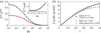
for a half-submerged oblate spheroid and a partially submerged sphere (see figure 2
a). For completeness, we also plot
 $F^{(0)}$
in the dimensionless form as a function of
 $Bo$
(see the inset). Analytical estimates of
 $F^{(0)}$
in the limits of
 $Bo\ll 1$
and
 $Bo\gg 1$
are given in Stone & Ajdari (Reference Stone and Ajdari1998). We believe that these results are the first to account for the particle protrusion into the subphase for the practically relevant case of an incompressible surface film and for the whole range of
 $Bo$
.
(a) The ratio of
 $O({\it\varepsilon})$
and
 $O(1)$
contributions to the drag on the particle as a function of the Boussinesq number
 $Bo$
. The circles and diamonds represent the results for half-submerged oblate spheroids with
 ${\it\Theta}=90^{\circ }$
and partially submerged spheres with
 ${\it\Theta}\geqslant 90^{\circ }$
, respectively. The inset in (a) shows the variation of
 $F^{(0)}$
, the hydrodynamic force in the Saffman–Delbrück problem, versus
 $Bo$
. (b) Dimensionless force on the particle versus the dimensionless protrusion length
 ${\it\varepsilon}$
for
 $Bo\ll 1$
.

To characterize the effect of the protrusion, we compare the total force
 $F=F^{(0)}+{\it\varepsilon}F^{(1)}+O({\it\varepsilon}^{2})$
to the case of the same object translating at a clean interface. We denote the force in the latter
 $F^{Clean}$
, which is a well-known function of the aspect ratio
 ${\it\varepsilon}$
. As given in the appendix A, for
 ${\it\varepsilon}\ll 1$
(and only taking the force on half of the particle),
 $F^{Clean}=(16/3)[1+(4{\it\alpha}/3{\rm\pi}){\it\varepsilon}+O({\it\varepsilon}^{2})]$
. Here,
 ${\it\alpha}=(1,2)$
for partially submerged spheres and half-submerged spheroids, respectively (see (A 9) and (A 10)). Consequently, we consider
 $$\begin{eqnarray}\frac{F}{F^{Clean}}=\frac{F^{(0)}+{\it\varepsilon}F^{(1)}+O({\it\varepsilon}^{2})}{\displaystyle \frac{16}{3}\left[1+\frac{4{\it\alpha}}{3{\rm\pi}}{\it\varepsilon}+O({\it\varepsilon}^{2})\right]}=\frac{3F^{(0)}}{16}\left[1+{\it\varepsilon}\left(\frac{F^{(1)}}{F^{(0)}}-\frac{4{\it\alpha}}{3{\rm\pi}}\right)+O({\it\varepsilon}^{2})\right].\end{eqnarray}$$
Figure 2(a) shows that the term
 $F^{(1)}/F^{(0)}-4{\it\alpha}/3{\rm\pi}$
in (4.1) is negative for all values of
 $Bo$
, which implies that the protrusion lessens the effect of the incompressible surface film and that the subphase contributes progressively more to the drag. This trend is consistent with the results of Danov et al. (Reference Danov, Aust, Durst and Lange1995), who considered the case of a sphere translating along a flat, compressible and surfactant-coated interface.
Finally, we compare our results for the particle drag with the numerical calculations of Fischer et al. (Reference Fischer, Dhar and Heinig2006) for a partially submerged sphere trapped in an incompressible membrane of zero viscosity (see figure 2
b). We see that for
 ${\it\varepsilon}\leqslant 0.6$
their data (solid line in figure 2
b) is very well represented by our perturbation expansion results for partially submerged spheres (diamonds) while the results for half-submerged oblate spheroids (circles) provide a better match for
 $0.6<{\it\varepsilon}\leqslant 1$
. Overall, our calculations indicate that only considering the first-order term in the perturbation expansion in
 ${\it\varepsilon}$
provides very good estimates for the drag on membrane-trapped particles with a dimensionless protrusion length up to
 ${\it\varepsilon}=1$
.
Acknowledgements
H.A.S. thanks F. Rondelez and M. Sickert for bringing this problem to his attention in the early 2000s and A. Ajdari, T. Fischer, F. Rondelez, and M. Sickert for valuable discussions. D. Lubensky is thanked for conversations that took place many years ago. ESPCI, the Laboratoire PCT, and the City of Paris are thanked for their support during a visit in 2001 when this work was partially completed. H.M. acknowledges support from DOE grant DE-FG02-88ER25053 and from NSF grant DMR-0844115 and the Institute for Complex Adaptive Matter.
Appendix A. Edgewise translation of a thin oblate spheroid
The low-Reynolds-number edgewise translation at speed
 $U$
of an oblate spheroid in a Newtonian fluid is described in detail in Happel & Brenner (Reference Happel and Brenner1983) and an analytical result is available. The dimensional force depends on the aspect ratio
 ${\it\varepsilon}$
and is given by
 $$\begin{eqnarray}\frac{F^{Stokes}}{6{\rm\pi}{\it\mu}UR}=\frac{8}{3}\left[\frac{3-2{\it\varepsilon}^{2}}{(1-{\it\varepsilon}^{2})^{3/2}}\sin ^{-1}\left(\sqrt{1-{\it\varepsilon}^{2}}\right)-\frac{{\it\varepsilon}}{1-{\it\varepsilon}^{2}}\right]^{-1},\end{eqnarray}$$
which for
 ${\it\varepsilon}\ll 1$
yields
 $$\begin{eqnarray}\frac{F^{Stokes}}{6{\rm\pi}{\it\mu}UR}=\frac{16}{9{\rm\pi}}\left[1+\frac{8{\it\varepsilon}}{3{\rm\pi}}+O({\it\varepsilon}^{2})\right].\end{eqnarray}$$
Rather surprisingly, the
 $O({\it\varepsilon})$
correction to the drag is actually valid to within 5 % for all
 $0\leqslant {\it\varepsilon}\leqslant 1$
(simply plot the two functions). To make this point clear, the estimate for the force on a sphere is obtained by setting
 ${\it\varepsilon}=1$
. Of course, equation (A 1) yields
 $F^{Stokes}=6{\rm\pi}{\it\mu}UR$
while (A 2) yields the estimate
 $F^{Stokes}=6{\rm\pi}{\it\mu}UR\times 1.046\ldots .$
It is useful to illustrate how the reciprocal theorem may be applied to obtain the
 $O({\it\varepsilon})$
correction, (A 2). We wish to solve the Stokes equations and scale all lengths by the radius
 $R$
, velocities by the speed
 $U$
and pressure and stresses by
 ${\it\mu}U/R$
. Hence, we consider
 $$\begin{eqnarray}\boldsymbol{{\rm\nabla}}\boldsymbol{\cdot }{\bf\sigma}=-\boldsymbol{{\rm\nabla}}p+{\rm\nabla}^{2}\boldsymbol{u}=\mathbf{0},\quad \boldsymbol{{\rm\nabla}}\boldsymbol{\cdot }\boldsymbol{u}=0,\end{eqnarray}$$
 $$\begin{eqnarray}\boldsymbol{u}=\boldsymbol{U}\quad \text{on }S_{p}.\end{eqnarray}$$
As above, we denote the surface of the spheroid in (dimensionless) cylindrical
 $(r,{\it\theta},z)$
coordinates by
 $z={\it\varepsilon}f(r)=\pm {\it\varepsilon}\sqrt{1-r^{2}}$
.
It is natural to seek the solution of a perturbation expansion in
 ${\it\varepsilon}$
, i.e.
 $\boldsymbol{u}=\boldsymbol{u}^{(0)}+{\it\varepsilon}\boldsymbol{u}^{(1)}+O({\it\varepsilon}^{2})$
. Similar to § 2.1, we use a Taylor series of the velocity about the flat (circular disk) shape, so that at
 $z=0$
the velocity is given by
 $\boldsymbol{u}=\boldsymbol{u}^{(0)}+{\it\varepsilon}[\boldsymbol{u}^{(1)}+f(r)(\partial \boldsymbol{u}^{(0)}/\partial z)]+O({\it\varepsilon}^{2})$
.
At the leading-order, we have the known solution for the velocity and pressure fields of a circular disk translating edgewise, e.g.
 $F^{(0)}=32/3$
in dimensionless terms. At
 $O({\it\varepsilon})$
, we seek to solve
 $$\begin{eqnarray}\boldsymbol{{\rm\nabla}}\boldsymbol{\cdot }{\bf\sigma}^{(1)}=\boldsymbol{{\rm\nabla}}p^{(1)}+{\rm\nabla}^{2}\boldsymbol{u}^{(1)}=\mathbf{0},\quad \boldsymbol{{\rm\nabla}}\boldsymbol{\cdot }\boldsymbol{u}^{(1)}=0,\end{eqnarray}$$
 $$\begin{eqnarray}\boldsymbol{u}^{(1)}=-f(r)\frac{\partial \boldsymbol{u}^{(0)}}{\partial z}\quad \text{at }z=0\;(r\leqslant 1).\end{eqnarray}$$
In order to obtain the force accompanying this motion, we use the reciprocal theorem, which results in (see (2.7) above)
 $$\begin{eqnarray}\int _{S_{d}}\boldsymbol{n}\boldsymbol{\cdot }{\bf\sigma}^{(1)}\boldsymbol{\cdot }\boldsymbol{u}^{(0)}\,\text{d}S=\int _{S_{d}}\boldsymbol{n}\boldsymbol{\cdot }{\bf\sigma}^{(0)}\boldsymbol{\cdot }\boldsymbol{u}^{(1)}\,\text{d}S.\end{eqnarray}$$
Since
 $\boldsymbol{u}^{(0)}=\boldsymbol{U}$
on the surface and the integral of the stress is the
 $O({\it\varepsilon})$
force, we see that the left-hand side integral yields an expression involving the force
 $\boldsymbol{F}^{(1)}$
. The right-hand side also can be simplified since
 $\boldsymbol{n}=\pm \boldsymbol{e}_{z}$
. Hence, we have
 $$\begin{eqnarray}\boldsymbol{F}^{(1)}\boldsymbol{\cdot }\boldsymbol{U}=-\int _{S_{d}}f(r)(\boldsymbol{e}_{z}\boldsymbol{\cdot }{\bf\sigma}^{(0)})\boldsymbol{\cdot }\frac{\partial \boldsymbol{u}^{(0)}}{\partial z}\,\text{d}S,\end{eqnarray}$$
which can be further reduced to (accounting for both sides of the disk)
 $$\begin{eqnarray}\boldsymbol{F}^{(1)}\boldsymbol{\cdot }\boldsymbol{U}=-2\int _{r=0}^{1}\int _{{\it\theta}=0}^{2{\rm\pi}}f(r)\left(\frac{\partial \boldsymbol{u}^{(0)}}{\partial z}\right)^{2}~r\,\text{d}r\,\text{d}{\it\theta}.\end{eqnarray}$$
The velocity field
 $\boldsymbol{u}^{(0)}$
for flow about a circular disk translating edgewise is known analytically (e.g. Davis Reference Davis1990; Tanzosh & Stone Reference Tanzosh and Stone1996),
 $$\begin{eqnarray}\displaystyle & \displaystyle u_{r}^{(0)}(r,{\it\theta},z)=\frac{2\cos {\it\theta}}{3{\rm\pi}}\left[3\cot ^{-1}{\it\lambda}-\frac{{\it\lambda}{\it\zeta}^{2}}{{\it\lambda}^{2}+{\it\zeta}^{2}}+\frac{{\it\lambda}^{3}(1-{\it\zeta}^{2})}{(1+{\it\lambda}^{2})({\it\lambda}^{2}+{\it\zeta}^{2})}\right], & \displaystyle\end{eqnarray}$$
 $$\begin{eqnarray}\displaystyle & \displaystyle u_{{\it\theta}}^{(0)}(r,{\it\theta},z)=\frac{2\sin {\it\theta}}{3{\rm\pi}}\left[-3\cot ^{-1}{\it\lambda}+\frac{{\it\lambda}{\it\zeta}^{2}}{{\it\lambda}^{2}+{\it\zeta}^{2}}+\frac{{\it\lambda}^{3}(1-{\it\zeta}^{2})}{(1+{\it\lambda}^{2})({\it\lambda}^{2}+{\it\zeta}^{2})}\right], & \displaystyle\end{eqnarray}$$
 ${\it\lambda}$
and
 ${\it\zeta}$
are the oblate spheroidal coordinates defined via
 $z={\it\lambda}{\it\zeta}$
and
 $r^{2}=(1+{\it\lambda}^{2})(1-{\it\zeta}^{2})$
. The
 ${\it\theta}$
integration in (A 7) is straightforward and the integration in
 $r$
(at
 $z=0$
) is accomplished by transforming to
 ${\it\zeta}$
. Thus, one finds
 $\boldsymbol{F}^{(1)}\boldsymbol{\cdot }\boldsymbol{U}=-256/9{\rm\pi}$
, or the force
 $$\begin{eqnarray}\boldsymbol{F}=\boldsymbol{F}^{(0)}\left[1+\frac{8{\it\varepsilon}}{3{\rm\pi}}+O({\it\varepsilon}^{2})\right],\end{eqnarray}$$
which is (A 2). Similarly, the
 $O({\it\varepsilon})$
contribution to the drag on a thin lens translating edgewise can be obtained by substituting the shape function
 $f(r)=1-r^{2}$
in (A 7). The result is given in equation (3.10) of Dörr et al. (Reference Dörr, Hardt, Masoud and Stone2015),
 $$\begin{eqnarray}\boldsymbol{F}=\boldsymbol{F}^{(0)}\left[1+\frac{4{\it\varepsilon}}{3{\rm\pi}}+O({\it\varepsilon}^{2})\right],\end{eqnarray}$$
where again
 ${\it\varepsilon}$
is the particle’s aspect ratio.