1 Introduction
Obtaining the best performance using a minimum amount of labelled data is a common challenge when using statistical methods for human language technologies. Active learning, using methods such as uncertainty sampling or query-by-committee, is one strategy for achieving this aim (Cohn et al. Reference Cohn, Ghahramani, Jordan, Tesauro, Touretzky and Leen1995; Seung et al. Reference Seung, Opper and Sompolinsky1992;). This involves selecting and labelling only the most informative examples. Another strategy is to improve modelling in order to make more efficient usage of the already available labelled material.
In this article, we explore relationships between better modelling and active learning. We introduce a simple class of ensemble model called the Logarithmic Opinion Pool (LOP) for parse selection. LOPs have a clear theoretical justification (Krogh and Vedelsby Reference Krogh, Vedelsby, Tesauro, Touretzky and Leen1995; Heskes Reference Heskes, Jordan, Kearns and Solla1998) and as we show, prediction using them is often better than using traditional single models. LOPs – which need not be regularised – often perform as well as or even better than regularised single models. LOPs therefore improve upon our basic single models.
We show that LOPs trained on data that has been selected without active learning can yield performance equalling or exceeding that of their component models trained on examples selected using active learning. This shows that active learning is not in itself always the best strategy for obtaining the best performance for a minimum amount of labelled data. Fortunately, combining superior modelling with active learning yields our best results.
Our other main contribution is a new, extremely simple active learning method called lowest best probability selection (LBP). This is competitive with uncertainty sampling and can similarly benefit from using a LOP. Additionally, LBP can be much more computationally efficient than uncertainty sampling.
Our main domain is parse selection for Head-Driven Phrase Structure Grammar (HPSG) using the Redwoods Treebank (Oepen et al. Reference Oepen, Toutanova, Shieber, Manning, Flickinger and Brants2002). Although such annotated corpora exist for HPSG, they currently do not exist in significant volumes and are limited to a few small domains. Even if it were possible to bootstrap from the Penn Treebank, it is still unlikely that there would be sufficient quantities of high quality material necessary to improve parse selection for detailed linguistic formalisms such as HPSG. There is thus a pressing need to efficiently create significant volumes of annotated material.
Active Learning applied to parse selection is much more challenging than applying it to simpler tasks such as text classification, part-of-speech tagging, or named entity recognition. The labels are complex objects rather than discrete values drawn from a small, fixed set. Also, sentences have variable length and number of analyses, adding to the complexity of the task and requiring greater care when evaluating active learning performance.
To contextualise the main parse selection results, we also consider labelling data for the classic text classification task. Even though this domain has no natural diverse feature sets (upon which our LOPs crucially rely), the results confirm that LOPs do not harm performance. Additionally, we show that LBP, our new active learning approach, is competitive with other popular active learning methods for this domain.
The structure of this article is as follows. Section 2 describes the Redwoods Treebank and briefly outlines six different feature sets used in our parse selection and active learning experiments. These feature sets exploit both syntactic and semantic information from parse analyses. Sections 3 and 4 detail our parse selection models and their performance. We use log-linear models in isolation and as component models in LOPs. Our LOP parse selection models are novel, have a theoretical basis, and are shown to perform on par with corresponding regularised log-linear models which use all component feature sets as a single, merged feature set. Section 5 presents the active learning methods we use. Since determining annotation cost is important for active learning research, Section 6 details how we measure it for our domain. Unlike almost all other active learning research, we validate our cost metric using timing information. Section 7 reports on an extensive set of experiments exploring active learning with LOPs. There, we show that model diversity is beneficial for both parse selection and active learning Finally, we present our text classification results in section 8. The paper ends with related work and a discussion.
Throughout the paper, the terms sentence and example are used interchangeably; likewise for parse and label. Also, method refers to different active learning techniques, and model refers to different parse selection systems (feature set plus model type).
The foundations of the research reported in this paper were presented in earlier preliminary work (Baldridge and Osborne Reference Baldridge and Osborne2003; Osborne and Baldridge Reference Osborne, Baldridge, Dumais, Marcu and Roukos2004; Baldridge and Osborne Reference Baldridge and Osborne2004). Here, we greatly expand those results. Our findings for the LBP selection method are fully general, and those for LOPs apply to any problem which can be factored into multiple diverse views.
2 Feature sets for the Redwoods treebank
The Redwoods treebanking environment enables the creation and maintenance of labelled training material for parse selection mechanisms for HPSG grammars (Oepen et al. Reference Oepen, Toutanova, Shieber, Manning, Flickinger and Brants2002). Whereas the Penn Treebank has an implicit grammar underlying its parse trees, the Redwoods Treebank explicitly uses a manually written grammar, the English Resource Grammar (ERG) (Flickinger Reference Flickinger2000). For each in-coverage sentence, Redwoods enumerates the set of analyses licensed by the ERG and identifies which is contextually correct.
Redwoods is (semi-automatically) updated after changes have been made to the ERG. Experimental results have so far been published for three versions of the treebank: 1, 1.5, and 3 (Oepen et al. Reference Oepen, Toutanova, Shieber, Manning, Flickinger and Brants2002; Baldridge and Osborne Reference Baldridge and Osborne2003; Osborne and Baldridge Reference Osborne, Baldridge, Dumais, Marcu and Roukos2004; Toutanova et al. Reference Toutanova, Markova and Manning2004). This paper reports the first results for Redwoods 5, which greatly expands on Redwoods 3. It contains English sentences from e-commerce emails and Verbmobil's appointment scheduling and travel planning domains.
For our experiments, we use only sentences with two or more analyses which have a unique preferred analysis. For Redwoods 5, there are 12,904 such sentences. These have an average length of 7.6 words and 55.1 parses. This ambiguity rate is inflated due to a relatively small number of sentences with several thousand parses. For example, the median ambiguity is actually just 6 parses per sentence, and the standard deviation is 176.6.
Compared to grammars derived from resources such as the Penn Treebank, the ERG has a very low ambiguity rate. This is actually by design as it is a hand-crafted grammar. However, creating accurate parse selection models for such grammars, which provide much more detailed, reliable analyses than from any grammar automatically derived from a treebank, is a non-trivial task. This is because selection of the appropriate analysis requires skilled knowledge of the rich structures produced by the ERG. Despite this difference, the challenge of the parse selection task for the ERG is similar to that of parse reranking for generative parsing models (Collins Reference Collins2000; Charniak and Johnson Reference Charniak and Johnson2005) – the model must pick the best parse out of a limited set of high-quality options.
The ERG is one of a number of HPSG grammars that form the LinGO Grammar Matrix (Bender et al. Reference Bender, Flickinger and Oepen2002). These include the Japanese JACY grammar (Siegel Reference Siegel2000; Bender et al. Reference Bender, Flickinger and Oepen2002), the Modern Greek Resource Grammar (Kordoni Reference Kordoni and Neu2003), the Norwegian NorSource grammar (Hellan Reference Hellan and Haugereid2003), and the Italian CELI grammar.Footnote 1 Redwoods-based treebanking efforts are in progress for both Japanese (Bond et al. Reference Bond, Fujita, Hashimoto, Kasahara, Nariyama, Nichols, Otani, Tanaka and Amano2004; Tanaka et al. Reference Tanaka, Bond, Oepen and Fujita2005) and Norwegian (Johannessen Reference Johannessen and Nygaaard2004). It is thus important to investigate ways to reduce the cost of annotating data for parse selection models for Matrix grammars – of which the ERG is the most extensive.
Redwoods analyses comprise several different representations. These include:
• Derivation trees: hierarchical histories of the ERG rules used in building analyses.
• Phrase structure trees like those produced by context-free grammars, but using detailed HPSG non-terminals.
• Detailed logical forms expressed as terms of Minimal Recursion Semantics (MRS) (Copestake et al. Reference Copestake, Lascarides and Flickinger2001).
• Elementary dependencies: simplified views on the MRS logical forms.
The exact nature of these representations is not important for present purposes – see Oepen et al. (Reference Oepen, Toutanova, Shieber, Manning, Flickinger and Brants2002) for details. What matters here is that each one provides a semi-independent view on the same analysis, thereby enabling the creation of diverse feature sets. As we explain later in Section 3.2, diversity is crucial for reducing the error rate of LOP models.
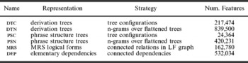
We create six different basic feature sets by using different representations and/or feature extraction strategies. These are summarised in Table 1. The precise details of these feature sets are not important here. What should be noted is that some sets have commonalities with others, either in the representation or strategy used. For example, dtc and dtn are based on derivation trees, and features are extracted for dtn and psn by flattening trees (e.g., as Lisp expressions) and taking n-grams (up to 4) over the node labels.
Basic feature sets. Each row gives the name of the feature set, which representation it is based on, its feature extraction strategy, and how many distinct features are extracted for the set from Redwoods 5

The six basic feature sets form the basis for constructing different LOPs. In particular, we focus on the three grouped feature sets listed in Table 2. all contains all six basic feature sets. The second group, div, contains the three basic feature sets that are most naturally diverse from one another. Their diversity comes from the fact that they use different representations and feature extraction strategies. The last group, sim, is constructed from the most similar three basic feature sets. Their similarity comes from the fact that dtn uses the same representation as dtc and the same feature extraction strategy as psn.
Grouped feature sets. Each line gives the name of the grouped set, which basic feature sets it is comprised of, and a brief characterisation of its nature

These grouped feature sets are used in two different ways. They can be used individually to specify different single models which are then combined together in a LOP, or they can be merged together (treated as a single feature set) and used for single models. When a grouped feature set is used as a single, merged feature set, we refer to a model which uses it as being monolithic. This is to suggest the idea that no internal structuring is imposed.
3 Parse selection models
Parse selection involves identifying the correct analysis for a sentence. Here we describe our parse selection models, which use the feature sets described previously. Throughout, f j(t) is the number of times feature j occurs in analysis t, λj is a weight, Z(s) is a normalisation factor for a sentence given its set of analyses τ = {t. . .}, and M k is a model.
3.1 Single models
As is standard for linguistically rich formalisms such as HPSG or LFG, we use log-linear models for modelling parse selection (Johnson et al. Reference Johnson, Geman, Cannon, Chi and Riezler1999). With such models, the conditional probability of an analysis t given a sentence s is:
(1)


This is a single model approach as the only feature set used is that of M k. The analysis with the highest probability is taken as the preferred one. Note that because the ERG usually produces relatively few parses for in-coverage sentences, they can be fully enumerated.
We use the implementation of the Limited Memory Variable Metric (LMVM) algorithm provided by the Toolkit for Advanced Discriminative ModelingFootnote 2 to determine the model weights (malouf Reference Malouf2002). Efficient training algorithms such as LMVM are crucial for a successful application of active learning which typically requires models to be estimated many hundreds of times. For example, a 10-fold active learning run with our data set and step sizes requires training each model over 350 times.
As is well known, it is usually beneficial to regularise the likelihood using a prior over the weights. Such priors contain free parameters which are typically set by optimising with held-out data. Within an active learning context, however, labelled data is scarce and therefore free parameters cannot be (easily or reliably) optimised in this manner. For our experiments, we thus use a Gaussian prior with a single variance of 1000 (and a zero mean) for all model weights. This may or may not be the optimal value. It represents a reasonable guess based on a good variance value for other tasks – this is meant to simulate the situation faced by a team developing models at the beginning of an actual active learning process. Even so, we find that this strategy easily outperforms unregularised models for our task.
Log-linear models most commonly form the basis for parse selection using rich unification grammars like DCGs (Osborne Reference Osborne2000), HPSG (Toutanova and Manning Reference Toutanova and Manning2002; Malouf and VanNoord Reference Malouf and van Noord2004) and Lexical Functional Grammar (Johnson et al. Reference Johnson, Geman, Cannon, Chi and Riezler1999; Riezler et al. Reference Riezler, Prescher, Kuhn and Johnson2000). Support Vector Machines (SVMs) provide an interesting alternative type of model. For example, using SVMs, Toutanova et al. (Reference Toutanova, Markova and Manning2004) obtained the highest reported accuracy for Redwoods 1.5 – though a log-linear model with the same features performed equivalently (Kristina Toutanova, p.c.). Using the SVMTorch II implementation (Collobert and Bengio Reference Collobert and Bengio2001), we found that SVMs with Gaussian kernels had comparable performance to log-linear models using the same features, but they took far longer to train: several hours on a given feature set rather than several minutes with LMVM. Using linear kernels provided faster training times (though still far slower than LMVM) and worse performance. Because of this, SVMs are less suitable for our active learning experiments, which require repeated retraining of models. In passing, we note that there is nothing restricting us to using log-linear models within the work described in this article. Any modelling technique that is probabilistic and allows for rapid retraining can be used. For example, we could use a log-linear model and a generative model. We could not use a LOP whose members used distance functions which were not on a similar scale (for example, using the margin of a SVM along with a probability from a log-linear model).
3.2 Logarithmic opinion pools
Ensemble learning is a general technique for improving system performance. Techniques such as bagging or boosting and other system combination methods have been shown to improve a variety of language technologies. When investigating the cost reductions from using techniques like active learning, is it thus important to consider ensemble models which may make more efficient use of the available data in the (possible) absence of sample selection with active learning. We create our ensemble model using the Logarithmic Opinion Pool (LOP) formulation (krogh and Vedelsby Reference Krogh, Vedelsby, Tesauro, Touretzky and Leen1995; Heskes Reference Heskes, Jordan, Kearns and Solla1998):
(2)
This is an ensemble approach as multiple models M 1,. . ., M n are employed. The normalising constant Z* simply ensures that the distribution over all parses sums to one. This is different from the per-model normalising constant Z(s) in equation (1). Each component model can have an associated weight w i which can be thought of as quantifying the contribution it makes to the decision making process. LOPs are related to and predate Products of Experts(Hinton Reference Hinton1999). Smith et al. (Reference Smith, Cohn and Osborne2005) applied LOPs to conditional random fields (CRFs) and found that they were competitive with regularized single model CRFs.
The weights w i balance the contribution each component model makes in prediction. Because the LOP is convex, these model weights can be set using a gradient-based search, much in the same way as for individual model parameters. The idea here is to treat each component model as a feature, with the value being the model's logarithmic probability of the data point in question. Fitting the resulting model maximises the likelihood of the data with respect to the whole opinion pool. Additionally these model weights can themselves be regularised. In our experience, simply setting the weights to uniform values (and not optimising them) generally yields excellent results and doing so also fits well within our data-poor active learning context. All of our LOPs therefore use uniform model weights.
LOPs have the following attractive property. Suppose Q is the true distribution and that P π is a LOP composed of the individual models P 1, P 2,. . . P n. Then:
(3)
Here K is the usual Kullback-Leibler divergence. This shows how LOPs can be factored into two parts. The E term reflects how close the component models are to the target model Q. The A term has no direct connection to the target model and instead describes the difference between the various component models. Since the Kullback-Leibler divergence is always non-negative, E ≥ A. Equation 3 also highlights the importance of model diversity. The more diverse the models, the greater A will be and (assuming E does not increase at a faster rate) the closer the LOP will be to the target model Q. Another interesting point is that an increase in E (how badly component models perform) can be tolerated so long as the increase in diversity is greater. Finally, note that smoothing the individual models (using for example a Gaussian prior) may reduce A since each model will become more similar to the uniform distribution and so more similar to each other.
The key to successfully constructing a LOP is therefore selection of a diverse set of models that have reasonable performance and, to a lesser extent, appropriate setting of the model weights w j. Returning to parse selection, we create LOPs from log-linear models. There are reasons why LOPs based upon log-linear models might outperform a corresponding monolithic log-linear model (one in which all distinct features are collapsed together into a single model which is trained in the usual manner). Preserving model diversity (as happens when individual log-linear models, with diverse feature sets, are trained in isolation and combined as a LOP) is provably beneficial. This property follows from the general discussion about LOPs and is experimentally verified later in this paper.
LOPs can have no hyperparameters to set. This makes them attractive when labelled data is scarce, as is the case in an active learning setting. Naturally, LOPs can also use priors at the component model level and at the LOP level.
4 Parse selection results
Section 2 outlined six basic feature sets and three grouped feature sets. Here, we show how well parse selection models using those feature sets perform when trained on all available material in Redwoods 5. Additionally, we show how well LOP parse selection models using diverse and non-diverse grouped feature sets perform and compare them to the corresponding monolithic models (which have access to all the same features). This will then set the scene for subsequent active learning experiments.
Parse selection accuracy is measured using exact match: a model is awarded a point only if it uniquely picks the analysis that is indicated as correct in Redwoods. To deal with ties, a model gets 1/m points when it ranks m parses highest and the best parse is one of them. Exact match is, of course, a much stricter measure of performance than those which evaluate the percentage of correct constituents or dependencies and thereby give partial credit for incorrect parses. The performance values we report were obtained from five runs of 10-fold cross-validation and are the averages of the performance across all folds. Significant differences are determined with a pair-wise t-test (p<0.05). All examples that have more than 100 parses were excluded from the training material (but not the test material). The baseline accuracy when choosing by chance is 20.9%.
Table 3 shows the single log-linear model parse selection results for both regularised and unregularised models. The name of each single model is ll, for log-linear, followed by the abbreviation of the feature set which it uses. All six models easily beat the chance baseline. The performance difference between all models pairs is significant except for that between the regularised and unregularised dtn models. The regularised dtc model is the highest performing single model using a basic feature set.
Parse selection results for single log-linear models using the basic feature sets. Performance is given both for models regularised with a Gaussian prior and for unregularised models. The baseline accuracy when selecting by chance is 20.9%

The particular performance figures are not especially important for present purposes – what matters more is that the models exhibit different performance characteristics from each other. This is an indication of their diversity, which, as noted in the previous section, is crucial for creating effective LOP models. A more direct characterisation of their diversity is the Spearman's rank correlation of a set of models on their predicted ranking of parses on unseen data: higher values mean that the models are more correlated with each other. For example, the rank correlation of the unregularised single models using the six feature sets of the all group is 0.72. For the sim group it is 0.81, whereas for the div group it is 0.67. This indicates that a LOP composed of models using the sim group will have a smaller A term (from equation (3)) than a LOP composed of the div group. These values were obtained by averaging over all pairwise correlations between models in a set.
Table 4 shows the performance of LOPs and monolithic models using the three grouped feature sets all, div, and sim. The LOP models are named as lop followed by the name of the feature group from which the component models are obtained. For example, lop-div uses ll-dtn, ll-psc, and ll-mrs as its component models. The component models themselves can be either regularised or unregularised. Regularisation for the LOPs in Table 4 indicates that the component models have been regularised, rather than the LOP itself. Since they are single log-linear models, the monolithic models are named as ll plus the name of the feature group which has been used to create the monolithic feature set. All differences of more than 0.1% between any two models are significant.
Parse selection results for LOP and monolithic models using the three grouped feature sets all, sim, and div. Here, regularised LOPs refer to regularisation of the component models of the LOPs rather than regularisation of the LOPs themselves

These figures demonstrate a number of important properties of LOP models. First, all of the unregularised LOP models easily beat the performance of corresponding unregularised monolithic models – without requiring any hyperparameters to do so. Second, the lop-all and lop-div models have performance which equals that of the corresponding regularised monolithic models, while, the lop-sim model performs significantly – though not drastically – worse than the regularised ll-sim model. This is a strong indication of the importance of diversity for optimal LOP performance.
There are two further relationships that provide evidence for the crucial role of diversity. First, lop-div's performance is equal to that of lop-sim, despite the fact that two of its component models, ll-mrs and ll-psc, are the worst models of all six basic models and that its best component model (ll-dtn) is less accurate than lop-sim's best component model (ll-dtc) (compare Table 4 with Table 3). Second, using regularised base models actually hurts LOP performance: compare 79.9% versus 80.8% for lop-all. This is a direct consequence of regularisation making the models more uniform and thus reducing the A term of equation (3).
Unregularised lop-all and regularised ll-all are the best performing models, at 80.8%. Thus, the LOP achieves equal performance to the regularised monolithic model without the need to set the variance hyperparameter for the prior. Later, the results from active learning show that this property of LOPs makes their performance more robust than that of corresponding monolithic models when the amount of training material varies.
Recall that these models use only examples with fewer than 100 analyses – this was necessary due to insufficient memory for training the monolithic ll-all (which has more than two million features). This limitation demonstrates a practical advantage of LOPs: each component model has a much smaller memory footprint and is trained individually. As such, LOP training can also be trivially parallelised. This allowed us to train an unregularised LOP which utilises all examples with up to 5000 analyses, leading to a significant improvement in performance: 81.3%.Footnote 3
On previous versions of Redwoods, a similar LOP (which used three component log-linear models trained from dtc, dtn, and a monolithic group set containing psn, mrs, and dep) was competitive with the highest reported performance for other models. Our active learning experiments are thus based on state-of-the-art models for the Redwoods parse selection task. For these experiments, we use the strongest configurations for both single and LOP models: regularised for the former and unregularised for the latter.
5 Active learning methods
A major cost in creating trainable speech and language technologies is the creation of labelled training material. In relatively simple domains such as text classification, unlabelled examples can usefully improve system performance, but the same has not been shown for more complex tasks such as semantic interpretation. Invariably, the more manually labelled training material available, the better the performance. A well-known result shows that labelled examples are worth an exponential number of unlabelled examples (castelli and Cover Reference Castelli and Cover1996). Given these facts, there is considerable interest in finding efficient ways of creating small, manually labelled training sets which lead to high system performance. Active learning is concerned with selecting such training sets.
The basis of (most) active learning is as follows. It is possible to show that the error rate of some model can be factored into two terms: its variance and bias (Geman et al. Reference Geman, Bienenstock and Doursat1992; Kohavi and Wolpert Reference Kohavi and Wolpert1996). Variance here means how much a model's predictions fluctuate according to the choice of training set. Bias means the systematic errors relative to a Bayes Optimal model. Labelling those examples which reduce either the bias or the variance will reduce the error of the model. The degree to which the bias or variance is reduced will in turn affect the rate by which the model's error will decrease.
If examples are selected for labelling using a strategy of minimising either variance or bias, then a model's error rate typically decreases much faster than if examples are selected randomly. Active learning methods attempt to identify such informative examples.
In this section, we describe the active learning methods that we tested on Redwoods 5, which include both single-model and ensemble-based active learning techniques. Our single-method approaches are not meant to be exhaustive. In principle, there is no reason why we could not have also tried (within a kernel-based environment) selecting examples by their distance to a separating hyperplane (Tong and Koller Reference Tong and Koller2000) or else using the computationally demanding approach of Roy and McCallum (Reference Roy and McCallum2001). However, the methods we use are all computationally tractable.
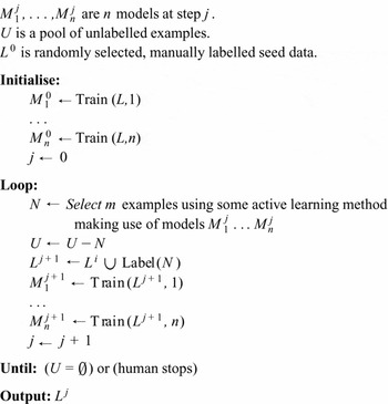
Figure 1 gives pseudo-code outlining how active learning is implemented. The active learning methods we use differ from each other only in how they select which examples should be labelled at each stage. The function Train(L, i) creates a model M i using feature set i and the labelled training set L. The function Label(N) means manually label the examples N. As can be seen, there is an initialisation phase, when the models are trained on an initial seed set of randomly selected examples. Random selection is the best way to carry out such initialisation. The reason for this is that active learning itself is an estimation task: learning which examples to label. With minimal labelled training data, active learning will be error-prone. With slightly more data, active learning will instead be able to select informative examples for labelling.
Pseudo-code for ensemble-based active learning.

After initialisation, there is a loop whereby examples are selected for labelling using a given active learning method and a corresponding set of models. Selected examples are then manually labelled and added to the training set. All the models are then retrained and the process continues. Our active learning approaches are therefore pool-based –we do not generate sentences nor do we sample sentences from some stream of examples. The end-result is a labelled training set L j.
Active learning for parse selection is potentially problematic as sentences vary both in length and the number of parses they have. After experimenting with, and without, a variety of normalisation strategies, we found that generally, there were no major differences overall. All of our methods therefore do not have any extra normalisation.
For all the methods that we now describe, τ denotes the set of analyses produced by the ERG for the sentence and M k is some model. ℳ is the set of models M 1. . .M n.
5.1 Uncertainty sampling
Uncertainty sampling is perhaps the most popular active learning method in the literature. The insight behind uncertainty sampling is that the degree of informativity of an example is proportional to how uncertain a model is when assigning a label. Uncertainty is naturally measured as entropy. For parse selection, the utility of an example is expressed as follows:
(4)
Higher values of f us(s, τ, M k) indicate examples on which the learner is more uncertain and thus presumably are more informative. Calculating f us is trivial with the conditional log-linear models described in section 3.
Uncertainty sampling as defined above is a single-model approach. It can be generalised to an ensemble by replacing the probability of a single log-linear model with that of a LOP:
(5)
Recall that ℳ is the set of models M 1. . .M n and P π is a LOP using those models. While this is still a single active learning method, it uses an ensemble parse selection method.
5.2 Lowest best probability selection
Uncertainty sampling considers the overall shape of a distribution to determine how confident a model is for a given example. A radically simpler way of determining the potential informativity of an example is simply to consider the absolute probability of the most highly ranked parse. The smaller this probability, the less confident the model is for that example and the more useful it will be to know its true label. We call this new method lowest best probability (LBP) selection, and calculate the score of an example as follows:
(6)
LBP can be extended for use with a LOP in the same manner as uncertainty sampling.
Note that when dealing with problems involving two labels, LBP and uncertainty sampling are equivalent. However, they can have very different biases for tasks with a variable number of labels, such as parse selection. For examples with a uniform distribution, f us increases with ambiguity and f lbp decreases, so both are biased toward more ambiguous examples. However, if one label is given more than half the probability mass, f us still increases while f lbp of course remains fixed. For example, a distribution with 100 labels where one label gets 70% of the mass and the others share the rest has a f us value of 2.9, which is greater than the f us values of uniform distributions with seven or fewer labels. Thus, selection according to f us can prefer examples for which there is a high degree of confidence for one label over examples which have uniform distributions, while selection by f lbp would be strongly biased toward more uniform examples in such cases.
Another difference is that LBP only needs to consider a single parse (per sentence). This can make it considerably more efficient than uncertainty sampling. For approaches which allow the Viterbi analysis to be efficiently recovered, active learning using LBP would require recovering just a single analysis. This is why LBP can be efficient. Within the context of log-linear-based parse selection, LBP could be implemented using a dynamic programming method for extracting features (Geman and Johnson Reference Geman and Johnson2002).
5.3 Fixed Query-by-Committee
Another active learning method we use is inspired by the query-by-committee (QBC) algorithm (Freund et al. Reference Freund, Seung, Shamir and Tishby1997; Argamon-Engelson and Dagan Reference Argamon-Engelson and Dagan1999). According to QBC, one should select data points when a group of models cannot agree as to the predicted label. The intuition here is that the variance of a model with respect to an example correlates with the degree with which the members of an ensemble disagree. QBC, like all ensemble methods, will only work if the individual models are not fully correlated with each other. When examples can take one of a variable number of labels (as is the case when labelling sentences with parse trees), QBC-based methods will tend to select examples with many possible labels. This follows simply from the fact that as the number of possible labels increases, then the chance that two models will both predict the same label will decrease.
Using a fixed committee consisting of n distinct models, the examples we select for annotation are those for which the models most disagree on the preferred parse. One way of measuring this is with vote entropy (Argamon-Engelson and Dagan Reference Argamon-Engelson and Dagan1999):Footnote 4
(7)
where V(t, s) is the number of committee members that prefer parse t. QBC is inherently an ensemble-based method. We use a fixed set of models in our committee and refer to the resulting sample selection method as fixed QBC. Clearly there are many other possibilities for creating our ensemble, such as sampling from the set of all possible models.
6 Experimental methodology
Active learning research typically involves hundreds of experiments, and it is simply not viable to have humans label data that many times. Instead, simulation studies are invariably used. Here, to test the effectiveness of the various active learning strategies discussed in the previous section, we simulate the annotation of Redwoods 5, varying both the models and the methods for each experiment. This is in line with almost all active learning research. Our primary goals are to compare (a) the effectiveness of the three methods – uncertainty sampling, LBP sampling, and QBC – to each other on each model, and (b) LOP models against monolithic parse selection models when used in an active learning setting. Our primary concern is active learning for parse selection, but later we also consider text classification to show the generality of our results.
For all experiments, we used two runs of 10-fold cross-validation. Each fold begins with 25 randomly chosen, manually annotated seed sentences. At each round, new examples are selected for annotation from a randomly chosen, fixed sized 500 sentence subset according to the method until the annotated training material made available to the learners contains at least 8000 examples and 25,000 discriminants.Footnote 5 Our selection size for manual annotation starts with 25 examples at each round and is doubled at 500, 1000, 2000, and 4000 examples. Finally, all examples with more than 100 parses are excluded from labelling.Footnote 6
6.1 Cost metrics
When evaluating the effectiveness of (simulated) active learning methods, it is crucial to define a cost metric that correlates with the actual human effort of annotating examples as accurately as possible. In many domains, the cost of annotating each unit, or example, is essentially the same for all examples. For parsing, on the other hand, different sentences can require drastically different amounts of effort to annotate. Assuming that each sentence entails the same labelling cost will not adequately reflect the effectiveness of active learning applied to it. Even so, Tang et al. (Reference Tang, Luo and Roukos2002) present their results for using active learning to create material for parsing in terms of a unit cost per sentence. Hwa (Reference Hwa2000) instead counts the number of brackets (constituents) in the parse trees to reflect that fact that larger trees take more effort to create than smaller ones. This approach more realistically reflects the variable nature of labelling sentences. However, it assumes annotation involves labelling all constituents in a tree.
The way Redwoods examples are annotated provides the basis of an alternative cost metric for quantifying labelling effort. Compared to inspecting all parses to identify the correct one, this approach is much more efficient at labelling the correct parse, as typically only a few decisions are necessary. Crucially, this approach varies with the ambiguity of the sentence (unlike a unit cost per sentence) and also does not mean wasting labelling effort on trees which can be deterministically created (unlike counting all constituents in a tree). This metric comes in the form of discriminants: simple properties of derivation trees that distinguish competing analyses and are relatively easy to judge (Oepen et al. Reference Oepen, Toutanova, Shieber, Manning, Flickinger and Brants2002). An example of a discriminant is one which declares that a particular prepositional phrase attaches to a noun phrase – setting this to true immediately excludes all parses in which the prepositional phrase attaches elsewhere, such as to the verb phrase.
During annotation, the annotator selects discriminants one at a time and marks them as true or false properties which the correct parse should have. Each discriminant thus allows entire subsets of incorrect parses to be removed from consideration at each step, and the correct parse is eventually singled out. As such, the annotator does not need to inspect all parses, and so parses are narrowed down quickly (usually exponentially so) even for sentences with a large number of parses. The cost of annotating an example in Redwoods is thus relative to the number of possible parses, rather than the number of constituents in a parse. More specifically, the number of discriminant decisions necessary to annotate a sentence is proportional to the log of the number of its parses (Tanaka et al. Reference Tanaka, Bond, Oepen and Fujita2005). This approach to disambiguation was first used by Carter (Reference Carter1997), who used it when creating training material for the Core Language Engine.
Data about which discriminants were selected during the annotation of each sentence is recorded in Redwoods. Typically, more ambiguous sentences require more discriminant values to be set, reflecting the extra effort put into identifying the best parse. Since the Redwoods treebank uses discriminants when specifying the correct analysis, it is natural to use them as the basis of calculating annotation cost for active learning experiments with Redwoods parse selection models. For Redwoods 5, annotators required between 1 to 15 discriminants (avg. 3.1) to identify the correct analysis of a sentence.
Active learning is fundamentally concerned with minimising the labour costs associated with creating labelled datasets. Despite the direct use of discriminants in Redwoods annotation, the cost of annotation is only truly measured in terms of timing. There is therefore a need to ground discriminant cost – or any simulated annotation cost metric for that matter – in terms of actual timing. This information is not available for Redwoods 5, but fortunately Redwoods 1 does have timing information associated with each sentence.Footnote 7 It is thus possible to gauge how long an example really took to label.
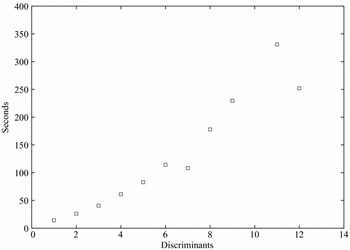
This information allowed us to verify whether discriminant cost is indeed in line with how long it really takes to label examples.Footnote 8Figure 2 is a plot of the average number of seconds taken to annotate an example with a given number of discriminants. It shows that there is a strong linear correlation between the two variables (Pearson's r=0.95). Clearly, discriminant cost is a superior approximation of the true cost than unit cost, which would treat all examples alike. Since active learning methods often choose more ambiguous examples –which typically require more time to annotate– than random sampling, unit cost would thereby overstate the gains from active learning. We have found this to be the case in our experiments: unit cost always reports larger cost savings than discriminant cost.
Plot showing a linear correlation (Pearson's r=0.95) of the average number of seconds annotators needed to label examples with a given number of discriminants.

Ngai and Yarowsky (Reference Ngai and Yarowsky2000) carried out active learning experiments using time as their metric and comparing QBC with sequential sampling and with manual rule writing. They found that QBC was more time efficient than sequential sampling, thereby confirming their particular annotation costing assumptions. Their domain was base noun phrase chunking, which is considerably simpler than HPSG parse selection.
Although we have not measured the cognitive burden on humans, we strongly believe that simply selecting the best parse is far more efficient than drawing the best parse for some sentence (as exemplified by Hwa (Reference Hwa2000). However, an interesting tension here is that Redwoods annotation is committed to the ERG producing the intended parse within the set of analyses. When drawing a parse tree, by definition, the best parse is created. This may not be always true when using a manually written grammar such as the ERG.
6.2 Comparing active learning methods
Having determined a representative cost for labelling different examples, there are various ways for measuring the overall effectiveness of active learning. The most common approach is to consider the annotation cost savings compared with another selection method.
For this, we use two strategies which highlight different aspects of the task. The first approach, called the data utilisation ratio (DUR), quantifies how much data needs to be labelled in order for a model and method to reach the performance level of the same model using random sampling (Abe and Mamitsuka Reference Abe and Mamitsuka1998; Melville and Mooney Reference Melville and Mooney2004). In order to better compare the DURs across various models – each with their own maximal accuracy – we consider the DURs for reaching 80%, 85%, 90%, 95%, 99%, and 100% of full accuracy. For example, for the regularised ll-dtn model, which has a maximal accuracy of 77.2%, we collect the DURs for the following accuracy levels: 61.8%, 65.6%, 69.5, 73.3%, 76.4%, and 77.2%. The DUR provides a fine-grained characterisation of the performance of active learning methods as more data is selected and of their robustness throughout the entire sample selection process.
The second approach assumes that the annotation cost is fixed at some amount and measures the predictive ability of different model and method systems with the labelled data. This can be measured with the percentage error reduction (PER) averaged over points on the learning curve (Saar-Tsechansky Provost Reference Saar-Tsechansky and Provost2004; Melville and Mooney Reference Melville and Mooney2004). Because the models for many of their datasets reach full accuracy with a relatively small amount of all available data (even randomly sampled), Melville and Mooney (Reference Melville and Mooney2004) average only over the 20% of points where the largest improvements are produced. For Redwoods, random sampling only achieves full accuracy when it has all available material; thus, we compare points from the beginning of sample selection until all active learning methods are guaranteed to reach their performance ceiling: this is roughly two-thirds of all available discriminants. We thus obtain an average PER between two curves by measuring the PER for every 1000 discriminants, starting at 1000 discriminants and ending at 20,000.Footnote 9 Statistical significance for an average PER is determined with a paired t-test (p < 0.05) on the difference in performance of the two systems averaged across the selected points.
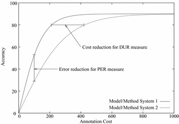
Figure 3 graphically shows how the measurements are taken for the DUR and PER measures for two hypothetical learning curves. DUR quantifies the cost difference between two curves, and PER quantifies their performance difference.
Learning curves for two hypothetical method/model systems showing how the measurements for DUR and PER are taken. Here, system 1 demonstrates better performance.

7 Active learning results
In this section, we present our main results. We begin with random sampling results, comparing single and LOP models. We then show active learning results, both for single models and LOPS using our various active learning methods. For completeness, we conclude by demonstrating that that random sampling is a stronger baseline than other model-free selection methods, such as sequential sampling.
All single/monolithic models in these experiments are regularised with a Gaussian prior; all LOPs use unregularised component models. These are the strongest configurations for both model types – see section 4 for details.
7.1 Random sampling with single and LOP models
Our baselines are those produced by random sampling for all models – these form the basis of comparison against the various active learning methods. However, they can also be used to compare the performance of different models trained on varying amounts of data by using the average PER measure. Table 5 shows the average PERs for monolithic and LOP models using the combined feature sets compared to regularised ll-dtc, which is the best basic model. The monolithic models show that the extra features in the grouped feature sets always help, even when simply concatenated together as a monolithic feature set. The LOP models show that the diverse grouped feature sets all and div provide further error reductions over their monolithic counterparts. However, the LOP using the less diverse sim group does not provide as much of an improvement as the monolithic model.
Percentage error reductions for LOP and regularised monolithic models using all, div, and sim compared to regularised ll-dtc, all using random sampling

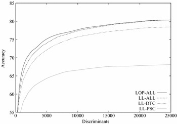
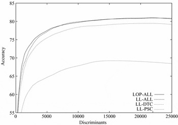
The higher PER s of lop-all and lop-div over lop-dtc is due to their superiority with less data. This can be seen from examining the full learning curves. For example, Figure 4 shows the performance of both lop-all and ll-Mall. This graph shows that the LOP is superior until roughly 15,000 discriminants: a small but statistically significant PER of 2.0% over ll-all. This can be attributed to how the prior was set for the monolith – we assumed a single value for the variance that works better for more data and is thus possibly sub-optimal early on. This demonstrates the attractiveness of the LOP formulation for active learning for tasks which can be broken into diverse views. It does not rely on careful setting of hyperparameters like the Gaussian variance and thus delivers higher performance throughout the sample selection process. This is especially important when there is insufficient data to provide a held-out set for optimising the hyperparameters.
Learning curves for random sampling with lop-all, ll-all, ll-dtc, and ll-psc.

Figure 4 also shows the learning curves for random sampling with ll-dtc and ll-psc. This demonstrates the consistent superiority of both lop-all and ll-all compared to ll-dtc (the best single model using a basic feature set) and the massive error reductions of all three of these models to ll-psc (the worst single model). In addition to its lower accuracy, note how the rate of increase for ll-psc is also much lower than that of the other models. Better modelling, especially using a LOP or a regularised monolithic model, yields better performance and achieves it more quickly than simpler models.
7.2 Single-model active learning results
Since QBC is inherently an ensemble-based active learning method, only uncertainty and LBP sampling can be used by single models. Figure 5 shows overall learning curves for ll-all with these two methods and random sampling. As can be seen, both methods are superior to random sampling throughout the entire sample selection process and LBP is marginally superior to uncertainty early on.
Learning curves for ll-all using random, uncertainty, and LBP sampling.

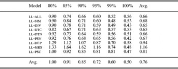
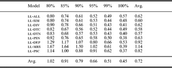
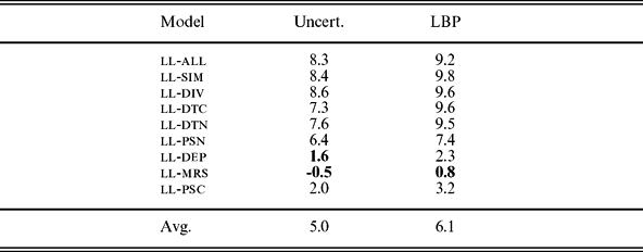
To concisely show the trends for all models, we use the DUR and PER measures discussed in section 6.2. Tables 6 and 7 show the DURs for each single model using uncertainty and LBP sampling, respectively. The values are given for each of the six relative performance levels (relative to each model's performance when using all material), and are averaged for each model and performance level. The models are listed in order of descending parse selection performance. Several observations can be drawn from these tables:
• Active learning is rarely less efficient than random sampling. This can be clearly seen in that for almost every model, the DUR values are less than one (i.e., when fixing the model and comparing an active learning method against random sampling).
• Active learning can actually be less efficient than random sampling for weak models (see ll-mrs and ll-dep).
• LBP sampling performs slightly better than uncertainty sampling, especially when used with better models. This can be partially explained by the fact LBP attends to the probability only of a single label, whereas uncertainty considers the entire distribution and hence is more sensitive than LBP to a weak model's poor estimates.
• Better models provide better relative active learning performance. This can be seen not only by comparing the DURs of the different models, but also by the progressive improvements in data utilisation for each model as they near their full accuracy. In particular, note the average values. Recall that each DUR is determined from a model's own random baseline, so these models deliver better relative performance even though their baselines are considerably higher than those of the weaker models.
One thing these DUR values do not show is that the better models also deliver better absolute performance – see section 7.3 and in particular Figure 7 for details on this.
Data utilisation ratios of single model uncertainty sampling compared to random sampling to reach given percentages of maximal accuracy

Data utilisation ratios of single model LBP sampling compared to random sampling to reach given percentages of maximal accuracy

One clear exception to the better-models-equals-better-utilisation trend is ll-psc, which exhibits better active learning performance than ll-mrs and ll-dep despite having overall worse parse selection performance than either. The poor data utilisation for ll-mrs and ll-dep can in part be attributed to spurious ambiguity in the grammar. This causes many examples to have “incorrect” analyses that have identical logical forms and dependencies to the one identified as correct. That means that such examples are very likely to be chosen according to uncertainty or LBP sampling by these models and yet they will provide less discriminating information for them because the same representation is indicated as both correct and incorrect. So, if our evaluation was based on obtaining only the correct logical form, the observed degradation would not necessarily be as great.
As an alternative view on the effectiveness of the two active learning methods, Table 8 shows the average PERs for each model and method compared to the same model using random sampling. As with the DUR measure, the PER results show that better models provide better active learning performance and that LBP sampling is significantly better than uncertainty sampling. The difference between LBP and uncertainty according to PER is more marked than for DUR. This is because we sampled more points early in the sample selection process for PER, where LBP had the largest gains (e.g., see Figure 5). Also, we sampled more points for PER than for DUR, so the PER values provide a more representative overall average of active learning performance.
Percentage error reductions for single model uncertainty and LBP sampling compared to random sampling. All values are statistically significant except those in bold
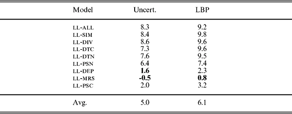
One of the advantages of the PER measure is that it uses absolute reference points (the number of discriminants annotated rather than DUR's relative performance values) – this allows different model/method systems to be directly compared, such as a better modelling strategy versus an active learning strategy for improving performance. For example, ll-dtc using LBP sampling provides a significant 2.6% reduction over ll-all using random sampling. However, it does not provide a significant reduction over lop-all using random sampling: the two combinations are equivalent in their effectiveness for using the annotated material. The rest of the basic models using active learning are easily beaten by lop-all using random sampling. These results show that the common practice in active learning of using the convergence results of a single model, trained using random sampling, can be misleading: we can improve upon the performance of a single model without using active learning by using an ensemble model.
7.3 LOP active learning results
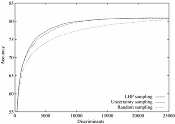
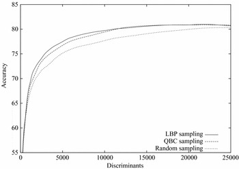
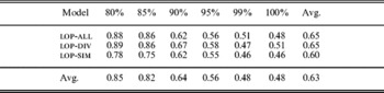
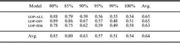
Figure 6 shows overall learning curves for lop-all with LBP, QBC (with a committee formed of lop-all's component models) and random sampling (the curve for uncertainty sampling is essentially the same as that for LBP and so is left out). Both methods are superior to random sampling throughout the entire sample selection process and LBP, along with uncertainty, is superior to QBC – especially early on. These trends also hold for the other LOPs. Tables 9, 10 and 11 show the DUR s for the different LOP models using uncertainty, LBP, and QBC sampling, respectively.
Learning curves for lop-all using random, QBC, and LBP sampling.

Data utilisation ratios of LOP uncertainty sampling compared to random sampling to reach given percentages of maximal accuracy

Data utilisation ratios of LOP LBP sampling compared to random sampling to reach given percentages of maximal accuracy

Data utilisation ratios of LOP QBC sampling compared to random sampling to reach given percentages of maximal accuracy

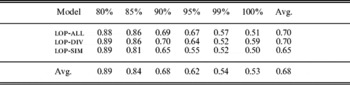
One observation that can be made from these results is that the DURs of LOP models using uncertainty sampling are marginally better than those of their corresponding monoliths. This is especially notable since LOPs have higher random baselines against which they are evaluated (e.g., compare the difference between ll-all and ll-all in Figure 4).
Second, the DURs of LOP models using LBP sampling are worse than those of the corresponding monoliths. However, because they are compared to a higher baseline, they are equivalent in absolute terms except for the sim models, where the monolithic model easily beats the LOP. Again, we see that diversity is crucial for LOP performance.
There is little to differentiate uncertainty sampling and LBP sampling for LOPs. However, QBC clearly delivers poorer data utilisation than either. QBC is very sensitive to the quality of the individual committee members – for example, two components models of lop-div are ll-dep and ll-mrs, which are the two worst single models. These models plus ll-psc also contribute to poor QBC performance for ll-all. However, lop-sim contains the three best single models (ll-dtc, ll-dtn, and ll-psn); accordingly, QBC works better for lop-sim than the other LOPs – though still not as well as uncertainty or LBP. In addition to QBC's sensitivity to committee member performance, it also has a stronger bias for selecting more ambiguous sentences – which generally cost more to annotate – than either of the two other methods.
The PERs for the LOPs are given in Table 12. This metric confirms the similar performance of uncertainty and LBP sampling for our LOPs and their superiority to QBC.
LOP models: percentage error reductions for active learning methods compared to random sampling to reach given percentages of maximal accuracy
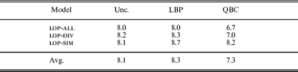
In absolute terms, the best configuration is lop-all using either uncertainty or LBP sampling. Compared to the best monolithic model configuration (ll-all with LBP) lop-all with LBP provides a small but significant PER of .7%. Figure 7 provides the full learning curves for various models using LBP sampling. This shows that the models retain the same relative positions to each other as for random sampling (see Figure 4) and that lop-all with active learning provides the best overall performance.
Learning curves for LBP sampling with lop-all, ll-all, ll-dtc and ll-psc.

7.4 Ad hoc selection results
Active learning is not the only way to determine which sentences should be labelled. Other than using random sampling, it is also instructive to consider some parsing-specific strategies that are model-free. Since sentences have variable length and ambiguity, there are four obvious selection metrics that make no use of active learning methods: select sentences that are longer, shorter, more ambiguous or less ambiguous. We tested all four ad-hoc selection methods using all of our models together and found not a single method which improved upon random sampling with the same model. It is also important to consider sequential selection, which is a default strategy typically adopted by annotators for many domains.
Table 13 shows the results of testing lop-all with sequential sampling and sampling by shorter sentences and longer sentences. Sampling by lower and higher ambiguity was for the most part on par with sampling by shorter and longer sentences, respectively. Selecting longer sentences is the most effective of these but is still far worse than random sampling.
Data utilisation ratios of lop-all using ad hoc selection methods compared to random sampling

The poor performance of sequential selection can be partially attributed to the fact that Redwoods 5 contains three different domains contained in sequential sections. Because of this, sequential selection does not choose examples from the latter domains until all those from the first have been selected. It thus only sees examples that are similar to those in the test set from the latter domain after many selection rounds.
8 Active learning for text classification
The active learning results presented in the previous section all concerned labelling data for Redwoods. An interesting question is whether the results carry over to other tasks – especially those for which it is more difficult to construct diverse feature sets. To investigate this, we considered labelling data for the classic text classification exercise. Active learning has already been applied for text classification: Lewis and Gale (Reference Lewis and Gale1994) showed that uncertainty sampling outperformed random sampling on many data sets, and McCallum and Nigam (Reference McCallum and Nigam1998) found that QBC also outperformed random sampling. Note that we are not concerned with an exhaustive comparison of active learning applied to text classification.
Our text classification experiments were setup as follows. We used the Reuters 21578 distribution 1.0, which has 13k articles and 135 labels. It was divided into the standard ‘ModApte’ split (9.6k training examples and 3.3k test documents). Additionally, we only used documents that had a single label and also only used labels that were used in at least one training and one testing document. This resulted in the following eight labels: acq crude earn grain interest money-fx ship trade. As such, there were 5485 documents in the training set and 2189 in the testing set. Each document was truncated to the first 100 distinct words (including stop-words). Documents shorter than 100 words were padded with dummy words. Evaluation was in terms of exact match: a model gets a point for guessing the correct label of a document, otherwise it gets nothing.
Unlike the HPSG parse selection task, this task has no natural feature split. We constructed one feature set, tc-word, using features which consisted of a word and the document label. All words were used for features, with no cutoff. Another feature set, tc-stem, consisted of the same set of word-label pairs, except that words were stemmed (using the Porter stemmer). The final feature set, tc-all, was the union of both of these feature sets.
As with the parse selection models, we used single log-linear models for all of the feature sets and a LOP for tc-all (so this LOP used just two component models, based on tc-word and tc-stem). During active learning, all unlabelled documents were considered for selection. Each model/method system was run ten times using a randomly selected 100 document seed set each time and continued until all material had been selected. The step size for each run began at five documents and was increased by 20 after every 10 rounds.
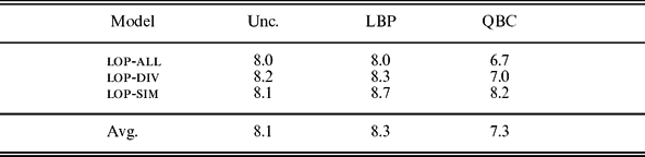
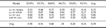
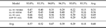
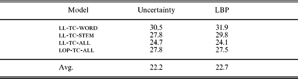
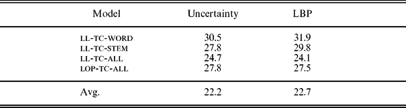
Tables 14 and 15 show the DURs, compared to random sampling, for the different models using uncertainty and LBP sampling, respectively. Unlike the parse selection results, we give DURs for absolute, rather than relative, levels of accuracy. This is because all the different models achieve the same overall accuracy of 95.5% and because the models achieve high levels of accuracy very quickly (already roughly 80% with the initial 100 documents). In line with previous results for active learning for text classification, the active learning methods achieve very large reductions over random sampling in the number of labelled documents necessary to reach given levels of accuracy. Overall, LBP performs similarly to uncertainty sampling, thereby confirming our parse selection results for another domain.
Data utilisation ratios of single model uncertainty sampling compared to random sampling to reach given performance levels (n.b.: these are absolute performance values, not relative ones as with the parse selection DURs)

Data utilisation ratios of single model LBP sampling compared to random sampling to reach given performance levels (n.b.: these are absolute performance values, not relative ones as with the parse selection DURs)

A notable difference is that ll-tc-word and ll-tc-stem have much lower DURs than ll-tc-all and lop-tc-all. The former models have lower baselines with random sampling than the latter models, and they make up some of the difference with active learning. In absolute terms, ll-tc-all and lop-tc-all have superior performance both with and without active learning.
ll-tc-all is slightly more efficient than lop-tc-all when random sampling is used, but there is little to differentiate the two models with active learning. This suggests that while LOP models can be interesting alternatives to traditional monolithic models, they are most effective when the feature sets are diverse, such as those we use for parse selection.
For completeness, we give the PERs for text classification active learning in Table 16. These simply confirm the similarity in performance between uncertainty and LBP sampling for this domain. In summary, these text classification results show that LBP can continue to produce similar results to uncertainty sampling, even though using a different domain to parse selection. The LOP results are encouraging in that even though the domain does not directly support naturally diverse feature sets, a LOP with non-diverse component models remains on par with a corresponding single model.
Percentage error reductions for uncertainty and LBP sampling compared to random sampling for text classification. All reductions are significant
9 Related work
There is a large body of active learning work in the machine learning literature, but less within natural language processing. There is even less work on ensemble-based active learning. Baram et al. (Reference Baram, El-Yaniv and Luz2003) consider selection of individual active learning methods at run-time, but their active learning methods are only based on single model approaches. The QBC approach to active learning is clearly closely related (seung et al. Reference Seung, Opper and Sompolinsky1992). Melville and Mooney (Reference Melville and Mooney2004) discuss an approach called Active-Decorate that develops a diverse committee from a single model and selects new examples with QBC-based methods. It would be interesting to consider whether using the resulting committees in a LOP and selecting according to LOP uncertainty or LBP sampling would improve on their results.
For parsing, Thompson et al. (Reference Thompson, Califf and Mooney1999) achieved a 29% reduction in annotation using (single model) uncertainty sampling. Hwa (Reference Hwa2000) also applied uncertainty sampling for parser induction. Tang et al. (Reference Tang, Luo and Roukos2002) managed to achieve a 60% reduction,Footnote 10 yet again using uncertainty sampling, along with a computationally demanding clustering strategy. In all cases, only relatively simple parsers were used, and also, comparison was with a single model, trained using random selection. Hwa et al. (Reference Hwa, Osborne, Sarkar and Steedman2003) showed that for parsers, active learning outperforms the closely related co-training, and that some of the labelling could be automated. However, their approach requires strict independence assumptions.
10 Discussion
For building complex language systems, the ability to create concise, informative training material is obviously attractive. We have shown that both active learning and ensemble modelling support the creation of such training sets. The benefits obtained from these methods are additive: using both strategies together provides additional cost reductions. Logarithmic opinion pools are very simple, and we expect that greater savings might follow by combining them with more complex ensemble model techniques such as boosting.
Unlabelled data could also be beneficial. Future work should consider generative models when reranking HPSG parses, as those models can potentially benefit from unlabelled data. Discriminative (log-linear) models ignore the probability of the data and cannot so easily be usefully constrained by it. We are however skeptical that significant performance boosts will come from unlabelled data: manually labelling data is a much surer path to success.
We have not dealt with outliers. Within our domain, there are no outliers as such and so this is not a problem. When dealing with other noisy domains (for example, gathering examples from the Web) then extra steps will need to be taken. In passing, we note that ensemble models are more resistant to noise than single models (Osborne Reference Osborne2002). Future work should therefore consider whether ensemble-based active learning is also noise-resistant.
Frequently in active learning there is an assumption that labelling is a one-off exercise. When there is uncertainty about the task, or new developments in machine learning emerge, there is then a question about the value of previously labelled data. The key to successful reuse of data created using active learning hinges on the relationship between the model used to select examples for labelling and the model that is reusing that data An open question is whether it is possible to create labelled data which is useful for most models, rather than being tuned to the needs of a single model (Baldridge and Osborne Reference Baldridge and Osborne2004)
Acknowledgments
We would like to thank Markus Becker, Steve Clark, and the anonymous reviewers for their comments. Jeremiah Crim developed some of the feature extraction strategies and code, and Alex Lascarides made suggestions for the semantic features. This work was supported by Edinburgh-Stanford Link R36763, ROSIE project.