2.1 The basic model settings

Consumers are risk-neutral with no saving. Her instantaneous utility is given by

(1) \begin{equation} U=e^{\frac{1}{J}\int _{0}^{J}\ln Y_{j}dj},\qquad J\geq 1 \end{equation}

where $Y_{j}$ is differentiated final output $j$ . We assume that $Y_{j}$ is competitively produced with a continuum of intermediate goods $y_{ji}$ according to

(2) \begin{equation} \ln Y_{j}=\int _{0}^{1}\ln q_{ji}y_{ji}di,\qquad q_{ji}=\lambda ^{k_{ji}},\quad \lambda \gt 1,\quad k_{ji}=0,1,2,\ldots \end{equation}

where $q_{ji}$ is the quality level of $y_{ji}$ . Intermediate product firms conduct R&D to increase $k_{ji}$ , and the highest quality products are always used for final output production. Quality innovations allow monopoly firms to produce some intermediate goods and earn profits. In this section, we use $\pi$ to denote (net) profit per intermediate product and take $\pi$ as given.

Figure 2.

If an entrepreneur succeeds in entrant R&D, she starts with $h_{i}$ number of monopoly goods in intermediate good industry $i$ . After entry the entrepreneur generates further innovation as an incumbent.

Consider Fig. 2. The horizontal axis shows the index of final output, and that of intermediate products is on the vertical axis. Each point in the figure identifies an intermediate good $y_{ji}$ used to produce final output $Y_{j}$ . The production function (2) means that producing final output $j$ requires a range of intermediate products, indicated by a vertical dotted line $I_{j}=\left \{ 0\leq i\leq 1|j\right \}$ . We assume that those intermediate goods in $I_{j}$ are specific to $Y_{j}$ and cannot be used for other final output $Y_{j^{\prime }}$ , $j^{\prime }\ne j$ . In addition, $y_{ji}$ is a different product from $y_{j^{\prime }i}$ , $j^{\prime }\ne j$ , hence their quality improvement requires separate successful innovations.

Now let us turn to an intermediate product industry $i$ where some goods are competitively produced and others are produced by a single monopoly firm, run by an entrepreneur. The state of each good, taht is competitive or monopoly, is determined by a process of innovation and product obsolescence, as explained later. A monopoly firm initially produces a continuum of $h_{i}\lt J$ products when it enters an industry $i$ after successful entrant R&D (replacing a previous incumbent firm). All other products in $i$ are competitively produced (more explanation on the entry/exit process through creative destruction later). After entry, a firm conducts R&D to further increase the quality of competitive products in $i$ to become their sole producer. Research activities after entry are termed incumbent R&D. Let us use $n_{i}$ to denote that number of products the firm produces in $i$ . It is equivalent to

(3) \begin{equation} n_{i}=h_{i}+m_{i} \end{equation}

which consists of $h_{i}$ and $m_{i}$ , the latter of which is materialized through incumbent R&D. We also use $c_{i}$ to denote the remaining competitive goods in $i$ .

To introduce a Pareto distribution of profits in this otherwise standard Schumpeterian model, we use an insight of Klette and Kortum (Reference Klette and Kortum2004) that $m_{i}$ can be treated as countable, that is $m_{i}=0,1,2,3,\cdots$ in a continuum of product space in $i$ . Countability of $m_{i}$ has two implications. First, there are infinitely many products that are potentially produced by monopoly, no matter how large it is. Second, “most” of products in $i$ are competitively produced. The state of a firm in industry $i$ is completely characterized by $n_{i}$ . Indeed, some monopoly firms are lucky enough to produce an exceptionally large number of products, earning overly huge profits. This is one of the prominent features necessary to generate a Pareto distribution.

Let $N$ denote the number of monopoly products in the economy as a whole. Similarly, the number of competitive products across all intermediate goods industries is given by $C$ . Then, $N=\int _{i\in \Xi _{i}}n_{i}di$ and $C=\int _{i\in \Xi _{i}}c_{i}di$ , $\Xi _{i}\in \left \{ 0\leq j\leq J|i\right \}$ , hold. Given that a single monopoly firm produces multiple products in each intermediate industry, $N$ is equivalent to the average number of products produced by monopoly firms.Footnote ⁹ We also require

(4) \begin{equation} J=C+N. \end{equation}

Note that $n_{i}$ can be exceptionally large to generate a Pareto distribution and this feature is accommodated in (4) because the average of $n_{i}$ is finite, as will be established.

The economy is characterized by a turnover of monopoly firms through entry/exit, caused by creative destruction of intermediate products. Consider potential entrant firms conducting R&D. We assume that an entrant R&D success follows a Poisson process with an arrival rate of $g_{E}$ , which is taken as given in this section. It is undirected in the sense that an industry is randomly chosen from $i\in [0,1 ]$ to implement successful innovation. This assumption simplifies analysis, but it also captures in a simple way an unpredictable nature of R&D outcomes.Footnote ¹⁰ To introduce a drastic nature of creative destruction, we assume that all of the previous incumbent products in $i$ are rendered obsolete by entrant innovation in the same intermediate industry.Footnote ¹¹ The “death” of firms due to entrant R&D is the contracting force of the income distribution. A successful entrant in turn increases the quality level of a continuum of $h_{i}$ products by a factor $\lambda$ . We assume that $h_{i}$ products are randomly allocated to entrant firms.Footnote ¹²

In exposition that follows, we proceed in two steps regarding the assumptions of $h_{i}$ . Initially, we assume that the value of $h_{i}$ is assumed to be constant for all intermediate goods industries, though its location in Fig. 2 is random. We will establish that a profit income follows a Pareto distribution with a single right tail. In the second step, the Pareto distribution in the first step is interpreted as the right part of the entire distribution. The left part arises once the value (or the length) of $h_{i}$ is allowed to randomly change in addition to its random location in the figure. Before exploring the assumptions of $h_{i}$ , we turn to incumbent R&D.

After entry, incumbent firms engage in R&D to improve quality of competitive goods in their own industries. Incumbent R&D in industry $i$ makes it possible to expand the portfolio of the firm’s products stochastically with the Poisson arrival rate of $g_{I}$ per product. In this section, we take $g_{I}$ as given. The “per product” assumption plays a crucial role in generating a Pareto distribution in the right tail. To illustrate this point, consider an incumbent firm with $n_{i}$ products. The arrival rate of incumbent innovation is now given byFootnote ¹³

(5) \begin{equation} g_{I}n_{i}. \end{equation}

Its salient feature is that the more products are improved in quality, the higher the arrival rate of an additional innovation. This is the expanding force of the profit distribution.

There are two things worth mention regarding the assumption (5). First, the rate of innovation is different across $i$ . Initially, incumbent innovation occurs at a lower rate because $n_{i}$ is low. But as more and more innovations are generated, income growth accelerates. This result is consistent with the finding of Piketty et al. (Reference Piketty, Saez and Zucman2018) who show that the average annual growth of income is increasing in income percentiles in the US in 1980–2014 with a growth rate accelerating above the top 1%.Footnote ¹⁴ Second, as we will establish, the number of products $n_{i}$ is distributed according to a double-Pareto distribution in equilibrium, and hence so is $g_{I}n_{i}$ . This is in line with Guvenen et al. (Reference Guvenen, Karahan, Ozkan and Song2015) which show that growth of earnings is double-Pareto distributed, using a large U.S. panel data set. Third, the assumption also captures heterogeneity of firm growth among, stressed by Luttmer (Reference Luttmer2011) and Gabaix et al. (Reference Gabaix, Lasry, Lions and Moll2016).

2.2 Step 1: a constant ${\overline{\boldsymbol{h}}}$

Taking $\pi$ as given, define

(6) \begin{equation} z_{i}=n_{i}\pi \end{equation}

as the total (net) profit earned by an entrepreneur in an intermediate good industry $i$ . Step 1 assumes $h_{i}=\overline{h}$ , $\forall i$ . Then, define

(7) \begin{equation} \overline{z}=\overline{h}\pi . \end{equation}

All entrant firms start from the initial profit $\overline{z}$ . After entry, firms engage in R&D to increase the range of products they produce according to (5). Whenever innovation occurs, the total profit increases by $\pi$ , and its expected increase during $\Delta t$ is given by

(8) \begin{equation} \Delta z_{i}=\pi \left \{ 1\times n_{i}g_{I}\Delta t+0\times n_{i}\left (1-g_{I}\Delta t\right )\right \} =z_{i}g_{I}\Delta t. \end{equation}

It shows that total profit geometrically grows and can be very large. In Fig. 3, (8) corresponds to the rightward movement of an entrepreneur, as indicated by the arrow (1). On the other hand, there is always a possibility that entrant innovation occurs, replacing incumbents, which is captured by the arrow (2) in the figure.

Figure 3.

The right distribution of entrepreneurial income. The arrow (1) indicates entrepreneurs earning more profits and moving rightward in the distribution.

Given these assumptions, we denote the cumulative distribution function of $z$ by $F_{R}(z,t )$ which depends on time $t$ . Define its counter cumulative distribution as

(9) \begin{equation} C(z,t )=F_{R}(\infty, t )-F_{R}(z,t ). \end{equation}

Now, consider how $C\left (n,t\right )$ changes during a small time interval $\Delta t$ :Footnote ¹⁵

(10) \begin{equation} C(z,t+\Delta t)-C(z,t )=\left [C\left (z-\Delta z,t\right )-C(z,t )\right ]-g_{E}\Delta tC(z,t ). \end{equation}

On the LHS is the total change in $C\left (n,t\right )$ which is decomposed into two terms on the RHS. The first term captures an inflow of firms into $C(z,t )$ due to an increase in $z$ through incumbent R&D, captured by the shared area. The second term is a flow of existing firms due to entrant innovations. Rearranging the equation using (8), and then letting $\Delta t\rightarrow 0$ gives

\begin{equation*} \frac {dC(z,t )}{dt}=zg_{I}\left (-\frac {dC(z,t )}{dz}\right )-g_{E}C(z,t ) \end{equation*}

In steady state, $C(z,t )$ is constant. Therefore, solving the resulting differential equation using (9), we end up with

(11) \begin{equation} F_{R}(z )=F_{R}(\infty )\left [1-\left (\frac{z}{\overline{z}}\right )^{-\zeta }\right ],\qquad f_{R}(z )=F_{R}(\infty )\frac{\zeta }{\overline{z}^{\zeta }}z^{-\zeta -1} \end{equation}

where

(12) \begin{equation} \zeta \equiv \frac{g_{E}}{g_{I}}\gt 1. \end{equation}

$f_{R}(z )$ gives the number of entrepreneurs earning $z$ .Footnote ¹⁶ In particular, it is a Pareto distribution with the Pareto exponent $\zeta$ , which is assumed to be greater than one because it is required for a finite mean of $z$ . The power law exponent is determined by the two key variables in our Schumpeterian model. A higher Poisson rate $g_{E}$ raises the exponent $\zeta$ , meaning that the right tail gets thiner. This is intuitive because $1/g_{E}$ is the average period of earning profits, which means that monopoly rents are lost more frequently for a higher $g_{E}$ . On the other hand, a higher growth of incumbent profits via $g_{I}$ reduces the Pareto exponent, making the right tail thicker. This is because entrepreneurs monopolize more products for a given period of time, moving faster rightward in Fig. 3.

2.3 Step 2: randomizing ${\overline{\boldsymbol{h}}}$

The Pareto distribution in the previous section is derived under the assumption that the initial profit $\overline{z}$ is the same for all entrant firms. Indeed, there is no reason why it should be the case, and it seems more natural to assume that the entry level of profits differ. It may be due to uncertainty of R&D activities in general or it may be caused by the timing of launching new products, regional characteristics and even business cycles. Due to those uncertain factors, the distribution of profits would extend below $\overline{z}$ . Some entrepreneurs are lucky enough to start near $\overline{z}$ , while unlucky ones are far off $\overline{z}$ .Footnote ¹⁷

To capture this observation, we introduce an additional uncertainty into R&D by randomizing initial profit levels of entrant firms. More specifically, dropping the subscript $i$ for simplicity, we assume that the value of $h$ is randomly drawn for entrant firms upon successful innovation according to

(13) \begin{equation} F_{H}(h;\;\Theta ),\qquad f_{H}(h;\;\Theta ),\qquad h\in (\underline{h},\overline{h} ],\qquad \underline{h}\geq 0 \end{equation}

where $\Theta$ is a set of parameters of the assumed distribution. $F_{H}(. )$ and $f_{H}(. )$ are the cumulative distribution and density functions of $h$ . Note that $\overline{z}$ defined in (7) is now the maximum starting profit for entrant firms. In what follows, we derive the distribution of $z=h\pi$ for $z\leq \overline{z}$ . Conveniently, the distribution (11) is still valid for $\overline{z}\lt z$ .Footnote ¹⁸

Making use of (6) and (13) and by changing the variables, let us rewrite $f_{H}(h )$ in terms of $z$ as

\begin{equation*} \phi (z;\;\Theta )=\frac {f_{H}\left (\dfrac {z}{\pi };\;\Theta \right )}{\pi },\qquad z\in \left ( \right.\underline {z},\overline {z}\left. \right ] \end{equation*}

where $\underline{z}=\underline{h}\pi$ and $\overline{z}=\overline{h}\pi$ . Then,

(14) \begin{equation} \Phi (z;\;\Theta )=\int _{\underline{z}}^{z}\phi (s;\;\Theta )ds,\qquad \Phi (\overline{z};\;\Theta)=1 \end{equation}

is the probability that the initial profit for entrant firms is equal to $z$ or less.

Now, use $F_{L}(z,t )$ to denote the cumulative distribution function of $z$ for $z\lt \overline{z}$ . We call $F_{L}(z )$ the Left distribution because it is relevant to the range of $z\in (\underline{z},\overline{z}]$ . Similarly, $F_{R}(z )$ in (11) is termed the Right distribution for $z\in (\overline{z},\infty )$ . To derive the exact expression of $F_{L}(z )$ , consider how it changes during time interval $\Delta t$ :

(15) \begin{equation} \begin{array}{l} F_{L}(z,t+\Delta t)-F_{L}(z,t )=\overset{\text{(a)}}{\overbrace{g_{E}\Delta tF_{R}(\infty, t )\Phi (z,t;\;\Theta )}}+\overset{\text{(b)}}{\overbrace{g_{E}\Delta t\left [F_{L}(\overline{z},t)-F_{L}(z,t )\right ]\Phi (z,t;\;\Theta )}}\\\phantom{F_{L}(z,t+\Delta t)-F_{L}(z,t )=}-\underset{\text{(c)}}{\underbrace{g_{E}\Delta tF_{L}(z,t ) [1-\Phi (z,t;\;\Theta )]}}+\underset{\text{(d)}}{\underbrace{\left [F_{L}\left (z-\Delta z,t\right )-F_{L}(z,t )\right ]}} \end{array} \end{equation}

This equation is best explained by using Fig. 4 which shows the flows of firms.Footnote ¹⁹ Entrant firms always start at $z\leq \overline{z}$ , and the exact entry profit is randomly determined by (13). After entry, firms move rightward in the distribution due to their own incumbent R&D as long as they are not hit by entrant innovation. Otherwise, they exit the market. Note that such exits can happen anywhere in the distribution of $z\in (\underline{z},\infty )$ . Also note that the total number of monopoly firms must be such that

(16) \begin{equation} 1=F_{L}(\overline{z} )+F_{R}(\infty ). \end{equation}

Figure 4.

The left distribution of entrepreneurial income. The arrows indicate exit of firms and entry of new firms. $\overline{z}$ is the boarder line net profit between the left and right distributions.

Let us explore sources of changes in $F_{L}(z )$ using Fig. 4. First consider the term $(a)$ of (15). Due to entrant innovations, the number of exiting firms coming from $F_{R}(\infty )$ during $\Delta t$ is $g_{E}\Delta tF_{R}(\infty, t )$ . They are replaced with entrant firms, out of which a fraction $\Phi (z,t )$ flow into $F_{L}(z )$ . Such flow of firms is indicated by the arrow (a). There are also incumbent firms with $z\lt \overline{z}$ which are replaced with new entrants. The term (b) represents an inflow of entrant firms replacing exiting firms from $\left [F_{L}(\overline{z},t)-F_{L}(z,t )\right ]$ , corresponding to the arrow (b) in the figure. In addition, there are two sources of firm flows within $F_{L}(\overline{z} )$ . One is captured by the term (c) which corresponds to the arrow (c) in the figure. Exiting firms are replaced with entrants which start between $z$ and $\overline{z}$ . Another source is incumbent R&D, which moves firms rightward in the distribution out of $F_{L}(z )$ . The term (d) of (15) represents this effect, which is captured by the shaded area in Fig. 4.

As before, rearrangement and letting $\Delta t\rightarrow 0$ yield

\begin{align*} \frac{dF_{L}(z,t )}{dt} =\dfrac{dF_{L}(z )}{dz}+\frac{\zeta }{z}F_{L}(z )-\frac{\zeta }{z}\Phi (z;\;\Theta ) \end{align*}

where (8) and (16) are used. The last term captures the effect of “birth” of entrant firms. Utilizing the condition of the LHS being zero in steady state, one can confirm that the solution to the above differential equation is

(17) \begin{equation} F_{L} (z;\;\Theta )=\zeta \frac{B (z;\;\Theta )}{z^{\zeta }},\qquad B (z;\;\Theta )=\int _{\underline{z}}^{z}s^{\zeta -1}\Phi (s;\;\Theta )ds \end{equation}

where $\Theta$ is made explicit in $F_{L}(z )$ . Naturally, the Left distribution $F_{L} (z;\;\Theta )$ depends on $\Phi (z;\;\Theta )$ , that is the distribution of initial profits of entrant firms. Its associated density is

(18) \begin{equation} f_{L} (z;\;\Theta )=\frac{\zeta }{z}\left [\Phi (z;\;\Theta )-F_{L} (z;\;\Theta )\right ]. \end{equation}

Having derived (18), the question arises: how is it related to (11)? The answer is that the density is continuous at $\overline{z}$ in the following sense:

(19) \begin{equation} f_{L} (\overline{z};\;\Theta)=f_{R}(\overline{z} ) \end{equation}

Indeed, it is easy to confirm this equality, using the second equation of (11), (16) and (18). In addition, note that $F_{L} (z;\;\Theta )$ and $F_{R}(z )$ must satisfy the condition that an inflow of firms into $F_{L}(\overline{z} )$ must be matched by an outflow out of it in steady state. The former is given by $g_{E}F_{R}(\infty )$ during $dt$ because all entrants must start at or below $\overline{z}$ . Making use of this flow condition, Appendix A derives an outflow of firms crossing the borderline $\overline{z}$ from $F_{L}(\overline{z} )$ to $F_{R}(\infty )$ , and shows that equating those flows gives

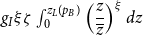
(20) \begin{equation} 1=\int _{\underline{z}}^{\overline{z}}\left (\frac{1}{g_{I}\zeta }\left (\frac{z}{\overline{z}}\right )^{\zeta }+1\right )f_{L} (z;\;\Theta )dz. \end{equation}

This is the condition which relates $\zeta$ and $g_{I}$ to the distribution parameters $\Theta$ . It is an equilibrium condition which consistently links the Left and Right distributions of profit income. Note that $\Theta$ can consist of multiple parameters (e.g. mean and standard deviation for log-normal distribution, right-truncated at $\overline{z}$ ).

2.4 Double-Pareto distribution

The exact shape of the left distribution $F_{L} (z;\;\Theta )$ depends on $\Phi (z;\;\Theta )$ , and hence the assumed function of $f_{H}(h;\;\Theta )$ . To fix our idea, let us consider

(21) \begin{equation} f_{H}(h )=\frac{\xi h^{\xi -1}}{\overline{h}^{\xi }},\qquad \xi \gt 1,\quad \underline{h}=0, \end{equation}

in what follows. This is a Pareto distribution of $h$ with $\Theta \equiv \left \{ \xi \right \}$ . We assume $\xi \gt 1$ to ensure that the density is strictly increasing. It is strictly concave for $1\lt \xi \lt 2$ , linear for $\xi =2$ and convex for $\xi \gt 2$ . Therefore, entrant entrepreneurs are more likely start with lower profit income as $\xi$ falls. In this sense, a lower $\xi$ exacerbates inequality in the left tail.Footnote ²⁰

Under this assumption, (20) is reduced to

(22) \begin{equation} \xi =\frac{1}{g_{I}}-\zeta . \end{equation}

This condition endogenously determines the value of $\xi$ for given $g_{I}$ and $\zeta$ such that flows of firms/entrepreneurs are consistent with the entire distribution of profit income. In particular, the Pareto exponents are negatively related, and its implications will be discussed below. Using (12) and (22), $\xi$ can be expressed in terms of Poisson rates of innovation

(23) \begin{equation} \xi =\frac{1-g_{E}}{g_{I}} \end{equation}

When (22) holds, $z$ is now distributed according to

(24) \begin{equation} F(z )=\begin{cases} F_{L}(z )=\dfrac{\zeta }{\xi +\zeta }\left (\dfrac{z}{\overline{z}}\right )^{\xi } & 0\lt z\leq \overline{z}\\ F_{L}(\overline{z} )+F_{R}(z )=1-\dfrac{\xi }{\xi +\zeta }\left (\dfrac{\overline{z}}{z}\right )^{\zeta } & \overline{z}\lt z\lt \infty \end{cases} \end{equation}

This is a double-Pareto distribution where $z$ exactly obeys the Pareto law in both tails.Footnote ²¹ Note that $F_{L}(\overline{z} )=g_{E}$ and $F_{R}(\infty )=1-g_{E}$ . This implies that the proportion $g_{E}$ of all entrepreneurs are located in the Left distribution and others are on the other side. The result is intuitive because a higher $g_{E}$ means that creative destruction occurs more often so that more firms tend be found in the Left distribution.

2.5 The number of monopoly industries

In this section, we consider the determination of $N$ which is the number of monopoly products in the economy. We derive it by examining the number of intermediate products flowing into and out of $N$ . The approach will be turn out to be useful for later analysis.Footnote ²²

When an entrepreneur succeeds in entrant innovation in industry $i$ , all incumbent products become obsolete in the industry and their number is $n_{i}g_{E}dt$ during time $dt$ . Integrating it over $i$ gives $\int _{0}^{i}n_{i}g_{E}dtdi=Ng_{E}dt$ which is the number of intermediate products flowing out of $N$ . On the other hand, an entrant creates $h$ number of products in $i$ . Given that $h$ is random, its average is

(25) \begin{equation} \int _{0}^{\overline{h}}hf_{H}(h )dh=\frac{\overline{h}\xi }{\xi +1}\equiv \hat{h}\left (\xi ;\;\overline{h}\right ). \end{equation}

Note that $\hat{h}\left (\xi ;\;\overline{h}\right )$ may include goods produced by the previous incumbent, and we count them as an inflow here. Therefore, $\hat{h}\left (\xi ;\;\overline{h}\right )g_{E}dt$ is an inflow of goods due to entrant innovation during $dt$ . In addition, new intermediate goods are created via incumbent R&D with an average flow of $n_{i}g_{I}dt$ products being generated during $dt$ in industry $i$ . Integrating it over $i$ gives $\int _{i\in \Xi _{i}}\left (n_{i}g_{I}dt\right )di=Ng_{I}$ .

Equating inflows and outflows gives

(26) \begin{align} Ng_{E}dt & =\left (\hat{h}g_{E}+Ng_{I}\right )dt \end{align}

(27) \begin{align} & \Downarrow \nonumber \\ N & =\frac{\overline{h}\xi \zeta }{\left (\xi +1\right )\left (\zeta -1\right )}\equiv N\left (\xi, \zeta ;\;\overline{h}\right ) \end{align}

A higher $\bar{h}$ raises $N$ because $\bar{h}$ determines the maximum number of monopoly products for entrant firms. To develop an intuitive explanation of how $\xi$ and $\zeta$ affect $N$ , recall that $N$ is equivalent to the average number of products produced by monopoly firms. Consider $\zeta$ which is negatively related to $N$ . A higher $\zeta$ , caused by a higher $g_{E}$ for a given $g_{I}$ (see (12)), means that a turnover of firms is relatively high, and hence the number of products per monopoly firm falls. On the other hand, $N$ rises as $\xi$ increases. (23) shows that a higher $\xi$ arises due to a lower $g_{E}$ for a given $g_{I}$ . It implies a lower turnover of firms, which is the opposite case of $\zeta$ . A finite value of $N$ requires $\zeta \gt 1$ .

3.1 iso-Gini contours

It is straightforward, though tedious, to show that the Gini coefficient of (24) is given by

(28) \begin{equation} G=\int _{0}^{\infty }F(z )(1-F(z ))=\frac{2\left (\xi ^{2}+\xi \zeta +\zeta ^{2}\right )+\xi -\zeta }{(2\xi +1)\left (\xi +\zeta \right )\left (2\zeta -1\right )}. \end{equation}

One can confirm that $G$ is decreasing both in $\xi$ and $\zeta$ . Fig. 5 draws an iso-Gini locus, which are convex to $\left (1,1\right )$ .Footnote ²³ Inequality measured by $G$ falls as we move northeastward. To interpret its slope, note that the Gini of the Right distribution would be $1/\left (2\zeta -1\right )$ if $F_{R}(z )$ alone was considered independently and calculated separately, and similarly $1/(2\xi +1)$ for $F_{L}(z )$ alone. This shows that a higher $\zeta$ and $\xi$ reduces the Gini within each side, and increasing $\zeta$ and reducing $\xi$ is akin to shifting inequality from the Right to the Left distribution. Following this interpretation, the slope of an iso-Gini curve is the marginal rate of substitution between inequalities in the Left and Right distributions. A unit increase $\zeta$ (falling inequality in the Right distribution) requires a fall in $\xi$ (increasing inequality in the Left distribution) by the amount equivalent to the slope of an iso-Gini curve for a given level of the Gini coefficient. A downward-sloping iso-Gini locus implies that a fall in either $\xi$ or $\zeta$ , taking the other Pareto exponent constant, necessarily increases the Gini coefficient.

Figure 5.

The four areas divided by iso- $S_{B}$ and iso- $S_{T}$ curves. Starting from $A0$ , the $X$ relationship holds in Areas 1 and 4.

3.2 Top/bottom income shares

The top/bottom income shares can also be easily calculated in our framework. For this, define $100\bar{p}$ with $\bar{p}=F\left (\bar{z}\right )$ as the percentile for $\bar{z}$ , the threshold income between the Left and Right distributions. First consider the bottom $100p_{B}$ % income share for $p_{B}\lt \bar{p}$ , which we use $S_{B}$ to denote. Appendix C shows that it is defined by

(29) \begin{equation} S_{B}=p_{B}^{1+\frac{1}{\xi }}\left (1-\frac{1}{\zeta }\right )\left (1+\frac{\xi }{\zeta }\right )^{\frac{1}{\xi }},\quad \text{for }p_{B}\leq \bar{p},\qquad \frac{\partial S_{B}}{\partial \xi }\gt 0,\quad \frac{\partial S_{B}}{\partial \zeta }\gt 0. \end{equation}

This equation allows us to draw an iso- $S_{B}$ curve in Fig. 5, which shows different combinations of $(\xi, \zeta )$ for a given $\left (S_{B},p_{B}\right )$ . $S_{B}$ increases in $\zeta$ because its higher value means a thiner right tails. $B_{B}$ is also increasing in $\xi$ despite that the left tail gets thiner with it. Its reason is more involved, but it is basically driven by the fact that net profit at the $100p_{B}$ percentile increases with a higher $\xi$ .Footnote ²⁴ The signs of the derivatives in (29) imply that, holding $p_{B}$ constant, $S_{B}$ gets higher/lower in the northeast/southwest area. This property will be exploited to examine how the income share changes in response to parameter changes.

In the appendix, we also derive the top $100(1-p_{T})\%$ income share (e.g. $1-p_{T}=0.01$ ), $S_{T}$ for $p_{T}\gt \bar{p}$ , which is defined byFootnote ²⁵

(30) \begin{equation} S_{T}=\left (1-p_{T}\right )^{1-\frac{1}{\zeta }}\frac{1+\dfrac{1}{\xi }}{\left (1+\dfrac{\zeta }{\xi }\right )^{\frac{1}{\zeta }}},\quad \text{for }p_{T}\geq \bar{p},\qquad \frac{\partial S_{T}}{\partial \xi }\lt 0,\quad \frac{\partial S_{T}}{\partial \zeta }\lt 0. \end{equation}

This defines an iso- $S_{T}$ locus in Fig. 5, giving different combinations of $(\xi, \zeta )$ for a given $\left (S_{T},1-p_{T}\right )$ . An intuition for the signs of the derivatives are similar to the one given for (29). The derivatives in (30) confirm that $S_{T}$ is larger/smaller in the southwest/northeast area for a constant $p_{T}$ .

Appendix C also demonstrates that an iso- $S_{T}$ curve is steeper than an iso- $S_{B}$ curve, giving rise to a unique intersection point $A0$ , as illustrated in Fig. 5. The two curves divide the $(\xi, \zeta )$ space into four areas. To interpret them, consider an economy located at $A0$ . The following list gives what happens as the economy moves from $A0$ to four regions, holding $p_{B}$ and $1-p_{T}$ constant:

1. Area 1: $S_{B}$ falls, and $S_{T}$ increases.

2. Area 2: $S_{B}$ increases, and $S_{T}$ increases (i.e. the income share of the middle income range between $p_{B}$ and $p_{T}$ falls).

3. Area 3: $S_{B}$ falls, and $S_{T}$ falls (i.e. the income share of the middle income range between $p_{B}$ and $p_{T}$ rises).

4. Area 4: $S_{B}$ increases, and $S_{T}$ falls.

Those four cases allow us to explore how income shares respond to parameter changes.

The next task is to locate an iso-Gini curve passing through $A0$ . Appendix D shows that if $p_{B}$ and $p_{T}$ are sufficiently different from $\bar{p}$ , an iso-Gini is steeper than an iso- $S_{B}$ curve, but less so than an iso- $S_{T}$ curve, as illustrated in Fig. 5. A word “sufficiently” does not mean $p_{B}\rightarrow 0$ or $p_{T}\rightarrow 1$ . In fact, an iso-Gini curve is sandwiched between those two iso-income share curves for a large range of values of $p_{B}$ and $p_{T}$ . For example, Toda (Reference Toda2012) obtains estimates of $\zeta =2.34$ and $\xi =1.15$ using US data from the Current Population Survey (2000–2009). He also shows that a calculated Gini coefficient based on those values is close to an actual value. Using the same numbers, we have $\bar{p}=0.67$ and the sandwiched case arises for $p_{B}\leq 0.65$ and $1-p_{T}\leq 1-0.67$ , which practically covers an almost entire range of values. In addition, our calibration analysis in the online appendix suggests that the sandwiched case is a norm.Footnote ²⁶

The $X$ inequality relationship between the Gini coefficient and the top/bottom income share in Table 1 corresponds to Areas 1 and 4 in Fig. 5. Now consider again an economy at $A0$ in the figure. Further suppose that the economy moves to a random point in $(\xi, \zeta )$ space. It is clear from the figure that the economy is more likely to end up in Areas 1 and 4 than other ares because the iso- $S_{B}$ and iso- $S_{T}$ curves are downward-sloping, that is the $X$ relationship is more likely to occur than otherwise. Having said this, however, the economy does not move randomly, but systematically according to economic incentives. To explore this, we need to endogenize R&D activity.

Figure 6.

Both panels use an income variable called “ptinc” (pre-tax national income; non-negative values only) with a frequency varaible “dweght” in Piketty et al. (Reference Piketty, Saez and Zucman2018).

3.3 Data and a double-Pareto approximation

In general, an observed income distribution does not follow a particular distribution, and different distributions are proposed to model it. Examples include exponential, lognormal, gamma, Levy-stable, double-Pareto-lognormal, and they are considered as an approximation of a true distribution at best.Footnote ²⁷ Similarly, we use a double-Pareto as an approximation of an underlying income distribution. But before we move on, we consider the extent to which the double-Pareto approximation is useful in understanding the $X$ inequality relationship. For this, we use data of Piketty et al. (Reference Piketty, Saez and Zucman2018). Its advantage is that it allows us to calculate summary statistics based on disaggregated data of 100% national income in the U.S.

We first examine some properties relevant to our analysis. Panel (a) of Fig. 6 shows a log-log plot of the data for five-year intervals in 1970–2015.Footnote ²⁸ The threshold is set to the 60th percentile and a tent map shape is clearly visible for all years.Footnote ²⁹ This visual inspection suggests that a double-Pareto distribution is in the ballpark.

Having said this, however, approximation means loss of information by definition (more on this later). In addition, a question remains on how to calculate the Left and Right tail Pareto exponents. A possibility may be to choose a given threshold percentile which divides the entire distribution into the Left and Right parts and calculate exponents, respectively. However, this approach does not necessarily generate the best fit. Instead, we search different percentiles to calculate $\hat{\xi }$ and $\hat{\zeta }$ separately and choose the ones which meet the following conditions: (i) $\hat{\xi }$ and $\hat{\zeta }$ are both greater than 1, and (ii) prediction errors measured by the coefficient of variation of root mean square deviation is minimized in five percentile intervals. According to these criteria, we found the 35th percentile as the upper threshold for the Left distribution and the 65th percentile as the lower threshold for the Right distribution in the 1981–2016 period. Panel (b) of Fig. 6 shows the maximum likelihood estimates of $\xi$ and $\zeta$ based on those percentiles. A clear downward trend is noticeable for $\hat{\zeta }$ . This means that the Gini coefficient tends to increase according to (28). On the other hand, $\hat{\xi }$ has a positive trend. This tends to decrease the Gini coefficient according to (28). An increasing trend of the Gini coefficient in the US means that the former effect dominates the latter.

Figure 7.

The plots labeled data are calculated using the same variables in Fig. 6. Those labeled double Pareto prediction use $\hat{\xi }$ and $\hat{\zeta }$ in Fig. 6 to calculate (28), (29), and (30).

Given those estimates, we compare the inequality indices calculated using data and predicted by a double-Pareto distribution with estimates of $\hat{\xi }$ and $\hat{\zeta }$ . Panel (a) of Fig. 7 shows the Gini coefficient. The predicted values closely follow the actual index, though slight deviation occurs in more recent years. As far as the Gini coefficient is concerned, a double-Pareto approximation works reasonably well.Footnote ³⁰ Panels (b) and (c) show the top 1% and 5% income shares. It is immediately clear that predicted values again closely move together with the data, though there are differences in levels. Level differences are even clearer for the bottom 30% and 40% income shares in Panels (d) and (e). They are due to information loss caused by a double-Pareto approximation. What is remarkable, however, is that the tendency of changes, that is the slope, is preserved for all of those indices. Indeed, the null hypothesis that the slopes of a linear trend of data and predicted values are the same cannot be rejected even at the 10% level for the Gini coefficient and the bottom 30% and 40% income shares. Regarding the top 1% and 5% income shares, although a similar null hypothesis can be rejected at 1% level, the figures suggest that the data and the approximated series move closely together. Because the purpose of our analysis is not to explain levels, but changes or trend of the inequality indices, we take a Double-Pareto distribution as a reasonable approximation of the underlying income distribution for our purposes.

4.1 Consumers

As mentioned above, consumers are risk-neutral, hence the interest rate $r$ is equal to the rate of time preferences. We assume that the price index associated with (1) is one.Footnote ³¹ Given these, the demand for $Y_{j}$ is

(31) \begin{equation} Y_{j}=\frac{E}{JP_{j}} \end{equation}

where $E$ is consumption expenditure and $P_{j}$ is the price of $Y_{j}$ .

4.2 Demand for intermediate products

Consumption goods $j$ is competitively produced according to (2). Profit maximization requires that $y_{ji}p_{ji}=Y_{j}P_{j}$ holds. Hence, a demand function of intermediate product $y_{ji}$ is given by

(32) \begin{equation} y_{ji}=\frac{E}{Jp_{ji}} \end{equation}

where $p_{ji}$ is the price of $y_{ji}$ .

4.3 Profits

One unit of intermediate goods is produced with one worker. Intermediate goods are produced competitively or by monopoly firms. In the latter case, like other Schumpeterian models, firms charge the price with the quality step $\lambda$ as a constant markup over the marginal cost, that is $p_{ji}=\lambda w$ where $w$ is wage. Therefore, profit per product is $\Lambda \dfrac{E}{J}$ where $\Lambda \equiv 1-\dfrac{1}{\lambda }$ .

4.4 R&D technology

To enter an intermediate good industry $i$ as a monopoly, an entrepreneur has to be successful in R&D first. Entrant innovation occurs with a Poisson arrival rate of $\overline{\delta }_{E}\equiv \dfrac{\delta _{E}}{R_{E}^{1-\mu }}$ for each entrepreneur. $R_{E}$ is the total number of entrepreneurs who engage in entrant R&D, and its presence in the denominator captures the negative congestion externality. Because of free entry, there are potentially many researchers, and each of them takes $R_{E}$ as given. The Poisson rate for the economy as a whole is $g_{E}=\overline{\delta }_{E}R_{E}$ or

(33) \begin{equation} g_{E}=\delta _{E}R_{E}^{\mu },\qquad \delta _{E}\gt 0,\quad 0\lt \mu \leq 1. \end{equation}

It is equivalent to $g_{E}$ in Section 2.

Recall that entrant R&D is undirected in the sense that an intermediate industry where innovation is implemented is randomly chosen from all industries $i\in [0,1 ]$ after innovation occurs. Once an industry $i$ is chosen, then all goods produced by the previous incumbent monopoly firm in $i$ , are rendered obsolete. Then, a range of goods with a measure $h_{i}\lt J$ is randomly selected for an entrant to start with, and their quality levels increases by a factor $\lambda$ . An entrepreneur earns profits $h_{i}\pi$ at the time of entry. Any other goods in $i$ are now competitively produced. $h_{i}$ goods may include those produced by the previous incumbent.

After entry, an entrepreneur in industry $i$ turns to incumbent R&D to increase profits further. If successful, a competitive product in $i$ is randomly picked and its quality rises by a factor $\lambda$ , increasing the entrepreneur’s profit by $\pi$ . We assume that incumbent R&D takes the form of multiple projects. A single project is financed out of profit arising from each intermediate goods production. That is, the number of R&D projects is equivalent to the number of products that firm produces. Specifically, innovation for each project follows a Poisson process with an arrival rate of

(34) \begin{equation} g_{Ii}=\delta _{I}R_{Ii}^{\gamma },\qquad \delta _{I}\gt 0,\quad 0\lt \gamma \lt 1 \end{equation}

where $R_{Ii}$ is the number of workers in each project of a firm in industry $i$ .

Now consider the expected change in $n_{i}$ due to incumbent R&D. Given multiple R&D projects, it changes according to

(35) \begin{equation} dn_{i}=1\times n_{i}g_{Ii}dt+0\times n_{i}\left (1-g_{Ii}dit\right )=n_{i}g_{Ii}dt. \end{equation}

Consider the first term of the first equality. A firm runs $n_{i}$ multiple projects, and each generates an arrival rate $g_{Ii}$ . Therefore, $n_{i}g_{Ii}dt$ is equivalent to a flow of innovations during $dt$ , each of which improves the quality of a good. The second term represents the case where projects fail. (35) shows that $n_{i}$ grows exponentially on average.

4.5 R&D decisions

Let us consider an R&D decision facing an incumbent firm with $n_{i}$ products. Let $V_{i}$ denote the value of the incumbent firm. Given (35), define the value of that firm:

(36) \begin{equation} V_{i}\left (n_{i}\right )=\max _{R_{Ii}}\left \{ n_{i}\pi _{i}dt+\mathbb{E}\left [\left (1-\rho dt\right )\left (1-g_{E}dt\right )V_{i}\left (n_{i}\left (t+dt\right )\right )+\left .V_{i}\left (t+dt\right )\right |_{n_{i}=\bar{n}_{i}}\right ]\right \} \end{equation}

where

(37) \begin{equation} \pi _{i}\equiv (1-\tau )\Lambda \frac{E}{J}-\left (1-s_{I}\right )wR_{Ii} \end{equation}

is after-tax profit net of R&D expenditure, $\tau$ is the corporate tax rate and $s_{I}$ is the rate of subsidy to incumbent R&D. The second term on the RHS of (36) is interpreted as follows. $V_{i}\left (n_{i}\left (t+dt\right )\right )$ is the value if an additional innovation occurs, and it is realized if no entrant innovation occurs with the probability of $(1-g_{E}dt)$ during $dt$ . The remaining term $(1-\rho dt)$ discounts the future value. The last term captures capital gains due to growth of $E$ and $w$ which is realized irrespective of innovation. Appendix F shows that the optimal $R_{Ii}$ is defined by

(38) \begin{equation} R_{Ii}=\left (\frac{\gamma \delta _{I}}{1-s_{I}}\cdot \frac{V}{w}\right )^{\frac{1}{1-\gamma }}\equiv R_{I}\quad \forall \;i\in [0,1 ] \end{equation}

where

(39) \begin{equation} V\equiv \frac{\pi }{\rho +g_{E}-g_{I}-g_{w}} \end{equation}

is the value of an incumbent firm per product or $V\equiv V_{i}\left (n_{i}\right )/n_{i}$ , and $g_{w}$ is the growth rate of wage which captures capital gains. The presence of $g_{E}$ in $V$ represents the risk of losing profits, and $g_{I}$ is an additional gain from incumbent innovation. Because R&D employment per product is the same for $i\in [0,1 ]$ (see (38)), we have

(40) \begin{equation} \pi _{i}=\pi, \qquad \quad g_{Ii}=g_{I} \end{equation}

They are equivalent to $\pi$ and $g_{I}$ in Section 2. $R_{I}$ in (38) is increasing in $\delta _{I}$ , $s_{I}$ and $V/w$ as expected.

Turning to entrant R&D decisions, recall that $h_{i}$ is a random variable, and so is the value of an entrant firm because it depends on $h_{i}$ . We therefore distinguish between its ex ante and ex post values. An ex ante or ex post value of innovation is the one before or after the result of uncertain R&D, that is the value of $h_{i}$ becomes known. In fact, the ex post value per product is equivalent to $V$ in (39), hence the ex post firm value is given by $h_{i}V$ . Next, let us use $v$ to denote the ex ante value of entrant innovation. Using the average of $h_{i}$ in (25), $v$ is given by

(41) \begin{equation} v=\hat{h}\left (\xi \right )V \end{equation}

because $V$ is the same for all intermediate good industries. Free entry is assumed, and it leads to

(42) \begin{equation} \frac{\delta _{E}}{R_{E}^{1-\mu }}v=\left (1-s_{E}\right )w \end{equation}

where $s_{E}$ is the rate of subsidy for entrant R&D.

To explore how R&D incentives respond to research-related parameters, let us use (38), (41) and (42) to get

(43) \begin{equation} \frac{R_{E}}{R_{I}}=\left [\frac{1-s_{I}}{1-s_{E}}\cdot \frac{\delta _{E}}{\delta _{I}}\cdot \frac{\hat{h}\left (\xi \right )}{\gamma }\right ]^{\frac{1}{1-\gamma }} \end{equation}

where we assume $\mu =\gamma$ , that is the extent of the diminishing returns of entrant and incumbent R&D is the same for simplicity. This assumption is maintained in what follows.Footnote ³² The ratio of entrant-to-incumbent R&D workers $R_{E}/R_{I}$ is increasing in $\left (1-s_{I}\right )\delta _{E}/\left (1-s_{E}\right )\delta _{I}$ . An intuition goes as follows. An increase in $\delta _{E}$ or $s_{E}$ encourages entrant R&D, but discourages incumbent innovations because the risk of losing all profits and existing the market rises. Regarding a higher $\delta _{I}$ or $s_{I}$ , it indeed promotes incumbent and entrant innovations because the value of a monopoly product $V$ increases. However, incumbent R&D incentives are larger than entrants’ to the extent that $R_{E}/R_{I}$ falls. (43) also shows that the relative R&D employment is increasing in $\hat{h}\left (\xi \right )$ , the average value of $h$ . This is because a higher $\hat{h}\left (\xi \right )$ raises the expected return from entrant R&D, leading to a greater employment in entrant R&D.

4.6 Labor market

There are four sources that require workers. First, the number of entrepreneurs earning profits is 1. This is because there is a single monopoly firm run by an entrepreneur in each of intermediate goods industry $i\in [0,1]$ . Second, workers are used for R&D. Those who engage in entrant R&D is $R_{E}=\left (g_{E}/\delta _{E}\right )^{\frac{1}{\gamma }}$ from (33). In addition, (22) and (23) allow us to write $g_{E}=\zeta /\left (\xi +\zeta \right )$ . Therefore, $R_{E}=\left \{ \zeta /\left [\delta _{E}\left (\xi +\zeta \right )\right ]\right \} ^{\frac{1}{\gamma }}\equiv R_{E}(\xi, \zeta )$ is equivalent to entrepreneurs trying to enter the intermediate goods industry. Incumbent R&D workers per product is similarly calculated from (34) and (22) as $R_{I}=\left (1/\delta _{I}\left (\xi +\zeta \right )\right )^{\frac{1}{\gamma }}\equiv R_{I}(\xi, \zeta )$ . The total number of workers used for incumbent research is $R_{I}N$ where $N$ is the number of monopoly firms, given in (27). The remaining workers are used for manufacturing, which employs $CZ/J+NZ/J\lambda =\left (J-\Lambda N\right )Z/J$ where $Z\equiv E/w$ . Workers are fully employed for

(44) \begin{equation} L=1+R_{E}(\xi, \zeta )+R_{I}(\xi, \zeta )N(\xi, \zeta )+\left [J-\Lambda N(\xi, \zeta )\right ]\frac{Z}{J} \end{equation}

5.1 Growth

Entrant and incumbent innovations improve quality of intermediate products. This manifests itself in the form of wage growth and utility growth.Footnote ³³ Indeed, Appendix E shows that the following holds in steady state

(45) \begin{equation} g_{Q}\equiv \frac{\dot{Q}}{Q}=\frac{\dot{w}}{w}=\frac{\dot{U}}{U} \end{equation}

where $\ln \left (Q\right )=\frac{1}{J}\int _{0}^{J}\int _{0}^{1}k_{ji}didj\cdot \ln \left (\lambda \right )$ and $Q$ is the overall quality index for the whole economy. Its changes during $dt$ are given by

\begin{equation*} d\ln \left (Q\right )=\frac {1}{J}\int _{0}^{J}\int _{0}^{1}\left (\begin {array}{l} \text {the number of quality}\\ \text {improvement during }dt \end {array}\right )\times \left [\left (k_{ji}+1\right )-k_{ji}\right ]didj\cdot \ln \left (\lambda \right ) \end{equation*}

Note that the number of innovations, entrant and incumbent, is equivalent to the right-hand side of (26). Therefore, we have

(46) \begin{align} g_{Q} & =(\overset{\begin{array}{l} \text{Entrant}\\ \text{Contribution} \end{array}}{\overbrace{g_{E}\hat{h}\left (\xi \right )}}+\overset{\begin{array}{l} \text{Incumbent}\\ \text{Contribution} \end{array}}{\overbrace{g_{I}N(\xi, \zeta )}})\ln \left (\lambda \right )=\frac{\zeta }{\xi +\zeta }N(\xi, \zeta )\ln \left (\lambda \right ) \end{align}

using (22), (12) and (27). The first equality decomposes growth into entrant and incumbent contributions. The former depends only on the Pareto exponent of the Left distribution $\xi$ because entrants start from there.

5.2 Equilibrium conditions

To solve the model, let us rewrite (43) as

(47) \begin{equation} \zeta =A\left (\frac{\xi }{\xi +1}\right )^{\frac{\gamma }{1-\gamma }},\qquad A\equiv \left (\frac{1-s_{I}}{1-s_{E}}\cdot \frac{\overline{h}}{\gamma }\right )^{\frac{\gamma }{1-\gamma }}\left (\frac{\delta _{E}}{\delta _{I}}\right )^{\frac{1}{1-\gamma }}. \end{equation}

We call it the R&D incentive condition. A positive relationship between $\zeta$ and $\xi$ captures the following mechanism of the optimal R&D decisions of entrant and incumbent firms. Note that $\zeta$ on the LHS captures the term $R_{E}/R_{I}$ of (43), which can be verified using (12), (33) and (34). Also note that $\xi /\left (\xi +1\right )$ on the RHS comes from $\hat{h}\left (\xi \right )$ which is the average number of products with which entrant firms start upon entry (see (25)). An increase in $\xi$ means a greater number of products for entrants and makes entrant R&D more attractive for potential entrepreneurs. In turn, this leads to a higher ratio of entrant-to-incumbent R&D workers $R_{E}/R_{I}$ , that is an increase in $\zeta$ .

The second condition is based on the ex ante value of successful entrant innovation. Rewriting the free entry condition (42) with (37), (39), (41), (44) and (46), one can derive what we call the ex ante firm-value condition:

(48) \begin{equation} \frac{\delta _{E}}{R_{E}(\xi, \zeta )^{1-\gamma }}v(\xi, \zeta )=1-s_{E} \end{equation}

where

(49) \begin{align} v(\xi, \zeta ) & \equiv \hat{h}\left (\xi \right )\frac{\Pi (\xi, \zeta )}{\Gamma (\xi, \zeta )} \end{align}

(50) \begin{align} \Pi (\xi, \zeta ) & \equiv (1-\tau )\Lambda \dfrac{L-1-R_{E}(\xi, \zeta )-R_{I}(\xi, \zeta )N(\xi, \zeta )}{J-\Lambda N(\xi, \zeta )}, \end{align}

(51) \begin{align} \Gamma (\xi, \zeta ) & \equiv \rho +\frac{\left (\zeta -1+\gamma \right )-\zeta N(\xi, \zeta )\left (\ln \lambda \right )}{\xi +\zeta }. \end{align}

Although (49), (50) and (51) look complicated, they have clear interpretations. $\Pi (\xi, \zeta )$ is the after-tax (gross) profit and $\Gamma (\xi, \zeta )$ is the effective discount rate, both expressed in terms of the two Pareto exponents.Footnote ³⁴ Therefore, $\Pi (\xi, \zeta )/\Gamma (\xi, \zeta )$ is the expected present value of a future steam of profits. Multiplied by $\hat{h}\left (\xi \right )$ , it gives the ex ante value of a successful R&D firm, denoted by $v(\xi, \zeta )$ .

Figure 8.

Steady state equilibrium as an intersection point between the R&D-incentive condition and the firm-value condition. Equilibrium is stable when the former is steeper than the latter. The line from the origin passing through the equilibrium point is equivalent to $(1-g_{E})/g_{E}$ . An iso- $g_{I}$ curve is defined by (22).

(47) and (48) is the system of two equations with two unknowns $(\xi, \zeta )$ . Note that $g_{E}$ and $g_{I}$ in equilibrium can be recovered once $\xi$ and $\zeta$ are determined, using (22) and (23). Before considering comparative statics, we distinguish two cases, focusing upon a unique equilibrium.Footnote ³⁵ The first case is illustrated in Fig. 8 where the R&D incentive condition is steeper than the ex ante firm-value condition at equilibrium.Footnote ³⁶ In the second case (not shown), the relative slopes are reversed. In what follows, we focus on the first case because its equilibrium is stable in the following sense. The R&D incentive condition is based on the optimal R&D decisions. Incumbents optimally chose $R_{I}$ , and $R_{E}$ is determined via free entry. In particular, when firms consider whether to conduct entrant R&D, they take the ex ante value, which is given by $v\equiv \hat{h}\left (\xi \right )V$ in (41), as given. In this sense, the R&D incentive condition (47) determines $\zeta$ , taking $\xi$ as given. On the other hand, the ex ante firm-value condition (48) essentially determines the Pareto exponent $\xi$ of the Left distribution where entrant firms start, taking $\zeta$ as given. Viewed this way, the case of equilibrium illustrated in Fig. 8 is stable. In addition, calibration analysis below shows that the stable case is a norm.

5.3 Comparative statics

Focusing on the stable case in Fig. 8, the following summarizes comparative statics results:

1. Result 1: Following an increase in $\lambda$ , $L$ or a fall in $J$ , $\rho$ , $\tau$ ,

• • $\xi$ and $\zeta$ decrease.

• • $g_{E}$ and $g_{I}$ increase.

• • the Gini coefficient increases, the bottom $p_{B}$ income share falls, and the top $p_{T}$ income share increases.

1. Result 2: Following an increase in $\delta _{I}$ or $s_{I}$ ,

• • $\xi$ and $\zeta$ decrease.

• • $g_{E}$ and $g_{I}$ increase.

• • the Gini coefficient increases, the bottom $p_{B}$ income share falls, and the top $p_{T}$ income share increases.

1. Result 3: Suppose that $\lambda$ is not too large such that $\Gamma (\xi, \zeta )-\rho \geq 0$ .

   Following an increase in $\delta _{E}$ or $s_{E}$ ,

• • $\xi$ decreases and $\zeta$ increases.

• • $g_{E}$ and $g_{I}$ change ambiguously.

• • changes in the Gini coefficient increases, the bottom $p_{B}$ income share falls, and the top $p_{T}$ income share are ambiguous.

1. Result 4: Suppose $s_{I}=s_{E}$ initially. Following a simultaneous increase in $s_{I}$ and $s_{E}$ ,

• • $\xi$ and $\zeta$ decrease.

• • $g_{E}$ and $g_{I}$ increase.

• • the Gini coefficient increases, the bottom $p_{B}$ income share falls, and the top $p_{T}$ income share increases.

To develop an intuition, note that $\xi /\zeta =\left (1-g_{E}\right )/g_{E}$ which is equivalent to the slope of a line from the origin to $A_{0}$ in Fig. 8. Also note that (22) defines an iso- $g_{I}$ contour with the slope of $-1$ . As we move southwestward in the figure, $g_{I}$ gets higher, and it becomes lower in the area above the iso- $g_{I}$ locus. Now, consider Result 1. A fall in $\tau$ , for example, means that an after-tax profit per product is larger. This effect manifests itself in a downward shift of the ex ante firm-value condition, moving an equilibrium from $A_{0}$ to $A_{1}$ . It causes the ratio $\xi /\zeta$ to fall, and $A_{1}$ is located below the iso- $g_{I}$ curve, given that the R&D-incentives condition unaffected. Intuitively, the tax reduction generates greater incentives for both types of R&D, but its impact on incumbent R&D is greater than entrant R&D because the effect is realized immediately for incumbents, but in future for entrants conditional on an R&D success. Such difference results in a fall in $\zeta \equiv g_{E}/g_{I}$ . The result also reveals the inequality-worsening effects of a lower corporate tax, and it is also empirically supported (e.g. see Nallareddy et al. (Reference Nallareddy, Rouen and Serrato2018)). Other parameters are similarly interpreted.

Turning to Result 2, as $\delta _{I}$ gets larger, the ex ante firm-value condition shifts down and the R&D incentive condition moves left. As a result, equilibrium moves from $A_{0}$ to $A_{2}$ . This is because a higher incumbent R&D productivity boosts an incentive for incumbent R&D. In fact, it also induces entrant R&D because a higher $\delta _{I}$ increases the ex ante value of entrant innovation. Those two effects reduce $\xi \equiv \left (1-g_{E}\right )/g_{I}$ . In addition, the effect on $g_{I}$ is strong to the extent that $\zeta \equiv g_{E}/g_{I}$ falls and inequality worsens for the same reason explained above. Regarding the subsidy rate of incumbent R&D $s_{I}$ , its higher value affects the R&D incentive condition only, moving equilibrium to $A_{3}$ in Fig. 8. $g_{E}$ is positively affected for the same reason as in a higher $\delta _{I}$ .

Result 3 summarizes the effects of entrant R&D productivity improvement and a higher rate of entrant subsidy. They affect the Pareto exponents differently, hence changes in the inequality indices are ambiguous. Intuitively, a greater $\delta _{E}$ or $s_{E}$ makes entrant R&D attractive, resulting in a higher $g_{E}$ . On the other hand, it increases the risk of losing profits for incumbent firms. This discourages incumbent R&D. Those effects lead to opposite changes in $\xi$ and $\zeta$ . The result adds to the explanation of the precursory studies about why firm entry can decrease or increase inequality. Jones and Kim (Reference Jones and Kim2018) show that entry of new firms tends to reduce inequality via creative destruction. On the other hand, entrants can increase inequality in Aghion et al. (Reference Aghion, Akcigit, Bergeaud, Blundell and Hémous2019) because of higher markups they enjoy. Aghion et al. (Reference Aghion, Akcigit, Bergeaud, Blundell and Hémous2019) also reported that entrant and incumbent innovations both are positively correlated with top 1% income share.

In Result 4, a simultaneous increase in the rate of subsidies to incumbent and entrant R&D is considered. The R&D-incentive condition is unaffected, while the ex ante firm-value condition shifts downward. A new equilibrium is given by a point like $A_{1}$ . It is the combination of the effects caused by a higher $s_{E}$ and $s_{I}$ in Results 2 and 3. This result qualitatively implies that more generous R&D subsidies may be behind the $X$ inequality relationship.

According to these results, most parameter changes, ceteris paribus, moves the economy to Areas 1 and 4 in Fig. 5. In this sense, our model predicts that those parameter shifts may have played a role in generating the $X$ inequality relationship. While these are useful insights, they do not inform us about the extent to which each factor contributed to the $X$ inequality relationship observed in many countries. To tackle this issue, we resort to calibration analysis in the online appendix.Footnote ³⁷

6.1 Step 1: calibrated values

Six parameters in Table 2 are externally set, including corporate profit tax rates and R&D subsidy rates which are borrowed from Akcigit and Ates (Reference Akcigit and Ates2023). The remaining parameters are internally set in the following way. Using data on the entry rate of establishments and the share of R&D workers along with the $\left (\hat{\xi },\hat{\zeta }\right )$ series in Panel (b) of Fig. 6, we set up the system of four equations to simultaneously determine the values of $\delta _{I}$ , $\delta _{E}$ , $\overline{h}$ and $\lambda$ over the 1981–2016 period for a given $J$ . Then, given these parameter values, we set $J=1.249$ to match the average annual TFP growth rate over the period. This gives us recalculated values of $\delta _{I}$ , $\delta _{E}$ , $\overline{h}$ and $\lambda$ .

Table 2.

Calibrated parameter values

A noticeable feature is that R&D productivity $\delta _{E}$ (for entrants) and $\delta _{I}$ (for incumbents) both steadily fell. Importantly, the rate of reduction in $\delta _{E}$ is 19.9% which is greater than 16.7% for incumbents. $\overline{h}$ is the maximum initial number of products for entrants, and it also fell by 16.2%. All these have important implications on the $X$ inequality relationship. Despite the parsimonious and stylized nature of the model, the Supplementary Material demonstrates that the fit of the model seems broadly reasonable.

6.2 Step 2: quantifying factors for the $\boldsymbol{{X}}$ inequality relationship

Note that the calibtrated values of $\delta _{E}$ , $\delta _{I}$ , $\overline{h}$ , $\lambda$ , $\tau$ , $s_{I}$ and $s_{E}$ change over the 1981–2016 period, being consistent with the model and, in particular, the Pareto exponents $\hat{\xi }$ and $\hat{\zeta }$ in Panel (b) of Fig. 6. Viewed this way, therefore, changes in the Gini coefficient, the top $p_{T}$ % income share and the bottom $p_{B}$ % income shares are the results of changing all parameters at the same time.

We quantify the contribution of each parameter to the $X$ relationship, following Akcigit and Ates (Reference Akcigit and Ates2023). We conduct counter-factual experiments by holding one parameter at the 1981 level at a time, while other parameters change as calibrated above. Inevitably, the inequality indices deviate from the original series, and such deviation allows us to measure the contribution of a parameter held fixed. We repeat this process for $\delta _{E}$ , $\delta _{I}$ , $\overline{h}$ , $\lambda$ , $\tau$ and $s_{I}=s_{E}$ . To quantify deviation, we use the following measure:

(52) \begin{equation} \Omega _{1}=\frac{D_{2016}-D_{2016}^{k}}{D_{2016}-D_{1981}} \end{equation}

$D$ refers to the Gini coefficient, the top 10% income share or the bottom 40% income share, and $k$ is a variable fixed at the 1981 level.Footnote ³⁸ For example, $D_{2016}$ is the Gini coefficient in 2016 and $D_{2016}^{k}$ is the Gini coefficient in 2016 with a variable $k$ is fixed at the 1981 level. $\Omega _{1}$ measures deviation in 2016. In the Supplementary Material, we also consider the average of deviation. Note that the larger the value of $\Omega _{1}$ , the greater the contribution made by a variable $k$ ( $\Omega _{1}$ can be is negative).

Figure 9.

Holding entrant R&D productivity $\delta _{E}$ fixed at the 1981 level.

Figure 9 shows the case of entrant R&D productivity $\delta _{E}$ . The Gini coefficient, the bottom 40% income share and the top 1% income share are shown, and series labeled “Double-Pareto Prediction” and “Data” are equivalent to those in Panels (a), (b) and (e) of Fig. 7. Series labeled “ $\delta _{E}$ fixed” show what would happen if the parameter was held constant at the 1981 level. Consider the left graph. For a constant $\delta _{E}$ , the Gini coefficient falls rather than rises. It means that a falling $\delta _{E}$ is so strong that if it is removed, then the Gini coefficient follows a clear negative trend. In this sense, a falling $\delta _{E}$ makes a significant contribution to an increase in the Gini coefficient. A similar pattern arises in the right graph of the top 1% income share, while a $\delta _{E}$ -fixed series is trend-less or has a slightly positive trend for the bottom 40% income share. Column (1) of Table 3 shows $\Omega _{1}$ values of such deviations. They are all positive, indicating the extent to which entrant R&D productivity $\delta _{E}$ contributes to raising the inequality indices.

Table 3.

Quantifying factors behind the $X$ inequality relationship

Results of other parameters are also reported in Table 3. It is worth mentioning that the values for $\delta _{I}$ are all negative. It means that a declinigng incumbent R&D productivity mitigated the worsening of inequality. Regarding other parameters, they show patterns similar to entrant R&D productivity $\delta _{E}$ , though their magnitude is smaller.

6.3 Declining business dynamism and Fiscal policy changes

A declining business dynamism is characterized by a falling pace of startups and new businesses with an increasing share of older firms. As Acemoglu et al. (Reference Acemoglu, Akcigit, Alp, Bloom and Kerr2018) argue, it would lead to adverse impacts on growth and productivity because it means a slower pace of reallocation of resources from less efficient to more efficient businesses. It is captured by a simultaneous fall in $\delta _{E}$ and $\overline{h}$ in our model. Indeed, their calibrated values show a clear negative trend (see Panel (c) and (c) of Figure 10 in the Supplementary Material).

To assess the contribution of a declining business dynamism to the $X$ inequality relationship, we fix those two parameters at the 1981 level and let others take their calibrated values. The results are shown in Column (7) of Table 3. The magnitude of the impacts are certainly large. However, compared with $\delta _{E}$ , an increase in the magnitude is not particularly dramatic. What it suggests is that $\delta _{E}$ and $\overline{h}$ have a relatively large “substitutability” in explaining the $X$ inequality relationship, especially for the bottom income share.

Akcigit and Ates (Reference Akcigit and Ates2023) argue that a declining business dynamism results from reduced knowledge diffusion between leading and lagging firms in technology, which may be caused by pro-incumbent fiscal policy changes, such as a substantial reduction of a statutory corporate tax rate and an increasing intervention in supporting R&D in the period. To examine the contribution of such fiscal policy changes to the $X$ inequality relationship, we hold $\tau$ and $s_{I}=s_{E}$ both fixed at the 1981 level, letting other parameters change. Column (8) of Table 3 reports their quantified effects. In fact, the magnitude increases nearly in a linear way in the sense that summing the numbers in (5) and (6) approximately gives the magnitude in Column (8). In this sense, those policy measures are “complimentary” and their changes appear to reinforce the effects of the other.

Given the above discussion, two results stand out. First, the effect of a declining business dynamism seems to have generated a large impact on the Gini coefficient. Second, Column (9) shows the ratio of (7) over (8). It indicates that the top income share is more affected directly by a declining business dynamism, and the bottom income share by the fiscal policy changes.