Introduction
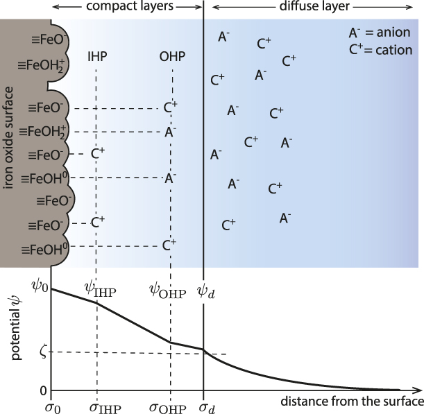
Metal oxide minerals are an abundant and reactive component of the Earth’s crust [Reference White1]. When oxides are immersed in aqueous solution, their surfaces acquire charge due to the ionization or dissociation of the surface oxo groups (i.e., protonation and deprotonation of surface exposed oxygen atoms) and preferential adsorption of ions [Reference Lyklema2, Reference Stumm and Morgan3, Reference Brown, Henrich, Casey, Clark, Eggleston, Felmy, Goodman, Grätzel, Maciel, McCarthy, Nealson, Sverjensky, Toney and Zachara4, Reference Brown5, Reference Brown and Calas6]. In electrolyte solutions, the surface excess charge is compensated by the layers of ions of opposite charge to the surface (counter-ions) and of similar charge (co-ions) [Reference Lyklema2, Reference Stumm and Morgan3, Reference Brown, Henrich, Casey, Clark, Eggleston, Felmy, Goodman, Grätzel, Maciel, McCarthy, Nealson, Sverjensky, Toney and Zachara4, Reference Brown5, Reference Brown and Calas6]. As a result, the equilibrium charge distribution at the interface, known as the electrical double layer (EDL), is established (Fig. 1) [Reference Lyklema2, Reference Stumm and Morgan3, Reference Brown, Henrich, Casey, Clark, Eggleston, Felmy, Goodman, Grätzel, Maciel, McCarthy, Nealson, Sverjensky, Toney and Zachara4, Reference Brown5, Reference Brown and Calas6]. The EDL strongly influences the reactivity of all hydrated oxide mineral surfaces, with impacts in environmental systems such as controlling pollutant remediation and element cycles in soils and groundwater. EDL models of the metal oxide/electrolyte interface consist of surface protonation reactions (e.g., 1-pK [Reference van Riemsdijk, de Wit, Koopal and Bolt10] and 2-pK [Reference Davis, James and Leckie11] models), the ion binding reactions, and the spatial distribution of counter-ions and co-ions charge. The thermodynamic descriptions of the EDL are based on models for the geometrical localization of the surface charge and electrolyte ions. The most detailed analytical descriptions of the EDL (e.g., the triple-layer model [Reference Davis, James and Leckie11, Reference Yates, Levine and Healy12]) divide the interface structure into layers that neglect lateral heterogeneity [Reference Lyklema2, Reference Stumm and Morgan3, Reference Brown, Henrich, Casey, Clark, Eggleston, Felmy, Goodman, Grätzel, Maciel, McCarthy, Nealson, Sverjensky, Toney and Zachara4, Reference Brown5, Reference Brown and Calas6]. Moreover, water is modeled as a structureless, inert medium with a dielectric constant between 4 and 10 [Reference Stumm and Morgan3, Reference Björneholm, Hansen, Hodgson, Liu, Limmer, Michaelides, Pedevilla, Rossmeisl, Shen, Tocci, Tyrode, Walz, Werner and Bluhm13]. The value of ε is most frequently approximated as 6 because it corresponds to the hypothetical situation of dielectrically saturated water in which all water dipoles are aligned with the electric field and act as though they are not associated (i.e., not hydrogen-bonded) [Reference Bockris and Khan14]. This extreme regime corresponds to the dielectric constant of water at high frequency (ε∞ = 5.2–6.0) [Reference Raicu and Feldman15].
Illustration of the EDL model (four-layer model) of iron oxide/electrolyte interface [Reference Bousse and Meindl7, Reference Bowden, Nagarajah, Barrow, Posner and Quirk8, Reference Charmas, Piasecki and Rudzinski9]. The surface potential (ψ0) is due to the protonation/deprotonation of the surface exposed FeOH groups; the electrokinetic potential (ζ) is formed at the shear plane of the EDL (i.e., near the boundary between the rigid and diffuse part of the EDL). The compact layer of the specifically adsorbed counter- and co-ions is referred to as inner Helmholtz plane (IHP) and the electrostatically bound counter- and co-ions as the outer Helmholtz plane (OHP). The diffuse part of the EDL is described by the Gouy–Chapman theory.

Experimental studies [Reference Toney, Howard, Richer, Borges, Gordon, Melroy, Wiesler, Yee and Sorensen16, Reference Shen and Ostroverkhov17, Reference Henderson18, Reference Carrasco, Hodgson and Michaelides19, Reference Fenter and Sturchio20, Reference Israelachvili and Pashley21] and molecular simulations [Reference Spohr22, Reference Wieckowski23, Reference Wang, Kalinichev and Kirkpatrick24, Reference Lee and Rossky25, Reference Philpott and Glosli26, Reference Zarzycki, Kerisit and Rosso27, Reference Zarzycki and Rosso28, Reference Zarzycki, Kerisit and Rosso29] of the hydrated interface offer an entirely different view of the properties and roles of water in the EDL: interfacial water is highly structured and the structured water layers generate a polarization potential capable of screening effectively the surface potential. For instance, molecular dynamics (MD) simulations showed that the electrostatic potential at the AgCl/KCl electrolyte interface due to water orientation is larger than the potential arising due to the electrolyte ion distribution [Reference Zarzycki and Rosso28, Reference Zarzycki, Kerisit and Rosso29]. This is in striking contrast to the analytical electrochemical calculations in which water structure is considered as structureless continuum that only changes the strength of the electrostatic interactions by lowering the dielectric constant at the surface (ε is supposed to be restored to its bulk value at distances >6 Å from the electrode surface) [Reference Bockris and Khan14].
To date, there is lack of a complete understanding of the extent of interfacial water structure formation and the consequences for metal oxide surface processes that occur within the EDL. MD simulations predict that interfacial water layering causes significant energy barriers for ion adsorption and formation of outer- and inner-sphere complexes [e.g., Fe(II) at goethite, α-FeOOH] [Reference Zarzycki, Kerisit and Rosso29, Reference Zarzycki and Rosso30]. However, the development of interfacial polarization potentials has not been included in any EDL models of the oxide/electrolyte interface. Recently, we developed a constant pH molecular dynamics (cpHMD) [Reference Mongan, Case and McCammon31, Reference Zarzycki, Smith and Rosso32] method incorporating surface charge constraints [Reference Zarzycki and Rosso30] that is capable of simulating oxide surface protonation/deprotonation processes, and associated solution dynamics, over timescales inaccessible to conventional MD. Here, we describe a simulation method designed to obtain further insight into the coupling between water ordering and a resulting polarization potential at vicinal surfaces exposed by a goethite nanoparticle (α-FeOOH). Our simulation results have important new implications for a wide range of chemical and physical processes controlled by the structure and dynamics at metal oxide/water interfaces, including particle aggregation and oriented attachment, precipitation–dissolution, mineral recrystallization, and coupled reactivity of confined hydrated surfaces.
Theory and implementation
There are numerous molecular simulation studies of charged metal oxide/electrolyte interfaces, but there are very few that implicitly considered the pH-dependent surface charge dynamics [Reference Borkovec33, Reference Borkovec, Daicic and Koper34, Reference Rustad, Wasserman, Felmy and Wilke35, Reference Zarzycki36, Reference Zarzycki37, Reference Zarzycki and Rosso38, Reference Zarzycki, Chatman, Preočanin and Rosso39, Reference Rustad and Felmy40]. Most of the reported molecular modeling studies were carried out using the charge neutral surfaces and therefore describe the surfaces at the pH corresponding to the point of zero charge (PZC). One of the first approaches to actually model proton release and binding to the metal oxide surfaces and to computationally validate the surface protonation models (e.g., 1-pK) was introduced by Borkovec et al. [Reference Borkovec33, Reference Borkovec, Daicic and Koper34]. Inspired by these papers, a similar stochastic simulation model was implemented, which also includes surface heterogeneity effects, electrolyte ion binding, and correlation [Reference Zarzycki36, Reference Zarzycki37, Reference Zarzycki and Rosso38, Reference Zarzycki, Chatman, Preočanin and Rosso39, Reference Zarzycki41, Reference Zarzycki42, Reference Zarzycki43, Reference Zarzycki, Charmas and Szabelski44, Reference Szabelski, Zarzycki and Charmas45]. These early simulation models, however, considered water only implicitly (as a dielectric continuum) and reduced the actual metal oxide surfaces to the lattice composed of the protonatable surface sites (i.e., as a discrete charge Ising model) [Reference Borkovec33, Reference Borkovec, Daicic and Koper34, Reference Zarzycki36, Reference Zarzycki37, Reference Zarzycki and Rosso38, Reference Zarzycki, Chatman, Preočanin and Rosso39, Reference Zarzycki41, Reference Zarzycki42, Reference Zarzycki43, Reference Zarzycki, Charmas and Szabelski44, Reference Szabelski, Zarzycki and Charmas45]. The first fully-atomistic simulations of the charged metal oxide/electrolyte interface with pH-dependent surface charge and the explicit water models were carried out by Rustad et al. [Reference Rustad, Wasserman, Felmy and Wilke35, Reference Rustad and Felmy40]. Here, the simulation results obtained by using the cpHMD algorithm are presented. The cpHMD methodology has been developed originally for the biological systems [Reference Mongan, Case and McCammon31], but recently, it was also adopted for the goethite/electrolyte interface [Reference Zarzycki, Smith and Rosso32].
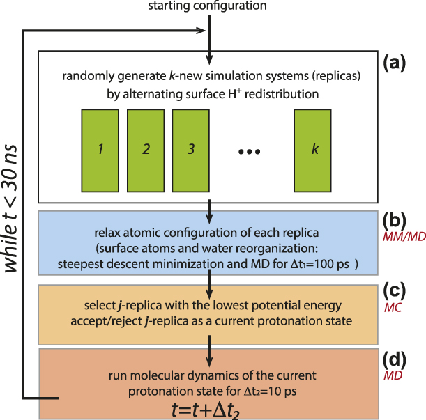
The cpHMD algorithm alternates Monte Carlo (MC) sampling of the accessible protonation configurations and MD simulations of the response to altered charge distributions [Reference Mongan, Case and McCammon31, Reference Zarzycki, Smith and Rosso32]. As described, in more detail, elsewhere [Reference Zarzycki and Rosso30, Reference Zarzycki, Smith and Rosso32], we use the replica-exchange approach to model dynamic proton redistribution. From a given protonation state i, our code generates a number of new protonation states (replicas) by swapping H+ between surface hydroxyl groups with the constraint that the total surface charge of a given crystal face remains unchanged. This constraint allows the dynamic redistribution of H+ ions on a given crystal face but does not allow them to move from one crystal face to another. The atomic configuration of each new protonation replica is subsequently optimized (using steepest descent energy minimization) and the solvent is allowed to reorganize for 100 ps using the MD simulation routine. Among all replicas, our simulation algorithm selected the lowest energy one as a candidate for the new protonation state j, which is accepted either if it has a lower energy than the current H+ proton redistribution i or if it satisfies the Metropolis–Hastings acceptance function:
 $$P\left( {i \to j} \right) = \min \left( {1,\exp \left( { - {{\Delta U} \over {{k_{\rm{B}}}T}}} \right)} \right)\quad ,$$
where ΔU = ΔU vdw + ΔU elec is the potential energy difference between j and i protonation states.
In the MC and MD steps, the long-range electrostatic energy was calculated using the classical Ewald summation scheme, in which the electrostatic energy U elec is given by the following equation [Reference Frenkel and Smit46]:
 $$4\pi {\varepsilon _0}{U^{{\rm{elec}}}} = {{2\pi } \over V}\sum\limits_{\vec{k} \ne 0} {{{{{\left| {S\left( {\vec{k}} \right)} \right|}^2}} \over {{k^2}}}{{\rm{e}}^{ - {{{k^2}} \over {4\alpha }}}}} + {1 \over 2}\sum\limits_{n \ne m}^N {{{{q_n}{q_m}} \over {{r_{nm}}}}{\rm{erfc}}\left( {{r_{nm}}\sqrt \alpha } \right)} - \sqrt {{\alpha \over \pi }} \sum\limits_n^N {q_n^2} \quad ,$$
where n and m are run-over ion indexes, N is the total number of charged ions in the system, V is the cell volume,  $\vec{k}$ is a vector in the reciprocal (Fourier) space, r nm is the distance between the ions n and m, and erfc is the complementary error function (i.e.,
 ${2 \over {\sqrt \pi }}\int_{{r_{nm}}\sqrt \alpha }^\infty {{{\rm{e}}^{ - {x^2}}}{\rm{d}}x}$). The term
 $S\left( {\vec{k}} \right)$ is the charge structure factor and describes the Gaussian-smeared charge density in the reciprocal space [i.e.,
 $\sum\limits_n^N {{q_n}\exp \left( {i\vec{k} \cdot {{\vec{r}}_n}} \right)}$], i is the imaginary unit].
The electrostatic contribution to forces acting on an ion n is obtained by differentiation of U elect with respect to r n (i.e.,  ${\vec{f}_n} = - {{{\rm{d}}U} \over {{d_{{{\vec{r}}_n}}}}}$):
 $$- 4\pi {\varepsilon _0}\vec{f}_n^{{\rm{elec}}} = {{{q_n}i\pi } \over V}\sum\limits_{\vec{k} \ne 0} {{{\vec{k}\left( {S\left( {\vec{k}} \right)} \right)} \over {{k^2}}}{{\rm{e}}^{i\vec{k} \cdot {{\vec{r}}_n} - {{{k^2}} \over {4\alpha }}}}} - {q_n}\sum\limits_{m \ne n}^N {{{{q_m}} \over {{r_{nm}}}}\left( {{{{\rm{erfc}}\left( {{r_{nm}}\sqrt \alpha } \right)} \over {{r_{nm}}}} + 2\sqrt {{\alpha \over \pi }} {{\rm{e}}^{ - \alpha r_{nm}^2}}} \right){{{{\vec{r}}_{nm}}} \over {{r_{nm}}}}} \quad ,$$
which is derived using  ${{{\rm{derfc}}\left( {{r_n}\sqrt \alpha } \right)} \over {{\rm{d}}{r_n}}} = - 2{{\rm{e}}^{ - \alpha r_n^2}}\sqrt {{\alpha \over \pi }}$ and
 ${{{\rm{d}}{{\left| {S\left( {\vec{k}} \right)} \right|}^2}} \over {{\rm{d}}{r_n}}} = 2{q_n}i\vec{k}{{\rm{e}}^{i\vec{k}{r_n}}}S\left( {\vec{k}} \right)$. The cutoff distance (10 Å) was applied for the short-range interactions and the real part of the Ewald sum. Equation (11) is used in calculating forces in MD part of the cpHMD algorithm. The time evolution of the system in the MD part is obtained by using the three-step velocity Verlet algorithm [Reference Swope, Andersen, Berens and Wilson47]:
 $$\overrightarrow {{r_i}} \left( {t + \delta t} \right) = \overrightarrow {{r_i}} \left( t \right) + \overrightarrow {{v_i}} \left( t \right)\delta t + {1 \over 2}{\left( {\delta t} \right)^2}\left( {{{\overrightarrow {{F_i}} \left( t \right)} / {{m_i}}}} \right)\quad ,$$
 $$\overrightarrow {{v_i}} \left( {t + {1 \over 2}\delta t} \right) = \overrightarrow {{v_i}} \left( t \right) + {1 \over 2}\delta t\left( {{{\overrightarrow {{F_i}} \left( t \right)} / {{m_i}}}} \right)\quad ,$$
 $$\overrightarrow {{v_i}} \left( {t + \delta t} \right) = \overrightarrow {{v_i}} \left( {t + {1 \over 2}\delta t} \right) + {1 \over 2}\delta t\left( {{{\overrightarrow {{F_i}} \left( {t + \delta t} \right)} / {{m_i}}}} \right)\quad ,$$
where  $\overrightarrow {{r_i}}$ and
 $\overrightarrow {{v_i}}$ are the i-atom position and velocity vectors, δt is the time step, and
 ${{\overrightarrow {{F_i}} } / {{m_i}}}$ is the acceleration of atom i. The rigid structure of the water molecule was preserved using the two-step RATTLE algorithm with the effective force
 $\overrightarrow {{F_i}} \left( t \right)$ in Eqs. (4)–(6) corrected by the bond-constraining force if atom i is bonded to any other atom [Reference Andersen48].
MD simulations for a newly accepted protonation state were carried out for another 10 ps with a time step dt = 1 fs before attempting to change the protonation state by using the MC scheme [Reference Zarzycki and Rosso30]. A new protonation state used further in MD is the lowest energy replica among several generated from the current protonation state in parallel MC runs. The simulation algorithm is illustrated in Fig. 2.
Diagram of the cpHMD algorithm: (a) generate a number of trial protonation states (replicas), (b) relax energy of each replica using MD, (c) the lowest energy relaxed protonation state is selected with weight given by Metropolis function for (d) the further system evolution.

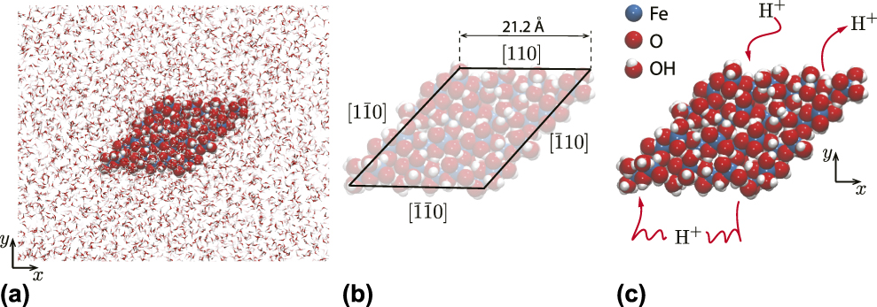
The goethite nanoparticle used in this study and the force–field parameters are identical to those reported in our previous studies [Reference Zarzycki and Rosso30, Reference Zarzycki, Smith and Rosso32], and inspired by related Fe(II)-catalyzed goethite recrystallization experiments (Fig. 3) [Reference Handler, Frierdich, Johnson, Rosso, Beard, Wang, Latta, Neumann, Pasakarnis, Premaratne and Scherer49]. The particle exposes dominant {110} (in Pbnm space group) prismatic face terminations typical of needle-shaped crystallites. The charge-neutral particle is generated by protonating active surface oxygen sites in accordance with their expected proton affinities [Reference Venema, Hiemstra, Weidler and van Riemsdijk50], with immersion in Simple Point Charge/Extended model (SPC/E) water and relaxation using the steepest descent algorithm. The subsequent temperature and density optimization steps were carried out using the NVT (canonical, constant number of particles N, volume V, and temperature T) and NPT (isothermal-isobaric, constant number of particles N, pressure P and temperature T) ensembles (T = 298 K, P = 1 atm., the Langevin thermostat with a collision frequency γ = 2 ps−1, and the Berendsen thermostat–barostat) [Reference Zarzycki and Rosso30]. The cpHMD simulations were carried out for 30 ns and the configurations were saved every 0.1 ps. The parallelization was provided by the message passing interface [Reference Walker and Dongarra51, Reference Gropp, Lusk, Doss and Skjellum52] library, and it allows to run the simulation in parallel using 4 nodes, each with 16 CPU cores (3.1 GHz Intel Xeon E52687W). The major performance bottlenecks were the Ewald summation procedure and writing simulation trajectory to the hard drive. A single cpHMD simulation run of 30 ns took around 9 days.
Illustrations of the simulation system. (a) The goethite (α-FeOOH) nanoparticle immersed in water. (b) Dimensions of the goethite nanoparticle. Each face is crystallographically equivalent. (c) H+ ions populate surface sites at a density consistent with an assumed solution pH. Protons on each face redistribute according to the MC algorithm but are constrained to a single given face, enabling a pH difference to be imposed in some simulations.

In order to simulate the interface structure at a given solution pH, protons are added or removed from surface sites to achieve a surface charge density consistent with experimentally determined titration curves [Reference Zarzycki and Rosso30].
Here, we study the effect of a surface charge imbalance between separated, crystallographically equivalent faces. Protons are transferred between opposite faces to achieve a protonation imbalance (ΔH +) and then allowed to redistribute among sites on a single face but not to migrate between faces. Although this condition is not achievable in experimental systems, it provides a simple approach for studying lateral communication of water structure between mineral particle faces. Here, we report the simulation results of a goethite particle in the bulk water without any explicit electrolyte ions to isolate the effect of the water polarization potential. We will present the more complex simulation scenarios with a fully developed EDL of varying thickness in the future.
The most relevant analysis for this study is the calculation of surface electrostatic properties, which are defined via the Poisson’s equation:
 $${\nabla ^2}\psi = - {\rho \over {{\varepsilon _0}}} = - \nabla \cdot E\quad ,$$
where ψ is the electrostatic potential, ρ is the charge density, E is the electrostatic field, ε0 is the static dielectric constant, and ∇ and ∇2 are divergence and divergence of a gradient (Laplacian) operators, respectively.
The y-axis projections of the charge density, ρ(y), and the electrostatic potential, ψ(y), are obtained as follows [Reference Spohr22, Reference Wieckowski23, Reference Wang, Kalinichev and Kirkpatrick24, Reference Lee and Rossky25, Reference Philpott and Glosli26, Reference Zarzycki, Kerisit and Rosso27, Reference Zarzycki and Rosso28, Reference Zarzycki, Kerisit and Rosso29, Reference Zarzycki and Rosso30]:
 $$\rho \left( y \right) = \sum\limits_{j = 1}^N {e{q_j}\delta \left( {{y_j} - y} \right)} ,\quad \langle \rho \left( y \right)\rangle = {1 \over {{N_{\rm{f}}}}}\sum\limits_{i = 1}^{{N_{\rm{f}}}} {\rho \left( y \right)} \quad ,$$
 $$\psi \left( y \right) = - {1 \over {{\varepsilon _0}}}\int {{\rm{d}}y} \int {\langle \rho \left( y \right)} \rangle {\rm{d}}y\quad ,$$
where δ is the Dirac delta function, e is the elementary charge, q j is the charge on j-atom, ε0 is the vacuum permittivity, and ρ(y) is the time-averaged charge density profile (averaged over all trajectory frames, N f). The two-dimensional charge density profile (projected on the x, y plane) is given by the following equation:
 $$\langle \rho \left( {x,y} \right)\rangle = {1 \over {{N_{\rm{f}}}}}\sum\limits_{i = 1}^{{N_{\rm{f}}}} {\sum\limits_{j = 1}^N {e{q_j}\delta \left( {{y_j} - y} \right)\delta \left( {{x_j} - x} \right)} } \quad .$$
Finally, the net difference in the charge density between two simulation runs (i, j) that differ in the proton imbalance between the mirrored [110] and  $\left[ {\bar{1}\bar{1}0} \right]$ faces, is given by the following equation:
 $$\Delta \langle \rho \left( {x,y} \right)\rangle = {\langle \rho \left( {x,y} \right)\rangle _i} - {\langle \rho \left( {x,y} \right)\rangle _j}\quad .$$
The electrostatic properties and atomic densities calculated in this study are the time-averaged properties of the system that reflects the time-dependent evolution of all atoms and stochastic evolution of the protonation states.
Results
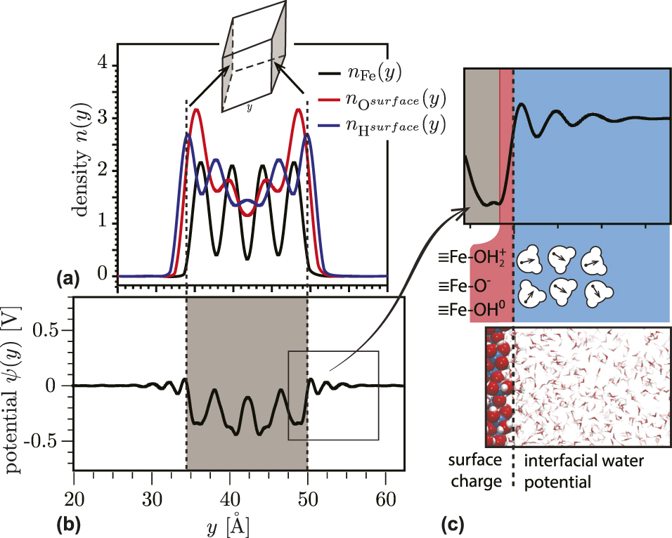
We first summarize the water ordering on a charge-neutral, proton-balanced goethite particle. The overall charge on the nanoparticle is neutral, corresponding to a solution pH equals to the PZC (pHPZC ∼ 9.1) [Reference Zarzycki and Rosso30]. There is no potential difference imposed between equivalent faces, so ΔH + = 0. In Fig. 4(a), the atomic densities and electrostatic potential are projected on the y-axis. The particle surface is defined by the peaks of surface protons [Figs. 4(a) and 4(b)]. The calculated electrostatic potential profile along the y-axis [Eq. (9)] shows near-surface modulation due to the layering of interfacial water [Figs. 4(b) and 4(c)]. The ordering decays with distance from the surface in an oscillating fashion, with a period corresponding to a typical water–water distance (3.1–3.2 Å). The predicted layering effect disappears at distances above ∼15 Å for both the neutral [Figs. 4(b) and 4(c)] and charged surfaces. Water layer development has been observed in prior simulations [Reference Spohr22, Reference Wieckowski23, Reference Wang, Kalinichev and Kirkpatrick24, Reference Lee and Rossky25, Reference Philpott and Glosli26, Reference Zarzycki, Kerisit and Rosso27, Reference Zarzycki and Rosso28, Reference Zarzycki, Kerisit and Rosso29], but the present cpHMD simulation shows that the time-averaged structure develops even when surface protons are allowed redistribute dynamically as expected for natural interfaces.
(a) Atomic density and (b, c) electrostatic potential profiles along the y-direction of particle with the charge-neutral surfaces. The water orientational response to the surface charge and interfacial layering results in the modulation of the electrostatic potential as a function of distance from the particle surface (b, c).

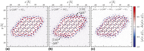
In Fig. 5(a), the water charge density is averaged over the z-direction onto the xy-plane [Eq. (10)]. The charge maps were obtained from 30-ns simulation trajectories that were re-centered on the goethite particle. The negative charge (blue) corresponds to water oxygen atoms and the positive charge (red) corresponds to water hydrogen atoms. The semispherical shapes of the charge density spots in the first three water layers, as seen previously in conventional MD studies [Reference Spagnoli, Gilbert, Waychunas and Banfield53], are a manifestation of the limited rotational and translational mobilities of the interfacial water. Although the goethite surfaces have no net charge, they impart net polarization to the interfacial water. The charge density layers appear to be packed more densely at the particle edges than at the mid-surfaces. This is in good agreement with the predictions of a fully dissociable water model [Reference Rustad and Felmy40]. In each case, the edge atoms that are more water solvated exhibit higher proton affinity. As expected for the proton-balanced simulation, there are no differences in the polarization charge distribution on the equivalent faces.
Maps of the time-averaged charge density of water molecules 〈ρ(x, y)〉 around a single goethite nanoparticle in water in μC/nm3. (a) A charge-neutral, proton-balanced particle with all faces equivalent. (b) A charge-neutral, proton-imbalanced particle. The (110) face is positively charged (ΔH + = +50), whereas the  $\left( {\bar{1}\bar{1}0} \right)$ face is negatively charged (ΔH + = −50). (c) Map of the difference in the time-averaged charge densities displayed in (a) and (b) (converted to e/nm3 to preserve the color scale).

To study the lateral propagation of water structure, we simulated a net charge-neutral but proton-imbalanced goethite nanoparticle, in which protons were transferred between two mirrored faces. Figure 5(b) displays the surface charge densities for a proton imbalance of ΔH + = 50 applied to the top and bottom surfaces, corresponding to an equivalent solution pH of ∼2.7 and ∼13.4, respectively. The difference in the surface charge of our particle is much larger than expected in the actual system to more clearly observe the long-range correlation in the interfacial water polarization, but it represents the actual interactions between two adjacent surfaces. A visual comparison shows that the predicted structure of the polarized interface differs for ΔH + = 0 [Fig. 5(a)] and ΔH + = 50 [Fig. 5(b)]. For visual clarity, in Fig. 5(c), we plotted the charge density difference between the proton-balanced and the proton-imbalanced nanoparticles. If the water structure on each face is affected only by the net charge density, on that face we would expect that the difference maps for the bystander faces will be close to zero. Instead, the charge density difference maps reveal that water structure on all six faces is highly sensitive to protonation changes made at only two of the faces.
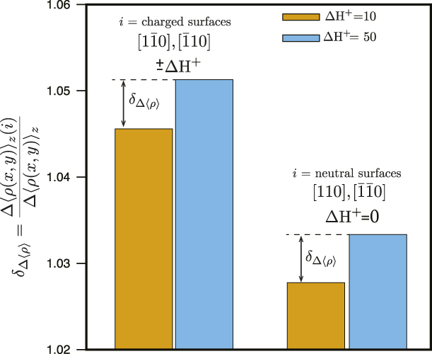
In Fig. 6, we provide simulation-averaged quantification of the effect by integrating the relative change in the net water polarization charge density [i.e., Fig. 5(c)] at the charged surfaces (ΔH + = 50) and vicinal surfaces, where ΔH + = 0. When two mirrored surfaces become charged, we observe a significant change in the water polarization on those surfaces compared with the case, in which the goethite nanoparticle has only net neutral surfaces (left columns in Fig. 6). We further observe that the unaltered surfaces also exhibit an increase in water polarization (right columns in Fig. 6). For all surfaces, the effect increases with increasing charge imbalance. The present study is limited to a single-geometry goethite nanoparticle with ∼21 Å dimensions, and more work will be required to determine the distance over which water polarization can propagate laterally. Nevertheless, as discussed below, this phenomenon is relevant to a range of processes, such as particle-oriented aggregation, dissolution, precipitation, and interfacial reactivity.
Histograms showing the relative differences in the integrated water polarization charge density between surface pairs. The left columns show the relative difference between charged surfaces for two values of the imposed charge: ΔH + = 50 [Fig. 5(c)] and ΔH + = 10 (an additional simulation not shown). The right columns show the relative differences in water polarization charge density between the pair of neutral surfaces.

Discussion
The present study is to our knowledge the first demonstration that the structure of interfacial water on an oxide mineral termination face is not independent of the water structure on neighboring faces. Rather, lateral hydrogen bond networks propagating from a highly charged face with polarized water molecules can strongly influence the order on neighboring faces. The actual particle will have a lower potential gradient and less pronounced polarization of interfacial water than shown in our simulations, but the same type of interactions between two adjacent surfaces will be present. This work demonstrates that the development of a polarized interface affects the time-averaged orientation of water at least three molecular distances away in both the perpendicular and lateral directions. This is an important finding, because it shows that the water structuring at the interface is due to a competition between the water propensity to preserve a tetrahedral hydrogen bond network and to align with the electric field generated by the charged surface. This prediction is consistent with recent experimental and simulation studies that have provided an increasingly detailed three-dimensional depiction of the molecular structure of EDLs in aqueous systems and macromolecular systems, including ionic liquids [Reference Liu, Zhang, Wu and Hu57, Reference Tamam, Ocko, Reichert and Deutsch58, Reference Merlet, Limmer, Salanne, van Roij, Madden, Chandler and Rotenberg59, Reference Kornyshev and Qiao60].
It remains a challenge to incorporate nanoscale and molecular scale phenomena into computationally tractable analytical models of EDL properties. Recent contributions have described modified EDL models incorporating interface roughness [Reference Zarzycki41, Reference Zarzycki42, Reference Zarzycki43, Reference Zarzycki, Charmas and Szabelski44, Reference Szabelski, Zarzycki and Charmas45, Reference Valtiner, Banquy, Kristiansen, Greene and Israelachvili61] or finite ion correlations [Reference Zarzycki42, Reference Voukadinova, Valiskó and Gillespie62, Reference Jiménez-Ángeles and Lozada-Cassou63, Reference Forsman64, Reference Sushko and Rosso65, Reference Shen, Chun, Rosso and Mundy66]. In principle, classical EDL models could incorporate both vertical and lateral water polarization phenomena if the Poisson’s equation [Eq. (7)] is solved in all three dimensions, that is:
 $$\nabla \varepsilon \left( {x,y,z} \right)\nabla \psi \left( {x,y,z} \right) = - {{\rho \left( {x,y,z} \right)} \over {{\varepsilon _0}}}\Delta \left\langle {\rho \left( {x,y} \right)} \right\rangle \quad ,$$
where the lateral and vertical water ordering and polarization are included via the spatially dependent dielectric constant ε(x, y, z). Similar to the 1D case, the pH-dependent surface charge of metal oxides with acidic surface sites will provide a boundary condition. In order to develop and test new EDL models that incorporate lateral water polarization, it will be essential to further apply the cpHMD approach described here. Planned future work includes elucidating the general functional form of ε(x, y, z), its relationship with the nature and charge state of the oxide surface [i.e., boundary conditions to Eq. (12)], and the influence of counter- and co-ions.
Although the present simulation concerns a single nanoparticle, the consequences are broad because they show that the reactivity of all faces exposed by a particle is coupled through the hydrogen bond network. For example, in an important non-classical pathway for mineral growth—oriented attachment of nanoparticles—interfacial water ordering appears to play an important guiding role in the establishment of matching crystal lattice orientations between mineral grains required for fusion [Reference De Yoreo, Pupa, Nico, Lee Penn, Whitelam, Joester, Zhang, Rimer, Navrotsky, Banfield, Wallace, Marc Michel, Meldrum, Cölfen and Dove54]. Indeed, Zhang et al. [Reference Zhang, He, Sushko, Liu, Luo, De Yoreo, Mao, Wang and Rosso55, Reference Zhang, Shen, Liu, Kerisit, Bowden, Sushko, De Yoreo and Rosso56] showed that the self-organization of intervening water between two approaching zinc oxide particles is critical for establishing a rotational force between misoriented surfaces. Our work demonstrates that interfacial water is connected across all exposed particle surfaces. Hence, the vicinal surfaces can influence the orientation forces between two opposite faces, and through lateral reorganization of water on adjacent surfaces, successful attachment events could alter the propensity for subsequent attachment events.
There is also increasing evidence that interfacial redox processes at iron oxide surfaces are influenced by long-range coupling between electron and proton transfer. Yanina et al. [Reference Yanina and Rosso67] demonstrated the action of internal electron conduction between crystallographically distinct faces of hematite undergoing redox reaction. Internal conduction is likely an important mechanism enabling atom exchange in systems of goethite and aqueous Fe(II), as identified by isotope tracer studies [Reference Handler, Frierdich, Johnson, Rosso, Beard, Wang, Latta, Neumann, Pasakarnis, Premaratne and Scherer49]. Interfacial processes that can contribute to electrical conduction include fluctuations in protonation/deportation, which create transient field gradients that can couple to charge transfer [Reference Zarzycki, Smith and Rosso32]. Fast conduction channels that run parallel to the interfacial plane [Reference Zarzycki, Kerisit and Rosso29] would therefore be susceptible the structure and repolarization dynamics of interfacial water molecules. The present work indicates that the propagation of water structure between faces will alter the surface polarization responsible for establishing internal electric fields.
Conclusions
The orientation of water in the first few layers at a given metal oxide nanoparticle surface is sensitive to the surface charge state of neighboring surfaces. The phenomenon is caused by the lateral propagation of ordered water structure, a new type of long-range electrostatic communication between oxide surfaces. Such lateral water ordering implies the need for more sophisticated models for EDL structure, with anisotropic dynamics in three dimensions, incorporating lateral polarization structure within single faces and between faces. Although our simulation study employs a particle with the exaggerated charge difference between faces, the lateral communication through the interfacial water polarization exists in any mineral particle suspension. Many important metal oxide–water chemical and physical processes, including ion-by-ion growth, oriented aggregation, and interfacial charge transfer reactions, are likely to be influenced by these long-range interactions.
Acknowledgments
This material is based on work supported by the U.S. Department of Energy, Office of Science, Office of Basic Energy Sciences, Chemical Sciences, Geosciences, and Biosciences Division, through its Geosciences programs at LBNL (under Contract DE-AC02-05CH11231) and PNNL.