
1. Introduction
Size segregation is responsible for important mobility feedback in granular flows (Barker et al. Reference Barker, Rauter, Maguire, Johnson and Gray2017; Gray Reference Gray2018; Umbanhowar, Lueptow & Ottino Reference Umbanhowar, Lueptow and Ottino2019; Edwards et al. Reference Edwards, Rocha, Kokelaar, Johnson and Gray2023). Since particle size  $d$ is a defining parameter for most rheological models of dry granular materials (GDR-MiDi 2004; Jop, Forterre & Pouliquen Reference Jop, Forterre and Pouliquen2006; Kamrin & Koval Reference Kamrin and Koval2012; Henann & Kamrin Reference Henann and Kamrin2013; Kim & Kamrin Reference Kim and Kamrin2020), segregation-induced grain movement alters the very same mechanical response that generates segregation in the first place. Such feedback determines the flow's runout, the formation of levees, fingers, and blunt or bulbous fronts in debris flows, all tied to coarse grains segregating towards the flow's free surface (Woodhouse et al. Reference Woodhouse, Thornton, Johnson, Kokelaar and Gray2012; Denissen et al. Reference Denissen, Weinhart, Te Voortwis, Luding, Gray and Thornton2019; Edwards et al. Reference Edwards, Rocha, Kokelaar, Johnson and Gray2023).
Numerical simulations and experiments have been pivotal to shed light on the rich segregation–rheology coupling in granular flows. Recent experiments in two- and three-dimensional shear boxes unravelled a scaling law for bidisperse particle-size segregation; asymmetric segregation fluxes depend on shear rate  $\dot {\gamma }$, particle sizes, their size ratio
 $R_{d}$ and pressure
 $p$ (i.e. the inertial number
 $I$, implicitly), and local particle concentrations (Trewhela, Ancey & Gray Reference Trewhela, Ancey and Gray2021a; Trewhela, Gray & Ancey Reference Trewhela, Gray and Ancey2021b). These experimental results are consistent with previous observations on pressure-dependent segregation (Golick & Daniels Reference Golick and Daniels2009) and the intrinsic asymmetric nature of segregation fluxes (van der Vaart et al. Reference van der Vaart, Gajjar, Epely-Chauvin, Andreini, Gray and Ancey2015; Jones et al. Reference Jones, Isner, Xiao, Ottino, Umbanhowar and Lueptow2018). Similar results, in terms of an inertial number
 $I$ dependence, were obtained in discrete element method simulations, by modelling a bedload transport flow (Chassagne et al. Reference Chassagne, Maurin, Chauchat, Gray and Frey2020) and a shear flow (Bancroft & Johnson Reference Bancroft and Johnson2021). Based on the empirical scaling law of Trewhela et al. (Reference Trewhela, Ancey and Gray2021a), Barker et al. (Reference Barker, Rauter, Maguire, Johnson and Gray2017) performed simulations of fully coupled granular flows down a slope and in a square rotating drum. They discussed the intricate segregation–rheology feedback, concluding that it is not clear how subtle changes in flow properties influenced the coupling mechanisms and their impact on the flows’ overall dynamics.
In 1850, G.G. Stokes proposed a problem concerning a semi-infinite layer of fluid in contact with a horizontal and infinitely long plate. The plate suddenly slides horizontally at  $t=0$ with finite speed, therefore transferring shear to the fluid (Stokes Reference Stokes1850). This problem, known as Stokes’ first problem (or Rayleigh's problem), offers an idealized, yet practical configuration for the study of sheared flows (Rayleigh Reference Rayleigh1911). Besides the historical and theoretical interest that this problem has had for fluid mechanics (Stewartson Reference Stewartson1951; Tokuda Reference Tokuda1968; Preziosi & Joseph Reference Preziosi and Joseph1987; Jordan & Puri Reference Jordan and Puri2005; Jerome & Di Pierro Reference Jerome and Di Pierro2018), its flow configuration has various applications for experimental and industrial facilities using granular materials, e.g. shear cells or conveyor belts (Golick & Daniels Reference Golick and Daniels2009; van der Vaart et al. Reference van der Vaart, Thornton, Johnson, Weinhart, Jing, Gajjar, Gray and Ancey2018; Trewhela & Ancey Reference Trewhela and Ancey2021). Using the
 $\mu (I)$-rheology (GDR-MiDi 2004; Jop et al. Reference Jop, Forterre and Pouliquen2006), Jerome & Di Pierro (Reference Jerome and Di Pierro2018) studied Stokes’ problem for granular flows, developing numerical and analytical solutions for momentum transfer and velocity profiles within a semi-infinite granular medium. Their analysis focused on a sheared layer
 $h$, which developed when applying shear
 $\tau _{w}$ at the upper boundary, and depended on a kinematic granular viscosity
 $\nu _{g}\sim d$, an observation also recovered with kinetic theory in gravitational granular currents (e.g. Larcher & Jenkins Reference Larcher and Jenkins2019) and discrete element method simulations (Jing et al. Reference Jing, Ottino, Umbanhowar and Lueptow2022). Intuitively, changes in particle-size distribution and subsequent segregation will significantly alter momentum diffusion within the bulk, so coupling this process with segregation is not straightforward.
This work investigates the segregation–rheology feedback, its coupling and impact on the overall dynamics of dense granular flows. Stokes’ first problem configuration, with the theoretical and numerical framework for the segregation–rheology feedback, is introduced in § 2. The numerical and steady-state solutions are presented in § 3, where emphasis is put on the crucial role of size ratio and frictional coefficient differences in the flow dynamics. Analytical solutions and characteristic time scales are sought, so that non-dimensional numbers are proposed to describe the segregation–rheology feedback. The conclusions in § 4 put focus on the found numerical and analytical solutions, the description provided by the non-dimensional balances and their applicability in general flow configurations.
2. Governing equations and numerical solutions
2.1. Stokes’ problem for a dense bidisperse granular flow
Consider a semi-infinite granular material formed by a dense bidisperse mixture of grains that share the same density  $\rho _{*}$ but differ in size (figure 1). The particle sizes
 $d_{s}$ and
 $d_{l}>d_{s}$ define grain species
 $\nu =\{ s,l\}$ of small and large particles, respectively. The contribution of each species to the solids volume fraction
 $\varPhi$ is set by its partial volume concentration
 $\phi _{\nu }$ per unit volume of grains, so that
 $\phi _{s}+\phi _{l}=1$. A plate of infinite length lies initially at rest over the bulk and is set to slide horizontally with velocity
 $u_{w}$ at
 $t=0$, and a frictional coefficient
 $\mu _{w}$. Under these conditions and at constant
 $\varPhi$, such that
 $\rho =\varPhi \rho _{*}$, the mass and momentum conservation equations for the whole granular material (small and large particles) in the
 $x\unicode{x2013}z$ directions reduce to
 \begin{equation} \frac{\partial u}{\partial x}=0,\quad \rho_{*}\varPhi\,\frac{\partial u}{\partial t}=-\frac{\partial\tau_{xz}}{\partial z}, \quad \frac{\partial p}{\partial z}=\rho_{*}\varPhi g,\end{equation}
where  $g$ is the gravitational acceleration in the
 $z$-direction,
 $u$ is the component of the velocity field
 $\boldsymbol {u}$ in the
 $x$-direction, and
 $\tau _{xz}$ is the
 $x\unicode{x2013}z$ component of the deviatoric shear stress tensor
 $\boldsymbol {\tau }$. In dense granular flows, pressure
 $p$ and shear stress
 $\tau$ relate through a Coulombic frictional coefficient
 $\mu$ so that
 $\tau =\mu p$. From (2.1c), pressure
 $p=p_{w}+\rho _{*} gz$ can be considered lithostatic with
 $p_{w}$ imposed at the plate above. For various flow configurations, GDR-MiDi (2004) showed that
 $\mu$ depends on the dimensionless inertial number
 $I=\dot {\gamma }d/\sqrt {p/\rho _{*}}$, with
 $d$ the particle diameter and
 $\dot {\gamma }=2\,\|\boldsymbol {D}\|=|\text {d}u/\text {d}z|$ the shear rate. Barker & Gray (Reference Barker and Gray2017) introduced a partial regularization for the
 $\mu (I)$-rheology (Jop et al. Reference Jop, Forterre and Pouliquen2006), so that its well-posedness range could be extended. This regularization can be introduced by considering the extended function
 \begin{equation} \mu(I)=\left\{\begin{array}{@{}ll} \sqrt{\alpha/\log (A/I)}, & \text{for } I\leq I_{1},\\[2pt] \dfrac{\mu_{1}I_{0}+\mu_{2}I+\mu_{\infty}I^{2}}{I+I_{0}}, & \text{for } I> I_{1}, \end{array}\right. \end{equation}
where  $\mu _{1}$ is the static friction coefficient,
 $\mu _{2}$ is the dynamic friction coefficient, and
 $I_{0}$ are the original parameters employed by Jop et al. (Reference Jop, Forterre and Pouliquen2006), corresponding to particle-dependent or material constants. The remaining parameters
 $\mu _{\infty }$,
 $I_{1}$ and
 $\alpha$ are also material-dependent and were introduced by Barker & Gray (Reference Barker and Gray2017). While
 $\mu _\infty$ holds physical meaning in the context of rapid granular flows beyond
 $\mu _{2}$ (Holyoake & McElwaine Reference Holyoake and McElwaine2012; Barker & Gray Reference Barker and Gray2017),
 $\alpha$ and
 $I_{1}$ are just mathematical fitting constants. Finally,
 $A$ is a constant that guarantees continuity of the regularized function and is calculated using the latter parameters. All the frictional coefficients and material constants used for this work follow those in Barker et al. (Reference Barker, Rauter, Maguire, Johnson and Gray2017) and are detailed in table 1.
Stokes’ problem for a dense bidisperse granular flow: an infinite plate shears a granular bulk made of small ( $\nu =s$) and large (
 $\nu =l$) particles (each particle species is characterized by its diameter
 $d_{\nu }$ and partial volume concentration
 $\phi _{\nu }$). The plate suddenly moves with constant velocity
 $u_{w}$ at
 $t=0$, imposing pressure
 $p_{w}$ with a frictional coefficient
 $\mu _{w}$ at contact with the granular media. (a) An inversely graded initial condition (segregated, but unstable) for the granular bulk, with partial concentrations
 $\phi _{s}=1$ on top and
 $\phi _{s}=0$ (
 $\phi _{l}=1-\phi _{s}=1$) at the bottom. (b) Initially mixed granular bulk (unstable) condition, with uniform small particle concentration
 $\phi _{s}^{0}$ and an equivalent concentration-averaged diameter
 $\bar {d}=\phi _{s}d_{s}+\phi _{l}d_{l}$ through the bulk's sheared layer
 $h$.

Intrinsic density  $\rho _{*}$, solids volume fraction
 $\varPhi$, and frictional parameters
 $\mu _{1}$,
 $\mu _{2}$ and
 $I_{0}$ for the
 $\mu (I)$-rheology (Jop et al. Reference Jop, Forterre and Pouliquen2006). Frictional coefficient
 $\mu _{\infty }$ with the parameters
 $\alpha$,
 $I_{1}$ and
 $A$ (computed) for the partial regularization of the
 $\mu (I)$-rheology were proposed and measured by Barker & Gray (Reference Barker and Gray2017) for
 $d_{l}=143\ \mathrm {\mu }$m glass beads.

The bidisperse nature of the considered granular material can be included via (i) a concentration-averaged diameter  $\bar {d}$ in
 $I$ (Tripathi & Khakhar Reference Tripathi and Khakhar2011; Chassagne et al. Reference Chassagne, Maurin, Chauchat, Gray and Frey2020; Bancroft & Johnson Reference Bancroft and Johnson2021), and (ii) a concentration-averaged frictional coefficient
 $\bar {\mu }$ in (2.2). Similarly to the concentration-averaged diameter
 $\bar {d}=\phi _{s}d_{s}+\phi _{l}d_{l}$ (Rognon et al. Reference Rognon, Roux, Naaïm and Chevoir2007; Tripathi & Khakhar Reference Tripathi and Khakhar2011), a concentration-averaged
 $\bar {\mu }$ definition can be proposed in the form
 $\bar {\mu }=\mu _{s}\phi _{s}+\mu _{l}\phi _{l}$, where
 $\mu _{\nu }$ is the frictional coefficient for the
 $\nu$ species. Arranging the terms, this
 $\bar {\mu }$ definition can be expressed as a function of the ratio between the species’ frictional coefficients
 $R_{\mu }=\mu _{l}/\mu _{s}$, resulting in
 \begin{equation} \bar{\mu}=(1-\chi_{\mu}\phi_{s})R_{\mu}\mu_{s},\end{equation}
which prompts the definition  $\chi _{\mu }=(R_{\mu }-1)/R_{\mu }\in (-\infty,1]$. This expression assumes that
 $I_{0}$ is invariant with size, and only the frictional coefficients
 $\mu _i$ (
 $i=\{1,2,\infty \}$) in table 1 are size-dependent.
As expected, the inclusion of the  $\mu (I)$-rheology poses several difficulties for numerical schemes, particularly when the bulk is at rest or in steady state (Cawthorn Reference Cawthorn2011; Barker & Gray Reference Barker and Gray2017; Jerome & Di Pierro Reference Jerome and Di Pierro2018). To overcome this issue, the analysis can be focused on a sheared layer
 $h$, defined as
 \begin{equation} h=\left(\frac{\mu_{w}}{\mu_{1}}-1\right)\frac{p_{w}}{\rho g \varPhi}, \end{equation}
where  $\mu _{w}$ and
 $p_{w}$ are the frictional coefficient and pressure applied at the upper plate, respectively. This shear layer
 $h$ definition was already employed in the solution of the monodisperse granular Stokes’ problem, but still poses difficulties for numerical schemes and solutions (Cawthorn Reference Cawthorn2011; Jerome & Di Pierro Reference Jerome and Di Pierro2018).
2.2. Bidisperse particle-size segregation
Particle-size segregation in sheared dense granular flows is driven primarily by gravity and friction. This gravity-driven segregation is the result of two mechanisms: small particles fall through gaps via kinetic sieving (Middleton Reference Middleton1970), and large particles are squeezed by surrounding particles, expulsed from their position (Savage & Lun Reference Savage and Lun1988). There are, however, other segregation mechanisms, many of which appear in different configurations and can be described employing kinetic theory and quantities such as granular temperature (e.g. Larcher & Jenkins Reference Larcher and Jenkins2019; Neveu et al. Reference Neveu, Larcher, Delannay, Jenkins and Valance2022). In this work however, segregation mechanisms are not discussed, and focus is put on the shear and gravity-driven particle-size segregation problem for dense granular flows under a frictional regime (Ancey & Evesque Reference Ancey and Evesque2000; GDR-MiDi 2004). The segregation dynamics to be studied with the Stokes’ problem is well described by the mentioned shear-driven mechanisms and well documented in theoretical, numerical and experimental work (e.g. May et al. Reference May, Golick, Phillips, Shearer and Daniels2010; van der Vaart et al. Reference van der Vaart, Gajjar, Epely-Chauvin, Andreini, Gray and Ancey2015; Guillard, Forterre & Pouliquen Reference Guillard, Forterre and Pouliquen2016; Trewhela & Ancey Reference Trewhela and Ancey2021; Edwards et al. Reference Edwards, Rocha, Kokelaar, Johnson and Gray2023), and has a determinant role for various geophysical granular flows (Delannay et al. Reference Delannay, Valance, Mangeney, Roche and Richard2017; Gray Reference Gray2018).
For the Stokes’ problem in figure 1(a), the bidisperse segregation equations for  $\phi _{s}$ and
 $\phi _{l}$ are
 \begin{align} \frac{\partial
\phi_{s}}{\partial t}+\boldsymbol{\nabla}
\boldsymbol{\cdot}
\left(f_{sl}\phi_{s}\phi_{l}\,\frac{\boldsymbol{g}}{|\boldsymbol{g}|}\right)
= \boldsymbol{\nabla} \boldsymbol{\cdot}
(\mathcal{D}_{sl}\,\boldsymbol{\nabla} \phi_{s}),\quad
\frac{\partial \phi_{l}}{\partial t}-\boldsymbol{\nabla}
\boldsymbol{\cdot}
\left(f_{sl}\phi_{s}\phi_{l}\,\frac{\boldsymbol{g}}{|\boldsymbol{g}|}\right)
= \boldsymbol{\nabla} \boldsymbol{\cdot}
(\mathcal{D}_{sl}\,\boldsymbol{\nabla} \phi_{l}),
\end{align}
where  $f_{sl}$ is the segregation velocity magnitude, and
 $\mathcal {D}_{sl}=\mathcal {A}\dot {\gamma }\bar {d}^{2}$ is the particles’ diffusivity, with
 $\mathcal {A}=0.108$ and
 $\bar {d}$ a mean diameter (Utter & Behringer Reference Utter and Behringer2004). Note that the inclusion of the gravitational acceleration considers the fact that segregation in dense granular flows is a shear and gravity-driven process due mainly to the kinetic sieving mechanism (Middleton Reference Middleton1970). Recently, Trewhela et al. (Reference Trewhela, Ancey and Gray2021a) presented an experimentally based scaling law for
 $f_{sl}$, obtaining
 \begin{equation} f_{sl}=\left(\frac{\hat{\rho}\hat{\mathcal{B}}\rho_{*}g \dot{\gamma}\bar{d}^{2}}{\mathcal{C}\rho_{*}g\bar{d}+p}\right) [(R_{d}-1)+\mathcal{E}(1-\phi_{s})(R_{d}-1)^{2}],\end{equation}
where  $R_{d}=d_{l}/d_{s}$ is the particles’ size ratio, and
 $\hat {\rho }=(\rho _{*}-\rho _{*}^{f})/\rho _{*}$ is the relative density difference between grains and interstitial fluid of density
 $\rho _{*}^{f}$. The constants
 $\hat {\mathcal {B}}=\mathcal {B}/\hat {\rho }\approx 0.713$,
 $\mathcal {C}=0.271$,
 $\mathcal {E}=2.096$ were obtained from a least squares fit of their experimental data (Trewhela et al. Reference Trewhela, Ancey and Gray2021a). The concentration-averaged particle diameter
 $\bar {d}$ gives the segregation velocity
 $f_{sl}$ its asymmetric behaviour (van der Vaart et al. Reference van der Vaart, Gajjar, Epely-Chauvin, Andreini, Gray and Ancey2015), since after rearranging and introducing the size ratio
 $R_{d}$ in its definition,
 \begin{equation} \bar{d}=(1-\chi_d\phi_{s})d_{l},\end{equation}
where  $\chi _d=(R_{d}-1)/R_{d}\in [0,1]$ is the asymmetry parameter that shifts the maximum segregation velocities for small and large particles (Gray Reference Gray2018). The definition for
 $\bar {d}$ is replaced in (2.6) to obtain
 \begin{equation} f_{sl}=\left(\frac{\rho_{*}g\mathcal{B}\dot{\gamma} (R_{d}-1)}{p_{w}+\rho_{*}\varPhi g z}\right) [1+\mathcal{E}(1-\phi_{s})(R_{d}-1)](1-\chi_d\phi_{s})^{2}d_{l}^{2},\end{equation}
where  $p=p_w+\rho _{*}\varPhi g z$ replaced the pressure
 $p$ in (2.6). The term
 $\mathcal {C}\rho _{*}g\bar {d}$ was replaced by
 $p_{w}$, since it was introduced by Trewhela et al. (Reference Trewhela, Ancey and Gray2021a) to avoid numerical singularities when
 $p=0$ at the free surface, a purpose that
 $p_{w}$ serves as well by definition.
From these definitions, the theoretical appearance of the segregation–rheology feedback is clear. The shear rate  $\dot {\gamma }$ and pressure
 $p$ are decisive for the segregation velocity
 $f_{sl}$ magnitude, and reciprocally, the particle concentrations
 $\phi _{\nu }$ determine the frictional coefficient
 $\mu$, explicitly and implicitly via the averaged frictional coefficient
 $\bar {\mu }$ and the inertial number
 $I$, respectively (Golick & Daniels Reference Golick and Daniels2009; Chassagne et al. Reference Chassagne, Maurin, Chauchat, Gray and Frey2020; Bancroft & Johnson Reference Bancroft and Johnson2021; Trewhela et al. Reference Trewhela, Ancey and Gray2021a).
2.3. Non-dimensional coupled system of equations
Equation (2.8) synthesizes the interdependence between flow and particle distribution, hence a rheology and particle-size segregation feedback. By replacing the definitions made in §§ 2.1 and 2.2, and introducing the non-dimensional variables  $\hat {t}=u_{w}t/h$,
 $\hat {z}=z/h$,
 $\hat {u}=u/u_{w}$,
 $\hat {p}=p/p_{w}$,
 $\hat {f}_{sl}=f_{sl}/u_{w}$ and
 $\hat {\mathcal {D}}=\mathcal {D}_{sl}/(hu_{w})$ into (2.1a–c) and (2.5a,b), the coupled partial differential equation (PDE) system for
 $\hat {u}$ and
 $\phi _{s}$, hence for
 $\phi _{l}=1-\phi _{s}$, can be obtained:
 \begin{equation} \frac{\partial \hat{u}}{\partial \hat{t}}+\frac{\partial}{\partial \hat{z}}\left((1-\chi_{\mu}\phi_{s})R_{\mu}\mu_{s} \hat{p}\right)=0, \quad \frac{\partial \phi_{s}}{\partial \hat{t}}+\frac{\partial}{\partial \hat{z}}\left(\hat{f}_{sl}\phi_{s}(1-\phi_{s})-\hat{\mathcal{D}}\, \frac{\partial\phi_{s}}{\partial \hat{z}}\right)=0,\end{equation}
where the coupling with the velocity  $\hat {u}$ in (2.9a) comes from the non-dimensional segregation velocity
 $\hat {f}_{sl}$ (see (2.8)) and particle diffusivity
 $\hat {\mathcal {D}}$, which are both shear rate
 $\dot {\gamma }$-dependent (Utter & Behringer Reference Utter and Behringer2004; Trewhela et al. Reference Trewhela, Ancey and Gray2021a). A non-dimensional segregation equation for
 $\phi _{l}$ is not included in the PDE system due to
 $\phi _{l}$ being the reciprocal of
 $\phi _{s}=1-\phi _{l}$. Because of their nonlinear nature, (2.9a,b) do not admit analytical solutions, but they can be solved separately numerically for the uncoupled cases (Cawthorn Reference Cawthorn2011; Jerome & Di Pierro Reference Jerome and Di Pierro2018; Trewhela et al. Reference Trewhela, Ancey and Gray2021a).
2.4. Numerical method
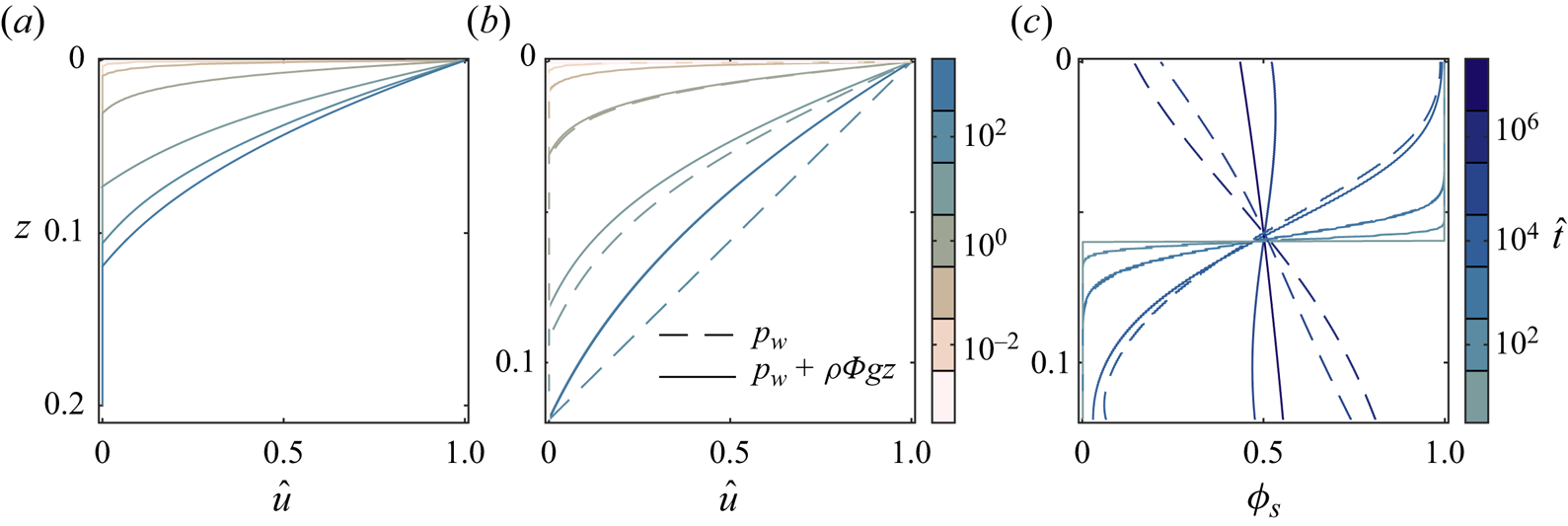
The coupled PDE system in (2.9a,b) is solved using the method of lines (MOL) (Schiesser & Griffiths Reference Schiesser and Griffiths2009). Schaeffer et al. (Reference Schaeffer, Barker, Tsuji, Gremaud, Shearer and Gray2019) used a similar numerical approach as a proof of concept to study compressibility in granular flows. In this work, the robustness of MOL was first tested for the uncoupled segregation equation in (2.5a,b), as validated by Trewhela et al. (Reference Trewhela, Ancey and Gray2021a, figure 13) against the experimental results of van der Vaart et al. (Reference van der Vaart, Gajjar, Epely-Chauvin, Andreini, Gray and Ancey2015). Second, the uncoupled monodisperse granular flow equation in (2.9a) was solved and compared to the solution presented by Cawthorn (Reference Cawthorn2011, figure 2.10) and Jerome & Di Pierro (Reference Jerome and Di Pierro2018) (figure 2a) for  $p_{w}=100$ Pa,
 $u_{w}=1$ m s
 $^{-1}$ and
 $\mu _{w}=0.5$, with the parameters in table 1. The plotted profiles for
 $\hat {u}$ in figure 2(b) also resemble those of Guillard et al. (Reference Guillard, Forterre and Pouliquen2016, figures 2c,e), which were obtained using discrete numerical simulations for
 $g=0$ and
 $g=9.81$ m s
 $^{-2}$ and for a similar flow configuration. This resemblance validates the presented theoretical framework and numerical scheme.
(a) Velocity profile  $\hat {u}$ solutions (2.9a) at different times
 $\hat {t}$ for the monodisperse case (
 $\phi _{s}=0$) and lithostatic pressure distribution with
 $p_{w}=100$ Pa,
 $u_{w}=1$ m s
 $^{-1}$ and
 $\mu _{w}=0.5$, similarly to the solutions found by Cawthorn (Reference Cawthorn2011) and Jerome & Di Pierro (Reference Jerome and Di Pierro2018). (b,c) Comparison of the velocity profiles
 $\hat {u}$ and small particle concentration
 $\phi _{s}$ solutions for different times
 $\hat {t}$ for linear (lithostatic)
 $p=p_{w}+\rho g\varPhi z$ (continuous line) and constant pressure
 $p=p_{w}$ (dashed line) distributions under the same values for the wall parameters
 $u_{w}$,
 $p_{w}$ and
 $\mu _{w}$ with those of (a).

In this work, a particular pressure  $p=p_{w}$ condition is used for the numerical solutions. A linear pressure (lithostatic) distribution adds further complexity to the numerical scheme with no relevant insights into the segregation–rheology feedback. Velocity profiles
 $\hat {u}$ for both pressure distributions are compared in figures 2(b,c) to see the influence of these distributions in the computations. Despite the fact that there are slight differences when comparing the solutions, these are not important compared to the cost of compromising the method's robustness. Pressure is still relevant for segregation (as seen in (2.8) and discussed briefly in Appendix A), but overall segregation dynamics does not change substantially when a constant pressure distribution is imposed over the lithostatic distribution. The latter assumption is particularly justified when considering a highly confined granular bulk, in which case
 $p_{w}\gg \rho _{*}g\varPhi h$. In contrast, the condition where
 $p_{w}$ is neglected in comparison to
 $\rho _{*}g\varPhi z$ poses difficulties to the numerical schemes since segregation velocity
 $f_{sl}\rightarrow \infty$ as
 $z\rightarrow 0$.
Figures 2(b,c) give a first glance at the different time scales at which the segregation–rheology feedback operates. A first time scale is that of momentum diffusion within the granular bulk, related to the granular flow rheology, and visible in the fast development of the velocity profile in figure 2(b). The other two time scales are longer than the former and are related to particle segregation and diffusion processes. These processes are visible in the slow changes of particle concentration profiles  $\phi _{s}$ in figure 2(c).
3. Results
3.1. Effect of size ratio in the segregation and velocity profiles
To demonstrate the crucial role of particle sizes and segregation in the shear flow dynamics, the vertical distributions of small particles  $\phi _{s}$ and horizontal velocity
 $\hat {u}$ are computed as functions of time
 $\hat {t}$ for three particles size ratios
 $R_{d}=\{1.25,2,3.33\}$, keeping
 $p_{w}=100$ Pa,
 $\mu _{w}=0.5$ and
 $u_{w}=0.2$ m s
 $^{-1}$ constant (figure 3). The initially unstable arrangement of small particles over large ones influences the velocity
 $\hat {u}$ profiles; all reach a transient state at
 $\hat {t}\approx 10^{2}$, only to be then altered by segregation. From
 $\hat {t}>10^{2}$, the linear velocity profiles
 $\hat {u}$ for both species, and featuring a slope change at the small–large particle interface, changes into a nonlinear smooth distribution for the final steady-state condition. At initial times, segregation does not influence the velocity profile
 $\hat {u}$ or the time scale to attain the transient linear state. Therefore, momentum transfer is uncoupled from segregation, with the latter acting at longer time scales, an observation made in various experiments and flow configurations (Golick & Daniels Reference Golick and Daniels2009; Tripathi & Khakhar Reference Tripathi and Khakhar2011; van der Vaart et al. Reference van der Vaart, Gajjar, Epely-Chauvin, Andreini, Gray and Ancey2015; Trewhela & Ancey Reference Trewhela and Ancey2021). Nonetheless, size ratio
 $R_{d}$ influences the transient linear state, determining the velocity vertical gradient, a result also observed by Tripathi & Khakhar (Reference Tripathi and Khakhar2011) and corroborated by Barker et al. (Reference Barker, Rauter, Maguire, Johnson and Gray2017). The asymmetric nature of segregation is captured clearly in figures 3(a–c). As the size ratio
 $R_{d}$ increases, small particles segregate faster to the bottom compared to large particles arriving at the top. As a result, when asymmetry
 $\chi _{d}$ is increased, segregation fluxes are fast and dynamic, achieving the nonlinear steady-state swiftly (as observed for
 $R_{d}=3.33$,
 $\chi _{d}=0.7$ in figures 3c,f).
Definition of the parameters used to set the presented numerical simulations in this work. The numerical values for the size asymmetry coefficient  $\chi _{d}$ (hence particle-size ratio
 $R_{d}$) and the frictional asymmetry coefficient
 $\chi _{\mu }$ are used to set the particle parameters. The numerical values for pressure
 $p_{w}$, velocity
 $u_{w}$ and frictional coefficient
 $\mu _{w}$ at the upper plate or wall (see figure 1) resulted in a range of values for
 $h$ (see (2.4)) and set the granular rheology, together with the values of table 1. Finally, the empirical parameters
 $\mathcal {A}$,
 $\mathcal {B}$,
 $\mathcal {E}$ proposed by Trewhela et al. (Reference Trewhela, Ancey and Gray2021a) and Utter & Behringer (Reference Utter and Behringer2004) control the segregation dynamics in the numerical solutions.

(a–c) Vertical and temporal distributions of small particle concentrations  $\phi _{s}$ for
 $u_{w}=0.2$ m s
 $^{-1}$,
 $p_{w}=100$ Pa,
 $\mu _{w}=0.5$ and
 $R_{d}=\{1.25,2,3.33\}$ values. (d–f) Small particle concentration profiles
 $\phi _{s}$ at different
 $\hat {t}$ times for the corresponding
 $R_{d}$ values. (g–i) Velocity profiles
 $\hat {u}$ at different
 $\hat {t}$ instants for the corresponding
 $R_{d}$ values, reflected in its asymmetrical coefficient
 $\chi _{d}=(R_{d}-1)/R_{d}$ value. The thicker line in each of (d–i) highlights the final solution of each profile. Animated solutions of (d–i) are in supplementary movie 1, available at https://doi.org/10.1017/jfm.2024.168.

Other striking differences appear when comparing the final small particle concentrations  $\phi _{s}$. Larger
 $R_{d}$ values produce sharper profiles with strongly segregated
 $\phi _{s}$ profiles and a marked small–large interface. Subsequently, this segregated and nonlinear distribution is imprinted into the shape of the steady-state velocity profile
 $\hat {u}$, thus a direct result of particle-size segregation effectiveness. For size ratios
 $R_{d}\rightarrow 1$, apparent mixing (i.e. diffusive remixing) is observed. Controlled by diffusion, mild segregation produces quasi-linear
 $\hat {u}$ profiles, as shown in figure 3(d). In contrast to these quasi-linear profiles,
 $\hat {u}$ solutions for large
 $R_{d}$ show a sharp break in the velocity profile, drawing a rhomboid or lens geometry. The rhomboid is defined graphically by the linear responses expected for the normally graded and inversely graded conditions for particle-size distribution.
3.2. Initially mixed conditions and resulting profiles
The normally graded condition shown in figure 1(a) is a widely explored initial condition for segregation in experiments and numerical simulations (e.g. van der Vaart et al. Reference van der Vaart, Gajjar, Epely-Chauvin, Andreini, Gray and Ancey2015; Gray Reference Gray2018; Chassagne et al. Reference Chassagne, Maurin, Chauchat, Gray and Frey2020). However, in the context of mixed bidisperse granular flows, the initially mixed condition illustrated in figure 1(b) also provides a valuable assessment on how segregation affects the rheology of granular mixtures. Figure 4 shows the resulting small particle concentration  $\phi _{s}$ and velocity
 $\hat {u}$ profiles for three different initially mixed conditions of small and large particles at
 $\phi _{s}^{0}=25$, 50 and 75 % homogeneously mixed concentrations. To compare with the results shown previously in figures 3(c,f,i), an
 $R_{d}=3.33$ value is used. The steady state
 $\phi _{s}$ distribution and the
 $\hat {u}$ profile observed in figures 4(b,e,h) are identical to those observed in figures 3(c,f,i). This agreement proves that steady-state solutions are independent of the normally graded or mixed initial conditions. Such independence is just about the particles’ initial arrangement, and it is not extended to the average particle concentration
 $\phi _{s}^{0}$, a condition that results in differing profiles for
 $\phi _{s}$ and
 $\hat {u}$ (figure 4).
(a–c) Vertical and temporal distributions of small particle concentrations  $\phi _{s}$ for
 $u_{w}=0.2$ m s
 $^{-1}$,
 $p_{w}=100$ Pa,
 $\mu _{w}=0.5$ and
 $R_{d}=3.33$ for initially-mixed conditions of small and large particles,
 $\phi ^{0}_{s}=\{0.25,0.5,0.75\}$. (d–f) Small particle concentration
 $\phi _{s}$ and (g–i) velocity
 $\hat {u}$ profiles at different
 $\hat {t}$ instants for the corresponding
 $\phi _{s}^{0}$ and the same wall parameters and
 $R_{d}$ value. The thicker line in each of (d–i) highlights the final solution of each profile. Animated solutions of (d–i) are available in supplementary movie 2.

As expected, there are important differences in the intermediate solutions for both  $\phi _{s}$ and
 $\hat {u}$ due to the change in the initial conditions. Homogeneously mixed initial
 $\phi _{s}^{0}$ concentrations produce not only different velocity
 $\hat {u}$ and skewed – but similar –
 $\phi _{s}$ profiles, but also delay segregation. The delayed steady-state solutions observed in figures 4(a–c) for larger
 $\phi _{s}^{0}$ concentrations are tied inherently to the asymmetric nature of size segregation, i.e. the segregation flux
 $\boldsymbol {F}_{s}=f_{sl}\phi _{s}\phi _{l}\boldsymbol {g}/|\boldsymbol {g}|\sim (1-\chi _{d}\phi _{s})^{2}\phi _{s}(1-\phi _{s})$. Small particles at low
 $\phi _{s}$ concentrations segregate at a faster rate than large particles at low
 $\phi _{l}$ concentrations (Gajjar & Gray Reference Gajjar and Gray2014; van der Vaart et al. Reference van der Vaart, Gajjar, Epely-Chauvin, Andreini, Gray and Ancey2015; Trewhela et al. Reference Trewhela, Ancey and Gray2021a). If segregation fluxes were to be symmetric
 $\boldsymbol {F}_{s}= \phi _{s}\phi _{l}\boldsymbol {g}/|\boldsymbol {g}|$, then segregation rate would be maximum at
 $\phi _{s}^{0}=0.5$, and at identical rates for
 $\phi _{s}^{0}=\{0.25,0.75\}$ (Gray Reference Gray2018). Therefore, figure 4 reproduce the expected asymmetry. For
 $\phi _{s}^{0}=0.25$, segregation alters the velocity profile solution swiftly from the mixed condition (at
 $\hat {t}\approx 10^{2}$) into the steady-state condition at almost
 $\hat {t}\approx 10^{4}$. In the case of
 $\phi _{s}^{0}=0.75$, segregation also initiates at
 $\hat {t}\approx 10^{2}$, but steady-state solutions are reached at a slower pace, i.e. at
 $\hat {t}\approx 10^{5}$. These differences hint at a
 $\phi _{s}$-dependent time scale for segregation that controls the final duration of the segregation–rheology feedback.
3.3. Influence of differences in the particles’ frictional coefficients
An additional effect in the Stokes’ problem is explored by changing the small particles’ frictional coefficient  $\mu _{s}$ while keeping the size ratio
 $R_{d}=2$ fixed, along with
 $p_{w}=300$ Pa,
 $\mu _{w}=0.5$ and
 $u_w=0.2$ m s
 $^{-1}$. Differences in
 $\mu _{s}$, relative to
 $\mu _{l}$ via
 $R_{\mu }$, introduce a non-zero
 $\chi _{\mu }$ value in (2.9a), which is null when small and large particles share the same
 $\mu (I)$-rheology parameters (table 1). Changes in
 $\chi _{\mu }$ lead to velocity differences at the small–large particles interface, compromising the numerical scheme due to
 $\hat {u}$ discontinuity. Numerical solutions are found only for slight changes in
 $\chi _{\mu }$, within the interval
 $\chi _{\mu }=[-0.033,0.013]$ for
 $R_{d}=2$. This interval depends on the size ratio as well; as the size ratio
 $R_{d}$ increases, the
 $\chi _{\mu }$ interval for the solutions narrows.
In figure 5,  $\phi _{s}$ and
 $\hat {u}$ solutions are plotted for various
 $\chi _\mu$ values. While the small particle concentration
 $\phi _{s}$ solutions do not show significant differences between the different
 $\chi _\mu$ cases, the velocity profiles
 $\hat {u}$ display interesting behaviour. For negative
 $\chi _\mu$ values,
 $\mu _{s}$ is larger than
 $\mu _{l}$, resulting in the transient solution having inverted slopes compared to the case with positive
 $\chi _\mu$ values; see figures 5(f,j) for comparison. Intermediate negative values for
 $\chi _\mu$ seem to counteract the
 $\hat {u}$ profile nonlinearity generated by the size difference in
 $R_{d}$ (figures 5g,h). This finding is consistent with the proposed theoretical framework and could illustrate a way to obtain linear velocity profiles in granular flows with particles of varying sizes and frictional properties. Therefore, to control the particles’ frictional properties is to partially control the segregation–rheology feedback, despite having a segregated bulk with different grain sizes.
Numerical solutions for (a–e) small particle concentrations  $\phi _{s}$, and (f–j) velocity profiles
 $\hat {u}$ with constant wall parameters
 $u_{w}=0.2$ m s
 $^{-1}$,
 $p_w=300$ Pa,
 $\mu _{w}=0.5$,
 $R_{d}=2$, and variable
 $\chi _{\mu }=\{-0.03,-0.02,-0.01,0,0.01\}$ for (a,f), (b,g), (c,h), (d,i) and (e,j), respectively. The thicker line in each plot highlights the final solution of each variable. Solutions plotted in (d,f–j) are shown as animations in supplementary movie 3.

3.4. Steady-state analytical solutions and comparison with numerical solutions
A solution for the transient velocity profiles  $\hat {u}$ can be determined analytically from the steady-state condition in (2.9a), i.e.
 $\bar {\mu }=\mu _{w}$. This condition is replaced in the quadratic expression for
 $I$, obtained from the regularized
 $\mu (I)$-rheology in (2.2):
 \begin{equation} \mu_{\infty}I^{2}+(\mu_{2}-\mu_{w})I+(\mu_{1}-\mu_{w})I_{0}=0.\end{equation}
The positive solution for  $I$ is then balanced with the inertial number
 $I$ definition to yield a differential equation for the velocity
 $\hat {u}$. This ODE is solved by separating variables and using the no-slip boundary condition
 $\hat {u}|_{\hat {z}=1}=0$ to yield
 \begin{equation} \hat{u}=\frac{h}{u_{w}\bar{d}}\,\sqrt{\frac{p_{w}}{\rho_{*}}}\, \mathcal{I}(\mu_{w})\,(1-\hat{z}),\end{equation}
where  $\mathcal {I}(\mu _{w})=((\mu _{w}-\mu _{2})+\sqrt {(\mu _{w}- \mu _{2})^{2}+4\mu _{\infty }(\mu _{w}-\mu _{1})I_{0}})/2\mu _{\infty }$ is the aforementioned positive solution of (3.1), i.e. the inertial number
 $I$. Equation (3.2) results in the rhomboid formation, already described and discussed in § 3.1. If the concentration-averaged diameter
 $\bar {d}$ is evaluated with the normally-graded size distribution,
 $\phi _{s}\big |_{\hat {z}=0}^{\hat {z}=1/2}=1$ and
 $\phi _{s}\big |_{\hat {z}=1/2}^{\hat {z}=1}=0$, and the inversely-graded size distribution,
 $\phi _{s}\big |_{\hat {z}=0}^{\hat {z}=1/2}=0$ and
 $\phi _{s}\big |_{\hat {z}=1/2}^{\hat {z}=1}=1$, then the rhomboid can be diagrammed. The solution captured by (3.2) provides a good approximation of the transient velocity profile without considering segregation in its development. When segregation determines the velocity profile, a steady-state solution for the small particle concentration
 $\phi _{s}$ can be obtained. For that, the procedure used by Trewhela et al. (Reference Trewhela, Ancey and Gray2021a) is followed, yet their solution is implicit for
 $\phi _{s}$. Here, a simpler differential equation is developed from
 $\mathcal {E}=0$ (a first-order approximation in
 $R_{d}-1$), resulting in the explicit solution
 \begin{equation} \phi_{s}=\frac{{\rm e}^{(\hat{z}+\mathcal{K})/\lambda}}{1+ {\rm e}^{(\hat{z}+\mathcal{K})/\lambda}},\end{equation}
where  $\mathcal {K}=-1/2$ is the constant of integration, which can be calculated using the depth-averaged condition
 $\bar {\phi }_{s}=\int ^{1}_{0}\phi _{s}\,\text {d}\hat {z}=0.5$, and
 $\lambda =\mathcal {A}p_{w}/(\mathcal {B}\rho g h(R_{d}-1))$. This small particle concentration
 $\phi _{s}$ profile serves as input for the generalized ODE:
 \begin{equation} \frac{\text{d}\hat{u}}{\text{d}\hat{z}}=-\frac{h}{u_{w}\bar{d}}\,\sqrt{\frac{p_{w}}{\rho_{*}}}\,\mathcal{I}(\hat{\mu}_{w}), \end{equation}
where  $\hat {\mu }_{w}=\mu _{w}(1-2.7(1-\phi _{s})\chi _{\mu })/(1-\chi _{\mu }\phi _{s})$ is a
 $\phi _{s}$- and
 $\chi _{\mu }$-dependent frictional coefficient, with
 $\bar {d}$ a function of the former as well. Due to this dependence, the ODE's solution is computed using a Runge–Kutta fourth-order method.
Figure 6 summarizes the core behaviour of the segregation–rheology feedback. The transient-state solution of (3.2) and its reciprocal stable state (red and blue toned rhomboids) are shown in figure 6(a). These rhomboids emphasize the slope change in  $\hat {u}$ as
 $R_{d}$ increases, with the fully linear case
 $R_{d}=1$ as reference. In figure 6(b), the generalized solution in (3.4) is drawn for the
 $R_{d}=2$ case and various
 $\chi _{\mu }$ values, with the reference curve
 $\chi _{\mu }=0$ at the middle. Negative
 $\chi _{\mu }$ values tend to displace the steady-state velocity profile
 $\hat {u}$ towards the linear reference, acting as a counterpart for the deviation generated by the size ratio
 $R_{d}$. Conversely, positive
 $\chi _{\mu }$ values exacerbate the nonlinear behaviour of the velocity profiles
 $\hat {u}$, displacing the curves beyond the reciprocal stable-state curve (with large particles over small ones). Moreover, solutions attempting to pass beyond the stable state could explain the difficulties in obtaining solutions when the frictional asymmetric coefficient is
 $\chi _\mu >0.013$ for
 $R_{d}=2$. A detailed evolution of the velocity profile
 $\hat {u}$ solutions is shown in figure 6(c). The velocity profile
 $\hat {u}$ develops from the initial condition to the transient state
 $\hat {t}\sim 10^{2}$, adjusting well to the analytical solution of (3.2) (left rhomboid linear curves in figure 6(c), taken from
 $R_{d}=2$ in figures 6a,b). Then segregation alters this state, rearranging particles according to their size, achieving a steady state at
 $\hat {t}\approx 10^{5}$ that fits well the ODE solution in (3.4) (dot-dashed line in figure 6c). In figure 6(c) the segregation–rheology feedback ends up being described graphically by the changes in
 $\hat {u}$ from the transient to the steady state, hence analytically bounded within the
 $R_{d}$-dependent rhomboid region.
(a) Velocity profiles  $\hat {u}$ for the steady-state condition in (3.2) for various
 $R_{d}=[1,4]$ values, represented in blue and red tones for
 $d_{s}$ and
 $d_{l}$, respectively. (b) Velocity profiles
 $\hat {u}$ of the numerically solved (3.4) for variable
 $\chi _{\mu }=[-0.05,0.05]$ and constant
 $R_{d}=2$, with its corresponding rhomboid from (a). (c) Temporal evolution of the velocity profile
 $\hat {u}$ for the
 $R_{d}=2$ and
 $\chi _{\mu }=0.01$ case compared with the corresponding steady-state solutions from (a) ((3.2), plotted as a rhomboid) and (b) ((3.4), plotted with a dot-dashed line). Note how the velocity profiles
 $\hat {u}$ first collapse around the rhomboid solution, and then converge to the steady-state solution (red dot-dashed line). Fully animated solutions (for
 $\chi _{\mu }=\{-0.03,-0.01,0.01\}$ and constant
 $R_{d}=2$), compared to the steady-state solutions of (3.2) and (3.4), are shown in supplementary movies 4–6.

3.5. Granular kinematic viscosity, time scales and segregation–momentum balances
From the ODE for the non-dimensional shear rate  $\hat {\dot {\gamma }}=|\text {d}\hat {u}/\text {d}\hat {z}|$ in (3.4), a general definition for the granular kinematic viscosity
 $\nu _{g}$ can be formulated. Using the theoretical constitutive relation for a granular dynamic viscosity
 $\tau =\mu p=\eta _{g}\dot {\gamma }$ (Jing et al. Reference Jing, Ottino, Umbanhowar and Lueptow2022), the dimensional kinematic viscosity can be defined as
 \begin{equation} \nu_{g}=\frac{\hat{\mu}_{w}\bar{d}}{\mathcal{I}(\hat{\mu}_{w})}\, \sqrt{\frac{p_{w}}{\rho_{*}}}.\end{equation}
Compared to the granular viscosity definition of Jerome & Di Pierro (Reference Jerome and Di Pierro2018), in (3.5) this bidisperse granular viscosity is  $R_{d}$-,
 $\chi _{\mu }$- and
 $\phi _{s}$-dependent (via
 $\bar {d}$ and
 $\hat {\mu }_{w}$), and is still determined by the wall conditions and the
 $\mu (I)$-rheology parameters (table 1). It is worth recalling that the
 $\mathcal {I}$ function is in fact the inertial number
 $I$, but for the Stokes’ problem analysed in this work, it is left as the function defined in (3.2).
The definition of  $\nu _{g}$ allows the analysis of the different time scales at which the segregation–rheology feedback develops. Evidently, a first time scale appears from the non-dimensional time
 $\hat {t}$ definition, where
 $t_{\dot {\gamma }}\sim h/u_{w}$ can be defined as a convective or shear rate time scale, inferred from
 $1/\dot {\gamma }=(\text {d}u/\text {d}z)^{-1}\approx h/u_{w}$ (as in the definition of
 $I$; GDR-MiDi 2004). A second time scale can be associated with momentum diffusing through the granular bulk and derived directly from (3.5), yielding
 \begin{equation} t_{\nu_{g}}\sim \frac{h^{2}}{\nu_{g}}=\frac{h^{2}\,\mathcal{I}(\hat{\mu}_{w})}{\hat{\mu}_{w} \bar{d}}\,\sqrt{\frac{\rho_{*}}{p_{w}}}.\end{equation}
Then two more time scales appear from the particle-segregation-related processes. A segregation time scale is drawn by the time it takes particles of diameter  $\bar {d}$ to segregate through the sheared layer
 $h$ with velocity
 $f_{sl}$:
 \begin{equation} t_{f_{sl}}\sim \frac{h}{f_{sl}}=n_{\bar{d}}P\,\mathcal{F}(R_{d},\phi_{s})^{-1}\,t_{\dot{\gamma}}, \end{equation}
where  $n_{\bar {d}}=h/\bar {d}$ is the number of particle layers through the sheared layer depth,
 $\mathcal {F}(R_{d},\phi _{s})=\mathcal {B}(R_{d}-1)[1+\mathcal {E}(R_{d}-1)(1-\phi _{s})]$ is a function defined from the segregation velocity
 $f_{sl}$ function, and
 $P=p_{w}/(\rho _{*}g\bar {d})$ corresponds to a non-dimensional pressure (Trewhela et al. Reference Trewhela, Ancey and Gray2021a). The segregation time scale is proportional to
 $t_{\dot {\gamma }}$ and
 $p_{w}$, in agreement with the clear segregation dependence on shear rate and pressure (Golick & Daniels Reference Golick and Daniels2009; Trewhela et al. Reference Trewhela, Gray and Ancey2021b). Thus the segregation time scale
 $t_{f_{sl}}$ is the shear rate time scale
 $t_{\dot {\gamma }}$ modulated by pressure conditions at the wall, segregation, and the number of layers that particles must segregate through. Finally, the particle diffusion time scale can be defined as
 \begin{equation} t_{\mathcal{D}_{sl}}\sim \frac{h^{2}}{\mathcal{D}_{sl}}= \frac{n_{\bar{d}}^{2}}{\mathcal{A}}\,t_{\dot{\gamma}}, \end{equation}
which again is proportional to  $t_{\dot {\gamma }}$. Although these time scales do not provide the actual time that the velocity
 $\hat {u}$ and small particle concentration
 $\phi _{s}$ profiles take to reach their corresponding steady-state solutions, which is out of the scope of this work, they serve to describe the progression of the segregation–rheology feedback.
For the numerical solutions computed in § 3.1,  $t_{\dot {\gamma }}=0.0157$ s and the momentum diffusion time scale share similar values
 $t_{\nu _{g}}\approx 0.15$ s, yielding a non-dimensional time
 $\hat {t}=t_{\nu _{g}}/t_{\dot {\gamma }}\approx 10$ for the
 $\hat {u}$ profiles to develop into the transient solution. This value is close to what is shown in figure 3, with
 $\hat {t}\approx 10^2$ being the time at which the transient solution is achieved in the computations. In terms of segregation, there are larger differences in
 $t_{f_{sl}}\approx \{100,20,7\}$ s and
 $t_{\mathcal {D}_{sl}}=\{80,120,170\}$ s for
 $R_{d}=\{1.25,2,3.33\}$, respectively. These
 $t_{f_{sl}}$ values capture well the faster set in of segregation at
 $\hat {t}=t_{f_{sl}}/t_{\dot {\gamma }} \approx \{6\times 10^{3},10^{3},5\times 10^{2}\}$ for the same
 $R_{d}$ values. However, these
 $t_{f_{sl}}$ are balanced out by shorter or larger diffusive time scales
 $t_{\mathcal {D}_{sl}}$, which finally settle the concentration profiles into their steady-state solution. Consistent results are observed when analysing these time scales in the case of the initially mixed condition solutions at fixed
 $R_{d}=3.33$. These yield the same
 $t_{\dot {\gamma }}$ and
 $t_{\nu _{g}}$ values for all solutions, but
 $t_{f_{sl}}\approx \{3,7,20\}$ s and
 $t_{\mathcal {D}_{sl}}\approx \{100,170,310\}$ s increase with
 $\phi _{s}^{0}=\{0.25,0.5,0.75\}$, resulting in the monotonic increase of
 $\hat {t}=t_{\mathcal {D}_{sl}}/t_{\dot {\gamma }} \approx \{7\times 10^3,10^4,2\times 10^4\}$. These values are also similar to the times found in the numerical solutions (figure 4). In the case of the varying
 $\chi _\mu$ solutions, there are only slight differences in
 $t_{\nu _{g}}$. Values decrease from approximately 0.9 s to 0.7 s as
 $\chi _\mu$ goes from
 $-$0.03 to 0.01.
From these results and the analysed time scales, it is thus natural to compare the two diffusion processes acting in the bidisperse granular Stokes’ problem. With the definition of the granular momentum diffusivity time scale, or its diffusivity coefficient in  $\nu _{g}$, the Schmidt number or the ratio of the momentum and particle diffusivity time scales is obtained directly as
 \begin{equation} Sc=\frac{t_{\nu_{g}}}{t_{\mathcal{D}_{sl}}}=\frac{\nu_{g}}{\mathcal{D}_{sl}}= \frac{\hat{\mu}_{w}}{\mathcal{A}I^{2}}, \end{equation}
where the inertial number is reintroduced for simplicity and generalization; for that matter,  $I$ can be considered equal to
 $d\dot {\gamma }/\sqrt {p/\rho _*}$ or equal to the definition of
 $\mathcal {I}$ made after (3.2). It is worth noting that the
 $I^{2}$ term corresponds to the Savage or Coulomb number (Savage Reference Savage1984; Ancey, Coussot & Evesque Reference Ancey, Coussot and Evesque2000). Low
 $Sc$ values indicate an important particle diffusivity (diffusive remixing), dominating over momentum diffusion, which at first glance can be achieved with low
 $\mu _{w}$, high
 $\mathcal {A}$ or high inertial numbers
 $I$. Conversely, a large
 $Sc$ points towards a more viscous response from the granular material, with a lesser role played by particle diffusion in the overall flow dynamics. Interestingly, this definition of the Schmidt number depends implicitly not only on the particles’ concentration-averaged diameter
 $\bar {d}$ (via
 $I$), hence their size ratio
 $R_{d}$ and size asymmetry coefficient, but also on the frictional asymmetry coefficient
 $\chi _{\mu }$ and the particles’ frictional parameters.
To illustrate these dependencies, figure 7(a) shows the Schmidt number  $Sc$ as a function of both
 $\mu _{w}$ and an overall small particle concentration, which can be interpreted as the initial small particle concentration
 $\phi _{s}^{0}$ or the depth-averaged small particle concentration
 $\overline {\phi _{s}}=\int _{0}^{1}\phi _{s}\,\text {d}\hat {z}$. In figure 7(a), the contours’ slope is determined by
 $\chi _{\mu }$: positive
 $\chi _{\mu }$ yields a negative slope (dashed contours), and vice versa (filled contours). For the computed values in the domain
 $\mu _{w}=[0.4,1.2]$ and
 $\phi _{s}=[0,1]$,
 $Sc$ varies from
 $10^{3}$ to
 $10^{-1}$, decreasing linearly in two regions marked approximately by
 $\mu _{w}\lessgtr \mu _{2}=0.557$. This is a direct result of the partially regularized
 $\mu (I)$-rheology, which allows
 $\mu _{w}>\mu _{2}$, therefore extending the range for
 $Sc$. Overall,
 $Sc$ decreases with
 $\mu _{w}$, and increases slightly with higher
 $\phi _{s}^{0}$, when
 $\chi _{\mu }<0$. The former observation contradicts the linear dependence of
 $Sc$ on
 $\mu _{w}$, but is consistent with the fact that high
 $\mu _{w}$ values result in high
 $I$ values as well, since
 $Sc\sim I^{-2}$. (For more results shedding light on the role of
 $\mu _{w}$, see Appendix A.) While particle diffusivity scales with the shear rate
 $\mathcal {D}_{sl}\sim \dot {\gamma }$ (Utter & Behringer Reference Utter and Behringer2004), the granular viscosity scales inversely with the latter
 $\nu _{g}\sim \dot {\gamma }^{-1}$; so larger friction at the wall produce high shear rates and will result in low
 $Sc$. But as stated before, the segregation–rheology feedback is not a purely momentum- or particle-diffusion-dominated process; segregation also controls the flow dynamics.
(a) Filled contours for the Schmidt number  $Sc=t_{\nu _{g}}/t_{\mathcal {D}_{sl}}=\nu _{g}/\mathcal {D}_{sl}$ as a function of both
 $\mu _{w}$ and the overall small particle concentration
 $\phi _{s}^{0}$, in the case
 $\chi _{\mu }=-0.03$. Dashed contours show the change of slope in the case
 $\chi _{\mu }=0.03$ for the same
 $Sc$ values of the filled contours. (b) Filled contours for the segregation–rheology Péclet number
 $Pe_{sr}=t_{f_{sl}}/t_{\nu _{g}}=hf_{sl}/\nu _{g}$ as a function of
 $\mu _{w}$ and the size ratio
 $R_{d}$, in the case
 $\chi _{\mu }=0.01$. (c) Variation of the segregation–rheology Péclet number
 $Pe_{sr}$ as a function of the wall friction
 $\mu _{w}$ and the frictional asymmetry parameter
 $\chi _{\mu }$. For comparison, the constant frictional parameter
 $\mu _{2}=0.557$ is plotted alongside the same
 $Pe_{sr}$, but using the non-regularized inertial number definition
 $\mathcal {I}_{nr}=I_{0}(\mu _{w}-\mu _{1})/(\mu _{2}-\mu _{w})$, which is independent of
 $\chi _{\mu }$ (dot-dashed thick line).

To understand better at which extent segregation controls the segregation–rheology feedback, a particle segregation–diffusion balance is borrowed from previous work. Following the definitions made by Gray (Reference Gray2018) and Trewhela et al. (Reference Trewhela, Ancey and Gray2021a), a Péclet number for segregation  $Pe$ can be defined as the ratio between the segregation velocity
 $f_{sl}$ and particles’ diffusivity
 $\mathcal {D}_{sl}$, i.e.
 $Pe=hf_{sl}/\mathcal {D}_{sl}$, or alternatively,
 $t_{f_{sl}}/t_{\mathcal {D}_{sl}}$. With this definition, a specific Péclet number for the segregation–rheology feedback can be introduced as
 \begin{equation} Pe_{sr}=\frac{Pe}{Sc}=\frac{hf_{sl}}{\nu_{g}}= \frac{t_{f_{sl}}}{t_{\nu_{g}}}=\frac{I^{2}}{\varPhi_{p} \hat{\mu}_{w}}\,\mathcal{F}(R_{d},\phi_{s}), \end{equation}
where  $\varPhi _{p}=p_{w}/(\rho g h)$ is a non-dimensional pressure, which can be interpreted as an equivalent solids volume fraction. Again, this second non-dimensional quantity depends on
 $I^{2}$ (or the Savage number). Compared to the previous
 $Sc$ definition, the segregation–rheology Péclet number
 $Pe_{sr}$ depends on the size ratio
 $R_{d}$ and the empirical constants determined by Trewhela et al. (Reference Trewhela, Ancey and Gray2021a). The proposed
 $Pe_{sr}$ somehow confirms the results discussed previously in §§ 3.1 and 3.3, where segregation profiles were sharper for large
 $R_{d}$ (figure 3) and positive
 $\chi _{\mu }$ values (figure 5).
Figures 7(b,c) show the variation of the segregation–rheology Péclet number  $Pe_{sr}$ as a function of
 $\hat {\mu }_{w}$,
 $\mu _{w}$ and
 $R_{d}$. Broadly, the
 $Pe_{sr}$ dependence on
 $R_{d}$ is well captured in figure 7(b). As expected,
 $Pe_{sr}$ is minimum for
 $R_{d}\rightarrow 1$, and interestingly, larger size differences do not necessarily result in predominant segregation effects over momentum diffusion, since
 $Pe_{sr}=0.01$ for
 $R_{d}=4$ and
 $\mu _{w}=0.4$. Therefore, the results presented in the previous subsections are summarized conceptually in the
 $Pe_{sr}$ definition; the segregation–rheology feedback is relevant when a combination of both high friction and large size differences is in place. Nonetheless, high
 $\mu _{w}$ is still enough to promote segregation, even accompanied by low
 $R_{d}$. All this, as long as there is sufficient pressure
 $p_{w}$ or the bulk is compressed (
 $\varPhi _{p}$) enough at the wall to transfer shear without restraining both momentum and segregation. The latter opens the possibility of including compressibility effects in the proposed system and solutions. In figure 7(c), the
 $Pe_{sr}$ curves are plotted for various
 $\chi _{\mu }$ values, all of which show similar behaviour. However, when
 $Pe_{sr}$ is calculated using the non-regularized
 $\mu (I)$-rheology, i.e.
 $\mathcal {I}_{nr}=I_{0}(\mu _{w}-\mu _{1})/(\mu _{1}-\mu _{w})$, the
 $Pe_{sr}$ value diverges as
 $\mu _{w}\rightarrow \mu _{2}$ (thick dashed line in figure 7c). This shows the importance of having a well-posed extended formulation for the
 $\mu (I)$-rheology. When using the partially regularized
 $\mu (I)$-rheology,
 $Pe_{sr}$ continues to increase monotonically with
 $\mu _{w}>\mu _{2}$, but at a lower rate than for
 $\mu _{w}<\mu _{2}$, and without a clear cutoff value.
4. Conclusions
The segregation–rheology feedback in dense granular flows was explored numerically and theoretically via Stokes’ first problem for a bidisperse granular bulk at constant solids volume fraction. Using this paradigmatic problem for such a nonlinear and coupled system required the implementation of the method of lines, which proved to be a practical numerical scheme despite the issues inherited from the  $\mu (I)$-rheology implementation. The solved PDE system incorporated the partially regularized
 $\mu (I)$-rheology of Barker & Gray (Reference Barker and Gray2017) and the scaling law for bidisperse size segregation of Trewhela et al. (Reference Trewhela, Ancey and Gray2021a). The results focused on the role of size ratio
 $R_{d}$ in the development of velocity profiles, and included the effect of frictional differences or a frictional ratio
 $R_{\mu }$ between particle species via the introduced parameter
 $\chi _{\mu }=(R_{\mu }-1)/R_{\mu }$, in analogy with the segregation asymmetry coefficient
 $\chi _{d}=(R_{d}-1)/R_{d}$. Under a constant pressure
 $p_{w}$ condition, the numerical solutions showed a transient state, decoupled from the segregation process, achieving linear velocity profiles
 $\hat {u}$. Then segregation-induced feedback alters particle concentrations, thus changing the linear
 $\hat {u}$ state into a
 $\phi _{s}$- and
 $R_{d}$-dependent nonlinear solution for
 $\hat {u}$. The transient and steady-state solutions encompass a rhomboid region that expands as
 $R_{d}$ increases, and reduces to a single linear profile when
 $R_{d}\rightarrow 1$ (with no segregation). The steady-state solution is determined not only by
 $R_{d}$ but also by the particles’ frictional coefficient ratio
 $R_{\mu }$. While positive
 $\chi _\mu$ values exacerbate the solutions’ nonlinearity, negative values of
 $\chi _{d}$ dampen the effect of
 $R_{d}$ and favour a linear behaviour, counteracting the segregation-induced feedback. The numerical solutions converge well around the analytical expressions (3.2) and (3.4), which bound the feedback's solution range.
The kinematic granular viscosity  $\nu _{g}$ was redefined based on the partially regularized
 $\mu (I)$-rheology and the concentration-averaged diameter
 $\bar {d}$, hence determined locally by particle concentrations
 $\phi _{\nu }$. Four characteristic time scales arising from shear rate
 $t_{\dot {\gamma }}$, granular momentum diffusion
 $t_{\nu _{g}}$, segregation
 $t_{f_{sl}}$ and particle diffusion
 $t_{\mathcal {D}_{sl}}$ were introduced to describe the progression of the segregation–rheology feedback. These time scales did not provide precise expressions for the time at which the variables attained the transient and steady states, but explained well the observed temporal differences in the presented numerical results. From
 $\nu _{g}$ and these four time scales, two non-dimensional numbers appeared naturally as a result of segregation–momentum balances: a Schmidt number
 $Sc=\nu _{g}/\mathcal {D}_{sl}$, and a specific segregation–rheology Péclet number
 $Pe_{sr}=hf_{sl}/\nu _{g}$. These two quantities not only showed consistency with the numerical and theoretical results, but also provided a broad description for the segregation–rheology feedback and its dependence on the plethora of parameters addressed here.
Although the coupled Stokes’ problem is an idealized case study, the developed analyses provide a robust numerical scheme for particle-size segregation in granular flows that is easy to compare with experimental results and applicable to the rheometry of dense granular flows (e.g. Golick & Daniels Reference Golick and Daniels2009; Trewhela & Ancey Reference Trewhela and Ancey2021). Particle-size segregation and local friction redistribution, as discussed in this work, may have consequences for the scales associated with shear bands (May et al. Reference May, Golick, Phillips, Shearer and Daniels2010), or other processes like jamming (Rietz & Stannarius Reference Rietz and Stannarius2008). Further research is required to extend this feedback analysis towards an extended range of size ratios and flow characteristics – compressibility, reverse segregation or other segregation mechanisms – that are still not considered but could complement or fit well in the presented approach (Schaeffer et al. Reference Schaeffer, Barker, Tsuji, Gremaud, Shearer and Gray2019; Neveu et al. Reference Neveu, Larcher, Delannay, Jenkins and Valance2022).
Supplementary movies
Supplementary movies are available at https://doi.org/10.1017/jfm.2024.168.
Acknowledgements
The author thanks J. Dumais, J.M.N.T. Gray, L. Gordillo and H. Ulloa for their constructive comments on this paper. The colour maps used in this paper are readable by both colour-vision-deficient and colour-blind people (Crameri Reference Crameri2018).
Funding
This research received support from Agencia Nacional de Investigación y Desarrollo (ANID) through FONDECYT Iniciación Project 11240630, Dirección de Investigación of Universidad Adolfo Ibañez through Programa de Apoyo a la Investigación, and Facultad de Ingeniería y Ciencias through their Startup Package.
Declaration of interests
The author reports no conflict of interest.
Appendix A. Role of wall parameters  $p_{w}$, $u_{w}$ and $\mu _{w}$


The segregation–rheology feedback is dominated primarily by the particles’ size ratio  $R_{d}$ and the frictional asymmetry coefficient
 $\chi _{\mu }$. The pressure
 $p_{w}$, velocity
 $u_{w}$ and frictional coefficient
 $\mu _{w}$ at the wall also influence and control both the segregation and rheology, through shear and pressure, hence the inertial number
 $I$. Roughly, in the numerical solutions, the combination of these three wall parameters tunes the rate at which momentum is transferred into the bulk. To address the role of each of these parameters, a set of solutions is obtained for variable
 $p_{w}$,
 $u_{w}$ and
 $\mu _{w}$ values while keeping the rest of the parameters constant, including
 $R_{d}$ and
 $\chi _{\mu }$, which were set to 2 and 0, respectively. Figure 8 shows the results of varying these parameters, and the effect they have on the resulting profiles for the explored Stokes’ problem. The results can be separated into three subsets of solutions, one for each varying parameter.
Influence of wall parameters in small particle concentrations  $\phi _{s}$ (top row) and velocity profiles
 $\hat {u}$ (bottom row) for: (a–d) variable wall pressure
 $p_{w}=\{100,10\ 000\}$ Pa and constant wall velocity
 $u_{w}=1$ m s
 $^{-1}$ and frictional coefficient
 $\mu _{w}=0.8$; (e–h) variable wall velocity
 $u_{w}=\{0.1,10\}$ m s
 $^{-1}$ and constant wall pressure
 $p_{w}=1000$ Pa and frictional coefficient
 $\mu _{w}=0.8$; and (i–l) variable wall frictional coefficient
 $\mu _{w}=\{0.4,1.2\}$ and constant wall pressure
 $p_{w}=1000$ Pa and velocity
 $u_{w}=1$ m s
 $^{-1}$. In these solutions,
 $\chi _{d}=0$, with the empirical parameters in tables 1 and 2. The thicker line in each plot highlights the final profile of each variable.

A direct comparison between figures 8(a,b) and 8(c,d) indicates that larger  $p_{w}$ values enhance the transfer of momentum, while restraining segregation, hence stretching the duration of the segregation–rheology feedback. Some of these observations made for
 $p_{w}$ are inverted in the case of
 $u_{w}$. In the case
 $u_{w}=0.1$ m s
 $^{-1}$ in figure 8(e), the transient
 $\hat {u}$ profile is achieved swiftly with the resulting shear rate
 $\dot {\gamma }$. Yet this has little effect on the segregation velocity. Since
 $f_{sl}\sim \dot {\gamma }$, segregation takes longer for low
 $\dot {\gamma }$, hence delaying the segregation–rheology feedback, as observed in figure 8(f). Conversely, as figure 8(g) shows, larger
 $u_{w}$ values take longer times to diffuse through the bulk, but once shear is well transferred, segregation comes along fast. The associated time scales
 $t_{\dot {\gamma }}\sim h/u_{w}$ for the large
 $p_{w}=10\ 000$ Pa case is equal to that case where
 $u_{w}=0.1$ m s
 $^{-1}$, i.e.
 $t_{\dot {\gamma }}=0.9101$ s. This result is derived from the height
 $h$ dependence on
 $p_{w}$. It is worth noting that all the resulting
 $\phi _{s}$ and
 $\hat {u}$ profiles for the mentioned cases are the same, with changes observed only in the associated time scales for the momentum and segregation transfer processes and their feedback.
When  $\mu _{w}$ is changed, the resulting
 $\phi _{s}$ and
 $\hat {u}$ profiles change accordingly. A decrease in
 $\mu _{w}=0.4$ towards
 $\mu _{1}=0.342$ results in a diffused
 $\phi _{s}$ profile (see figure 8j), which translates into a linear response in
 $\hat {u}$, as shown in figure 8(i). We have the opposite case for
 $\mu _{w}=1.2$, which produces a sharply segregated
 $\phi _{s}$ profile with its corresponding rhomboid solution for
 $\hat {u}$. This observation emphasizes the role of friction on the segregation–rheology feedback and is a result of the nonlinear and local dependence of both processes on the
 $\mu (I)$-rheology.