1. Introduction
The world’s carbon emissions must be rapidly and drastically reduced to avoid a climate disaster (IPCC, 2022). Achieving this requires major technological advancements, particularly in low-carbon sectors. Some of these advancements may take the form of technological breakthroughs—shocks that induce significant (discontinuous) leaps in the stock of knowledge.Footnote 1 Radical innovations of this nature have occurred in the past (e.g., electricity, the Internet, cognitive computing such as AI, or CRISPR gene editing). In the renewables sector, similar types of innovations are likely to emerge in the future, such as iron-based batteries, green hydrogen, advanced energy storage, or even fusion power. These shocks impact the economy in ways that differ from the gradual, continuous evolution of knowledge stocks driven by smaller-scale innovations that occur regularly (e.g., improved versions of existing technologies or next-generation software).
In the context of a theoretical model of endogenous growth with directed technical change (DTC) and a (carbon-emitting) fossil resource, this paper aims to investigate how technological shocks influence the economy, particularly the intertemporal profile of carbon emissions. By altering the dynamics of knowledge accumulation, these shocks induce complex intertemporal reallocations that modify the entire trajectory of the economy. This includes the intertemporal management of fossil resources and, consequently, the time profile of the associated carbon emissions.
Before delving into a more detailed review of the related literature, it is worth noting that our study connects to three distinct strands of research. First, by employing a DTC model to address climate-related questions, we position our analysis within the literature examining how the orientation of research influences the levels and dynamics of carbon emissions. Second, our study can be connected to the rebound literature, which analyzes how improvements in resource efficiency may paradoxically lead to increased resource consumption rather than reductions (see, e.g., Greening et al. Reference Greening, Greene and Difiglio2000; Sorrell and Dimitropoulos, Reference Sorrell and Dimitropoulos2008). Specifically, we provide a general characterization of the rebound effect within a model incorporating endogenous technological progress.Footnote 2 Third, our paper can also be linked to the Green Paradox literature.Footnote 3 This body of work shows how fossil fuel users may accelerate current extraction—and thus emissions—in response to the anticipation of more stringent future climate policies (see, e.g., Sinn, Reference Sinn2008; Gerlagh, Reference Gerlagh2011; Grafton et al. Reference Grafton, Kompas and Long.2012; van der Ploeg and Withagen, Reference van der Ploeg and Withagen.2012, Reference van der Ploeg and Withagen2015). In contrast, our focus lies not on policies but on technological shocks, and our directed technical change model enables us to investigate how they reallocate research efforts between sectors and subsequently affect the time profiles of resource use and emissions.
Endogenous growth theory has highlighted how the level and the dynamics of knowledge stocks play a central role in the development of economies (see, e.g., Romer, Reference Romer1990 or Aghion and Howitt, Reference Aghion and Howitt1992). The literature has also shown the importance of considering the direction of technical change when studying climatic issues. Following the seminal formalizations of Acemoglu (Reference Acemoglu1998 and Reference Acemoglu2002) and Saint-Paul (Reference Saint-Paul2002), papers like Grimaud and Rouge (Reference Grimaud and Rouge2008), Acemoglu et al. (Reference Acemoglu, Aghion, Bursztyn and Hemous2012) and André and Smulders (Reference André and Smulders2014) use DTC growth models in climate change contexts, where a final good is produced by simultaneously using a non-renewable polluting resource and a renewable non-polluting one.Footnote 4 Grimaud et al. (Reference Grimaud, Lafforgue and Magné2011) also use a model with DTC and introduce carbon sequestration; they show, through numerical simulations, the complementarity between research subsidies and a carbon tax. Eriksson (Reference Eriksson2018) assumes away a limited supply of fossil fuels and highlights the need for subsidies to “green” research and (increasing) pollution taxes in the long term. To study the effects of energy taxes and subsidies to new energy-efficient technologies, Casey (Reference Casey2024) uses a DTC model in which capital goods are characterized by their efficiency to produce output and by their energy efficiency. Hassler et al. (Reference Hassler, Krusell and Olovsson2021) propose a DTC model with two production subsectors (one produces from capital and labor, the other from a Hotellian (fossil) resource); they interpret the postwar U.S. data on resource, capital, and labor use and make projections. Lemoine (Reference Lemoine2024) uses a DTC model in which output is produced from labor, capital, and several energy sources that are imperfectly substitutable and studies the impact of several policy instruments (emission tax, research subsidy, and a quantitative constraint on energy supply) on the equilibrium of the decentralized economy.
Acemoglu et al. (Reference Acemoglu, Akcigit, Hanley and Kerr2016) focus on the transition from fossil-based to renewable-based technologies. By using data from the U.S. energy sector, they analyze how carbon taxes associated with subsidies to renewable-oriented technologies can foster such a transition. Hémous (Reference Hémous2016) considers a trade model with DTC and two countries, focusing too on which environmental policies can promote sustainable growth. Here, a unilateral trade tax associated with a unilateral subsidy to clean-oriented research can ensure sustainable growth while unilateral carbon taxes generally cannot. Schaefer (Reference Schaefer2017) uses an OLG model with directed technical change to analyze the combined effects of higher intellectual property rights (IPR) enforcement and pollution abatement measures (pollution is not produced from fossil resources); IPR being not directed, their capacity to promote a clean transition depends on the productivity of the clean technology.
The question of the relative substitutability between the fossil-based and renewable-based production subsectors is central in the DTC literature. Some papers (e.g., Acemoglu et al. Reference Acemoglu, Aghion, Bursztyn and Hemous2012; or Lemoine, Reference Lemoine2024) mainly focus on the case where they are substitutes, that is, the elasticity of substitution between the two subsectors is higher than one—for an empirical justification, see for instance Papageorgiou et al. (Reference Papageorgiou, Saam and Schulte2017). Others, like Casey (Reference Casey2024), focus on the reverse case in which the sectors are complements (elasticity of substitution lower than one). Lemoine (Reference Lemoine2024) focuses on the gross substitutability case but generalizes the standard DTC framework by considering that the technology of each energy service (i.e., subsector) is CES (and thus Cobb-Douglas only in the particular case where the elasticity of substitution is equal to unity). Hassler et al. (Reference Hassler, Krusell and Olovsson2021) analyze how the U.S. economy reacts to fossil scarcity; they show that the data suggests very low substitution between energy and capital/labor inputs. Henningsen et al. (Reference Henningsen, Henningsen and van der Werf2019) use German data to highlight the difficulty of estimating this elasticity of substitution (notably by referring to the early contribution of Kemfert, Reference Kemfert1998 on the subject). Sriket and Suen (Reference Sriket and Suen2022) use a theoretical growth model with two sectors (one labor-based, the other using a non-renewable resource) and without DTC to show how the possibility of endogenous growth depends on the value of the elasticity of substitution between the two sectors, and how this value conditions the effects of climate policy. As is shown in the present paper, the substitutability between sectors also matters as it determines the stability/instability of the interior steady state.
As mentioned above, our paper can be related to the rebound literature, and, in particular, some recent contributions. Casey (Reference Casey2024) presents a DTC model in which one subsector is based on capital and the other on energy. The paper considers the impact of a technology shock on energy efficiency and empirically analyzes the resulting rebound effect. Energy use is initially reduced following the shock, but it increases in the long term. Lemoine (Reference Lemoine2020) uses a computable general equilibrium model to assess the economic effects of improvements in energy efficiency. By incorporating multiple sectors and their interconnections, the model offers a detailed analysis of how efficiency gains influence the overall economy. While the rebound effect varies significantly across different sectors, sectors directly involved in energy production exhibit larger rebound effects. In an integrated assessment model, Hassler et al. (Reference Hassler, Krusell, Olovsson and Reiter2020) study the impact of an exogenous fall in the price of green energy while the price of coal is increasing over time. Since this induces lower energy prices in general, and thus increases energy demand, including coal, the authors find no noticeable effect on climate. In a dynamic two-good, two-sector model, Chang et al. (Reference Chang, Wang and Shieh2018) examine the macroeconomic impact of promoting environmentally-friendly products, with a particular focus on the environmental rebound effect. Their findings suggest that the rebound effect is stronger when the elasticity of substitution between clean and dirty goods is lower.
Winter (Reference Winter2014) also considers the impact of innovation on climate. In this dynamic partial-equilibrium model with exhaustible resources, energy is produced from a non-renewable and a renewable resource, which are perfect substitutes. Technical progress is exogenous; an innovation consists of a decrease in the production cost of the renewable resource. The paper introduces positive feedback dynamics in the carbon cycle (higher temperatures inducing a higher rate of greenhouse gas flows from the surface to the atmosphere) and shows that green innovation can yield a permanently higher temperature path.
We formalize the occurrence of a breakthrough innovation as an exogenous event that discontinuously increases the existing stocks of knowledge at a given date—this can be related to the costless technology shocks studied in the rebound literature (see, e.g., Gillingham et al. Reference Gillingham, Rapson and Wagner2016; Fullerton and Ta, Reference Fullerton and Ta2020 or Casey, Reference Casey2024). The origin of such shocks may be the emergence of general purpose technologies (GPTs), that is, major innovations with applications across numerous sectors (see the seminal contribution by Bresnahan and Trajtenberg, Reference Bresnahan and Trajtenberg1995; Lipsey et al. Reference Lipsey, Carlaw and Bekar2005; and the analysis of GPTs within an endogenous growth model by Aghion and Howitt, Reference Aghion and Howitt2008). Drawing on the Industrial Revolution as a reference point, Pearson and Foxon (Reference Pearson and Foxon2012) examine various issues related to the low-carbon transition and emphasize the fundamental role of low-carbon GPTs. For an advanced study of the impact of continuous (gradual) innovations and discontinuous innovations (technological leaps) in a continuous-time model, one can see Liu and Liu (Reference Liu and Liu2022).
The present study contrasts with the previously mentioned literature in two main ways. First, we introduce a technology shock in an endogenous growth model with DTC and a (non-renewable) fossil resource, and we notably study its impact on the time path of carbon emissions. By inducing jumps in state variables, technology shocks entail specific dynamics. In particular, the trajectories we analyze are all located outside the steady state, regardless of the level of substitutability between the production subsectors. Second, most studies mentioned above use numerical simulations to derive (part of) their results; we base our findings on analytical (closed-form) solutions.
We use an Acemoglu-type endogenous growth model with vertical innovation (Aghion and Howitt, Reference Aghion and Howitt1992; Acemoglu, Reference Acemoglu2002). We assume that two production subsectors combine to produce a unique final good. The first subsector is “fossil-based”: it uses a polluting non-renewable resource, which yields carbon emissions. The second relies on the use of a renewable source of energy, and it emits no carbon; we refer to it as “renewable-based.” Each subsector is associated with specific R&D activities and knowledge sectors. This means that we distinguish between innovations improving the efficiency of greenhouse gas-emitting technologies, which we will refer to as “fossil-related,” and innovations that enhance the efficiency of clean and renewable technologies, which we will refer to as “renewable-related.” The former can be knowledge improvements that increase, for instance, the productivity of petrol engines, and the latter can be improvements in solar panel technologies. We fully characterize the equilibrium of the decentralized economy: we determine the time paths of the relevant quantities and prices and show that there is a single interior steady state. We show that the steady state is stable when the two subsectors are gross complements and unstable when they are gross substitutes.Footnote 5
We assume that, at a given date, the economy is subject to a significant technology shock. As mentioned above, the shock consists in a technology improvement (technological leap) that differs from the continuous increase in the knowledge stocks (commonly considered in Romer or Aghion and Howitt-type models or the DTC literature): the shock yields a jump in the stocks of knowledge.Footnote 6 When the shock is green, the two stocks of knowledge of the economy increase, and the “renewable-to-fossil” knowledge ratio gets higher. When the shock is gray, the “renewable-to-fossil” knowledge ratio is reduced. We analyze how such technology shocks modify the economy’s trajectory and, notably, how they change the time profile of carbon emissions.
A (too) rapid analysis could be the following. The impact of a green technology shock on the relative marginal productivities of the two resources basically depends on the level of substitutability between the two production subsectors. If they are gross substitutes, the green technology shock makes the fossil resource relatively less productive, which leads to a reduction in carbon emissions. If the subsectors are gross complements, the fossil resource becomes relatively more productive, and therefore carbon emissions get higher. This conclusion is, in fact, inaccurate because it neglects the dynamic effects of the shock.
The intertemporal use of the fossil resource and its associated carbon emissions depend on the dynamics of the marginal productivity of this resource (and not only on the current level of this productivity). The central question is, therefore, to understand how the technology shock modifies these dynamics. By changing the relative marginal productivities of the intermediate goods used in the renewable and fossil-based subsectors, technology shocks yield an instantaneous reallocation of the uses of these goods. As intermediate goods finance research, this reallocates the efforts in the renewable and fossil-oriented R&D sectors. The whole dynamics of the economy are then modified. Notably, the growth rate of the intermediate-good ratio is changed, and, hence, the dynamics of their relative marginal productivities. This, in turn, modifies the whole time path of the fossil resource marginal productivity. For that reason, firms intertemporally reallocate their use of this fossil resource, which means that the timing of their carbon emissions is changed.
Three main elements drive our results: the substitutability between the renewable and fossil-based production subsectors, the state of the economy before the shock (notably the direction of R&D), and the size of the shock. One can summarize our main results as follows. When the renewable and fossil-based production sectors are gross complements, a green technology shock (relatively oriented towards renewable technologies) increases short-term carbon emissions. When the renewable and fossil-based production sectors are gross substitutes, the impact of the shock depends on the direction of technical change in the post-shock economy. If R&D is renewable-oriented, short-term emissions are increased; if, however, R&D remains fossil-oriented, short-term emissions can be increased or reduced. In the particular case where there is no renewable-oriented research at the date of the shock, short-term emissions are reduced. The results are reversed in the case of a gray (relatively oriented towards fossil technologies) shock.
The analysis goes as follows. Section 2 exposes the general setup. Section 3 presents the behavior of agents. We then compute the general equilibrium of the decentralized economy and analyze its dynamics in Section 4. In Section 5, we characterize and discuss the impact of a technology shock on the time profile of emissions. Section 6 concludes.
2. The model: technology and preferences
Time is continuous and denoted
 $t$
. Hereafter, we will denote by
 $g_{G}(t)$
the growth rate
 $\dot {G}(t)/G(t)$
of any variable
 $G(t)$
at date
 $t,$
and by
 $MP_{G}(t)$
its marginal productivity.
2.1 Final good sector
At each date
 $t$
, the economy produces a flow
 $Y(t)$
of final good using a “renewable-based” input
 $Y_{r}(t)$
and a ”fossil-based” input
 $Y_{f}(t)$
, according to the CES aggregate production function
 \begin{equation} Y(t)=\left [ Y_{r}(t)^{(\varepsilon -1)/\varepsilon }+Y_{f}(t)^{(\varepsilon -1)/\varepsilon }\right] ^{\varepsilon /(\varepsilon -1)}, \end{equation}
where
 $\varepsilon \in (0,+\infty)$
is the elasticity of substitution between the renewable and fossil-based inputs.
The renewable and fossil-based subsectors respectively produce
 $Y_{r}(t)$
and
 $Y_{f}(t)$
according to the production functions
 \begin{align} Y_{r}(t) & =R^{1-\alpha }\int _{0}^{1}A_{ri}(t)^{1-\alpha }x_{ri}(t)^{\alpha }\,di, \end{align}
 \begin{align} Y_{f}(t) & =F(t)^{1-\alpha }\int _{0}^{1}A_{fi}(t)^{1-\alpha }x_{fi}(t)^{\alpha }\,di, \end{align}
with
 $0\lt \alpha \lt 1$
.Footnote
7
Note that, as in the standard DTC literature (following, e.g., Acemoglu et al. Reference Acemoglu, Aghion, Bursztyn and Hemous2012), we consider here Cobb-Douglas technologies; Lemoine (Reference Lemoine2024) generalizes this formulation by considering CES functions.
 $A_{r}$
is the stock of renewable-related knowledge and
 $A_{f}$
is the stock of fossil-related knowledge.
For each sector
 $j=r,f$
, there is a continuum of sector-specific intermediate goods indexed by
 $i\in \left [ 0,1\right]$
:
 $x_{ji}(t)$
denotes the quantity of intermediate good
 $i$
used in sector
 $j$
. For example, an intermediate good in the fossil-based sector
 $j=f$
may be a type of conventional gas engine; an intermediate good in the renewable-based sector
 $j=r$
may be a type of solar panel.
To produce the output
 $Y_{r}(t)$
, the renewable-based sector also uses a flow
 $R$
of renewable energy supposed to be non-polluting (e.g., biofuels, solar, and wind energies). For simplicity, we assume that this flow is constant over time as if it was produced from a constant flow of renewable labor energy. The fossil-based sector uses a flow of fossil resource,
 $F(t)$
, that we describe in more detail below (Subsection 2.3).
2.2 R&D and intermediate goods
2.2.1 Law of motion of knowledge
We show here that the law of motion of knowledge usually used in growth theory can be deduced from two assumptions: first, the probability of an innovation is a strictly concave function of the labor devoted to research; second, once an innovation occurs, the jump in quality of any intermediate good depends on the labor used in research and on the initial level of quality which prevails at the time of the innovation.
As previously mentioned, technical change is directed in the sense of Acemoglu (Reference Acemoglu2002): there are two R&D sectors, one “renewable-oriented” and one “fossil-oriented,” respectively improving the renewable and the fossil-based production sectors. These two R&D sectors are Schumpeterian as in Aghion and Howitt (Reference Aghion and Howitt1992): they improve the quality level
 $A_{ji}(t)$
of intermediate goods used in each sector. In each R&D sector
 $j=r,f$
, a number
 $L_{ji} (t)$
of atomistic scientists are dedicated to improving the quality level
 $A_{ji}(t)$
of intermediate good
 $i\in \lbrack 0,1]$
.
First, we assume that the instantaneous probability that these scientists produce an innovation at date
 $t$
is
 \begin{equation} \eta _{j}L_{ji}(t)^{\beta },\text{ with }0\lt \beta \lt 1. \end{equation}
In this probability,
 $\eta _{j}$
is a time-invariant and sector-specific parameter. As we will see below, due to the assumption of strict concavity in these stepping-on-toes effects, the research sectors are simultaneously active both at the interior steady state and outside of it (see Greaker et al. Reference Greaker, Heggedal and Rosendahl2018 for a similar assumption).
Second, in case such a success occurs in sector
 $j$
, the quality level
 $A_{ji}(t)$
rises by
 \begin{equation} \gamma A_{ji}(t)L_{ji}(t)^{\sigma },\text{ with }\gamma \gt 0\text{ and } \sigma \gt 0,\text{ } \end{equation}
so that the new version of the associated intermediate good is more productive; otherwise, that is absent any such success,
 $A_{ji}(t)$
remains unchanged. Thus, at any date
 $t\geq 0$
, given the contemporaneous quality level
 $A_{ji}(t)$
and the number of scientists
 $L_{ji}(t)$
, it can be established that the expected instantaneous rise in
 $A_{ji}(t)$
is given by the law of motion (see Appendix A for detailed computation)
 $\dot {A}_{ji}(t)=\gamma \eta _{j}L_{ji}(t)^{\beta +\sigma }A_{ji}(t),\ \forall j=r,f,\ \forall i\in \lbrack 0,1],$
with
 $A_{ji}(0)=A_{jk}(0)$
for all
 $j=r,f$
and any
 $i,k\in \lbrack 0,1]$
. In what follows, we will focus on the particular case where
 $\sigma =1-\beta$
, which yields the law of motion of knowledge that is standard in the fully endogenous growth literature:
 \begin{equation} \dot {A}_{ji}(t)=\gamma \eta _{j}L_{ji}(t)A_{ji}(t). \end{equation}
For reasons of simplicity, we have chosen to study a fully endogenous growth model. This assumption is undoubtedly debatable. In Appendix A, we explain that the methodology presented above can be generalized. In particular, we show that it is possible to introduce fishing-out effects in research, which leads to a semi-endogenous growth model in which Equation (6) becomes
 $\dot {A}_{ji}(t)=\gamma \eta _{j}L_{ji} (t)^{\beta }A_{ji}(t)^{\varphi },$
 $0\lt \beta \lt 1$
,
 $\varphi \leq 1$
(see Kruse-Andersen, Reference Kruse-Andersen2023 for an analysis in this context). The complete analysis of such a specification of our model, particularly the study of non-steady state dynamics, is beyond the scope of the present paper.
2.2.2 Technology shocks
In the following analysis (see Section 5), we also consider another type of innovation: innovations that do not yield a gradual evolution of the stock
 $A_{ji}$
but, instead, discontinuous leaps. They can be seen as “breakthrough” innovations, that is, discoveries that have a radical impact on their (fossil or resource) related stock of knowledge.
2.2.3 Intermediate goods
At each date
 $t\geq 0$
, the intermediate good
 $x_{ji}(t)$
of quality level
 $A_{ji}(t)$
is produced according to the linear production function
 \begin{equation} x_{ji}(t)=\frac {1}{\psi }y_{ji}(t),\ j=r,f,\ i\in \left [ 0,1\right], \end{equation}
with
 $\psi \gt 0$
and where
 $y_{ji}(t)$
is an amount of final good.
2.3 The fossil resource
The production of the fossil-based sector’s output
 $Y_{f}(t)$
requires a flow
 $F(t)$
of fossil (polluting and non-renewable) resource. At each date
 $t$
, any flow of fossil resource use
 $F(t)$
yields a corresponding flow of carbon emissions. As we assume away abatement activities such as carbon sequestration, the use of fossil resource
 $F$
is proportional to carbon emissions. We will thus use the same variable,
 $F,$
for resource use and emissions in the remainder of the paper.
2.3.1 Interpretation of the Hotellian fossil resource
At each date,
 $F(t)$
is costlessly extracted from a limited stock
 $S(t)$
. We have
 $S(t)=S(0)-\int _{0}^{t}F(x)dx$
. By time-differentiating this equation, one obtains the law of motion of this stock of resource:
 \begin{equation} \dot {S}(t)=-F(t). \end{equation}
Here, we make the Hotellian assumption following which, at each date
 $t$
, the remaining cumulated resource extraction has an upper bound:
 $\int _{t}^{\infty }F(x)dx\leq S(t)$
at each date
 $t$
. This assumption of a physical limit to total fossil extraction is common in the growth and climate literature (including recent contributions, see, e.g., Hassler et al. Reference Hassler, Krusell and Olovsson2022 or Sriket and Suen, Reference Sriket and Suen2022) and it allows us to relate our results to common findings of the classical theoretical models. However, this assumption is criticized. Indeed, it is now commonly admitted that the whole stock of available fossil resource will not be exploited. Fully exhausting the existing reserves would yield an overall stock of carbon emissions that would create a climate disaster (IPCC, 2022). A significant share of the physically available stock of resource is thus likely to remain locked up in situ.Footnote
8
The Hotellian assumption can nevertheless be justified as follows. As avoiding a climate disaster implies to maintain the accumulated stock of carbon emissions below a certain level—commonly referred to as the carbon budget, this generally imposes a maximal stock of cumulated fossil resource extraction (which could be implemented with a cap-and-trade system allowing intertemporal tradeFootnote
9
). Indeed, the rise in global temperature is largely determined by cumulative carbon emissions (see e.g., Dietz and Venmans, Reference Dietz and Venmans2019, who show that increases in temperature are a linear function of the accumulated stock of emissions). If we denote the accumulated stock of carbon by
 $Z(t)$
and the overall carbon ceiling above which a climate disaster occurs by
 $\bar {Z}$
, the carbon budget is given by
 $B(t)=\bar {Z}-Z(t)$
. The total quantity of resource that can be extracted after date
 $t$
,
 $\int _{t}^{\infty }F(x)dx$
, also represents the total carbon emissions over the period. If we assume that the carbon stock decay is nil, we have
 $Z(t)=Z(0)+\int _{0}^{t}F(x)dx$
for all
 $t$
, where
 $Z(0)$
is the initial stock of carbon—which one can see as its pre-industrial level. Thus,
 $Z(\infty)=Z(0)+\int _{0}^{t}F(x)dx+\int _{t}^{\infty }F(x)dx=Z(t)+\int _{t}^{\infty }F(x)dx\leq \bar {Z}$
implies
 $\int _{t}^{\infty }F(x)dx\leq B(t)$
. Hence, we can interpret
 $S(t)$
as the carbon budget of the economy: avoiding a climate disaster implies an upper bound to the cumulated extraction of the fossil resource.Footnote
10
Examining the intertemporal profile of carbon emissions is crucial, even in a framework where the carbon budget is asymptotically consumed but never exceeded. Indeed, in this case as well, the timing of emissions is determined by economic trade-offs. First, the standard trade-off between present and future consumption, and a second intertemporal trade-off focused on the timing of resource use and its climatic consequences. Consider the case in which cumulative emissions from time 0 to infinity equal the carbon budget. A time profile where all resource extraction and associated emissions are postponed to a distant future results in minimal climate impact but a significant decrease in consumption for the first generations; conversely, a time profile in which emissions at time 0 consume the entire budget, with no subsequent emissions, favors short-term consumption yet has a strong environmental impact on future generations. Indeed, climate science literature demonstrates that within a non-exceedance carbon budget scenario, higher short-term emissions—despite reducing future emissions—impose greater environmental costs,Footnote 11 notably because of longer exposition to extreme climatic conditions. While catastrophic climate thresholds are avoided by not exceeding the carbon budget, elevated short-term emissions still exacerbate environmental degradation, including biodiversity loss, sea-level rise, ice melt, and forest dieback, with impacts that intensify when emissions are concentrated in the near term.
2.3.2 Dynamics of the fossil resource and climate
As we study the effects of technology shocks on carbon emissions, the dynamics of fossil resource use are central to our analysis. In Appendix B, we formally show how a change in the expected dynamics of
 $F(t)$
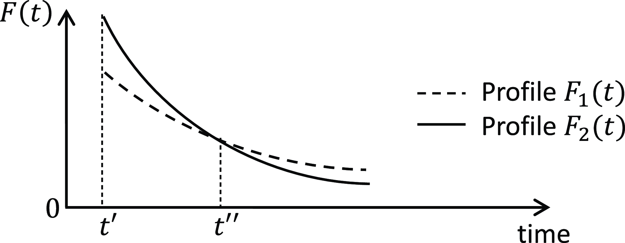
has a direct effect on short-term carbon emissions. The elementary result is the following. Consider two trajectories for the economy, labeled as 1 and 2. Assume that
 $g_{F_{2} }(t)\lt g_{F_{1}}(t)$
(resp.
 $g_{F_{2}}(t)\gt g_{F_{1}}(t)$
)
 $\forall t\in \lbrack t^{\ast },+\infty)$
. Then, following the time profile
 $F_{2}(.)$
instead of
 $F_{1}(.)$
means accelerating (resp. slowing) carbon emissions. In other words, short-term carbon emissions are higher (resp. lower) in profile
 $2$
than in profile
 $1,$
in the sense that there exists a date
 $\tilde {t}\gt t^{\ast }$
such that
 $F_{2}(t)\gt F_{1}(t)$
(resp.
 $F_{2}(t)\lt F_{1}(t)$
)
 $,$
 $\forall t\in \lbrack t^{\ast },\tilde {t}[$
. Thus, if the technology shock yields
 $g_{F_{2}}(t)\lt g_{F_{1}}(t)$
for all
 $t$
, this means that it increases (resp. decreases) early carbon emissions.
2.4 Representative household and basic constraints
The instantaneous utility function of the representative infinitely-lived household depends on both consumption,
 $C(t)$
, and the stock of carbon,
 $Z(t)$
.Footnote
12
The intertemporal utility function is given by:
 \begin{equation} U=\int _{0}^{+\infty }\left [ \ln \big (C(t)\big)-\omega \left [ Z(t)\right] \right] e^{-\rho t}\,dt,\text{ }\rho \gt 0\text{ and }\omega \geq 0\text{.} \end{equation}
 $\omega \left [ Z(t)\right]$
is the instantaneous disutility of the stock of carbon at date
 $t$
, with
 $d\omega \left [ Z(t)\right] /dZ(t)\gt 0$
.
 $\rho$
is the rate of time preferences.Footnote
13
At each date, a constant flow
 $L\gt 0$
of skilled labor is used by the two competing R&D sectors. Normalizing
 $L$
to unity, we have
 \begin{equation} \int _{0}^{1}L_{ri}(t)\,di+\int _{0}^{1}L_{fi}(t)\,di=1,\ \forall t\geq 0. \end{equation}
In this model, there is no explicit inclusion of unskilled labor in the production of final goods (including resource production). We make this modeling choice to keep the model tractable, allowing us to obtain closed-form solutions, and analyze the transition outside the steady state. Consequently, our study does not feature a research-production trade-off, a recurring characteristic in models with DTC models with climate considerations (see, for example, Casey, Reference Casey2024 or Hassler et al. Reference Hassler, Krusell and Olovsson2022). Nevertheless, we maintain an analytical framework that enables us to focus on our main objective: studying the impact of technological shocks on the direction of technical progress as well as on the carbon emissions path.
Last, the final good produced at each date
 $t\geq 0$
is either used for consumption or the production of renewable and fossil-related intermediate goods:
 \begin{equation} Y(t)=C(t)+\int _{0}^{1}y_{ri}(t)di+\int _{0}^{1}y_{fi}(t)di,\ \forall t\geq 0\text{.} \end{equation}
3. Behavior of agents
As is usual, we choose the final good as the numeraire good; its price is normalized to unity. In the rest of the paper,
 $p_{ji}(t)$
,
 $p_{R}(t)$
,
 $p_{F}(t)$
will respectively denote the price of the intermediate good
 $i\in \lbrack 0,1]$
used in sector
 $j=r,f$
, the price of the clean renewable resource and the price of the fossil resource. Finally,
 $w(t)$
is the wage rate, and
 $\bar {r}(t)$
is the rate of interest.
3.1 Final good sector
The final sector maximizes the following profit function:
 \begin{align} \pi _{Y}(t) & =\left [ Y_{r}(t)^{(\varepsilon -1)/\varepsilon }+Y_{f} (t)^{(\varepsilon -1)/\varepsilon }\right] ^{\varepsilon /(\varepsilon -1)}\nonumber \\ &\quad -\sum \limits _{j=r,f}\int _{0}^{1}p_{ji}(t)x_{ji}(t)\,di-p_{R}(t)R-p_{F} (t)F(t). \end{align}
The first-order conditions for the choice of input
 $F(t)$
and of the quantities
 $x_{ri}(t)$
and
 $x_{fi}(t)$
of renewable and fossil-related intermediate goods are:
 \begin{align} p_{F}(t) & =(1-\alpha)Y(t)^{1/\varepsilon }Y_{f}(t)^{(\varepsilon -1)/\varepsilon }/F(t)\equiv MP_{F}(t). \end{align}
 \begin{align} p_{ri}(t) & =\alpha Y(t)^{1/\varepsilon }Y_{r}(t)^{-1/\varepsilon }\left [ \frac {RA_{ri}(t)}{x_{ri}(t)}\right] ^{1-\alpha }\equiv MP_{x_{ri}} (t)\text{,} \end{align}
 \begin{align} p_{fi}(t) & =\alpha Y(t)^{1/\varepsilon }Y_{f}(t)^{-1/\varepsilon }\left [ \frac {F(t)A_{fi}(t)}{x_{fi}(t)}\right] ^{1-\alpha }\equiv MP_{x_{fi} }(t)\text{. } \end{align}
Each condition equates the input price to its marginal productivity and gives the production sector’s inverse demand for this input.
3.2 Intermediate goods sectors
We assume that, at each date
 $t\geq 0$
, all intermediate goods
 $x_{ji}(t)$
,
 $j=r,f$
,
 $i\in \lbrack 0,1]$
, are monopolistically supplied. By Equation (7), producing a quantity
 $x_{ji}(t)$
of intermediate good requires an amount
 $\psi x_{ji}(t)$
of final good. The profit derived from this activity thus writes
 \begin{equation} \pi _{ji}(t)=x_{ji}(t)\left [ p_{ji}(t)-\psi \right], \end{equation}
where
 $p_{ji}(t)$
is given by (14) and (15). In this context, monopoly prices
 $p_{ji}(t)$
exhibit a mark-up above the marginal cost
 $\psi$
:
 \begin{equation} p_{ji}(t)=\frac {\psi }{\alpha },\ \forall j=r,f,\ \forall i\in \lbrack 0,1]. \end{equation}
They are time-invariant, as well as independent of the sector
 $j=r,f$
to which they are dedicated and of the type of intermediate good
 $i\in \lbrack 0,1]$
, as is standard.
3.3 R&D sectors
In Acemoglu et al. (Reference Acemoglu, Aghion, Bursztyn and Hemous2012), where time is modeled as discrete, the innovator achieves a monopoly position that lasts for the shortest time interval in their analytical framework: one period. We adapt this assumption by considering that the monopoly position endures for a duration
 $dt$
. Specifically, when an innovation—generating a new, more productive type of intermediate good
 $x_{ji}(t)$
, with
 $j=r,f$
, and
 $i\in (0,1)-$
occurs at time
 $t\geq 0$
, the innovator benefits exclusively from the profit
 $\pi _{ji}(t)dt$
obtained from the sale of the new intermediate good over the interval
 $(t,t+dt)$
. This assumption of an infinitesimal patent length is a theoretical simplification that allows us to derive tractable results in both steady-state and transitional dynamics.Footnote
14
In the real world, it approximates industries characterized by rapid technological obsolescence or high competition, where firms can expect only brief periods of market exclusivity before competitors enter or new technologies emerge—such as technology or software, where the lifecycle of innovations is short. Thus, the value of an innovation at date
 $t$
—and therefore the value of the associated patent—is equal to the flows of profits earned over the period
 $(t,t+dt)$
. We have:
 \begin{equation} V_{ji}(t)=\pi _{ji}(t)dt, \end{equation}
where it follows from the analysis of the previous section (Equation (16) with equilibrium price (17)) that
 $\pi _{ji}(t)$
can be expressed as a linear function of
 $x_{ji}(t)$
only:
 \begin{equation} \pi _{ji}(t)=\frac {(1-\alpha)\psi }{\alpha }x_{ji}(t). \end{equation}
We know that at each date
 $t\geq 0$
,
 $L_{ji}(t)$
scientists are dedicated to improving the quality level of intermediate good
 $i\in \lbrack 0,1]$
used in sector
 $j=r,f$
, each having the instantaneous probability
 $\eta _{j} L_{ji}(t)^{\beta }$
of being the successful innovator. For any
 $j=r,f$
, and any
 $i\in \lbrack 0,1]$
, the total profit from R&D activities thus writes
 \begin{equation} \pi _{R\&Dji}(t)=\eta _{j}L_{ji}(t)^{\beta }V_{ji}(t)-w(t)L_{ji} (t), \end{equation}
where
 $V_{ji}(t)$
is given by Equation (18).
Maximizing this profit leads to the first-order condition
 $\beta \eta _{j} L_{ji}(t)^{\beta -1}V_{ji}(t)=w(t),$
which implies
 \begin{equation} \eta _{r}L_{ri}(t)^{\beta -1}V_{ri}(t)=\eta _{f}L_{fi}(t)^{\beta -1} V_{fi}(t)\text{.} \end{equation}
This equation simply means that the equilibrium marginal productivity of scientists is equalized everywhere they are allocated.
 $V_{ji}(t)$
is obtained from (18) and (19):
 \begin{equation} V_{ji}(t)=\frac {\psi (1-\alpha)}{\alpha }x_{ji}(t)dt. \end{equation}
As in the literature, the value of an innovation depends on two effects (see Acemoglu, Reference Acemoglu2002). First, the price effect, represented by the term
 $\frac {\psi (1-\alpha)}{\alpha }$
, which depends on both the production cost of the intermediate good (see Equation (7)) and parameter
 $\alpha$
, which characterizes the inverse demand function of this good (see Equations (14) and (15)). Second, the market size effect, that is, the quantity of the intermediate good
 $x_{ji}(t)$
sold.
From Equations (14), (15) and (17), we have
 $x_{ri}(t)=x_{r}(t)$
and
 $x_{fi} (t)=x_{f}(t),\forall i\in \lbrack 0,1].$
Then, from Equations (19) and (22), we also have
 $\pi _{ji}(t)=\pi _{j}(t)=\frac {(1-\alpha)\psi }{\alpha }x_{j}(t)$
and
 $V_{ji} (t)=V_{j}(t)=\pi _{j}(t)dt,\forall$
 $j=r,f$
 $,$
and
 $\forall$
 $i\in \lbrack 0,1].$
Consequently, the first-order condition
 $\beta \eta _{j} L_{ji}(t)^{\beta -1}V_{j}(t)=w(t)$
implies
 $L_{ji}(t)=$
 $L_{j}(t),\forall j=r,f,$
and
 $\forall i\in \lbrack 0,1].$
Since the ratio of intermediate-good uses, i.e., the relative market size,
 $x_{r}(t)/x_{f}(t)$
plays a central role in the following analysis, we will henceforth use the compact notation
 \begin{equation*} \frac {x_{r}(t)}{x_{f}(t)}\equiv X(t). \end{equation*}
We observe here that the relative value of innovations is equal to the relative market size:
 $V_{r}(t)/V_{f}(t)=\pi _{r}(t)/\pi _{f} (t)=X(t)$
(see Equation (22)). The relative price effect does not appear in this equation because we have assumed that the production cost of intermediate goods is identical in both sectors and that the demand functions for these two types of goods from the final sector have the same price elasticity.
Furthermore, we have:
 \begin{equation} \left [ \frac {L_{r}(t)}{L_{f}(t)}\right] ^{1-\beta }=\frac {\eta _{r}x_{r} (t)}{\eta _{f}x_{f}(t)}\equiv \frac {\eta _{r}}{\eta _{f}} X(t). \end{equation}
This equation highlights that the direction of technical change, i.e., the relative effort in R&D, is determined by the relative market size,
 $X(t)$
. The interpretation is the following. An increase in the ratio of intermediate goods’ uses,
 $x_{r}(t)/x_{f}(t)\equiv X(t)$
, raises the relative profitability of the production of intermediate goods in the renewable-based sector (see Equation (19)). Research in the renewable-oriented sector thus becomes more profitable (see Equation (18)). As a result, renewable-oriented research drains relatively more labor:
 $L_{r}(t)/L_{f}(t)$
increases. This means, for example, that an increase in the use of wind turbines (for instance, due to a subsidy), while the use of coal-fired power plants remains fixed or decreases, reallocates the overall research effort in favor of renewable-oriented innovation.
Using Equations (10) and (23), we have:
 \begin{equation} L_{r}\left [ X(t)\right] =\frac {1}{\left [ \frac {\eta _{r}}{\eta _{f} }X(t)\right] ^{\frac {1}{\beta -1}}+1}. \end{equation}
Observe that
 $d\left [ L_{r}(X(t))\right] /d\left [ X(t)\right] \gt 0$
:
 $L_{r}(t)$
is an increasing function of
 $X(t)$
with an upper bound equal to
 $1$
. Equation (23) showed that the relative effort in renewable-oriented R&D,
 $L_{r}(t)/L_{f}(t)$
, is an increasing function of the intermediate goods ratio
 $X(t)$
. Since the total amount of labor in R&D in the economy is fixed, the total effort devoted to renewable-oriented R&D is also increasing with
 $X(t)$
.
With the earlier-made assumption that quality levels
 $A_{ji}(0)$
are initially equal across intermediates
 $i\in \lbrack 0,1]$
for each sector
 $j=r,f$
, the law of motion (6) implies that the quality levels
 $A_{ji}(t)$
in the symmetric equilibrium obey the same average dynamics within the renewable and fossil-oriented sectors. We have
 $A_{ji}(t)=A_{j} (t)$
,
 $j=r,f$
and
 $i\in \lbrack 0,1]$
. Thus Equation (6) writes:
 \begin{equation} \dot {A}_{j}(t)=\gamma \eta _{j}L_{j}(t)A_{j}(t),\ \forall j=r,f. \end{equation}
Finally, Equations (6) and (10) yield:
 \begin{equation} g_{A_{r}/A_{f}}\left [ X(t)\right] =\gamma \eta _{r}\left [ L_{r}\left [ X(t)\right] \right] -\gamma \eta _{f}\left [ 1-L_{r}\left [ X(t)\right] \right] \text{,} \end{equation}
where
 $L_{r}\left [ X(t)\right]$
is given by Equation (24).
Observe that the growth rate of the knowledge ratio
 $g_{A_{r}/A_{f}}\left [ X(t)\right]$
, that is, the direction of technical change (see, e.g., Acemoglu, Reference Acemoglu2002), is an increasing function of the effort in renewable-oriented R&D. From Equation (24), we can deduce that the direction of technical change is also an increasing function of the ratio of intermediate goods
 $X(t)$
. In other words, by making renewable-oriented R&D relatively more profitable, an increase in
 $X(t)$
draws labor from fossil-oriented research and reallocates it to renewable-oriented R&D; as a consequence, fossil-related knowledge
 $A_{f}(t)$
grows less fast and renewable-related knowledge
 $A_{r}(t)$
grows faster.
3.4 Resource sector
On the competitive natural resource market, we assume extraction costs to be nil. The maximization of the profit function
 $\int _{t}^{+\infty }p_{F}(s)F(s)e^{-\int _{t}^{s}\bar {r}(u)du}ds$
, subject to
 $\dot {S}(s)=-F(s)$
,
 $S(s)\geq 0$
,
 $F(s)\geq 0,$
 $s\geq t$
, yields the standard decentralized equilibrium “Hotelling rule” (Hotelling, Reference Hotelling1931):
 \begin{equation} g_{p_{_{F}}}(t)=\bar {r}(t)\text{ for all }t\text{.} \end{equation}
As usual, the transversality condition is
 $\lim _{t\rightarrow +\infty }S(t)=0$
.
Remark Extraction costs typically increase as the resource becomes scarcer while technical progress reduces them. Our simplifying assumption, which is standard in the growth literature, implicitly assumes that the two effects compensate for each other. A simple way to introduce extraction costs in this type of model would be to use the approach formulated by André and Smulders (Reference André and Smulders2014). At each date
 $t$
, the flow
 $-\dot {S}(t)$
is extracted, and a proportion
 $F(t)=-\dot {S}(t)/(1+\mu (t))$
,
 $\mu (t)\gt 0$
, is supplied to the market, while
 $-\dot {S}(t)\mu (t)/(1+\mu (t))$
is lost. Here,
 $\mu (t)/(1+\mu (t))$
represents the extraction unit cost in terms of the resource. We define
 $\hat {\mu }(t)$
as the term
 $\dot {\mu }(t)/(1+\mu (t))$
. If
 $\hat {\mu }(t)\lt 0$
, the unit cost of extraction declines over time due to technical progress that increases exploration efficiency. Conversely,
 $\hat {\mu } (t)$
may be positive, reflecting the increasing inaccessibility of reserves. Under these conditions, profit maximization yields
 $g_{p_{F}}(t)=\bar {r}(t)+\hat {\mu }(t)$
. Thus,
 $g_{p_{F}}(t)$
could be either positive or negative (the latter occurring if extraction costs decrease sufficiently rapidly). In this case one can show that, except for the resource price, neither the steady-state dynamics nor the non-steady-state dynamics of the economy change.
3.5 Representative household
The household’s consumption-saving arbitrage determines the growth rate of consumption
 $C(t)$
. The maximization of the intertemporal utility function (9), subject to any intertemporal budget constraint arising under a perfect financial market, yields the standard Ramsey-Keynes condition:
 $g_{C}(t)=\bar {r}(t)-\rho.$
In Appendix C, we show that consumption is a linear function of output, from which we deduce:
 \begin{equation} g_{C}(t)=g_{Y}(t)=\bar {r}(t)-\rho. \end{equation}
4. Equilibrium and dynamics of the decentralized economy
In Subsection 4.1, we characterize the dynamics of resource use and the dynamics of the intermediate-good ratio, the latter being central to the characterization of the equilibrium of the decentralized economy. In Subsection 4.2, we compute this equilibrium and analyze the resulting dynamics of the economy.
4.1 Dynamics of carbon emissions and the intermediate-good ratio
Lemma 1 presents two key results. First, it expresses the dynamics of carbon emissions
 $F(t)$
by relating their growth rate to the growth rate of the intermediate-good ratio,
 $X(t)$
. Second, it provides the differential equation that governs the dynamics of
 $X(t)$
.
Lemma 1.
The growth rate of carbon emissions
 $g_{F}(t)$
is a function of the level of the intermediate-good ratio
 $X(t)$
and of its growth rate
 $gX(t)$
:
 \begin{equation} g_{F}(t)=-\rho -\frac {X(t)}{1+X(t)}g_{(Y_{r}/Y_{f})^{\frac {\varepsilon -1}{\varepsilon }}}(t)=-\rho -\frac {X(t)}{1+X(t)}g_{X}(t)\text{.} \end{equation}
The differential equation that allows to study the dynamics of the intermediate-good ratio
 $X(t)$
is the following:
 \begin{align} g_{X}\left [ X(t)\right] & =\frac {1-\alpha }{\frac {\varepsilon } {\varepsilon -1}-\frac {\alpha +X(t)}{1+X(t)}}\left [ \rho +g_{A_{r}/A_{f}}\left [ X(t)\right] \right], \end{align}
with
 $g_{A_{r}/A_{f}}\left [ X(t)\right]$
given by Equation (
26
).
Proof. See Appendix D.
Let us briefly comment on the dynamics of
 $X(t)$
, which are characterized by Equation (30) and graphically illustrated in the phase diagram in Figure 1. The properties of this equation depend on the substitutability of the two sectors, that is, the value of parameter
 $\varepsilon$
.Footnote
15
Phase diagram in the cases
 $\varepsilon \gt 1$
and
 $\varepsilon \lt 1$
.

If
 $\varepsilon \gt 1$
, we show in Appendix D.3 (Case A) that function
 $g_{X}(.)$
is an increasing function of
 $X(t)$
with a negative lower bound and a positive upper bound (see Figure 1). This implies that there exists an interior steady-state level
 $X_{SS}\gt 0$
such that
 $g_{X}(X_{SS})=0$
. Since
 $g_{X}\left [ X(t)\right] \gt 0$
for all
 $X(t)\gt X_{SS}$
and
 $g_{X}\left [ X(t)\right] \lt 0$
for all
 $X(t)\lt X_{SS}$
, this steady state is unstable. If
 $X(t)\lt X_{SS}$
,
 $X(t)$
decreases down to
 $0.$
If
 $X(t)\gt X_{SS}$
,
 $X(t)$
increases indefinitely.
If
 $\varepsilon \lt 1$
, we show in Appendix D.3 (Case B) that
 $g_{X}(.)$
is a decreasing function of
 $X(t)$
with a negative lower bound and a positive upper bound (see Figure 1). Thus, there exists
 $X_{SS}$
such that
 $g_{X}(X_{SS})=0$
. Here, since
 $g_{X}\left [ X(t)\right] \lt 0$
for all
 $X(t)\gt X_{SS}$
and
 $g_{X}\left [ X(t)\right] \gt 0$
for all
 $X(t)\lt X_{SS}$
, this steady state is stable.
In the two cases (
 $\varepsilon \gt 1$
and
 $\varepsilon \lt 1$
), the common interior steady state
 $X_{SS}\gt 0$
is thus such that
 $g_{A_{r}/A_{f}}(X_{SS})=-\rho$
(see Equation (30)). Then,
 $X_{SS}$
is an implicit solution of
 $g_{A_{r}/A_{f}}(X_{SS})=-\rho$
and Equation (24)
 $.$
Since
 $g_{X}(X_{SS})=0$
, from Equation (29), we also have
 $g_{F}(t)=-\rho$
in the steady state.
In Appendix D.3, we provide further comments on the dynamics of
 $X(t)$
. We analyze the overall (steady-state and non-steady-state) dynamics of the economy below in Subsection 4.2.
4.2 General equilibrium: definition and characterization
Before analyzing the impact of technology shocks, we first provide a definition and a characterization of the general equilibrium of the decentralized economy. In particular, we show that the entire dynamics of the economy are essentially determined by the dynamics of
 $X$
.
Definition 1.
An equilibrium of the decentralized economy consists of the time paths of quantities
 $\left \{ Y(t),C(t),x_{r}(t),x_{f}(t),F(t),L_{r} (t),L_{f}(t),A_{r}(t),A_{f}(t)\right \} _{t=0}^{\infty }$
and prices
 $\left \{ p_{R}(t), p_{f}(t),p_{F}(t),\bar {r}(t),w(t)\right \} _{t=0}^{\infty }$
such that: the representative household maximizes her utility; firms maximize their profits; the final good market, the labor market, the resource market, and the financial good market are perfectly competitive and clear; each innovator receives the profit instantaneously derived from the sale of the intermediate good associated with her innovation.
We now sum up the characterization of the general equilibrium in the following lemma.
Lemma 2. The equilibrium of the decentralized economy is characterized as follows.
1. The dynamics of variables
 $X(t)$
,
 $F(t)$
,
 $L_{r}(t)$
,
 $A_{r}(t)$
and
 $A_{f}(t)$
are given by Equations (
30
), (
29
), (
24
) and (
25
) respectively.
2. In the interior steady state, equilibrium quantities, growth rates, and prices are given by:
a) quantities and growth rates
 \begin{align*} L_{r} & =\frac {\gamma \eta _{f}-\rho }{\gamma (\eta _{r}+\eta _{f})},\text{ } L_{f}=\frac {\gamma \eta _{r}+\rho }{\gamma (\eta _{r}+\eta _{f})},\text{ }F(t)=F(0)e^{-\rho t},\text{ }C(t)=(1-\alpha {{}^2})Y(t),\\ x_{r}(t) & =\frac {\alpha {{}^2} Y(t)}{\psi (1+H)},\text{ }x_{f}(t)=\frac {\alpha {{}^2} Y(t)}{\psi (1+1/H)},\text{ }X_{SS}\equiv \frac {x_{r}(t)}{x_{f}(t)}=\frac {1} {H},\text{ where }H=\frac {\eta _{r}}{\eta _{f}}\left ( \frac {L_{f}}{L_{r} }\right) ^{1-\beta },\\ \frac {A_{r}(t)}{A_{f}(t)} & =\frac {F(t)}{R}X_{SS}^{\frac {\varepsilon (1-\alpha)+\alpha }{(1-\alpha)(\varepsilon -1)}},\text{ }g_{A_{r}/A_{f} }(t)=g_{F}(t)=-\rho \text{,}\\ g_{Y} & =g_{C}=g_{Y_{r}}=g_{Y_{f}}=g_{x_{r}}=g_{x_{f}}=g_{A_{r}}=\gamma \eta _{r}L_{r},\text{ and }g_{A_{f}}=\gamma \eta _{f}L_{f}=\gamma \eta _{r} L_{r}+\rho. \end{align*}
b) prices
 \begin{align*} & p_{j}=\frac {\psi }{\alpha },\text{ for }j=r,f,\text{ }p_{F}(t)=p_{F} (0)e^{\bar {r}t},\text{ }\bar {r}=\gamma \eta _{r}L_{r}+\rho,\\ & \text{ and }w(t)=\frac {\beta \psi (1-\alpha)\eta _{j}}{\alpha }L_{j}^{\beta -1}x_{j}(t),\text{ for }j=r,f. \end{align*}
If
 $\varepsilon \gt 1$
, this steady state is unstable. If
 $\varepsilon \lt 1$
, it is stable.
Proof. The computation of the interior steady-state equilibrium of the decentralized economy is presented in Appendix E.
We now provide a more detailed analysis of the dynamics of the economy, as presented in Lemma2.
4.2.1 Steady-state dynamics
Parameter
 $\varepsilon$
has no impact on the equilibrium variables (levels and growth rates of the quantities and prices) in the steady state. The two research sectors are simultaneously active: as explained in Subsection 2.2, this comes from the assumption that the instantaneous probability that scientists produce an innovation at date
 $t$
is a strictly concave function of the number of scientists (see Equation (4)). Consequently, the two stocks of knowledge,
 $A_{r}(t)$
and
 $A_{f}(t)$
increase over time. Furthermore, since
 $A_{r}(t)/A_{f}(t)$
is an increasing linear function of
 $F(t)$
, we have
 $g_{A_{r}/A_{f}}(t)=g_{F}(t)=-\rho$
.
Observe that, in the steady state, both the renewable-energy intensity of output,
 $R/Y(t)$
, and the carbon intensity of output,
 $F(t)/Y(t)$
, are decreasing over time. Indeed,
 $g_{R}(t)-g_{Y}(t)=$
 $-g_{Y}(t)=-\gamma \eta _{r}L_{r}\lt 0$
and
 $g_{F}(t)-g_{Y}(t)=$
 $-\rho -(\bar {r}-\rho)=-\gamma \eta _{r}L_{r}-\rho \lt 0$
. Note that these results are consistent with stylized facts as those presented in, e.g., Casey (Reference Casey2024).
We can also observe that the expenditure shares of renewable energy,
 $p_{R}(t)R/Y(t)$
, and of fossil energy,
 $p_{F}(t)F(t)/Y(t)$
, are constant over time in the steady state. If we assume that renewable energy is produced competitively from non-skilled labor,
 $R=\xi L_{R}$
, then
 $g_{p_{R}} (t)=g_{w}(t)=g_{Y}(t)$
. That is why
 $p_{R}(t)R/Y(t)$
is constant. Similarly, one has
 $g_{p_{F}}(t)=\bar {r}$
,
 $g_{F}(t)=-\rho$
and
 $g_{Y}(t)=\bar {r}-\rho$
; therefore,
 $p_{F}(t)F(t)/Y(t)$
is constant too.
4.2.2 Non-steady-state dynamics
Here also, the two research sectors are simultaneously active (except in the two corner solutions—see the phase diagram (Figure 1)). Now, parameter
 $\varepsilon$
plays a crucial role.
First, let us analyze the dynamics of the key variables. In the case
 $\varepsilon \gt 1$
, suppose that
 $X(t)\lt X_{SS}$
(R&D is initially fossil-oriented). We know that, in this case, we have
 $g_{X}(t)\lt 0$
:
 $X(t)$
decreases over time and tends toward zero. This implies that
 $g_{L_{r}/L_{f} }(t)\lt 0$
and
 $g_{A_{r}/A_{f}}\lt -\rho$
, for any
 $t$
: R&D becoming gradually more and more fossil-oriented, the economy is in a fossil-oriented trap—this case of steady-state instability is central to the analysis of Acemoglu et al. (Reference Acemoglu, Aghion, Bursztyn and Hemous2012). If
 $X(t)\gt X_{SS}$
(R&D is initially renewable-oriented), we have symmetrical results; in particular,
 $g_{X}(t)\gt 0$
and
 $g_{L_{r}/L_{f}}(t)\gt 0$
for any
 $t$
: R&D is gradually becoming more and more renewable-oriented. In the case
 $\varepsilon \lt 1$
, if
 $X(t)\lt X_{SS}$
, we have
 $g_{X}(t)\gt 0$
:
 $X(t)$
increases over time and tends to the steady state. That implies that
 $g_{L_{r}/L_{f}}(t)\gt 0$
for any
 $t$
: R&D is gradually becoming more and more renewable-oriented. If
 $X(t)\gt X_{SS}$
,
 $g_{X}(t)$
is negative, and therefore
 $X(t)$
tends to the steady state also.
Second, let us explain why the interior steady state is unstable if
 $\varepsilon \gt 1$
, and stable if
 $\varepsilon \lt 1$
. Assume
 $X(t)\gt X_{SS}$
. This means that R&D is initially renewable-oriented, that is, the labor ratio in R&D,
 $L_{r}/L_{f}$
, is large. Formally, we have
 $L_{r}(t)/L_{f} (t)\gt (\gamma \eta _{f}-\rho)/(\gamma \eta _{r}+\rho)$
(see Lemma2). Therefore, the growth rate of the knowledge ratio,
 $g_{A_{r}/A_{f}}$
, is also large: one has
 $g_{A_{r}/A_{f}}(t)\gt -\rho$
. In the absence of any variation of other(s) variable(s), the ratio of the marginal productivities of intermediate goods,
 $g_{MPx_{r}/MPx_{f}}(t)$
, increases (resp. decreases) if
 $\varepsilon \gt 1$
(resp.
 $\varepsilon \lt 1$
). Since this ratio must remain equal to
 $1$
,
 $X(t)$
increases (resp. decreases) if
 $\varepsilon \gt 1$
(resp.
 $\varepsilon \lt 1$
). Assume now
 $X(t)\lt X_{SS}$
, the result is symmetric:
 $X(t)$
decreases (resp. increases) if
 $\varepsilon \gt 1$
(resp.
 $\varepsilon \lt 1$
). That explains why the interior steady state is unstable (resp. stable) if
 $\varepsilon \gt 1$
(resp.
 $\varepsilon \lt 1$
).
5. Climate impact of a technology shock
As exposed in Subsection 2.2, we assume that an exogenous technology shock occurs at date
 $t^{\ast }\gt 0$
. This shock makes
 $A_{r}(t)$
and
 $A_{f}(t)$
both (discontinuously) jump upward at this date. If the shock is green, the knowledge ratio
 $A_{r}(t)/A_{f}(t)$
also jumps upwards; if the shock is gray, the ratio jumps downwards.Footnote
16
We consider two trajectories for the economy. In the first one, labeled as 1, there is no technology shock. In the second, labeled as 2, the technology shock changes the ratio
 $A_{r}/A_{f}$
at date
 $t^{\ast }$
. Hence for all
 $t\lt t^{\ast }$
, we have
 $A_{r2}(t)/A_{f2}(t)=A_{r1}(t)/A_{f1}(t)$
and, at date
 $t^{\ast }$
,
 $A_{r2}(t^{\ast })/A_{f2}(t^{\ast })\gt A_{r1}(t^{\ast })/A_{f1}(t^{\ast })$
in the case of a green shock, and
 $A_{r2}(t^{\ast })/A_{f2}(t^{\ast })\lt A_{r1}(t^{\ast })/A_{f1}(t^{\ast })$
in the case of a gray shock. To analyze the climate impact of the shock, we need to compare carbon emissions in trajectory 1 and trajectory 2 for
 $t\gt t^{\ast }$
.
The main results of the paper (presented in Propositions 1 and 2 below) are formally demonstrated in Appendix F.
As we want to study how the shock affects the time path of carbon emissions, and thus of fossil resource use,
 $F$
, a central variable is the anticipated growth rate of the marginal productivity of the resource:
 $g_{MP_{F}}$
. For instance, if firms anticipate that the resource becomes less profitable tomorrow (i.e., in the long term) than today (i.e., in the short term), they use it more today and less tomorrow.Footnote
17
In Appendix D.1, we have shown that
 $MP_{F} (t)=(1-\alpha)\frac {Y(t)}{F(t)}\frac {1}{X(t)+1}.$
By differentiating this equation with respect to time, we obtain the following equation, which shows that the relationship between the dynamics of
 $MP_{F}$
and the dynamics of
 $F$
depends on the dynamics of
 $X(t)$
:
 \begin{equation} g_{MP_{F}}(t)=g_{Y}(t)-g_{F}(t)-\frac {X(t)}{1+X(t)}g_{X}(t)\text{,} \end{equation}
where
 $g_{Y}(t)=\bar {r}(t)-\rho$
(see Equation (28)). For a given interest rate
 $\bar {r}(t)$
, the dynamics of the marginal productivity of the resource depend on the term
 $\left [ X(t)/(1+X(t))\right] g_{X}(t)$
, and thus notably on the dynamics of
 $X(t)$
, characterized by
 $g_{X}(t)$
.
As we will show, the transmission channel through which the technological shock modifies the trajectory of the economy, and, in particular, short-term emissions, is the same regardless of the value of
 $\varepsilon$
. The main steps of this common transmission channel are the following:
-
• impact of the shock on the ratio of intermediate-good marginal productivities,
 $MP_{x_{r}}/MP_{x_{f}}$
and the ratio of intermediate goods
$X$
at date
$t^{\ast }$
,
-
• reallocation of research efforts due to the modification of
$X$
, -
• impact of this reallocation on the dynamics of the knowledge stock ratio
$A_{r}/A_{f}$
for
$t\gt t^{\ast }$
, -
• impact on the dynamics of the marginal productivity of the fossil resource
$MP_{F}$
for
$t\gt t^{\ast }$
, -
• impact on the intertemporal resource use profile and, therefore, particularly on short-term emissions.


5.1
The renewable and fossil-based production sectors are gross complements:
$\varepsilon \lt 1$

In the case where the renewable and fossil-based production sectors are gross complements (
 $\varepsilon \lt 1$
), a technology shock at date
 $t$
has an impact on short-term carbon emissions that is presented in Proposition 1 below.
Proposition 1.
When the renewable and fossil-based production sectors are gross complements (
 $\varepsilon \lt 1$
), a green (resp. gray) technology shock, i.e., a discontinuous increase (resp. decrease) in the knowledge ratio
 $A_{r}/A_{f}$
, increases (resp. decreases) short-term carbon emissions (that is, emissions occurring right after the shock
Footnote
18
).
Proof. See Appendix F.
All formal elements regarding this case are presented in Appendix F. Here, we identify the transmission channel between the technological shock and its climate impact and we provide the main intuitions that are required to interpret the results. For simplicity, we focus on the case of a green technology shock.
As
 $\varepsilon \lt 1$
, the steady state
 $X_{SS}$
is stable (see Lemma2). We thus assume that the initial state of the economy is
 $X_{1}(t^{\ast })=X_{SS}$
. First, recall that before the technology shock, the ratio of intermediate-good marginal productivities,
 $MP_{x_{r}}/MP_{x_{f}}$
, is equal to one. At the date
 $t^{\ast }$
of the shock (where
 $A_{r}/A_{f}$
increases),
 $MP_{x_{r}}/MP_{x_{f}}$
gets lower since
 $\varepsilon \lt 1$
(see Equation (D.4)). Then, firms reduce
 $X$
to restore the equality of this ratio to one; we have
 $X_{2}(t^{\ast })\lt X_{1}(t^{\ast })$
. We know that the two R&D sectors are financed by profits made on the sales of intermediate goods. Therefore, the change in
 $X$
has a direct effect on this financing: it causes a reallocation of labor between the two sectors of research. That is the basis of the dynamics impacts of the green technology shock that we now examine. Formally, the decrease in
 $X$
induces a reduction of
 $L_{r}/L_{f}$
(see Equation (23)), that is, labor in renewable-oriented R&D is reduced, which promotes fossil-oriented R&D. This result is analogous to the reduction in energy efficiency R&D observed in Casey (Reference Casey2024) in his study of the rebound effect.
The last steps concern the impact of these instantaneous modifications on the dynamics of variables
 $X$
,
 $MP_{F}$
, and
 $F$
. For
 $t\gt t^{\ast }$
, the reduction of
 $L_{r}/L_{f}$
leads to a decrease in the growth rate of the knowledge stock ratio,
 $A_{r}/A_{f}$
: formally, we have
 $g_{A_{r}/A_{f}}(t)\lt -\rho$
—see Equation (26). Hence, this modifies the dynamics of
 $X$
(see Equation (30)):
 $g_{X_{2}}(t)$
is positive (the economy is on the left side of the phase diagram). This also changes the dynamics of
 $MP_{F}$
(see Equation (31)). In trajectory 1 (i.e., in steady state), we have
 $g_{MP_{F1}}(t)=\bar {r} (t)-\rho -g_{F1}(t)$
(since
 $g_{X1}(t)=0$
). In trajectory 2, we have
 $g_{MP_{F2}}(t)=\bar {r}(t)-\rho -g_{F2}(t)-\frac {X_{2}(t)}{1+X_{2}(t)} g_{X2}(t)$
. Assume that, as a first step, firms in the final sector do not modify the dynamics of the resource (i.e.,
 $g_{F2}(t)=g_{F1}(t)$
for any
 $t\gt t^{\ast }$
). Since
 $g_{X2}(t)$
is positive, we have
 $g_{MP_{F2} }(t)\lt g_{MP_{F1}}(t)$
, for any
 $t\gt t^{\ast }$
. Thus, after the shock, firms anticipate that the resource becomes less profitable tomorrow (i.e., in the long term) than today (i.e., in the short term); they thus decide to use more resource today and less tomorrow. In other words, the growth rate of resource use (and hence the growth rate of carbon emissions),
 $g_{F}(t)$
, gets lower at any date
 $t$
(see Equation (29)). This is why short-term carbon emissions increase.
5.2
The renewable and fossil-based production sectors are gross substitutes:
$\varepsilon \gt 1$

In the case where the renewable and fossil-based production sectors are gross substitutes (
 $\varepsilon \gt 1$
), a technology shock at date
 $t^{\ast }$
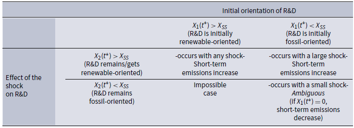
has an impact on short-term carbon emissions that is presented in Proposition 2 below and summarized in Table 1.
Impact of a green technology shock on short-term carbon emissions when
 $\varepsilon \gt 1$

Proposition 2.
When the renewable and fossil-based production sectors are gross substitutes (
 $\varepsilon \gt 1$
), the impact of a green technology shock on short-term carbon emissions is the following:
—if the shock yields
 $X_{2}(t^{\ast })\gt X_{SS}$
, short-term emissions are increased (whatever the initial orientation of R&D,
 $X_{1}(t^{\ast })$
),
—if the shock yields
 $X_{2}(t^{\ast })\lt X_{SS}$
(that is, if
 $X_{1}(t^{\ast })\lt X_{SS}$
and the shock is relatively small), short-term emissions can be increased or reduced. In the particular case where
 $X_{1}(t^{\ast })=0$
, short-term emissions are reduced.
The results are reversed in the case of a gray shock.
Proof. See Appendix F.
Here also, we focus on the case of a green technology shock.
We know that, at the date
 $t^{\ast }$
of the shock (where
 $A_{r}/A_{f}$
increases), the ratio
 $MP_{x_{r}}/MP_{x_{f}}$
gets higher (the reasoning presented in the previous subsection goes in opposite ways since
 $\varepsilon \gt 1$
). In this case,
 $X$
jumps up:
 $X_{2}(t^{\ast })\gt X_{1}(t^{\ast })$
.
The interior steady state being unstable since
 $\varepsilon \gt 1$
, two initial situations are possible, as shown in Subsection 4.2: either
 $X_{SS} \lt X_{1}(t^{\ast })$
(pre-shock R&D is renewable-oriented) or
 $X_{1}(t^{\ast })\lt X_{SS}$
(pre-shock R&D is fossil-oriented). In the first case (
 $X_{SS}\lt X_{1}(t^{\ast })$
), we necessarily have
 $X_{ss}\lt X_{1}(t^{\ast })\lt X_{2}(t^{\ast })$
after the shock. In the second case (
 $X_{1}(t^{\ast })\lt X_{SS}$
), we can have either
 $X_{1}(t^{\ast })\lt X_{ss}\lt X_{2}(t^{\ast })$
, that is, the shock makes R&D renewable-oriented, or
 $X_{1}(t^{\ast })\lt X_{2} (t^{\ast })\lt X_{ss}$
, that is, the shock is not sufficient and leaves R&D fossil-oriented. We now analyze the dynamics of the economy by distinguishing between the two cases that can occur after the shock.
5.2.1 Post-shock R&D remains/gets renewable-oriented (
$X_{2}(t^{\ast })\gt X_{ss}$
)

As explained above, this situation can occur in two cases. In the first, pre-shock R&D is renewable-oriented:
 $X_{ss}\lt X_{1}(t^{\ast })$
. This case occurs if the knowledge-stock ratio is initially high; formally, if
 $A_{r1}(t^{\ast })/A_{f1}(t^{\ast })\gt (F_{1}(t^{\ast })/R)X_{SS}^{\frac {\varepsilon (1-\alpha)+\alpha }{(1-\alpha)(\varepsilon -1)}}$
. Here, whatever the size of the shock, we have
 $X_{ss}\lt X_{1}(t)\lt X_{2}(t)$
and
 $0\lt g_{X1} (t)\lt g_{X2}(t)$
, for
 $t\gt t^{\ast }$
(the economy is on the right side of the phase diagram in Figure 1, and the steady state is unstable).Footnote
19
In the second case, pre-shock R&D is fossil-oriented:
 $X_{1}(t^{\ast })\lt X_{ss}$
. This case occurs if the knowledge-stock ratio is initially low: if
 $A_{r1}(t^{\ast })/A_{f1}(t^{\ast })\lt (F_{1}(t^{\ast })/R)X_{SS}^{\frac {\varepsilon (1-\alpha)+\alpha }{(1-\alpha)(\varepsilon -1)}}$
. So, for any
 $t\gt t^{\ast }$
,
 $X_{1}(t)$
decreases over time (the economy is now on the left side of the phase diagram). Absent any technology stock, the economy would converge toward a fossil-oriented trap. Assuming here that
 $X_{1}(t^{\ast })\lt X_{ss} \lt X_{2}(t^{\ast })$
means that the technology shock is large enough to switch from a fossil-oriented situation (
 $X\lt X_{ss}$
) to a renewable-oriented situation (
 $X_{ss}\lt X$
); formally, we have
 $A_{r2}(t^{\ast })/A_{f2}(t^{\ast })\gt (F_{2}(t^{\ast })/R)X_{SS}^{\frac {\varepsilon (1-\alpha)+\alpha } {(1-\alpha)(\varepsilon -1)}}$
. Finally, in this case, we have
 $g_{X1} (t)\lt 0\lt g_{X2}(t)$
for any
 $t\gt t^{\ast }$
.
We can now understand why short-term emissions increase following the shock. We need to go back to Equation (31). As in Subsection 5.1, we assume that, as a first step, firms in the final sector do not modify the dynamics of the resource (i.e.,
 $g_{F2}(t)=g_{F1}(t)$
for any
 $t\gt t^{\ast }$
). So, we have
 $g_{MP_{F2}}(t)\lt g_{MP_{F1}}(t)$
, for any
 $t\gt t^{\ast }$
, in the two cases studied here. Indeed, in the first case, where
 $X_{ss}\lt X_{1}(t)\lt X_{2}(t)$
and
 $0\lt g_{X1}(t)\lt g_{X2}(t)$
, for
 $t\gt t^{\ast }$
, we have
 $\frac {X_{1}(t)}{1+X_{1}(t)}g_{X1}(t)\lt \frac {X_{2}(t)}{1+X_{2}(t)} g_{X2}(t)$
, which explains the result. In the second case, the result is immediate since we have
 $g_{X1}(t)\lt 0\lt g_{X2}(t)$
, for all
 $t\gt t^{\ast }$
.
So, as in the case
 $\varepsilon \lt 1$
, the shock makes the fossil resource less profitable tomorrow than today, which explains why the final sector decides to use more resource in the short term and less in the long term. Formally, we have
 $g_{F2}(t)\lt g_{F1}(t)$
at any date
 $t\gt t^{\ast }$
, which implies that
 $F$
increases at date
 $t=t^{\ast }$
:
 $F_{2}(t^{\ast })\gt F_{1}(t^{\ast })$
.
This result may seem paradoxical. First, as mentioned above, it is contrary to the initial intuition. Specifically, since the two production subsectors—renewable and fossil-based—are gross substitutes, the fossil resource becomes relatively less productive in the short term; one might expect this to lead to a decrease in carbon emissions. Second, the post-shock economy is increasingly renewable-oriented (in terms of R&D). However, carbon emissions are increased in the short term.
5.2.2 Post-shock R&D remains fossil-oriented (
$X_{2}(t^{\ast })\lt X_{ss}$
)

This case can occur only if pre-shock R&D is fossil-oriented:
 $0\leq X_{1}(t^{\ast })\lt X_{ss}$
. As stated in Table 1, the results are generally ambiguous in this case. However, if we assume that the initial situation is
 $X_{1}(t^{\ast })=0$
(and thus
 $L_{r}(t^{\ast })=0$
)—that is, the economy is in a fossil-oriented trap, we obtain non-ambiguous results. We thus focus here on the case where
 $X_{1}(t^{\ast })=0\lt X_{2}(t^{\ast })\lt X_{ss}$
, which means that the shock is relatively small (formally,
 $A_{r2}(t^{\ast })/A_{f2} (t^{\ast })\lt (F_{2}(t^{\ast })/R)X_{SS}^{\frac {\varepsilon (1-\alpha)+\alpha }{(1-\alpha)(\varepsilon -1)}}$
). Here, for any
 $t\gt t^{\ast }$
, one has
 $g_{X2}(t)\lt 0$
: the economy is increasingly relying on the fossil sector.Footnote
20
In this case, the ratio of knowledge stocks
 $A_{r}/A_{f}$
is small, and it leads to a progressive decrease in
 $X$
over time; formally, we have
 $g_{A_{r}/A_{f}}(t)\lt -\rho$
. Since
 $X_{1}(t)=0$
and
 $g_{X2}(t)\lt 0$
, if, once again, we first assume that
 $g_{F2}(t)=g_{F1}(t)$
, we have
 $g_{MP_{F2}}(t)\gt g_{MP_{F1}}(t)$
, for any
 $t\gt t^{\ast }$
: we are now in a situation where the resource becomes more profitable tomorrow than today. That is why carbon emissions get lower in the short term.
Even though, in a certain sense, this result does not contradict the initial intuition that carbon emissions decrease because the resource becomes less productive in the short term, it remains paradoxical. We are indeed facing a case where the economy is increasingly fossil-oriented, yet carbon emissions decrease in the short term.
5.3
The production technology of output is Cobb-Douglas:
$\varepsilon =1$

The result (short-term emissions are not modified) is demonstrated in Appendix F.
The essential point is that at the date
 $t^{\ast }$
of the shock, the marginal productivities of the renewable and fossil-related intermediate goods are affected similarly. That implies that the ratio of intermediate-good marginal productivities,
 $MP_{xr}/MP_{xf}$
, and therefore the variable
 $X$
, are unchanged; formally, we have
 $MP_{xr}(t)/MP_{xf}(t)=X(t)=1$
, and thus
 $g_{X}(t)=0$
, for all
 $t\gt t^{\ast }$
(see Equations (D.1) and (D.2)).
For
 $t\gt t^{\ast }$
, since
 $X$
is unchanged, there is no reallocation of labor in R&D: formally,
 $L_{r}/L_{f}$
is not modified. Therefore, the knowledge-stock ratio
 $A_{r}/A_{f}$
is at a higher level, but its dynamics, characterized by the rate of growth
 $g_{A_{r}/A_{f}}$
, are unchanged.
Finally, since the dynamics of
 $X$
are not affected, the dynamics of the marginal productivity of the resource,
 $g_{MP_{F}}$
, are also unchanged. That is why there is no change in the rate of resource extraction over time and, therefore, no change in short-term emissions. Formally, in Equation (31), we have
 $g_{X}(t)=0$
,
 $g_{F}(t)=-\rho$
, and thus
 $g_{MP_{F}}(t)=\bar {r}(t)$
.
In summary, the green technological shock (i.e., the increase in
 $A_{r}/A_{f}$
) leads to an increase in the levels of
 $Y$
(see Equation (1)),
 $C$
,
 $x_{r}$
and
 $x_{f}$
(see Appendix C), but it does not affect the dynamics of these variables. It also does not affect the dynamic use of fossil resource, implying that short-term carbon emissions are unchanged.
6. Conclusion
Green technology improvements, i.e., improvements in the productivity of low-carbon activities, are widely regarded as essential for achieving climate neutrality. These improvements may manifest as technology shocks. The primary objective of this study is to analyze the dynamic general-equilibrium effects of such shocks. In the context of a (fully) endogenous growth model with directed technical change and a fossil resource, we have explored the intertemporal reallocations induced by (green and gray) technology shocks, with a particular emphasis on the time profile of carbon emissions.
As technology shocks affect research sectors and the dynamics of knowledge accumulation, their impacts can be non-intuitive and thus warrant careful analysis. In particular, we have demonstrated how the reallocations in the (renewable and fossil-oriented) R&D efforts induced by such shocks alter the entire dynamics of the economy, notably the time profile of the marginal productivity of the fossil resource. As a result, firms intertemporally reallocate their use of this fossil resource, which consequently alters the timing of their carbon emissions.
Basically, three elements drive the results: the substitutability between renewable and fossil-based production subsectors, the state of the economy before the shock, and the magnitude of the shock. First, assume first gross complementarity between the two subsectors. In this case, a green technology shock (one that is (relatively) oriented towards renewable technologies) leads to an increase in short-term carbon emissions (emissions occurring immediately after the shock). Now, consider gross substitutability between the two subsectors. If the post-shock economy is renewable-oriented (i.e., if R&D becomes more and more renewable-oriented), regardless of its initial state, short-term emissions also rise. In contrast, if the economy is fossil-oriented before the shock and remains so even after the shock (for example, with a relatively small shock), the impact of a green technology shock on short-term emissions is ambiguous; we show, however, that if there was renewable-oriented research activity before the shock, the shock reduces short-term emissions. These results are reversed in the case of a gray (oriented towards fossil-related technologies) technology shock.
These dynamics highlight the crucial role of energy efficiency R&D in directing the trajectory of technical progress and determining the path of carbon emissions. Our findings emphasize that the technological shock has opposing effects on the allocation of research efforts depending on whether the production subsectors are substitutes or complements. However, in most cases, its overall impact on fossil resource use and carbon emissions remains independent of this substitutability.
Note that all the mechanisms studied here occur outside the interior steady state. In the case of gross substitutability, this is indeed straightforward since the steady state is unstable. Here, the trajectories we analyze progressively diverge from the steady state. In the case of gross complementarity, we assume that, prior to the shock, the economy is in the interior steady state, as it is stable. By modifying the two knowledge stocks, that are state variables, the shock causes the economy to deviate from this steady state. Since the steady state is stable, all quantities, prices, and growth rates follow trajectories that progressively converge back toward it.
Future lines of research may include, for example, relaxing the assumption of a Hotellian fossil resource—i.e., endogenizing the stock of available fossil fuel and, consequently, the amount of potentially emitted carbon. Other avenues could involve employing a semi-endogenous growth model, considering distinct elasticities of output with respect to production factors in each subsector, or, following Lemoine (Reference Lemoine2024), using a constant elasticity of substitution function for energy production.
Acknowledgments
The authors would like to thank the anonymous Associate Editor and the two anonymous referees for their helpful comments and suggestions. André Grimaud acknowledges funding from ANR under grant ANR-17-URE-0010 (Investissements d’Avenir program).
APPENDICES
A. Proof of equation (6) and generalization
Recall that
 $A_{ji}(t)$
is the quality level of sector
 $j$
’s intermediate good
 $i$
, with
 $j=r,f,$
and
 $i\in \lbrack 0,1]$
. The number of scientists dedicated to improving this quality level is
 $L_{ji}(t)$
.
Starting from date
 $t\geq 0$
, consider an infinitesimal time duration
 $dt\gt 0$
that will be assumed to tend to
 $0$
. Here, we examine the evolution of the quality level
 $A_{ji}(t)$
over the time interval
 $[t,t+dt]$
. This interval being close to
 $0$
, it is clear that the probability that there is strictly more than one innovation in sector
 $j$
relative to the intermediate good
 $i$
becomes negligible. One can thus restrict the analysis to two possibilities.
The first possibility is that there is one innovation in sector
 $j$
for the intermediate good
 $i$
over the interval
 $[t,t+dt]$
. This occurs with the instantaneous probability given in Equation (4), multiplied by the time duration
 $dt$
:
 $\eta _{j}L_{ji}(t)^{\beta }dt$
. In this case, according to Equation (5), the quality level after the
 $dt$
period of time is
 $A_{ji}(t+dt)=A_{ji}(t)+\gamma A_{ji}(t)L_{ji}(t)^{\sigma }$
.
The second possibility is that there is no innovation in sector
 $j$
for intermediate good
 $i$
over the interval
 $[t,t+dt]$
. The probability that there is more than one innovation being negligible, the possibility of
 $0$
innovation is given by the complementary probability
 $1-\eta _{j} L_{ji}(t)^{\beta }dt$
. In that case, the quality level after the
 $dt$
period of time remains
 $A_{ji}(t+dt)=A_{ji}(t)$
.
It follows that the expected value of
 $A_{ji}(t)$
at a date
 $t+dt$
that is sufficiently close to
 $t$
can be expressed as
 $E[A_{ji}(t+dt)]=[A_{ji} (t)+\gamma A_{ji}(t)L_{ji}(t)^{\sigma }]\eta _{j}L_{ji}(t)^{\beta } dt+A_{ji}(t)[1-\eta _{j}L_{ji}(t)^{\beta }dt]$
. After simplifying, we obtain
 \begin{equation*} E[A_{ji}(t+dt)]=A_{ji}(t)+\gamma \eta _{j}L_{ji}(t)^{\beta +\sigma }A_{ji}(t)dt, \end{equation*}
which gives the following expression of the expected increase of
 $A_{ji}$
over the infinitesimal time interval
 $[t,t+dt]$
:
 \begin{equation*} \frac {E[A_{ji}(t+dt)]-A_{ji}(t)}{dt}=\gamma \eta _{j}L_{ji}(t)^{\beta +\sigma }A_{ji}(t). \end{equation*}
As
 $dt$
tends to
 $0$
, the latter formula gives the expected instantaneous rise in
 $A_{ji}(t)$
at date
 $t$
, denoted in the text by
 \begin{equation*} \dot {A}_{ji(t)}\equiv \underset {dt\rightarrow 0}{\lim }\frac {E[A_{ji} (t+dt)]-A_{ji}(t)}{dt}. \end{equation*}
Its expression in Equation (6) is immediately obtained.
This methodology can be used to obtain a more general law of motion. Suppose that the probability of producing an innovation is given by the function
 $\eta _{j}[L_{ji}(t),A_{ji}(t)]$
, and that the jump in quality is given by the function
 $\gamma \lbrack L_{ji}(t),A_{ji}(t)]$
, where functions
 $\eta _{j}[.,.]$
and
 $\gamma \lbrack.,.]$
are both increasing with respect to
 $L_{ji}(t)$
and
 $A_{ji}(t)$
. By using the same proof as above, one obtains the law of motion
 $\dot {A}_{ji(t)}=\eta _{j}[L_{ji}(t),A_{ji}(t)]\gamma \lbrack L_{ji}(t),A_{ji}(t)]$
. This law is rather general and encompasses most of the ones used in the literature, as illustrated in the two following examples.
a. Assume
 $\eta _{j}[L_{ji}(t),A_{ji}(t)]=\eta _{j}L_{ji}(t)^{\beta }$
,
 $\eta _{j}\gt 0$
,
 $0\leq \beta \leq 1$
, and
 $\gamma \lbrack L_{ji}(t),A_{ji}(t)]=\gamma A_{ji}(t)^{\varphi }$
,
 $\gamma \gt 0$
,
 $\varphi \leq 1$
. One gets
 $\dot {A} _{ji(t)}=\gamma \eta _{j}L_{ji}(t)^{\beta }A_{ji}(t)^{\varphi }$
. This law, which considers decreasing returns in the stock of knowledge, is formally identical to those assumed in the semi-endogenous growth literature, as for instance in Jones (Reference Jones1999).
b. Assume
 $\eta _{j}[L_{ji}(t),A_{ji}(t)]=\eta _{j}L_{ji}(t)$
,
 $\eta _{j}\gt 0$
, and
 $\gamma \lbrack L_{ji}(t),A_{ji}(t)]=\max [A_{ji}(t),i\in (0,1)]\equiv A_{j}(t)^{\max }$
. One gets
 $\dot {A}_{ji(t)}=\eta _{j}L_{ji}(t)A_{j}(t)^{\max }$
. This law is similar to the one initially introduced in Aghion and Howitt (Reference Aghion and Howitt1992).
B. Dynamics of the fossil resource and climate
Here, we show how a modification of the growth rate of carbon emissions
 $g_{F}(t)$
affects climate. We assume that, after a certain date
 $t^{\prime }$
, there exist two trajectories for the economy, labeled as 1 and 2. These trajectories are such that
 $\int _{t^{\prime }}^{+\infty }F_{1}(t)dt=\int _{t\prime }^{+\infty }F_{2}(t)dt=S(t^{\prime }).$
Assume that
 $g_{F_{2} }(t)\lt g_{F_{1}}(t),$
 $\forall t\in \lbrack t^{\prime },+\infty)$
—see Figure 2. Assume that
 $g_{F_{2}}(t)\lt g_{F_{1}}(t),$
 $\forall t\in \lbrack t^{\prime },+\infty)$
. Then, following the time profile
 $F_{2}(.)$
instead of
 $F_{1}(.)$
means accelerating carbon emissions. In other words, short-term carbon emissions are higher in profile
 $2$
than in profile
 $1,$
in the sense that there exists a date
 $t^{\prime \prime }\gt t^{\prime }$
such that
 $F_{2} (t)\gt F_{1}(t),$
 $\forall t\in \lbrack t^{\prime },t^{\prime \prime }[$
.
Time paths of carbon emissions.

The proof is as follows. Observe first that there exists one date
 $t^{\prime \prime }$
such that
 $F_{2}(t^{\prime \prime })=F_{1}(t^{\prime \prime })$
—see Figure 2. If
 $t^{\prime \prime }$
did not exist, that would mean that either
 $F_{2}(t)\lt F_{1}(t)$
or
 $F_{1}(t)\lt F_{2}(t)$
for all
 $t\in \lbrack t^{\prime },+\infty)$
, which is incompatible with the equality
 $\int _{t^{\prime }}^{+\infty }F_{1}(t)dt=\int _{t^{\prime }}^{+\infty }F_{2}(t)dt.$
The inequality
 $\dot {F}_{2}(t)/F_{2}(t)\lt \dot {F}_{1}(t)/F_{1}(t)$
is equivalent to
 $d\log F_{2}(t)/dt\lt d\log F_{1}(t)/dt$
for all
 $t$
. Consider two given dates:
 $t$
and
 $t+h,$
 $h\gt 0$
. Then, we have
 $\int _{t}^{t+h}\left [ d\log F_{2}(x)/dx\right] dx\lt \int _{t}^{t+h}\left [ d\log F_{1}(x)/dx\right] dx$
, and thus
 $\log F_{2}(t+h)-\log F_{2}(t)\lt \log F_{1}(t+h)-\log F_{1}(t).$
We now consider
 $t+h\equiv t^{\prime \prime }$
such that
 $\log F_{2}(t+h)=\log F_{1}(t+h)$
—we have established at the beginning of this proof that such a date exists. Then the above inequality becomes
 $\log F_{2}(t)\gt \log F_{1}(t),$
 $\forall t\in \lbrack t^{\prime },t^{\prime \prime }[$
, that is
 $F_{2} (t)\gt F_{1}(t),$
 $\forall t\in \lbrack t^{\prime },t^{\prime \prime }[$
.
In Section 5, we consider two trajectories for the economy. In the first one, labeled as 1, there is no technology shock. In the second, labeled as 2, the economy benefits from a technology shock at date
 $t^{\ast }$
. This appendix allows us to state that if
 $g_{F_{2}}(t)\lt g_{F_{1}}(t)$
(resp.
 $g_{F_{2} }(t)\gt g_{F_{1}}(t)$
)
 $\forall t\in \lbrack t^{\ast },+\infty)$
, the technology shock increases (resp. decreases) early carbon emissions. In other words, a change in the expected dynamics of
 $F(t)$
has a direct effect on short-term carbon emissions.
C. Proof of Equation (28)
Taking Equation (11), substituting
 $y_{ji}(t)=\psi x_{ji}(t)$
from Equation (7), and making use of the notations
 $x_{r}(t)=x_{ri}(t)$
and
 $x_{f}(t)=x_{fi}(t)$
, for all
 $i\in \lbrack 0,1]$
(from Subsection 3.3), one obtains the following relation:
 \begin{equation} C(t)=Y(t)-\psi \left [ x_{r}(t)+x_{f}(t)\right]. \end{equation}
By substituting the price
 $p_{ji}(t)=\psi /\alpha$
from Equation (17) into Equations (14) and (15), we get:
 $\alpha Y(t)^{1/\varepsilon }Y_{r}(t)^{(\varepsilon -1)/\varepsilon }=\left ( \psi /\alpha \right) x_{r}(t)$
and
 $\alpha Y(t)^{1/\varepsilon }Y_{f} (t)^{(\varepsilon -1)/\varepsilon }=\left ( \psi /\alpha \right) x_{f}(t)$
. Thus, one deduces
 $\psi \left [ x_{r}(t)+x_{f}(t)\right] /\alpha =\alpha Y(t)^{1/\varepsilon }\left [ Y_{r}(t)^{(\varepsilon -1)/\varepsilon } +Y_{f}(t)^{(\varepsilon -1)/\varepsilon }\right]$
. Finally, we have
 $\psi \left [ x_{r}(t)+x_{f}(t)\right] /Y(t)=\alpha {{}^2} Y(t)^{1/\varepsilon }\left [ Y_{r}(t)^{(\varepsilon -1)/\varepsilon } +Y_{f}(t)^{(\varepsilon -1)/\varepsilon }\right] /Y(t)=\alpha {{}^2}$
. We can now plug this last expression into Equation (C.1), and obtain
 $C(t)=Y(t)(1-\alpha ^{2})$
, which implies that the growth rates of the two variables are identical in any equilibrium.
D. Proof of Lemma1
D.1 Computation of
$g_{F}(t)$

The relationship between the growth rate of the fossil resource,
 $g_{F}(t)$
, and the growth rate of the intermediate-good ratio,
 $g_{X}(t)$
, is the direct consequence of the three first-order conditions of the profit-maximization of the final sector (Equations (13), (14) and (15)).
First, since
 $x_{ri}(t)=x_{r}(t)$
and
 $A_{ri}(t)=A_{r}(t)$
for all
 $i=0,1$
, Equations (14) and (2) become
 $p_{ri}(t)=\alpha \left [ \frac {Y(t)}{Y_{r}(t)}\right] ^{1/\varepsilon }\left [ \frac {RA_{R} (t)}{x_{r}(t)}\right] ^{1-\alpha }$
and
 $Y_{r}(t)=R^{1-\alpha }A_{r} (t)^{1-\alpha }x_{r}(t)^{\alpha }$
. We can deduce
 $p_{ri}(t)=\left [ \alpha Y(t)^{1/\varepsilon }Y_{r}(t)^{\frac {\varepsilon -1}{\varepsilon }}\right] /x_{r}(t)\equiv MP_{x_{r}}(t)$
. Similarly, using the symmetry condition and Equation (3), Equation (15) becomes
 $p_{fi} (t)=\left [ \alpha Y(t)^{\frac {1}{\varepsilon }}Y_{f}(t)^{\frac {\varepsilon -1}{\varepsilon }}\right] /x_{f}(t)\equiv MP_{x_{f}}(t)$
. These two results imply
 \begin{equation} \frac {MP_{x_{r}}(t)}{MP_{x_{f}}(t)}=\left [ \frac {Y_{r}(t)}{Y_{f}(t)}\right] ^{\frac {\varepsilon -1}{\varepsilon }}\frac {1}{X(t)}. \end{equation}
By using (17), we have
 $MP_{x_{r}}(t)/MP_{x_{f}}(t)=1$
, and therefore
 \begin{equation} X(t)=\left [ \frac {Y_{r}(t)}{Y_{f}(t)}\right] ^{\frac {\varepsilon -1}{\varepsilon }}\text{ and }g_{X}(t)=\frac {\varepsilon -1}{\varepsilon }g_{Y_{r}/Y_{f}}(t). \end{equation}
Second, consider Condition (13) relative to the fossil resource. It can be rewritten
 $p_{F}(t)=(1-\alpha)\frac {Y(t)}{F(t)}\left [ \frac {Y_{f} (t)}{Y(t)}\right] ^{\frac {\varepsilon -1}{\varepsilon }}$
. Equation (1) can also be rewritten as
 $Y(t)=Y_{f} (t)\left [ \left ( \frac {Y_{r}(t)}{Y_{f}(t)}\right) ^{\frac {\varepsilon -1}{\varepsilon }}+1\right] ^{\frac {\varepsilon }{\varepsilon -1}}$
, which gives
 $\left [ \frac {Y_{f}(t)}{Y(t)}\right] ^{\frac {\varepsilon -1}{\varepsilon } }=\frac {1}{\left [ \frac {Y_{r}(t)}{Y_{f}(t)}\right] ^{\frac {\varepsilon -1}{\varepsilon }}+1}$
.
Third, by mixing these results with Equation (D.2), we obtain:
 \begin{equation} p_{F}(t)=(1-\alpha)\frac {Y(t)}{F(t)}\frac {1}{\left [ \frac {Y_{r}(t)}{Y_{f} (t)}\right] ^{\frac {\varepsilon -1}{\varepsilon }}+1}=(1-\alpha)\frac {Y(t)}{F(t)}\frac {1}{X(t)+1}\equiv MP_{F}(t)\text{.} \end{equation}
By log-differentiating Equation (D.3) with respect to time, we have
 $g_{p_{F}}(t)=g_{Y}(t)-g_{F}(t)+g_{\frac {1}{X+1}}(t)$
. The term
 $g_{\frac {1}{X+1}}(t)$
is equal to
 $\frac {-X(t)}{1+X(t)}g_{X}(t)$
. Then, by replacing
 $g_{p_{F}}(t)$
and
 $g_{Y}(t)$
by their expressions in Equations (27) and (28) we obtain Equation (29):
 $g_{F}(t)=-\rho -\frac {X(t)}{1+X(t)}g_{(Y_{r}/Y_{f})^{\frac {\varepsilon -1}{\varepsilon }}}(t)=-\rho -\frac {X(t)}{1+X(t)}g_{X}(t)$
.
First, Equation (29) shows that the growth rate of carbon emissions
 $g_{F}(t)$
is a decreasing function of the psychological discount rate,
 $\rho$
. As usual in growth models, an increase in
 $\rho$
holds back the growth of output and consumption (see Equation (28)). Consequently, the marginal productivity of the fossil resource grows less fast:
 $g_{MP_{F}}(t)$
is reduced at any date
 $t$
(see Equation (D.3)). Therefore, as explained above, the final sector uses the resource more today and less in the future:
 $g_{F}(t)$
is lower at any date
 $t$
.
Second, Equation (29) also shows that
 $g_{F}(t)$
diminishes when the growth rate of the intermediate-good ratio,
 $g_{X}(t)$
, increases (in other words, when
 $x_{r}(t)/x_{f}(t)$
grows faster). Indeed, a higher
 $g_{X}(t)$
means that intermediate good
 $x_{r}(t)$
becomes relatively less profitable than
 $x_{f}(t)$
. Without a change in any other variable(s), this would reduce the growth rate of the ratio of marginal productivities of intermediate goods,
 $g_{MP_{xr}/MP_{xf}}(t)$
(see Equation (D.1)). However, we know that intermediate goods must have the same productivity, which implies
 $g_{MP_{xr}/MP_{xf}}(t)=0$
at any date
 $t$
; this is only possible if
 $\left [ (\varepsilon -1)/\varepsilon \right] g_{Yr/Yf}(t)$
increases (see Equations (D.1) and (D.2)). The only variable available to firms that can hold the equality between the productivities of intermediate goods equal is the flow of fossil resource
 $F(t)$
(see Equations (2) and (3)). We have shown above how the changes in the dynamics of
 $F(t)$
are determined by changes in the dynamics of its productivity
 $MP_{F}(t)$
. From Equation (D.3), we see that if
 $\left [ (\varepsilon -1)/\varepsilon \right] g_{Yr/Yf}(t)$
increases, then
 $g_{F}(t)$
decreases. So, here, too, the final sector uses the resource more today and less tomorrow:
 $g_{F}(t)$
is lower at any date
 $t$
.
In summary, when
 $g_{X}(t)$
gets higher, the final sector accelerates the use of the resource over time (
 $g_{F}(t)$
is lower at any date
 $t$
). This simultaneously allows it to maintain the marginal productivities of intermediate goods equal and to optimally respond to the decline in the growth of the resource productivity over time.
D.2 Computation of
$g_{X}(t)$

Now, we aim to obtain a differential equation that allows fully characterizing the dynamics of
 $X(t)$
.
By using Equations (2) and (3), the ratio of marginal productivities of the intermediate goods given by Equation (D.1) becomes
 \begin{equation} \frac {MP_{x_{r}}(t)}{MP_{x_{f}}(t)}=\left [ \frac {R}{F(t)}\right] ^{\frac {(1-\alpha)(\varepsilon -1)}{\varepsilon }}\left [ \frac {A_{r}(t)} {A_{f}(t)}\right] ^{\frac {(1-\alpha)(\varepsilon -1)}{\varepsilon }} X(t)^{\frac {\varepsilon (\alpha -1)-\alpha }{\varepsilon }}. \end{equation}
We know that this ratio is equal to
 $1$
. Then, by log-differentiating the expression with respect to time and by replacing
 $g_{F}(t)$
by its expression given in Equation (29), we obtain
 $\frac {(1-\alpha)(\varepsilon -1)}{\varepsilon }\rho +\left [ \frac {(1-\alpha)(\varepsilon -1)X(t)} {\varepsilon (1+X(t))}+\frac {\varepsilon (\alpha -1)-\alpha }{\varepsilon }\right] g_{X}(t)+\frac {(1-\alpha)(\varepsilon -1)}{\varepsilon }g_{A_{r}/A_{f}}(t)=0$
. By dividing both sides of the equation by
 $\left [ \frac {(1-\alpha)(\varepsilon -1)X(t)}{\varepsilon (1+X(t))}+\frac {\varepsilon (\alpha -1)-\alpha }{\varepsilon }\right]$
(which can be simplified to
 $-\frac {X(t)+\alpha -\varepsilon (\alpha -1)}{\varepsilon (1+X(t))}$
), and by rearranging, we obtain differential equation (30) given in Lemma1, which characterizes the dynamics of
 $X(t)$
:
 $g_{X}\left [ X(t)\right] =\frac {1-\alpha }{\frac {\varepsilon }{\varepsilon -1}-\frac {\alpha +X(t)}{1+X(t)} }\left [ \rho +g_{A_{r}/A_{f}}\left [ X(t)\right] \right],$
with
 $g_{A_{r}/A_{f}}\left [ X(t)\right]$
given by Equation (26).
D.3 Dynamics of
$X(t)$

Case A: The renewable and fossil-based sectors are gross substitutes:
$\varepsilon \gt 1$

If
 $\varepsilon \gt 1$
, the denominator of the right-hand-side of Equation (30),
 $\frac {\varepsilon }{\varepsilon -1}-\frac {\alpha +X(t)}{1+X(t)}$
, is strictly positive. This expression is a decreasing function of
 $X(t)$
that takes its values from
 $\frac {\varepsilon }{\varepsilon -1}-\alpha$
(when
 $X(t)$
tends to
 $0$
) to
 $\frac {\varepsilon }{\varepsilon -1}-1$
(when
 $X(t)$
tends to infinity). Then, the growth rate of
 $X(t)$
,
 $g_{X}\left [ X(t)\right]$
, is an increasing function of
 $X(t)$
that takes its values from
 $\frac {(1-\alpha)(\rho -\gamma \eta _{f})}{\frac {\varepsilon }{\varepsilon -1}-\alpha }$
(when
 $X(t)$
tends to
 $0$
) to
 $\frac {(1-\alpha)(\rho +\gamma \eta _{r})}{\frac {\varepsilon }{\varepsilon -1}-1}$
(when
 $X(t)$
tends to infinity).Footnote
21
First, note that the latter bound is unambiguously positive. We assume now that
 $\rho -\gamma \eta _{f}\lt 0$
. This assumption, common in growth theory, means that the psychological discount rate is not too high as compared to the exogenous parameters characterizing the efficiency of the fossil-oriented research sector. Consequently, the minimum threshold of
 $g_{X}\left [ X(t)\right]$
is negative, which implies that there exists a steady-state level
 $X_{SS}\gt 0$
such that
 $g_{X}(X_{SS})=0$
. Since
 $g_{X}\left [ X(t)\right] \gt 0$
for all
 $X(t)\gt X_{SS}$
and
 $g_{X}\left [ X(t)\right] \lt 0$
for all
 $X(t)\lt X_{SS}$
, this steady state is unstable. If
 $X(t)\lt X_{SS}$
,
 $X(t)$
decreases down to
 $0$
, and the economy reaches another steady state, which is stable since
 $g_{X}(0)\lt 0$
. If
 $X(t)\gt X_{SS}$
,
 $X(t)$
increases indefinitely.
Case B: The renewable and fossil-based sectors are gross complements:
$\varepsilon \lt 1$

If
 $\varepsilon \lt 1$
, the denominator in Equation (30),
 $\frac {\varepsilon }{\varepsilon -1}-\frac {\alpha +X(t)}{1+X(t)}$
is strictly negative. It is a decreasing function of
 $X(t)$
that takes its values from
 $\frac {\varepsilon } {\varepsilon -1}-\alpha$
(when
 $X(t)$
tends to
 $0$
) to
 $\frac {\varepsilon }{\varepsilon -1}-1$
(when
 $X(t)$
tends to infinity). Then,
 $g_{X}\left [ X(t)\right]$
is an decreasing function of
 $X(t)$
that takes its values from
 $\frac {(1-\alpha)(\rho -\gamma \eta _{f})}{\frac {\varepsilon }{\varepsilon -1}-\alpha }$
(when
 $X(t)$
tends to
 $0$
) to
 $\frac {(1-\alpha)(\rho +\gamma \eta _{r})}{\frac {\varepsilon }{\varepsilon -1}-1}$
(when
 $X(t)$
tends to infinity).Footnote
22
As in the case
 $\varepsilon \gt 1$
, we assume that
 $\rho -\gamma \eta _{f}\lt 0$
. The upper bound of
 $g_{X}$
is thus positive while its lower bound is negative. Thus, there exists
 $X_{SS}$
such that
 $g_{X}(X_{SS})=0$
. Here, since
 $g_{X}\left [ X(t)\right] \lt 0$
for all
 $X(t)\gt X_{SS}$
and
 $g_{X}\left [ X(t)\right] \gt 0$
for all
 $X(t)\lt X_{SS}$
, this steady state is stable.
E. Characterization of the steady-state equilibrium of the decentralized economy
1. Computation of
 $L_{r}$
and
 $L_{f}$
From Equation (30), we have
 $\rho +g_{A_{r}/A_{f}}(X_{SS})=0$
. From Equation (26), we have
 $g_{A_{r}/A_{f}}(X_{SS})=\gamma \eta _{r}L_{r}-\gamma \eta _{f}(1-L_{r})$
. One thus deduces
 $L_{r}=\frac {\gamma \eta _{f}-\rho }{\gamma (\eta _{r}+\eta _{f})}$
and
 $L_{f}=\frac {\gamma \eta _{r}+\rho }{\gamma (\eta _{r}+\eta _{f})}$
.
2. Computation of
 $X_{SS}$
From Equation (23), and the expressions of
 $L_{r}$
and
 $L_{f}$
obtained above, we have
 $X_{SS}=\frac {\eta _{f}}{\eta _{r} }\left ( \frac {L_{r}}{L_{f}}\right) ^{1-\beta }=\frac {\eta _{f}}{\eta _{r} }\left ( \frac {\gamma \eta _{f}+\rho }{\gamma \eta _{r}+\rho }\right) ^{1-\beta }=\frac {1}{H}$
.
3. Computation of
 $x_{r}(t)$
and
 $x_{f}(t)$
In Appendix C, we have obtained
 $C(t)=(1-\alpha {{}^2})Y(t)$
. Then, by using Equation (11) and Equation (7), we get:
 $Y(t)=(1-\alpha {{}^2})Y(t)+x_{r}(t)+x_{f}(t)$
. Since
 $X_{SS}\equiv \frac {x_{r}(t)}{x_{f}(t)} =\frac {1}{H}$
, we obtain
 $x_{r}(t)=\frac {\alpha {{}^2} Y(t)}{\psi (1+H)}$
and
 $x_{f}(t)=\frac {\alpha {{}^2} Y(t)}{\psi (1+1/H)}$
.
4. Computation of
 $A_{r}(t)/A_{f}(t)$
From Equation (D.4), we have
 $\frac {A_{r}(t)}{A_{f} (t)}=\frac {F(t)}{R}X_{SS}^{\frac {\varepsilon (1-\alpha)+\alpha }{(1-\alpha)(\varepsilon -1)}}$
.
5. Computation of the rates of growth
We start by computing the general relation between growth rates.
Equation (1) gives:
 $Y(t)=\left [ Y_{r} (t)^{\frac {\varepsilon -1}{\varepsilon }}+Y_{f}(t)^{\frac {\varepsilon -1}{\varepsilon }}\right] ^{\frac {\varepsilon }{\varepsilon -1}}=Y_{f}(t)\left [ \left ( \frac {Y_{r}(t)}{Y_{f}(t)}\right) ^{\frac {\varepsilon -1}{\varepsilon } }+1\right] ^{\frac {\varepsilon }{\varepsilon -1}}.$
Equation (D.2) gives
 $\left ( \frac {Y_{r}(t)}{Y_{f} (t)}\right) ^{\frac {\varepsilon -1}{\varepsilon }}=X(t)$
for all
 $t$
. Thus, in steady state,
 $\left ( \frac {Y_{r}(t)}{Y_{f}(t)}\right) ^{\frac {\varepsilon -1}{\varepsilon }}=X_{SS}$
is constant. We deduce that, in the steady state,
 $g_{Y}=g_{C}=g_{x_{r}}=g_{x_{f}}=g_{Y_{r}}=g_{Y_{f}}$
. One computes this growth rate as follows. In the symmetric case, Equation (2) writes
 $Y_{r}(t)=R^{1-\alpha }A_{r}(t)^{1-\alpha } x_{r}(t)^{\alpha }$
. From this, we have
 $g_{Y_{r}}(t)=(1-\alpha)g_{A_{r} }(t)+\alpha g_{x_{r}}(t)$
for all
 $t$
. In steady state, we have
 $g_{Y_{r} }=g_{Y}=g_{x_{r}}$
. Thus, by using Equation (25), we get
 $g_{Y}=g_{A_{r}}=\gamma \eta _{r}L_{r}$
.
We finally compute
 $g_{A_{f}}$
. In the symmetric case, Equation (3) writes:
 $Y_{f}(t)=F(t)^{1-\alpha }A_{f}(t)^{1-\alpha } x_{f}(t)^{\alpha }$
. From this, we have
 $g_{Y_{f}}(t)=(1-\alpha)g_{F} (t)+(1-\alpha)g_{A_{f}}(t)+\alpha g_{x_{f}}(t)$
for all
 $t$
. In steady state, we have
 $g_{Y_{f}}=g_{Y}=g_{x_{f}}$
. Moreover, Equation (29) yields
 $g_{F}=-\rho$
. Thus, we get:
 $g_{A_{f}}=g_{Y}+\rho =\gamma \eta _{r}L_{r}+\rho$
(which, by Equation (25), is equal to
 $\gamma \eta _{f}L_{f}$
).
F. Climate impact of a green technology shock
Here we present a formal proof of Proposition 1. For the sake of clarity, we focus on the case of a green technology shock.
As stated in Section 5, we consider two trajectories for the economy. In the first one, labeled as 1, there is no technology shock. In the second, labeled as 2, a technology shock, occurring at date
 $t^{\ast },$
modifies the knowledge ratio such that
 $A_{r2}(t^{\ast })/A_{f2}(t^{\ast })\gt A_{r1}(t^{\ast })/A_{f1}(t^{\ast })$
. As previously, we consider two separate cases: gross complementarity and gross substitutability between the renewable and fossil-based sectors, that is,
 $\varepsilon \lt 1$
and
 $\varepsilon \gt 1$
.
F.1 Case
$\varepsilon \lt 1$

Equation (30) and its related comment show that the growth rate of the intermediate-good ratio,
 $g_{X}$
, is a decreasing function of
 $X$
, which takes its values from
 $\frac {(1-\alpha)(\rho -\gamma \eta _{f})}{\varepsilon /(\varepsilon -1)-\alpha }$
, its upper bound, to its lower bound
 $\frac {(1-\alpha)(\rho +\gamma \eta _{r})}{\varepsilon /(\varepsilon -1)-1}$
—see Figure 1. As in Appendix D.3, we assume that
 $\rho -\gamma \eta _{f}\lt 0$
. The upper bound of
 $g_{X}$
is thus positive while its lower bound is negative. Thus, there exists
 $X_{SS}$
such that
 $g_{X}(X_{SS})=0$
. Since
 $g_{X}$
is decreasing, this steady state is stable. We assume that, at date
 $t^{\ast }$
,
 $X_{1}(t^{\ast })=X_{SS}$
. Therefore, at each date
 $t\geq t^{\ast }$
, we have
 $X_{1}(t)=X_{SS}$
and thus
 $g_{F1}(t)=-\rho$
(see Equation (29) when
 $g_{X}(X_{SS})=0$
).
Impact at each date
$t\gt t^{\ast }$

Two possible cases can occur:
 $X_{2}(t^{\ast })\lt X_{SS}$
or
 $X_{2}(t^{\ast })\gt X_{SS}$
.
Assume
 $X_{2}(t^{\ast })\lt X_{SS}$
. In this case,
 $g_{X}\left [ X_{2}(t)\right] \gt 0$
for all
 $t\gt t^{\ast }$
. Thus, Equation (29) yields
 $g_{F2} (t)\lt -\rho$
: emissions are accelerated (see Appendix B).
Assume now that
 $X_{2}(t^{\ast })\gt X_{SS}$
. Here,
 $g_{X}\left [ X_{2}(t)\right] \lt 0$
for all
 $t\gt t^{\ast }$
. Then,
 $g_{F2}(t)\gt -\rho$
: emissions are postponed.
Impact at date
$t=t^{\ast }$

Equation (D.4) shows that if
 $\frac {A_{r2}(t^{\ast })} {A_{f2}(t^{\ast })}\gt \frac {A_{r1}(t^{\ast })}{A_{f1}(t^{\ast })}$
, we have
 $\frac {MP_{x_{r}2}(t^{\ast })}{MP_{x_{f}2}(t^{\ast })}\lt \frac {MP_{x_{r}1} (t^{\ast })}{MP_{x_{f}1}(t^{\ast })}=1$
. The equilibrium is reached again if
 $\left [ \frac {R}{F(t^{\ast })}\right] ^{\frac {(1-\alpha)(\varepsilon -1)}{\varepsilon }}X(t^{\ast })^{\frac {\varepsilon (\alpha -1)-\alpha } {\varepsilon }}$
increases. The exponents
 $\frac {(1-\alpha)(\varepsilon -1)}{\varepsilon }$
and
 $\frac {\varepsilon (\alpha -1)-\alpha }{\varepsilon }$
are both negative. Thus,
 $X_{2}(t^{\ast })$
must be lower than
 $X_{1}(t^{\ast })$
and/or
 $F_{2}(t^{\ast })$
must be higher than
 $F_{1}(t^{\ast })$
.
When comparing
 $X_{2}(t^{\ast })$
with
 $X_{1}(t^{\ast })$
and
 $F_{2}(t^{\ast })$
with
 $F_{1}(t^{\ast })$
, there are four possible scenarios. First, the scenario where we have
 $X_{2}(t^{\ast })\gt X_{SS}$
and
 $F_{2}(t^{\ast })\lt F_{1}(t^{\ast })$
is clearly impossible since it does not lead to an increase in
 $\frac {MP_{x_{r}2}(t^{\ast })}{MP_{x_{f}2}(t^{\ast })}$
. Then we have three remaining scenarios:
i)
 $X_{2}(t^{\ast })\gt X_{SS}$
and
 $F_{2}(t^{\ast })\gt F_{1}(t^{\ast })$
. As shown above,
 $X_{2}(t^{\ast })\gt X_{SS}$
implies that emissions are postponed. This is incompatible with
 $F_{2}(t^{\ast })\gt F_{1}(t^{\ast })$
. This case is hence impossible.
ii)
 $X_{2}(t^{\ast })\lt X_{SS}$
and
 $F_{2}(t^{\ast })\lt F_{1}(t^{\ast })$
. As shown above,
 $X_{2}(t^{\ast })\lt X_{SS}$
implies that emissions are accelerated. This is incompatible with
 $F_{2}(t^{\ast })\lt F_{1}(t^{\ast })$
. This case too is impossible.
iii)
 $X_{2}(t^{\ast })\lt X_{SS}$
and
 $F_{2}(t^{\ast })\gt F_{1}(t^{\ast })$
. This is the only possible case.
F.2 Case
$\varepsilon \gt 1$

In this case, Equation (30) and its related comment show that the growth rate of the intermediate-good ratio,
 $g_{X}$
, is an increasing function of
 $X$
—see Figure 1. We have described the
 $g_{X}(.)$
function below Equation (30). We have shown that there exists an interior steady state,
 $X_{SS}$
, which is unstable.
We successively consider the 3 possible situations. Case a:
 $X_{SS}\lt X_{1}(t^{\ast })\lt X_{2}(t^{\ast }),$
case b:
 $X_{1}(t^{\ast })\lt X_{SS}\lt X_{2}(t^{\ast })$
and case c:
 $X_{1}(t^{\ast })=0$
and
 $X_{2}(t^{\ast })\lt X_{SS}$
.
a. Case
$X_{SS}\lt X_{1}(t^{\ast })\lt X_{2}(t^{\ast })$

As the initial situation is such that
 $X_{1}(t^{\ast })$
is higher than the steady-state value
 $X_{SS}$
,
 $X_{1}(t)$
is increasing over time. Since
 $L_{r}(t)$
increases over time and
 $L_{f}(t)$
decreases over time, the knowledge ratio
 $A_{r2}(t)/A_{f2}(t)$
increases over time. The economy gets progressively more renewable-oriented.
Before studying the impact of the green technology shock on the dynamics of carbon emissions, we present the following Lemma.
Lemma 3.
Assume that, at date
 $t^{\ast }$
,
 $X_{2}(t^{\ast })\gt X_{1}(t^{\ast })$
. Therefore, we have
 $X_{2}(t)\gt X_{1}(t)$
and
 $g_{X}(X_{1}(t))\gt g_{X}(X_{1}(t))$
, for all
 $t\gt t^{\ast }$
.
Proof.
 $X_{1}(t)$
and
 $X_{2}(t)$
are solutions to the same differential equation (30) (they differ by their initial values
 $X_{1}(t^{\ast })$
and
 $X_{2}(t^{\ast })$
). These two functions are increasing with time and they exhibit the following properties. When
 $t$
tends to infinity,
 $X_{i}(t)$
tends to infinity and
 $g_{X}\left [ X_{i}(t)\right] =\left [ dX_{i}(t)/dt\right] /X_{i}(t)$
tends to a finite bound (see the phase diagram, Figure 1), thus,
 $dX_{i}(t)/dt$
tends to infinity for
 $i=1,2.$
Consider the positive constant
 $h$
such that
 $X_{1}(t^{\ast }+h)=X_{2}(t^{\ast })$
. For any date
 $t$
such that
 $t^{\ast }\lt t\lt t^{\ast }+h$
, since
 $X_{1}(t^{\ast })\lt X_{2}(t^{\ast })$
, we also have
 $X_{1}(t)\lt X_{2}(t)$
. For
 $t\gt t^{\ast }+h$
, since the two functions are solutions to the same differential equation and since
 $X_{1}(t^{\ast }+h)=X_{2}(t^{\ast })$
, we have
 $X_{1}(t)=X_{2}(t-h)$
.
First, we have
 $X_{2}(t)=\int _{t^{\ast }}^{t}\frac {dX_{2}(u)}{du} du+X_{2}(t^{\ast })$
. We also have
 $X_{1}(t)=\int _{t^{\ast }}^{t}\frac {dX_{1}(u)}{du}du+X_{1}(t^{\ast })=\int _{t^{\ast }}^{t^{\ast }+h}\frac {dX_{1} (u)}{du}du+\int _{t^{\ast }+h}^{t}\frac {dX_{1}(u)}{du}du+X_{1}(t^{\ast })=X_{1}(t^{\ast }+h)-X_{1}(t^{\ast })+\int _{t^{\ast }+h}^{t}\frac {dX_{1}(u)} {du}du+X_{1}(t^{\ast })$
. We know that
 $X_{1}(t^{\ast }+h)=X_{2}(t^{\ast })$
. Besides, by operating the change of variables
 $x=t^{\ast }+h$
in the integral
 $\int _{t^{\ast }+h}^{t}\frac {dX_{1}(u)}{du}du$
, and since the two functions
 $X_{1}(t)$
and
 $X_{2}(t)$
have the same derivative, we have
 $\int _{t^{\ast } +h}^{t}\frac {dX_{1}(u)}{du}du=\int _{t^{\ast }}^{t-h}\frac {dX_{2}(u)}{du}du$
. We thus get
 $X_{1}(t)=$
 $X_{2}(t^{\ast })+\int _{t^{\ast }}^{t-h}\frac {dX_{2} (u)}{du}du$
.
Finally, for
 $t\gt t^{\ast }+h$
, we have
 $X_{2}(t)-X_{1}(t)=\int _{t^{\ast }} ^{t}\frac {dX_{2}(u)}{du}du+X_{2}(t^{\ast })-X_{2}(t^{\ast })-\int _{t^{\ast } }^{t-h}\frac {dX_{2}(u)}{du}du=\int _{t-h}^{t}\frac {dX_{2}(u)}{du} du=X_{2}(t)-X_{2}(t-h)$
. Since the function
 $X_{2}(t)$
is increasing, this difference is positive. Therefore,
 $X_{2}(t)\gt X_{1}(t)$
.
We have shown that
 $X_{2}(t)\gt X_{1}(t)$
for all
 $t\gt t^{\ast }$
. Since the function
 $g_{X}\left [ X(t)\right]$
is increasing (see Equation (30)), we also have
 $g_{X}\left [ X_{2}(t)\right] \gt g_{X}\left [ X_{1}(t)\right]$
for all
 $t\gt t^{\ast }$
.
We show now that the green shock implies
 $X_{2}(t^{\ast })\gt X_{1}(t^{\ast })$
and
 $F_{2}(t^{\ast })\gt F_{1}(t^{\ast })$
.
As shown by Equation (D.4) and its related comment,
 $A_{r2}(t^{\ast })/A_{f2}(t^{\ast })\gt A_{r1}(t^{\ast })/A_{f1}(t^{\ast })$
entails
 $\frac {MP_{x_{r}2}(t^{\ast })}{MP_{x_{f}2}(t^{\ast })}\gt \frac {MP_{x_{r}1} (t^{\ast })}{MP_{x_{f}1}(t^{\ast })}=1$
. Since
 $\varepsilon \gt 1$
, the only possibility for the equality between the marginal productivities of the two intermediate goods to be restored is that the term
 $\left [ \frac {R} {F(t^{\ast })}\right] ^{\frac {(1-\alpha)(\varepsilon -1)}{\varepsilon } }X(t^{\ast })^{\frac {\varepsilon (\alpha -1)-\alpha }{\varepsilon }}$
decreases
 $.$
The exponents
 $\frac {\varepsilon (\alpha -1)-\alpha }{\varepsilon }$
and
 $\frac {(1-\alpha)(\varepsilon -1)}{\varepsilon }$
being respectively negative and positive,
 $X_{2}(t^{\ast })$
must be higher than
 $X_{1}(t^{\ast })$
and/or
 $F_{2}(t^{\ast })$
must be higher than
 $F_{1}(t^{\ast })$
to reduce
 $\frac {MP_{x_{r}2}(t^{\ast })}{MP_{x_{f}2}(t^{\ast })}$
(and thus compensate for its increase due to the technology shock). When comparing
 $X_{2}(t^{\ast })$
with
 $X_{1}(t^{\ast })$
and
 $F_{2}(t^{\ast })$
with
 $F_{1}(t^{\ast })$
, there are four possible scenarios. First, the scenario where we have
 $X_{2}(t^{\ast })\lt X_{1}(t^{\ast })$
and
 $F_{2}(t^{\ast })\lt F_{1}(t^{\ast })$
is clearly impossible since it does not lead to a decrease in
 $\frac {MP_{x_{r}2}(t^{\ast })}{MP_{x_{f}2}(t^{\ast })}$
. Then we have three remaining scenarios:
i)
 $X_{2}(t^{\ast })\lt X_{1}(t^{\ast })$
and
 $F_{2}(t^{\ast })\gt F_{1}(t^{\ast })$
.
Consider the first subcase in which
 $X_{SS}\lt X_{2}(t^{\ast })\lt X_{1}(t^{\ast })$
. This implies
 $X_{2}(t)\lt X_{1}(t)$
and
 $g_{X}[X_{2}(t)]\lt g_{X}[X_{1}(t)]$
for all
 $t\gt t^{\ast }$
. Thus, we have
 $0\gt g_{F2}(t)\gt g_{F1}(t)$
(see Equation (29)). This means that emissions are postponed (see Appendix B). This is incompatible with
 $F_{2}(t^{\ast })\gt F_{1}(t^{\ast })$
. This case is hence impossible.
Consider now the second subcase in which
 $X_{2}(t^{\ast })\lt X_{SS}\lt X_{1} (t^{\ast })$
. This implies
 $X_{2}(t)\lt X_{1}(t)$
and
 $g_{X}[X_{2}(t)]\lt 0\lt g_{X} [X_{1}(t)]$
for all
 $t\gt t^{\ast }$
. Then, from Equation (29), we have
 $g_{F2}(t)\gt g_{F1}(t)$
. Here also, this means that emissions are postponed (see Appendix B). This is incompatible with
 $F_{2}(t^{\ast })\gt F_{1}(t^{\ast })$
. This case is hence impossible.
ii)
 $X_{2}(t^{\ast })\gt X_{1}(t^{\ast })$
and
 $F_{2}(t^{\ast })\lt F_{1}(t^{\ast })$
. As shown above,
 $X_{2}(t^{\ast })\gt X_{1}(t^{\ast })$
implies
 $X_{2}(t)\gt X_{1}(t)$
and
 $g_{X}[X_{2}(t)]\gt g_{X}[X_{1}(t)]$
for all
 $t\gt t^{\ast }$
. Thus, this implies
 $g_{F2}(t)\lt g_{F1}(t)\lt 0$
(see Equation (29)). This means that emissions are accelerated. This is incompatible with
 $F_{2}(t^{\ast })\lt F_{1}(t^{\ast })$
. This case too is impossible.
iii)
 $X_{2}(t^{\ast })\gt X_{1}(t^{\ast })$
and
 $F_{2}(t^{\ast })\gt F_{1}(t^{\ast })$
. This is the only possible case. Here, one has
 $X_{2}(t)\gt X_{1}(t)$
and
 $g_{X}[X_{2}(t)]\gt g_{X}[X_{1}(t)]$
for all
 $t\gt t^{\ast }$
. Equation (29) shows that this entails
 $g_{F2}(t)\lt g_{F1}(t)$
for all
 $t\gt t^{\ast }$
. This means that a green technology shock accelerates carbon emissions (that is, increases short-term emissions).
b. Case
$X_{1}(t^{\ast })\lt X_{SS}\lt X_{2}(t^{\ast })$

As the initial situation is such that
 $X_{1}(t^{\ast })$
is lower than the steady-state value
 $X_{SS}$
,
 $X_{1}(t)$
is decreasing over time.
We assume that the shock is large enough to yield
 $X_{2}(t^{\ast })\gt X_{SS}$
. Thus,
 $X_{2}(t)$
is increasing over time for all
 $t\gt t^{\ast }$
. We thus have
 $g_{X}\left [ X_{2}(t)\right] \gt 0\gt g_{X}\left [ X_{1}(t)\right]$
for all
 $t\gt t^{\ast }$
. By using Equation (29), we see that
 $g_{F2} (t)\lt -\rho \lt g_{F1}(t)$
for all
 $t\gt t^{\ast }$
.
Finally, we have
 $F_{2}(t^{\ast })\gt F_{1}(t^{\ast })$
(see Appendix B): as in the previous case, the green technology shock accelerates carbon emissions.
c. Case
$X_{1}(t^{\ast })=0$
and
$X_{2}(t^{\ast })\lt X_{SS}$


The initial situation,
 $X_{1}(t^{\ast })=0$
, is a stable corner solution. Therefore, one has
 $X_{1}(t)=0$
and
 $g_{F1}(t)=-\rho$
for all
 $t\gt t^{\ast }$
(see Equation (29)).
We assume that the shock is relatively small so that
 $X_{2}(t^{\ast })\lt X_{SS}$
. Thus, we know that
 $g_{X}\left [ X_{2}(t)\right] \lt 0$
for all
 $t\gt t^{\ast }$
, because the steady state is unstable.
Finally, from Equation (29), one gets
 $g_{F2}(t)=-\rho -\frac {X_{2}(t)}{1+X_{2}(t)}g_{X}\left [ X_{2}(t)\right] \gt g_{F1}(t)=-\rho$
for all
 $t\gt t^{\ast }$
.
This implies
 $F_{2}(t^{\ast })\lt F_{1}(t^{\ast })$
(see Appendix B): the green technology shock reduces short-term carbon emissions.
F.3 Case
$\varepsilon =1$

From Equation (D.2), we have
 $X(t)=1$
, or, equivalently,
 $x_{r}(t)=x_{f}(t)$
for all
 $t$
. This obviously implies
 $g_{X}(t)=0$
. Then, by Equation (29), one gets
 $g_{F}(t)=-\rho$
for all
 $t$
. In other words, the growth rate of resource use is independent of the knowledge ratio, which means that the green technology shock does not affect the time path of carbon emissions.