1 Introduction
At fusion-relevant temperatures, heavy impurities in high ionization states, ‘high-
 $Z$
impurities’, emit a significant amount of radiation, and even a tiny fraction of impurity ions radiate enough power to seriously challenge the power balance in a reactor. High-
 $Z$
impurities thus cannot be allowed to accumulate in the centre of a magnetic-confinement fusion reactor.
In tokamaks, impurities are expelled from the core of the reactor by neoclassical transport if their temperature gradient is sufficiently large – a phenomenon known as temperature screening. In stellarators, the outlook has been more pessimistic, as the radial transport is not independent of the radial electric field, and an inward pointing electric field is predicted for a stellarator reactor, which would transport impurities inwards (Hirsch et al. Reference Hirsch, Baldzuhn, Beidler, Brakel, Burhenn, Dinklage, Ehmler, Endler, Erckmann and Feng2008).
However, recent analytical results on neoclassical stellarator impurity transport have shown that when the plasma is in a mixed-collisionality regime – where the bulk ions are at low collisionality (
 $1/\unicode[STIX]{x1D708}$
or
 $\sqrt{\unicode[STIX]{x1D708}}$
regimes) and the impurity ions are collisional – the radial impurity flux becomes independent of the electric field, which allows temperature screening to be effective in stellarators (Helander et al.
Reference Helander, Newton, Mollén and Smith2017a
; Newton et al.
Reference Newton, Helander, Mollén and Smith2017). This is due to a cancellation between the flux driven by impurity parallel flow and the ion thermodynamic forces. A similar cancellation is also found in the regimes where both ions and impurities are collisional (Braun & Helander Reference Braun and Helander2010), although in this case, thermodiffusion is usually inward unless the effective charge is very small, so no temperature screening occurs (Rutherford Reference Rutherford1974).
Additionally, high-
 $Z$
impurities are sensitive to flux-surface variations in the electrostatic potential, in response to which they can develop density variations on flux surfaces. Such variations can have large effects on the neoclassical transport, as has been demonstrated analytically (Angioni & Helander Reference Angioni and Helander2014; Calvo et al.
Reference Calvo, Parra, Velasco, Alonso and García-Regaña2018) and numerically (Angioni et al.
Reference Angioni, Mantica, Pütterich, Valisa, Baruzzo, Belli, Belo, Casson, Challis and Drewelow2014; García-Regaña et al.
Reference García-Regaña, Beidler, Kleiber, Helander, Mollén, Alonso, Landreman, Maassberg, Smith and Turkin2017; Mollén et al.
Reference Mollén, Landreman, Smith, García-Regaña and Nunami2018) for tokamaks and stellarators. Turbulent transport is also known to be affected by these variations, see for example Mollén et al. (Reference Mollén, Pusztai, Fülöp, Kazakov and Moradi2012, Reference Mollén, Pusztai, Reinke, Kazakov, Howard, Belli and Fülöp2014), Angioni et al. (Reference Angioni, Mantica, Pütterich, Valisa, Baruzzo, Belli, Belo, Casson, Challis and Drewelow2014).
In this work, we generalize the analytical calculation in Newton et al. (Reference Newton, Helander, Mollén and Smith2017) to account for flux-surface variation of the impurity density in stellarators, using a fluid description for the impurities and solving for the ion distribution function in the
 $1/\unicode[STIX]{x1D708}$
regime. Our expression for the impurity flux agrees with that in Calvo et al. (Reference Calvo, Parra, Velasco, Alonso and García-Regaña2018), where the same problem is treated fully kinetically. Like Calvo et al. (Reference Calvo, Parra, Velasco, Alonso and García-Regaña2018), we find that the effect of the radial electric field can be large even when the amplitude of the potential flux-surface variation is small relative to the temperature. In addition, we find that classical transport can dominate over the neoclassical transport for collisional impurities in certain stellarator geometries.
The remainder of this paper is organized as follows: in § 2, we present the equations describing the impurities, and relate the friction force acting on the impurities to their flux-surface density variations and the resulting radial flux. In § 3, we introduce the ion-impurity collision operator and obtain an explicit expression for the ion-impurity friction force. In § 4, we consider simplifying limits of the equations presented in the previous sections, and derive expressions for transport coefficients in those limits. Section 5 treats the classical transport, and shows why it is important in Wendelstein 7-X. Finally, in § 6, we apply our results to study a test-case based on a Wendelstein 7-X vacuum field.
2 Impurity equations
In this section, we present equations to model the impurities, starting from momentum balance and ending with expressions for calculating the flux along the magnetic field and across the flux surface.
The impurities are assumed to be collisional enough to be in the Pfirsh–Schlüter regime and thus have a Maxwellian velocity distribution, with the density not necessarily constant on flux surfaces. For such a species in steady state, the momentum equation is
 $$\begin{eqnarray}\unicode[STIX]{x1D735}p_{z}=Zen_{z}\boldsymbol{E}+Ze\unicode[STIX]{x1D71E}_{z}\times \boldsymbol{B}+\boldsymbol{R}_{z},\end{eqnarray}$$
where the
 $z$
species subscript refers to the impurities,
 $Z$
is the impurity charge number,
 $e$
the proton charge,
 $p_{z}$
the impurity pressure,
 $n_{z}$
the impurity density,
 $\unicode[STIX]{x1D71E}_{z}$
the impurity particle flux,
 $\boldsymbol{B}$
the magnetic field,
 $\boldsymbol{E}$
the electric field and
 $\boldsymbol{R}_{z}$
is the friction force acting on the impurities. By projecting (2.1) onto the magnetic field direction
 $\boldsymbol{b}=\boldsymbol{B}/B$
, with
 $B=|\boldsymbol{B}|$
, we obtain
 $$\begin{eqnarray}\unicode[STIX]{x1D735}_{\Vert }p_{z}=Zen_{z}E_{\Vert }+R_{z\Vert }.\end{eqnarray}$$
From (2.2), we see that pressure (and thus density) variation along the field line is set-up by forces associated with the parallel electric field and friction – both of which increase with the impurity charge number. The friction force can be calculated using kinetic information of all other species, as
 $$\begin{eqnarray}\boldsymbol{R}_{z}=m_{z}\mathop{\sum }_{a}\int \text{d}^{3}v\boldsymbol{v}C[f_{z},f_{a}],\end{eqnarray}$$
where
 $f_{a}$
is the distribution function of a species ‘
 $a$
’. We will restrict ourselves to the case where only collisions between a bulk-ion species
 $i$
and the impurities matter: this is appropriate since the electron contribution to the friction force is small in the electron–ion mass ratio.
In order to simplify the kinetic calculations required to determine
 $f_{i}$
, we will assume that
 $Z\gg 1$
, so that the effects that lead to pressure variation on the flux surface can be significant for the impurities while being small for the bulk ions. In the
 $Z\gg 1$
limit, the ions and impurities will have undergone temperature equilibration if (Helander Reference Helander1998)
 $$\begin{eqnarray}\frac{\unicode[STIX]{x1D70C}_{\ast }\hat{\unicode[STIX]{x1D708}}_{ii}}{Z}\ll 1,\end{eqnarray}$$
where
 $\unicode[STIX]{x1D70C}_{\ast }=\unicode[STIX]{x1D70C}_{i}/L$
, with
 $L$
the profile length scale and
 $\unicode[STIX]{x1D70C}_{i}=v_{Ti}m_{i}/eB$
the ion thermal gyroradius, with
 $m_{i}$
the ion mass and
 $v_{Ti}=\sqrt{2T_{i}/m_{i}}$
the ion thermal speed;
 $\hat{\unicode[STIX]{x1D708}}_{ii}=n_{i}\text{e}^{4}\ln \unicode[STIX]{x1D6EC}L_{\Vert }/(T_{i}^{2}\unicode[STIX]{x1D716}_{0}^{2}12\unicode[STIX]{x03C0}^{3/2})$
is the ion collisionality, where
 $n_{i}$
is the bulk-ion density, the bulk ions are assumed to have
 $Z=1$
;
 $L_{\Vert }$
is the length scale of
 $\unicode[STIX]{x1D6F7}$
-variations parallel to
 $\boldsymbol{B}$
, where we assume that the inductive electric field is small, so that
 $\boldsymbol{E}=-\unicode[STIX]{x1D735}\unicode[STIX]{x1D6F7}$
;
 $\unicode[STIX]{x1D716}_{0}$
is the vacuum permittivity and
 $\ln \unicode[STIX]{x1D6EC}$
the Coulomb logarithm. Equation (2.4) is practically always satisfied in a magnetized plasma, so we will assume that
 $T_{z}=T_{i}$
is a flux function, and (2.2) thus becomes an equation for the flux-surface variation of
 $n_{z}$
.
Furthermore, if
 $\unicode[STIX]{x1D6E5}\equiv Z^{2}\unicode[STIX]{x1D70C}_{\ast }\hat{\unicode[STIX]{x1D708}}_{ii}\ll 1$
, as in the conventional drift-kinetic ordering, the friction force in (2.2) becomes smaller than the other terms (Helander Reference Helander1998). To zeroth order in
 $\unicode[STIX]{x1D6E5}$
, the density in (2.2) is then given by a Boltzmann response to
 $\unicode[STIX]{x1D6F7}$
 $$\begin{eqnarray}n_{z}=N_{z}\text{e}^{-Ze\unicode[STIX]{x1D6F7}/T_{z}},\quad (\unicode[STIX]{x1D6E5}\ll 1),\end{eqnarray}$$
where
 $N_{z}$
is a flux function. If the density variation of all species is given by (2.5), quasi-neutrality forces the density and potential to also be flux functions. For significant density variation to arise on a flux surface, the behaviour of at least one species must thus deviate from (2.5); several different mechanisms have been considered in the literature:
In Helander (Reference Helander1998),
 $\unicode[STIX]{x1D6E5}=O(1)$
, so the impurities themselves set-up their own flux-surface variation to balance the flux-surface variation of the friction force and electric field. This was generalized in Fülöp & Helander (Reference Fülöp and Helander1999) to include centrifugal forces.
Additionally, heating can introduce a fast-particle population, which may not have a density variation according to (2.5) and thus leads to an electric field tangential to the flux surface, which the impurity density in (2.2) responds to. Such effects were considered in Kazakov et al. (Reference Kazakov, Pusztai, Fülöp and Johnson2012) and Angioni & Helander (Reference Angioni and Helander2014), and are often more important than the variations set-up by the impurities themselves.
Furthermore, in stellarators, helically trapped particles drifting due to the radial electric field can cause flux-surface density asymmetries that, in turn, cause an electric field (García-Regaña et al. Reference García-Regaña, Beidler, Kleiber, Helander, Mollén, Alonso, Landreman, Maassberg, Smith and Turkin2017). This electric field then affects the impurities. This mechanism has been investigated numerically in García-Regaña et al. (Reference García-Regaña, Beidler, Kleiber, Helander, Mollén, Alonso, Landreman, Maassberg, Smith and Turkin2017), and was found to significantly affect the transport in the large helical device (LHD) and TJ-II stellarators, but does not appear to have a major effect in Wendelstein 7-X (W7-X) due to the neoclassical optimization reducing the radial extent of such helically trapped orbits.
Out of these mechanisms, the latter two are expected to be more important. For the sake of generality, we will however allow
 $\unicode[STIX]{x1D6F7}$
and
 $\unicode[STIX]{x1D6E5}$
to be arbitrary, as long as the tangential variation in
 $\unicode[STIX]{x1D6F7}$
(which we denote by
 $\tilde{\unicode[STIX]{x1D6F7}}$
), is of magnitude
 $e\tilde{\unicode[STIX]{x1D6F7}}/T_{i}\sim Z^{-1}$
so that its effect can be neglected for the bulk ions. In § 4 and later sections, we will consider the case when
 $\unicode[STIX]{x1D6E5}\ll 1$
, with
 $\tilde{\unicode[STIX]{x1D6F7}}$
centred around extrema of
 $B$
.
2.1 Radial impurity flux
Regardless of the mechanisms that determine the spatial variation of
 $n_{z}$
, we can calculate the perpendicular flux of the Maxwellian impurities by applying
 $\boldsymbol{B}\times$
to (2.1), resulting in
 $$\begin{eqnarray}\boldsymbol{B}\times \unicode[STIX]{x1D735}p_{z}=\boldsymbol{B}\times Zen_{z}\boldsymbol{E}+ZeB^{2}\unicode[STIX]{x1D71E}_{z,\bot }+\boldsymbol{B}\times \boldsymbol{R}_{z}.\end{eqnarray}$$
This expression contains the flux in both the diamagnetic and radial directions. The flux-surface averaged radial flux becomes
 $$\begin{eqnarray}\displaystyle Ze\langle \unicode[STIX]{x1D71E}_{z}\boldsymbol{\cdot }\unicode[STIX]{x1D735}\unicode[STIX]{x1D713}\rangle & = & \displaystyle \left\langle \frac{\boldsymbol{B}\times \unicode[STIX]{x1D735}\unicode[STIX]{x1D713}}{B^{2}}\boldsymbol{\cdot }\boldsymbol{R}_{z}\right\rangle \nonumber\\ \displaystyle & & \displaystyle +\,Ze\left\langle n_{z}\frac{\boldsymbol{B}\times \unicode[STIX]{x1D735}\unicode[STIX]{x1D713}}{B^{2}}\boldsymbol{\cdot }\boldsymbol{E}\right\rangle -\left\langle \frac{\boldsymbol{B}\times \unicode[STIX]{x1D735}\unicode[STIX]{x1D713}}{B^{2}}\boldsymbol{\cdot }\unicode[STIX]{x1D735}p_{z}\right\rangle ,\end{eqnarray}$$
where
 $\unicode[STIX]{x1D713}$
is an arbitrary flux-surface label and
 $\langle \cdot \rangle$
denotes the flux-surface average. Here, the first term on the right is the classical flux, and the second one is the radial flux due to the
 $E\times B$
-drift. As there is no radial current in steady state (i.e.
 $\unicode[STIX]{x1D735}\times \boldsymbol{B}\boldsymbol{\cdot }\unicode[STIX]{x1D735}\unicode[STIX]{x1D713}=0$
), we have
 $$\begin{eqnarray}\langle \boldsymbol{B}\times \unicode[STIX]{x1D735}\unicode[STIX]{x1D713}\boldsymbol{\cdot }\unicode[STIX]{x1D735}X\rangle =0\end{eqnarray}$$
for any single-valued function
 $X$
. The last term of (2.7) can thus be rewritten as
 $\langle p_{z}\boldsymbol{B}\times \unicode[STIX]{x1D735}\unicode[STIX]{x1D713}\boldsymbol{\cdot }\unicode[STIX]{x1D735}B^{-2}\rangle$
, which is the radial flux due to the magnetic drift of a Maxwellian species. The two latter terms in (2.7) thus correspond to the neoclassical flux, and will be denoted by
 $\langle \unicode[STIX]{x1D71E}_{z}\boldsymbol{\cdot }\unicode[STIX]{x1D735}\unicode[STIX]{x1D713}\rangle ^{\text{NC}}$
.
Following Calvo et al. (Reference Calvo, Parra, Velasco, Alonso and García-Regaña2018), we obtain a flux–friction relation by introducing the function
 $w$
,Footnote
1
defined through the magnetic differential equation
 $$\begin{eqnarray}\boldsymbol{B}\boldsymbol{\cdot }\unicode[STIX]{x1D735}(n_{z}w)=-\boldsymbol{B}\times \unicode[STIX]{x1D735}\unicode[STIX]{x1D713}\boldsymbol{\cdot }\unicode[STIX]{x1D735}(n_{z}B^{-2}),\end{eqnarray}$$
so that
 $$\begin{eqnarray}\displaystyle Ze\langle \unicode[STIX]{x1D71E}_{z}\boldsymbol{\cdot }\unicode[STIX]{x1D735}\unicode[STIX]{x1D713}\rangle ^{\text{NC}} & = & \displaystyle \langle \boldsymbol{B}\boldsymbol{\cdot }[Zen_{z}w\unicode[STIX]{x1D735}\unicode[STIX]{x1D6F7}+wT_{i}n_{z}\unicode[STIX]{x1D735}\ln n_{z}]\rangle \nonumber\\ \displaystyle & = & \displaystyle \langle BwR_{z\Vert }\rangle ,\end{eqnarray}$$
where we have used parallel force balance to relate the gradients to the friction force
 $R_{z\Vert }$
. An expression for
 $R_{z\Vert }$
is presented in § 3. To calculate the friction force, we must however know the parallel impurity flux, which is the subject of the next section.
2.2 Parallel impurity flux
From (2.6), we get the impurity flux in the
 $\boldsymbol{B}\times \unicode[STIX]{x1D735}\unicode[STIX]{x1D713}$
-direction (denoted with a
 $\wedge$
subscript) as
 $$\begin{eqnarray}\unicode[STIX]{x1D71E}_{z\wedge }=\frac{\boldsymbol{B}\times \unicode[STIX]{x1D735}\unicode[STIX]{x1D713}}{ZeB^{2}}\left(Zen_{z}\frac{\unicode[STIX]{x2202}\unicode[STIX]{x1D6F7}}{\unicode[STIX]{x2202}\unicode[STIX]{x1D713}}+\frac{\unicode[STIX]{x2202}p_{z}}{\unicode[STIX]{x2202}\unicode[STIX]{x1D713}}-\frac{\boldsymbol{R}_{z}\boldsymbol{\cdot }\unicode[STIX]{x1D735}\unicode[STIX]{x1D713}}{|\unicode[STIX]{x1D735}\unicode[STIX]{x1D713}|^{2}}\right).\end{eqnarray}$$
In a confined plasma, the radial fluxes and thus the radial friction will be small, so we can neglect
 $\boldsymbol{R}_{z}\boldsymbol{\cdot }\unicode[STIX]{x1D735}\unicode[STIX]{x1D713}$
in (2.11) and neglect the radial flux in the impurity continuity equation
 $\unicode[STIX]{x1D735}\boldsymbol{\cdot }\unicode[STIX]{x1D71E}_{z}=0$
. The parallel impurity flux
 $\unicode[STIX]{x1D6E4}_{z,\Vert }$
thus satisfies
 $$\begin{eqnarray}\boldsymbol{B}\boldsymbol{\cdot }\unicode[STIX]{x1D735}(\unicode[STIX]{x1D6E4}_{z\Vert }B^{-1})=-\unicode[STIX]{x1D735}\boldsymbol{\cdot }\unicode[STIX]{x1D71E}_{z\wedge }.\end{eqnarray}$$
In the
 $Z\gg 1$
limit, (2.12) thus becomes (recalling
 $e\tilde{\unicode[STIX]{x1D6F7}}/T\sim Z^{-1}$
)
 $$\begin{eqnarray}\boldsymbol{B}\boldsymbol{\cdot }\unicode[STIX]{x1D735}(\unicode[STIX]{x1D6E4}_{z\Vert }B^{-1})=-\frac{\text{d}\langle \unicode[STIX]{x1D6F7}\rangle }{\text{d}\unicode[STIX]{x1D713}}\boldsymbol{B}\times \unicode[STIX]{x1D735}\unicode[STIX]{x1D713}\boldsymbol{\cdot }\unicode[STIX]{x1D735}\left(\frac{n_{z}}{B^{2}}\right)-\frac{T_{i}}{Ze}\boldsymbol{B}\times \unicode[STIX]{x1D735}\unicode[STIX]{x1D713}\boldsymbol{\cdot }\unicode[STIX]{x1D735}\left(\frac{1}{B^{2}}\frac{\unicode[STIX]{x2202}n_{z}}{\unicode[STIX]{x2202}\unicode[STIX]{x1D713}}\right),\end{eqnarray}$$
where we have retained
 $\unicode[STIX]{x2202}n_{z}/\unicode[STIX]{x2202}\unicode[STIX]{x1D713}$
to account for the fact that steady-state impurity density profiles tend to be
 $Z$
times larger than those of the bulk ion, i.e.
 $\unicode[STIX]{x2202}_{\unicode[STIX]{x1D713}}n_{z}/n_{z}\sim Z\text{d}_{\unicode[STIX]{x1D713}}n_{i}/n_{i}\sim Z\text{d}_{\unicode[STIX]{x1D713}}T_{i}/T_{i}$
(Helander & Sigmar Reference Helander and Sigmar2005; Calvo et al.
Reference Calvo, Parra, Velasco, Alonso and García-Regaña2018).
In the
 $\unicode[STIX]{x1D6E5}\ll 1$
limit, we can use (2.5) to obtain an explicit expression for
 $\unicode[STIX]{x2202}_{\unicode[STIX]{x1D713}}n_{z}$
, resulting in
 $$\begin{eqnarray}\unicode[STIX]{x1D6E4}_{z\Vert }\equiv n_{z}V_{z\Vert }=wn_{z}\left(\frac{\text{d}\langle \unicode[STIX]{x1D6F7}\rangle }{\text{d}\unicode[STIX]{x1D713}}+\frac{T_{i}}{ZeN_{z}}\frac{\text{d}N_{z}}{\text{d}\unicode[STIX]{x1D713}}\right)B+BK_{z},\quad (\unicode[STIX]{x1D6E5}\ll 1),\end{eqnarray}$$
where
 $K_{z}(\unicode[STIX]{x1D713})$
is an integration constant, and we have dropped
 $O(Z^{-1})$
terms.
3 Parallel friction force
With the parallel impurity flux from the previous section, we now have everything needed to calculate the ion-impurity parallel friction.
As the collisions with electrons can be neglected, the friction force on the impurities can be expressed as
 $$\begin{eqnarray}\boldsymbol{R}_{z}\approx \boldsymbol{R}_{zi}=-\boldsymbol{R}_{iz}=-\int \text{d}^{3}vm_{i}\boldsymbol{v}C_{iz},\end{eqnarray}$$
where
 $\boldsymbol{R}_{ab}$
denotes the friction force on species
 $a$
by species
 $b$
, and
 $C_{iz}$
is the ion-impurity collision operator. Since
 $m_{z}\gg m_{i}$
for high-
 $Z$
impurities, we can use a mass-ratio expanded ion-impurity collision operator
 $$\begin{eqnarray}C_{iz}=\unicode[STIX]{x1D708}_{iz}^{D}(v)\left({\mathcal{L}}(f_{i1})+\frac{m_{i}\boldsymbol{v}\boldsymbol{\cdot }\boldsymbol{V}_{z}}{T_{i}}f_{i0}\right),\end{eqnarray}$$
where
 $\boldsymbol{V}_{z}=\unicode[STIX]{x1D71E}_{z}/n_{z}$
is the flow of the impurities,
 ${\mathcal{L}}$
is the Lorentz operator (Helander & Sigmar Reference Helander and Sigmar2005),
 $f_{i1}$
the order
 $\unicode[STIX]{x1D70C}_{\ast }$
part of the ion distribution function and the collision frequency
 $\unicode[STIX]{x1D708}_{iz}^{D}$
is
 $$\begin{eqnarray}\unicode[STIX]{x1D708}_{iz}^{D}=\frac{n_{z}Z^{2}\text{e}^{4}\ln \unicode[STIX]{x1D6EC}}{4\unicode[STIX]{x03C0}m_{i}^{2}\unicode[STIX]{x1D716}_{0}^{2}v^{3}}.\end{eqnarray}$$
The lowest-order ion distribution function
 $f_{i0}$
is taken to be a stationary Maxwell–Boltzmann distribution, and to calculate the parallel friction force we only need the gyrophase-independent part of
 $f_{i1}$
(which we denote by
 $F_{i1}$
). This function is given by the ion drift-kinetic equation
 $$\begin{eqnarray}v_{\Vert }\unicode[STIX]{x1D735}_{\Vert }F_{i1}+\boldsymbol{v}_{d}\boldsymbol{\cdot }\unicode[STIX]{x1D735}f_{i0}=C_{i},\end{eqnarray}$$
where gradients are taken with
 ${\mathcal{E}}=mv^{2}/2+e\unicode[STIX]{x1D6F7}$
and
 $\unicode[STIX]{x1D707}=m_{i}v_{\bot }^{2}/(2B)$
fixed – although we will later make use of the fact that the potential energy is approximately constant over an ion orbit and use the approximate invariants
 $v$
and
 $\unicode[STIX]{x1D706}=v_{\bot }^{2}/(v^{2}B)$
as velocity coordinates.
The collision operator is approximately given by collisions with bulk ions and impurities,
 $C_{i}\approx C_{iz}+C_{ii}$
, and we use a model operator for ion–ion collisions
 $$\begin{eqnarray}C_{ii}=\unicode[STIX]{x1D708}_{ii}^{D}(v)\left({\mathcal{L}}(F_{i1})+\frac{m_{i}\boldsymbol{v}\boldsymbol{\cdot }\boldsymbol{U}}{T_{i}}f_{i0}\right),\end{eqnarray}$$
where
 $\boldsymbol{U}$
is determined by momentum conservation and the collision frequency is
 $$\begin{eqnarray}\unicode[STIX]{x1D708}_{ii}^{D}=\frac{n_{i}\text{e}^{4}\ln \unicode[STIX]{x1D6EC}}{4\unicode[STIX]{x03C0}m_{i}^{2}\unicode[STIX]{x1D716}_{0}^{2}v^{3}}(\operatorname{erf}(v/v_{Ti})-G(v/v_{Ti})),\end{eqnarray}$$
where
 $\operatorname{erf}$
is the error function and
 $G$
the Chandrasekhar function (Helander & Sigmar Reference Helander and Sigmar2005).
We will assume that
 $C_{i}$
is smaller than the other terms in (3.4) and expand
 $F_{i1}=F_{i1(-1)}+F_{i1(0)}+F_{i1(1)}+\cdots \,$
in collisionality, so that
 $$\begin{eqnarray}\displaystyle & \displaystyle v_{\Vert }\unicode[STIX]{x1D735}_{\Vert }F_{i1(-1)}=0 & \displaystyle\end{eqnarray}$$
 $$\begin{eqnarray}\displaystyle & \displaystyle v_{\Vert }\unicode[STIX]{x1D735}_{\Vert }F_{i1(0)}+\boldsymbol{v}_{d}\boldsymbol{\cdot }\unicode[STIX]{x1D735}f_{i0}=C_{i}[F_{i1(-1)}] & \displaystyle\end{eqnarray}$$
 $$\begin{eqnarray}\displaystyle & \displaystyle v_{\Vert }\unicode[STIX]{x1D735}_{\Vert }F_{i1(1)}=C_{i}[F_{i1(0)}]. & \displaystyle\end{eqnarray}$$
We solve (3.7)–(3.9) as in Newton et al. (Reference Newton, Helander, Mollén and Smith2017), except that we allow
 $n_{z}$
to vary on the flux surface, which makes the expressions less compact; the details are thus relegated to appendices A–D.
The parallel friction force becomes
 $$\begin{eqnarray}R_{iz\Vert }=\frac{n_{i}m_{i}}{\unicode[STIX]{x1D70F}_{iz}}\left(V_{z\Vert }-\frac{T_{i}}{e}\left[A_{i1}-\frac{3}{2}A_{i2}\right]Bu-BP(\unicode[STIX]{x1D713})\right),\end{eqnarray}$$
where
 $A_{i1}=(\text{d}\ln p_{i}/\text{d}\unicode[STIX]{x1D713})+(e/T_{i})(\text{d}\langle \unicode[STIX]{x1D6F7}\rangle /\text{d}\unicode[STIX]{x1D713})$
and
 $A_{2i}=(\text{d}\ln T_{i}/\text{d}\unicode[STIX]{x1D713})$
are the ion thermodynamic forces;
 $\unicode[STIX]{x1D70F}_{iz}^{-1}=Z^{2}n_{z}\text{e}^{4}\ln \unicode[STIX]{x1D6EC}/(3\unicode[STIX]{x03C0}^{3/2}m_{i}^{2}\unicode[STIX]{x1D716}_{0}^{2}v_{Ti}^{3})$
;
 $P(\unicode[STIX]{x1D713})$
is a flux-surface constant defined in (B 2);
 $V_{z\Vert }$
is obtained from (2.12) combined with the solvability condition to (2.2), as described in appendix D;
 $u$
satisfies the magnetic equation
 $$\begin{eqnarray}\boldsymbol{B}\boldsymbol{\cdot }\unicode[STIX]{x1D735}u=-\boldsymbol{B}\times \unicode[STIX]{x1D735}\unicode[STIX]{x1D713}\boldsymbol{\cdot }\unicode[STIX]{x1D735}B^{-2},\end{eqnarray}$$
with
 $u=0$
at the maximum of
 $B$
.
Equation (3.10) can be used to solve for
 $n_{z}$
from the parallel momentum equation (2.2), given a mechanism to set
 $\tilde{\unicode[STIX]{x1D6F7}}$
. We will not attempt such a daunting task at this time, and instead consider the
 $\unicode[STIX]{x1D6E5}\ll 1$
limit in the following section. In this limit, the form of
 $V_{z\Vert }$
is known from (2.14), so the parallel friction becomes
 $$\begin{eqnarray}\displaystyle R_{iz,\Vert }\frac{n_{z}\unicode[STIX]{x1D70F}_{iz}}{n_{i}m_{i}} & = & \displaystyle \left[n_{z}wB-n_{z}B\frac{\langle wB^{2}\rangle }{\langle B^{2}\rangle }\right]\frac{T_{i}}{e}\left(\frac{e}{T_{i}}\frac{\text{d}\langle \unicode[STIX]{x1D6F7}\rangle }{\text{d}\unicode[STIX]{x1D713}}+\frac{1}{ZN_{z}}\frac{\text{d}N_{z}}{\text{d}\unicode[STIX]{x1D713}}\right)+\left[B-n_{z}B\frac{\displaystyle \left\langle \frac{B^{2}}{n_{z}}\right\rangle }{\langle B^{2}\rangle }\right]K_{z}\nonumber\\ \displaystyle & & \displaystyle -\,\left[n_{z}uB-n_{z}B\frac{\langle uB^{2}\rangle }{\langle B^{2}\rangle }\right]\frac{T_{i}}{e}\left[A_{i1}-\frac{3}{2}A_{i2}\right],\end{eqnarray}$$
where
 $K_{z}$
is determined by the solvability condition, and is given by
 $$\begin{eqnarray}\displaystyle K_{z}(\unicode[STIX]{x1D713}) & = & \displaystyle -\left\langle \frac{B^{2}}{n_{z}}(1-c_{4}\unicode[STIX]{x1D6FC})\right\rangle ^{-1}\langle (1-c_{4}\unicode[STIX]{x1D6FC})wB^{2}\rangle \frac{T_{i}}{e}\left(\frac{e}{T_{i}}\frac{\text{d}\langle \unicode[STIX]{x1D6F7}\rangle }{\text{d}\unicode[STIX]{x1D713}}+\frac{1}{ZN_{z}}\frac{\text{d}N_{z}}{\text{d}\unicode[STIX]{x1D713}}\right)\nonumber\\ \displaystyle & & \displaystyle +\,\left\langle \frac{B^{2}}{n_{z}}(1-c_{4}\unicode[STIX]{x1D6FC})\right\rangle ^{-1}(c_{2}+\langle uB^{2}\rangle [c_{1}+1])\frac{T_{i}}{e}A_{1i}\nonumber\\ \displaystyle & & \displaystyle +\,\left\langle \frac{B^{2}}{n_{z}}(1-c_{4}\unicode[STIX]{x1D6FC})\right\rangle ^{-1}\left(c_{3}-\frac{5}{2}c_{2}-\langle uB^{2}\rangle \left[c_{1}\unicode[STIX]{x1D702}+\frac{3}{2}\right]\right)\frac{T_{i}}{e}A_{2i},\end{eqnarray}$$
where
 $\unicode[STIX]{x1D6FC}=Z^{2}n_{z}/n_{i}$
;
 $\unicode[STIX]{x1D702}\approx 1.17$
; the
 $c_{i}$
are flux-surface constants which depend on the magnetic geometry and the impurity density variations on the flux surface, and are defined in equations (D 3)–(D 6).
4 Impurities in the
 $\unicode[STIX]{x1D6E5}\ll 1$
limit

In the
 $\unicode[STIX]{x1D6E5}\ll 1$
limit, with
 $n_{z}=n_{z0}+n_{z1}+\cdots \,$
and
 $\tilde{\unicode[STIX]{x1D6F7}}=\tilde{\unicode[STIX]{x1D6F7}}_{0}+\tilde{\unicode[STIX]{x1D6F7}}_{1}+\cdots \,$
, the zeroth-order parallel momentum equation becomes
 $$\begin{eqnarray}T_{z}\unicode[STIX]{x1D735}_{\Vert }n_{z0}=-Zen_{z0}\unicode[STIX]{x1D735}_{\Vert }\tilde{\unicode[STIX]{x1D6F7}}_{0},\end{eqnarray}$$
so the zeroth-order impurity density is given by a Boltzmann response to
 $\tilde{\unicode[STIX]{x1D6F7}}_{0}$
 $$\begin{eqnarray}n_{z0}=N_{z}(\unicode[STIX]{x1D713})\text{e}^{-Ze\tilde{\unicode[STIX]{x1D6F7}}_{0}/T_{z}},\end{eqnarray}$$
where
 $N_{z}$
, sometimes referred to as the pseudo-density, is a flux function. Here, we assume that
 $\tilde{\unicode[STIX]{x1D6F7}}_{0}$
is known and set by a mechanism unrelated to flux-surface variation in
 $n_{z}$
. This is appropriate, since we know that
 $n_{z0}$
cannot give rise to a non-zero
 $\tilde{\unicode[STIX]{x1D6F7}}$
, so that
 $n_{z}$
gives no contribution to
 $\tilde{\unicode[STIX]{x1D6F7}}$
to this order; recall the discussion below (2.5).
If (4.2) is used to write
 $\tilde{\unicode[STIX]{x1D6F7}}_{0}$
in terms of
 $n_{z0}$
, the first-order parallel momentum equation becomes
 $$\begin{eqnarray}T_{z}n_{z0}\unicode[STIX]{x1D735}_{\Vert }\left(\frac{n_{z1}}{n_{z0}}+\frac{Ze}{T_{z}}\tilde{\unicode[STIX]{x1D6F7}}_{1}\right)=R_{z\Vert }[n_{z0}],\end{eqnarray}$$
which has the solvability condition
 $\langle n_{z0}^{-1}BR_{z\Vert }[n_{z0}]\rangle =0$
. This is the same solvability condition as that of the exact equation (2.2), except with
 $n_{z}\rightarrow n_{z0}$
, which implies that the flux to order
 $\unicode[STIX]{x1D6E5}^{1}$
can be consistently calculated from (2.10) with
 $n_{z0}$
.
We thus have
 $$\begin{eqnarray}\langle \unicode[STIX]{x1D71E}_{z}\boldsymbol{\cdot }\unicode[STIX]{x1D735}\unicode[STIX]{x1D713}\rangle ^{\text{NC}}=\frac{1}{Ze}\langle w_{0}BR_{z\Vert }[n_{z0}]\rangle ,\end{eqnarray}$$
where
 $w_{0}$
is given by (2.9) but with
 $n_{z}\rightarrow n_{z0}$
, and
 $-R_{z\Vert }$
is given by (3.12). The resulting flux can be written
 $$\begin{eqnarray}\frac{\langle \unicode[STIX]{x1D71E}_{z}\boldsymbol{\cdot }\unicode[STIX]{x1D735}\unicode[STIX]{x1D713}\rangle ^{\text{NC}}}{\langle n_{z0}\rangle }=D_{\unicode[STIX]{x1D6F7}}^{\text{NC}}\frac{e}{T_{i}}\frac{\text{d}\langle \unicode[STIX]{x1D6F7}\rangle }{\text{d}\unicode[STIX]{x1D713}}-\frac{1}{Z}D_{N_{z}}^{\text{NC}}\frac{\text{d}\ln N_{z}}{\text{d}\unicode[STIX]{x1D713}}-D_{n_{i}}^{\text{NC}}\frac{\text{d}\ln n_{i}}{\text{d}\unicode[STIX]{x1D713}}-D_{T_{i}}^{\text{NC}}\frac{\text{d}\ln T_{i}}{\text{d}\unicode[STIX]{x1D713}},\end{eqnarray}$$
where
 $$\begin{eqnarray}\displaystyle D_{\unicode[STIX]{x1D6F7}}^{\text{NC}} & = & \displaystyle \frac{m_{i}n_{i}T_{i}}{Z\text{e}^{2}\langle n_{z0}\rangle n_{z0}\unicode[STIX]{x1D70F}_{iz0}}\left[\vphantom{\frac{\displaystyle \frac{B^{2}}{n_{z0}}}{\langle \displaystyle \frac{B^{2}}{n_{z0}}\rangle }}\langle n_{z0}w_{0}(u-w_{0})B^{2}\rangle -\frac{\langle n_{z0}w_{0}B^{2}\rangle }{\langle B^{2}\rangle }\langle (u-w_{0})B^{2}\rangle \right.\nonumber\\ \displaystyle & & \displaystyle +\left.\frac{\displaystyle \frac{\langle n_{z0}w_{0}B^{2}\rangle }{\langle B^{2}\rangle }\left\langle \frac{B^{2}}{n_{z0}}\right\rangle -\langle w_{0}B^{2}\rangle }{\displaystyle \left\langle \frac{B^{2}}{n_{z0}}(1-c_{4}\unicode[STIX]{x1D6FC})\right\rangle }(c_{2}+\langle (u-w_{0})B^{2}\rangle +c_{1}\langle uB^{2}\rangle +c_{4}\langle \unicode[STIX]{x1D6FC}w_{0}B^{2}\rangle )\right]\nonumber\\ \displaystyle & & \displaystyle\end{eqnarray}$$
 $$\begin{eqnarray}\displaystyle D_{N_{z}}^{\text{NC}} & = & \displaystyle \frac{m_{i}n_{i}T_{i}}{Z\text{e}^{2}\langle n_{z0}\rangle n_{z0}\unicode[STIX]{x1D70F}_{iz0}}\left[\vphantom{\frac{\displaystyle \frac{B^{2}}{n_{z0}}}{\langle \displaystyle \frac{B^{2}}{n_{z0}}\rangle }}\langle n_{z0}w_{0}^{2}B^{2}\rangle -\langle n_{z0}w_{0}B^{2}\rangle \frac{\langle w_{0}B^{2}\rangle }{\langle B^{2}\rangle }\right.\nonumber\\ \displaystyle & & \displaystyle +\left.\frac{\displaystyle \frac{\langle n_{z0}w_{0}B^{2}\rangle }{\langle B^{2}\rangle }\left\langle \frac{B^{2}}{n_{z0}}\right\rangle -\langle w_{0}B^{2}\rangle }{\displaystyle \left\langle \frac{B^{2}}{n_{z0}}(1-c_{4}\unicode[STIX]{x1D6FC})\right\rangle }\langle (1-c_{4}\unicode[STIX]{x1D6FC})w_{0}B^{2}\rangle \right]\end{eqnarray}$$
 $$\begin{eqnarray}\displaystyle D_{n_{i}}^{\text{NC}} & = & \displaystyle -\frac{m_{i}n_{i}T_{i}}{Z\text{e}^{2}\langle n_{z0}\rangle n_{z0}\unicode[STIX]{x1D70F}_{iz0}Ze}\left[\vphantom{\frac{\displaystyle \frac{B^{2}}{n_{z0}}}{\langle \displaystyle \frac{B^{2}}{n_{z0}}\rangle }}\langle n_{z0}w_{0}uB^{2}\rangle -\langle n_{z0}w_{0}B^{2}\rangle \frac{\langle uB^{2}\rangle }{\langle B^{2}\rangle }\right.\nonumber\\ \displaystyle & & \displaystyle +\left.\frac{\displaystyle \frac{\langle n_{z0}w_{0}B^{2}\rangle }{\langle B^{2}\rangle }\left\langle \frac{B^{2}}{n_{z0}}\right\rangle -\langle w_{0}B^{2}\rangle }{\displaystyle \left\langle \frac{B^{2}}{n_{z0}}(1-c_{4}\unicode[STIX]{x1D6FC})\right\rangle }(c_{2}+\langle uB^{2}\rangle [c_{1}+1])\right]\end{eqnarray}$$
 $$\begin{eqnarray}\displaystyle D_{T_{i}}^{\text{NC}} & = & \displaystyle \frac{m_{i}n_{i}T_{i}}{Z\text{e}^{2}\langle n_{z0}\rangle n_{z0}\unicode[STIX]{x1D70F}_{iz0}}\left[\vphantom{\frac{\displaystyle \frac{B^{2}}{n_{z0}}}{\langle \displaystyle \frac{B^{2}}{n_{z0}}\rangle }}\frac{1}{2}\left(\langle n_{z0}w_{0}uB^{2}\rangle -\langle n_{z0}w_{0}B^{2}\rangle \frac{\langle uB^{2}\rangle }{\langle B^{2}\rangle }\right)\right.\nonumber\\ \displaystyle & & \displaystyle -\left.\frac{\displaystyle \frac{\langle n_{z0}w_{0}B^{2}\rangle }{\langle B^{2}\rangle }\left\langle \frac{B^{2}}{n_{z0}}\right\rangle -\langle w_{0}B^{2}\rangle }{\displaystyle \left\langle \frac{B^{2}}{n_{z0}}(1-c_{4}\unicode[STIX]{x1D6FC})\right\rangle }\left(c_{3}-\frac{3}{2}c_{2}-\langle uB^{2}\rangle \left[c_{1}(\unicode[STIX]{x1D702}-1)+\frac{1}{2}\right]\right)\right],\nonumber\\ \displaystyle & & \displaystyle\end{eqnarray}$$
with
 $\unicode[STIX]{x1D70F}_{iz0}$
given by the expression for
 $\unicode[STIX]{x1D70F}_{iz}$
, but with
 $n_{z}\rightarrow n_{z0}$
. From (4.6), we see that the flux due to the radial electric field is generally non-zero, but that it vanishes when
 $n_{z0}$
is constant on the surface. The non-zero
 $D_{\unicode[STIX]{x1D6F7}}^{\text{NC}}$
can in fact dominate the other neoclassical transport coefficients, as will be seen in § 6.
4.1 Trace limit
The transport coefficients in (4.6)–(4.9) simplify somewhat in the trace limit, where all the
 $c_{i}$
reduce the expressions in terms of standard functions of geometry. Using (E 9)–(E 12), we get that
 $$\begin{eqnarray}\displaystyle D_{\unicode[STIX]{x1D6F7}}^{\text{NC}} & = & \displaystyle \frac{m_{i}n_{i}T_{i}}{Z\text{e}^{2}\langle n_{z0}\rangle n_{z0}\unicode[STIX]{x1D70F}_{iz0}}\left(\langle n_{z0}w_{0}(u-w_{0})B^{2}\rangle +\frac{\langle w_{0}B^{2}\rangle ^{2}}{\displaystyle \left\langle \frac{B^{2}}{n_{z0}}\right\rangle }-\frac{\langle uB^{2}\rangle }{\langle B^{2}\rangle }\langle n_{z0}w_{0}B^{2}\rangle \right.\nonumber\\ \displaystyle & & \displaystyle +\left.\left[\frac{\langle n_{z0}w_{0}B^{2}\rangle }{\langle B^{2}\rangle }-\frac{\langle w_{0}B^{2}\rangle }{\displaystyle \left\langle \frac{B^{2}}{n_{z0}}\right\rangle }\right]\frac{(f_{s}+\langle uB^{2}\rangle )}{1-f_{c}}\right)\end{eqnarray}$$
 $$\begin{eqnarray}D_{N_{z}}^{\text{NC}}=\frac{m_{i}n_{i}T_{i}}{Z\text{e}^{2}\langle n_{z0}\rangle n_{z0}\unicode[STIX]{x1D70F}_{iz0}}\left(\langle n_{z0}w_{0}^{2}B^{2}\rangle -\frac{\langle w_{0}B^{2}\rangle ^{2}}{\displaystyle \left\langle \frac{B^{2}}{n_{z0}}\right\rangle }\right)\end{eqnarray}$$
 $$\begin{eqnarray}\displaystyle D_{n_{i}}^{\text{NC}} & = & \displaystyle -\frac{m_{i}n_{i}T_{i}}{Z\text{e}^{2}\langle n_{z0}\rangle n_{z0}\unicode[STIX]{x1D70F}_{iz0}}\left(\vphantom{\frac{\displaystyle \frac{B^{2}}{n_{z0}}}{\langle \displaystyle \frac{B^{2}}{n_{z0}}\rangle }}\langle n_{z0}w_{0}uB^{2}\rangle -\frac{\langle uB^{2}\rangle }{\langle B^{2}\rangle }\langle n_{z0}w_{0}B^{2}\rangle \right.\nonumber\\ \displaystyle & & \displaystyle +\left.\left[\frac{\langle n_{z0}w_{0}B^{2}\rangle }{\langle B^{2}\rangle }-\frac{\langle w_{0}B^{2}\rangle }{\displaystyle \left\langle \frac{B^{2}}{n_{z0}}\right\rangle }\right]\frac{(f_{s}+\langle uB^{2}\rangle )}{1-f_{c}}\right)\end{eqnarray}$$
 $$\begin{eqnarray}\displaystyle D_{T_{i}}^{\text{NC}} & = & \displaystyle \frac{1}{2}\frac{m_{i}n_{i}T_{i}}{Z\text{e}^{2}\langle n_{z0}\rangle n_{z0}\unicode[STIX]{x1D70F}_{iz0}}\left(\vphantom{\frac{\displaystyle \frac{B^{2}}{n_{z0}}}{\langle \displaystyle \frac{B^{2}}{n_{z0}}\rangle }}\langle n_{z0}w_{0}uB^{2}\rangle -\frac{\langle uB^{2}\rangle }{\langle B^{2}\rangle }\langle n_{z0}w_{0}B^{2}\rangle \right.\nonumber\\ \displaystyle & & \displaystyle +\left.\left[\frac{\langle n_{z0}w_{0}B^{2}\rangle }{\langle B^{2}\rangle }-\frac{\langle w_{0}B^{2}\rangle }{\displaystyle \left\langle \frac{B^{2}}{n_{z0}}\right\rangle }\right]\frac{(f_{s}+\langle uB^{2}\rangle )}{1-f_{c}}(1+(2\unicode[STIX]{x1D702}-3)f_{c})\right),\end{eqnarray}$$
which are the expressions we will use in § 6.
5 Classical transport
Finally, we calculate the classical flux, given by the first term in (2.7). Using our mass-ratio expanded collision operator and momentum conservation, the perpendicular friction becomes
 $$\begin{eqnarray}\boldsymbol{R}_{zi\bot }=-\int \text{d}^{3}vm_{i}\unicode[STIX]{x1D708}_{iz}^{D}(v)\left(\boldsymbol{v}_{\bot }{\mathcal{L}}(f_{i1})+\frac{m_{i}\boldsymbol{v}_{\bot }\boldsymbol{v}\boldsymbol{\cdot }\boldsymbol{V}_{z}}{T_{i}}f_{i0}\right),\end{eqnarray}$$
where
 $\boldsymbol{v}_{\bot }=\boldsymbol{v}-v_{\Vert }\boldsymbol{b}$
with
 $v_{\Vert }=\boldsymbol{v}\boldsymbol{\cdot }\boldsymbol{b}$
.
In (5.1), only the gyrophase-dependent part of
 $f_{i1}$
contributes to the first term, and only the perpendicular impurity flow contributes to the last. The gyrophase-dependent part of
 $f_{i1}$
(which we denote
 $\tilde{f}_{i1}$
) is given by (Hazeltine Reference Hazeltine1973)
 $$\begin{eqnarray}\tilde{f}_{i1}=-\unicode[STIX]{x1D746}_{i}\boldsymbol{\cdot }\unicode[STIX]{x1D735}f_{i0},\end{eqnarray}$$
where the gyroradius vector is
 $$\begin{eqnarray}\unicode[STIX]{x1D746}_{i}=\unicode[STIX]{x1D70C}_{i}(\boldsymbol{e}_{2}\sin \unicode[STIX]{x1D6FE}+\boldsymbol{e}_{3}\cos \unicode[STIX]{x1D6FE})=\boldsymbol{b}\times \boldsymbol{v}_{\bot }/\unicode[STIX]{x1D6FA}_{i},\end{eqnarray}$$
with
 $\{\boldsymbol{b},\boldsymbol{e}_{2},\boldsymbol{e}_{3}\}$
an orthonormal set of vectors, and
 $\unicode[STIX]{x1D6FA}_{i}=eB/m_{i}$
. Thus, we have everything required to calculate the perpendicular friction, which becomes
 $$\begin{eqnarray}\boldsymbol{R}_{zi\bot }=\frac{m_{i}n_{i}}{\unicode[STIX]{x1D70F}_{iz}}\frac{T_{i}}{eB}\boldsymbol{b}\times \unicode[STIX]{x1D735}\unicode[STIX]{x1D713}\left[A_{1i}-\frac{3}{2}A_{2i}\right]-\frac{n_{i}m_{i}}{\unicode[STIX]{x1D70F}_{iz}}\boldsymbol{V}_{z\bot }.\end{eqnarray}$$
Using the same approximations and assumptions as in the neoclassical expressions, we have
 $\boldsymbol{V}_{z\bot }=(T_{i}/eB)((e/T_{i})(\text{d}\langle \unicode[STIX]{x1D6F7}\rangle /\text{d}\unicode[STIX]{x1D713})+(1/ZN_{z})(\text{d}N_{z}/\text{d}\unicode[STIX]{x1D713}))$
, and thus obtain
 $$\begin{eqnarray}\boldsymbol{R}_{zi\bot }=\frac{m_{i}n_{i}}{n_{z}\unicode[STIX]{x1D70F}_{iz}}n_{z}\frac{\boldsymbol{B}\times \unicode[STIX]{x1D735}\unicode[STIX]{x1D713}}{B^{2}}\frac{T_{i}}{e}\left[\frac{\text{d}\ln n_{i}}{\text{d}\unicode[STIX]{x1D713}}-\frac{1}{2}\frac{\text{d}\ln T_{i}}{\text{d}\unicode[STIX]{x1D713}}-\frac{1}{ZN_{z}}\frac{\text{d}N_{z}}{\text{d}\unicode[STIX]{x1D713}}\right],\end{eqnarray}$$
resulting in the classical impurity flux
 $$\begin{eqnarray}\displaystyle \langle \unicode[STIX]{x1D71E}_{z}\boldsymbol{\cdot }\unicode[STIX]{x1D735}\unicode[STIX]{x1D713}\rangle ^{\text{C}} & \equiv & \displaystyle \frac{1}{Ze}\left\langle \frac{\boldsymbol{B}\times \unicode[STIX]{x1D735}\unicode[STIX]{x1D713}}{B^{2}}\boldsymbol{\cdot }\boldsymbol{R}_{z}\right\rangle \nonumber\\ \displaystyle & = & \displaystyle \frac{m_{i}n_{i}}{Zen_{z}\unicode[STIX]{x1D70F}_{iz}}\left\langle n_{z}\frac{|\unicode[STIX]{x1D735}\unicode[STIX]{x1D713}|^{2}}{B^{2}}\right\rangle \frac{T_{i}}{e}\left[\frac{\text{d}\ln n_{i}}{\text{d}\unicode[STIX]{x1D713}}-\frac{1}{2}\frac{\text{d}\ln T_{i}}{\text{d}\unicode[STIX]{x1D713}}-\frac{1}{ZN_{z}}\frac{\text{d}N_{z}}{\text{d}\unicode[STIX]{x1D713}}\right],\end{eqnarray}$$
or
 $$\begin{eqnarray}\langle \unicode[STIX]{x1D71E}_{z}\boldsymbol{\cdot }\unicode[STIX]{x1D735}\unicode[STIX]{x1D713}\rangle ^{\text{C}}=-\langle n_{z0}\rangle \left(\frac{1}{Z}D_{N_{z}}^{\text{C}}\frac{\text{d}\ln N_{z}}{\text{d}\unicode[STIX]{x1D713}}+D_{n_{i}}^{\text{C}}\frac{\text{d}\ln n_{i}}{\text{d}\unicode[STIX]{x1D713}}+D_{T_{i}}^{\text{C}}\frac{\text{d}\ln T_{i}}{\text{d}\unicode[STIX]{x1D713}}\right).\end{eqnarray}$$
The classical flux is often neglected as smaller than the neoclassical flux. To get a simple estimate of its importance, we take the homogeneous
 $n_{z}$
limit of (4.5) and (5.6), so that the ratio of classical to neoclassical flux depends purely on geometry
 $$\begin{eqnarray}\frac{\langle \unicode[STIX]{x1D71E}_{z}\boldsymbol{\cdot }\unicode[STIX]{x1D735}\unicode[STIX]{x1D713}\rangle ^{\text{C}}}{\langle \unicode[STIX]{x1D71E}_{z}\boldsymbol{\cdot }\unicode[STIX]{x1D735}\unicode[STIX]{x1D713}\rangle ^{\text{NC}}}=\frac{\displaystyle \left\langle \frac{|\unicode[STIX]{x1D735}\unicode[STIX]{x1D713}|^{2}}{B^{2}}\right\rangle \langle B^{2}\rangle }{(\langle u^{2}B^{2}\rangle \langle B^{2}\rangle -\langle uB^{2}\rangle ^{2})}.\end{eqnarray}$$
This ratio is indeed small in conventional tokamaks and stellarators (it is
 ${\sim}0.1$
–
 $0.6$
in ASDEX Upgrade, and
 ${\sim}0.1$
–
 $1$
in LHD), but it is
 ${\sim}3$
–
 $3.5$
in a standard W7-X configuration.
W7-X differs from LHD in that it has been optimized to have a low ratio of parallel to perpendicular current. To see how this affects the ratio (5.8), we can express the parallel current in the following way: charge conservation imposes
 $\unicode[STIX]{x1D735}\boldsymbol{\cdot }\boldsymbol{j}=0$
, where
 $\boldsymbol{j}$
is the current density. Assuming that the equilibrium magnetic field can be written as
 $\boldsymbol{j}\times \boldsymbol{B}=\unicode[STIX]{x1D735}p$
, where
 $p$
is the total pressure
 $p=\sum _{a}p_{a}$
, which is assumed to be a flux function to the required order, the parallel current density becomes
 $j_{\Vert }=uB(\text{d}p/\text{d}\unicode[STIX]{x1D713})$
. The ratio of parallel and perpendicular current then becomes
 $$\begin{eqnarray}\frac{j_{\Vert }}{|\,j_{\bot }|}=\frac{uB}{|\boldsymbol{B}\times \unicode[STIX]{x1D735}\unicode[STIX]{x1D713}/B^{2}|},\end{eqnarray}$$
which can be made small by making
 $u/|\unicode[STIX]{x1D735}\unicode[STIX]{x1D713}|$
small, which simultaneously makes (5.8) large. The classical flux remains large even when
 $n_{z}$
varies on the flux surface, as we will see in the next section.
6 Wendelstein 7-X test case
To explore the implications of the flux-surface variation of
 $n_{z0}$
in (4.6)–(4.9), we consider a scenario where
 $\tilde{\unicode[STIX]{x1D6F7}}$
is given by
 $$\begin{eqnarray}\tilde{\unicode[STIX]{x1D6F7}}(B)=\tilde{\unicode[STIX]{x1D6F7}}(B_{0})\text{e}^{-(B-B_{0})^{2}/(2\unicode[STIX]{x1D70E}^{2})}-X,\end{eqnarray}$$
where
 $\tilde{\unicode[STIX]{x1D6F7}}(B_{0})$
is the amplitude of the potential,
 $B_{0}$
is an extremum of
 $B$
,
 $\unicode[STIX]{x1D70E}$
gives the width of
 $\tilde{\unicode[STIX]{x1D6F7}}$
and
 $X$
is an integration constant chosen to make
 $\langle \tilde{\unicode[STIX]{x1D6F7}}\rangle =0$
. The above
 $\tilde{\unicode[STIX]{x1D6F7}}$
is intended to roughly emulate a potential perturbation due fully circulating fast (collisionless) particles, although we are primarily interested in (6.1) as a simple test case, and will not be so concerned with whether it is a realistic fast-particle response.
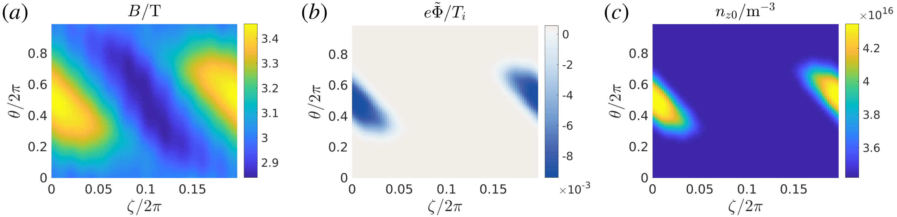
(a) A W7-X standard configuration vacuum field, with (b)
 $\tilde{\unicode[STIX]{x1D6F7}}$
and (c)
 $n_{z0}$
, for
 $\tilde{\unicode[STIX]{x1D6F7}}(B)=\tilde{\unicode[STIX]{x1D6F7}}(B_{0})\text{e}^{-(B-B_{0})^{2}/(2\unicode[STIX]{x1D70E}^{2})}-X$
with
 $B_{0}=B_{\text{max}}$
,
 $\tilde{\unicode[STIX]{x1D6F7}}(B_{0})=-10~\text{V}$
and
 $\unicode[STIX]{x1D70E}=0.1|B_{\text{max}}-B_{\text{min}}|$
,
 $Z=24$
,
 $\langle n_{z}\rangle =3.472\times 10^{16}~\text{m}^{-3}$
and
 $T_{i}=T_{z}=1~\text{keV}$
.
 $X$
is an integration constant set to make
 $\langle \tilde{\unicode[STIX]{x1D6F7}}\rangle =0$
.

We take
 $B$
from a Wendelstein 7-X vacuum field,Footnote
2
and solve the magnetic differential equations for
 $u$
and
 $w$
numerically for this field. The magnetic field in Boozer coordinates (with
 $\unicode[STIX]{x1D701}$
,
 $\unicode[STIX]{x1D703}$
being toroidal and poloidal angle, respectively) is visualized in figure 1, together with an example
 $\tilde{\unicode[STIX]{x1D6F7}}$
and the resulting
 $n_{z0}$
for
 $Z=24$
and
 $\langle n_{z}\rangle =3.472\times 10^{16}~\text{m}^{-3}$
.
To investigate the effects of a localized
 $n_{z}$
distribution, we performed a scan where the amplitude of the potential perturbation is increased. Specifically, the potential perturbation is centred at
 $B_{\text{max}}$
or
 $B_{\text{min}}$
, and the amplitude
 $\tilde{\unicode[STIX]{x1D6F7}}(B_{0})$
is scanned from
 $e\tilde{\unicode[STIX]{x1D6F7}}/T_{z}=-0.1$
to
 $e\tilde{\unicode[STIX]{x1D6F7}}/T_{z}=0.1$
– where a negative/positive sign corresponds to impurities accumulating/decumulating at
 $B_{\text{max}}$
or
 $B_{\text{min}}$
. The ion temperature and density are
 $T_{i}=1~\text{keV}$
and
 $n_{i}=2\times 10^{20}~\text{m}^{-3}$
;
 $m_{i}$
is taken as the proton mass. These values give
 $Z^{2}\langle n_{z}\rangle /n_{i}=0.1$
, so the impurities are trace. For these parameters, the collisionalities are
 $\hat{\unicode[STIX]{x1D708}}_{ii}=0.096$
and
 $\hat{\unicode[STIX]{x1D708}}_{zz}=5.55$
, where we have used
 $L_{\Vert }=(G+\unicode[STIX]{x1D704}I)/B_{00}$
as a proxy for the length scale for parallel variations; here
 $\unicode[STIX]{x1D704}$
is the rotational transform,
 $G$
and
 $I$
are related to the magnetic field and defined in § 2.5 of Helander (Reference Helander2014),
 $B_{00}$
is the
 $n=m=0$
Fourier component of
 $B$
in Boozer coordinates.
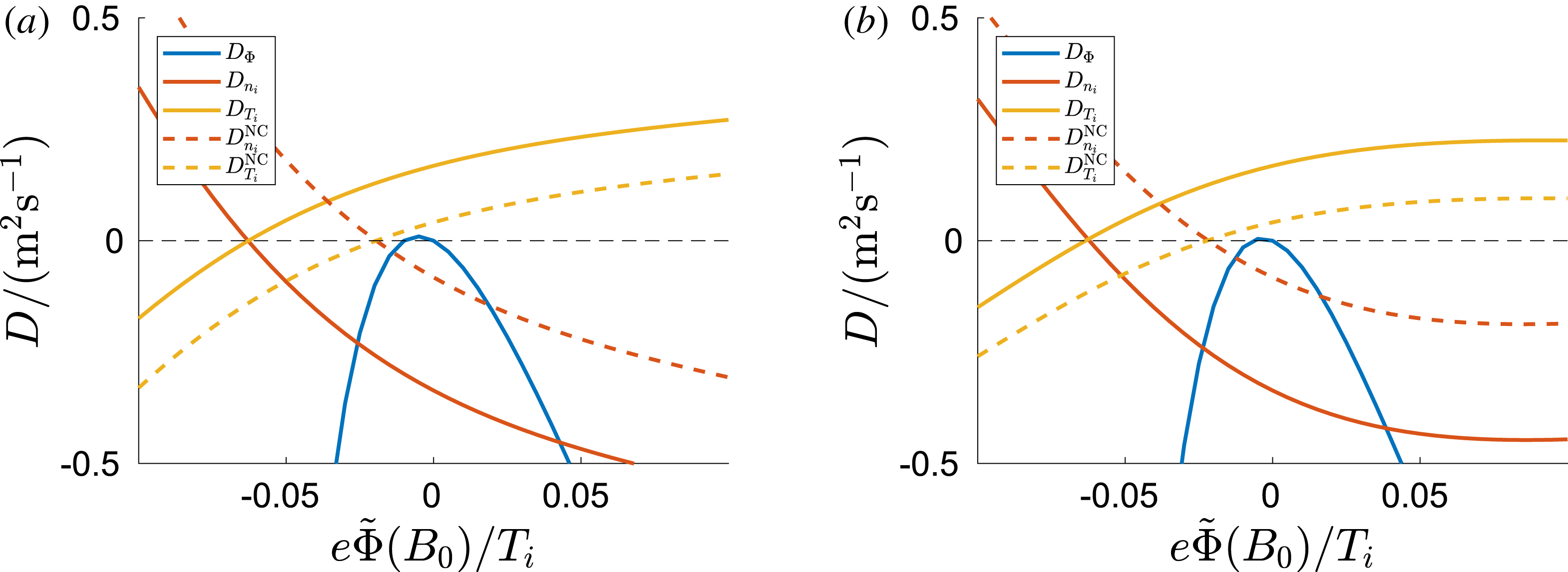
Transport coefficients, for different potential perturbation amplitudes
 $\tilde{\unicode[STIX]{x1D6F7}}(B_{0})$
, for
 $\tilde{\unicode[STIX]{x1D6F7}}$
localized around (a)
 $B_{\text{max}}$
and (b)
 $B_{\text{min}}$
.
 $T_{i}=1~\text{keV}$
and
 $n_{i}=2\times 10^{20}~\text{m}^{-3}$
,
 $\unicode[STIX]{x1D70E}=0.1|B_{\text{max}}-B_{\text{min}}|$
,
 $Z=24$
,
 $\langle n_{z}\rangle =3.472\times 10^{16}~\text{m}^{-3}$
;
 $D^{\text{NC}}$
refers to the neoclassical transport coefficients, while
 $D$
is the sum of classical and neoclassical. At amplitudes roughly within
 $e\tilde{\unicode[STIX]{x1D6F7}}/T_{i}\in [-0.007,0]$
, the flux due to an inward radial electric field is outward but very weak.

The resulting transport coefficients are shown in figure 2. In the figures,
 $D$
(without superscript index) refers to the sum of neoclassical and classical
 $D$
values. For comparison, we also show
 $D^{\text{NC}}$
;
 $D_{N_{z}}$
is not shown, since
 $D_{N_{z}}=-D_{\unicode[STIX]{x1D6F7}}-D_{n_{i}}$
, and the Schwarz inequality causes it to always be non-negative, so that the question of whether impurities accumulate can be answered without its exact value. As indicated in § 5, classical transport is dominant for this field configuration at
 $\tilde{\unicode[STIX]{x1D6F7}}=0$
, but we also see that the transport due to the radial electric field starts to dominate already at
 $e\tilde{\unicode[STIX]{x1D6F7}}(B_{0})/T_{i}\sim 0.02$
. When the radial electric field does not dominate, the impurities will be driven outwards when the temperature gradient is strong enough, i.e. we have temperature screening. Specifically, temperature screening occurs when
 $\text{d}_{\unicode[STIX]{x1D713}}\ln T_{i}\geqslant -D_{n_{i}}\text{d}_{\unicode[STIX]{x1D713}}\ln n_{i}/D_{T_{i}}\approx 2\text{d}_{\unicode[STIX]{x1D713}}\ln n_{i}$
, and thus depends on the ratio
 $D_{n_{i}}/D_{T_{i}}$
. This ratio is equal to
 $-2$
to within
 $1\,\%$
in the
 $\tilde{\unicode[STIX]{x1D6F7}}$
-amplitude window when radial electric field does not dominate, so the temperature screening condition is essentially unaffected, despite the transport coefficients
 $D_{n_{i}}$
and
 $D_{T_{i}}$
varying by approximately
 $25\,\%$
in this window. We also see that both when
 $B_{0}=B_{\text{max}}$
and
 $B_{0}=B_{\text{min}}$
, there is a very narrow amplitude range, approximately
 $e\tilde{\unicode[STIX]{x1D6F7}}(B_{0})/T_{i}\in [-0.007,0]$
, in which the impurity flux due to an inward radial electric field is weakly positive.
From figure 2, we also see that most of the variation in
 $D_{n_{i}}$
and
 $D_{T_{i}}$
comes from the neoclassical flux. This can partly be understood from the simpler form of the classical flux (5.6), where the dependence on
 $n_{z}$
is linear, so that the localized
 $n_{z}$
perturbation due to
 $\tilde{\unicode[STIX]{x1D6F7}}$
merely acts as a weight in the geometric factor
 $\langle n_{z}|\unicode[STIX]{x1D735}\unicode[STIX]{x1D713}|^{2}/B^{2}\rangle$
, which here gives a small effect when integrated over the flux surface. In contrast, the neoclassical flux (4.5) is nonlinear in
 $n_{z}$
, and the total flux through the flux surface is set by a balance between inward and outward fluxes at different points on the flux surface.
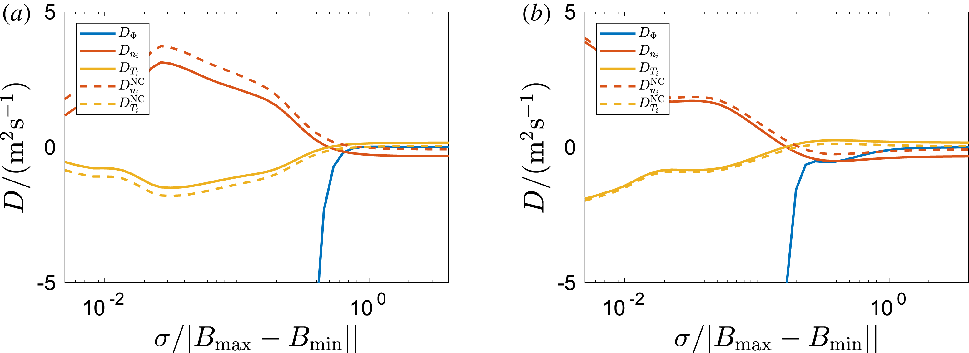
Transport coefficient for varying
 $\unicode[STIX]{x1D70E}$
, for
 $\tilde{\unicode[STIX]{x1D6F7}}$
given by (6.1), with
 $eX/T_{i}=-0.025$
and
 $\tilde{\unicode[STIX]{x1D6F7}}(B_{0})$
set to make
 $\langle \tilde{\unicode[STIX]{x1D6F7}}\rangle =0$
. The potential is centred around (a)
 $B_{\text{max}}$
, and (b)
 $B_{\text{min}}$
. Unless otherwise stated, quantities have the same value as in figure 2.

To investigate the effects of more localized
 $n_{z0}$
, we scanned the width of
 $\tilde{\unicode[STIX]{x1D6F7}}$
, while keeping
 $X$
and
 $\langle n_{z0}\rangle$
constant. For small
 $\unicode[STIX]{x1D70E}$
, this results in
 $n_{z0}$
that are very localized around the extremum of
 $B$
. The result is shown in figure 3. From the figure, we see that
 $D_{\unicode[STIX]{x1D6F7}}^{\text{NC}}$
diverges for localized
 $n_{z0}$
. This is due to the
 $w_{0}^{2}$
terms in
 $D_{\unicode[STIX]{x1D6F7}}^{\text{NC}}$
:
 $n_{z0}w_{0}$
obtained from (2.9) is not localized to regions where
 $n_{z0}$
is localized, which results in a large
 $w_{0}$
where
 $n_{z0}$
is small. In contrast, the
 $D_{n_{i}}^{\text{NC}}$
and
 $D_{T_{i}}^{\text{NC}}$
remains finite, as
 $w_{0}$
only appears together with an
 $n_{z0}$
in those terms. In comparison to the neoclassical transport coefficients, the classical coefficients are only moderately affected by a more localized
 $n_{z0}$
, for the same reasons as discussed in relation to the amplitude scan above.
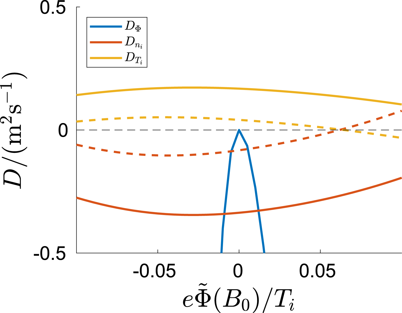
Figure corresponding to figure 2, but with
 $n_{z0}$
concentrated around (or repelled from) the
 $B=(B_{\text{min}}/2+B_{\text{max}}/2)$
contour.

To see whether this conclusion holds for more general
 $n_{z0}$
, we let
 $B_{0}$
in (6.1) be a non-extremum point (within the flux surface), i.e.
 $B_{0}\in (B_{\text{min}},B_{\text{max}})$
. The resulting density distributions
 $n_{z0}$
will be concentrated or repelled from a contours of
 $B$
, rather than points, and do not necessarily represent realistic density variations: rather, they provide simple test cases very different from those considered above, and thus give an indication of how general the above conclusions are.
For
 $B_{0}=B_{\text{min}}/2+B_{\text{max}}/2$
, the resulting
 $D$
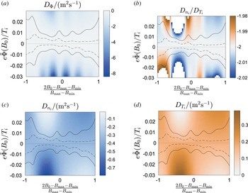
values are displayed in figure 4. Here, the
 $D_{\unicode[STIX]{x1D6F7}}$
increases rapidly with the amplitude, and dominates the flux except for a small interval about
 $0$
. Meanwhile,
 $D_{T_{i}}$
and
 $D_{n_{i}}$
are barely affected, with a slight reduction in magnitude when the impurities are repelled from
 $B_{0}$
.
Transport coefficient when
 $B_{0}$
is changed from
 $B_{\text{min}}$
to
 $B_{\text{max}}$
. Apart from
 $B_{0}$
, quantities have the same values as in figure 2. The black lines indicate potential amplitudes at which the radial electric field starts to dominate: the solid line is where
 $D_{\unicode[STIX]{x1D6F7}}=D_{n_{i}}+D_{T_{i}}$
, the dashed is where
 $10D_{\unicode[STIX]{x1D6F7}}=D_{n_{i}}+D_{T_{i}}$
. (b)
 $D_{n_{i}}/D_{T_{i}}$
, which is within
 $1\,\%$
of
 $2$
for amplitudes where
 $D_{n_{i}}+D_{T_{i}}\geqslant D_{\unicode[STIX]{x1D6F7}}$
(deviations larger than
 $1\,\%$
are white in the figure).

To connect this result to when
 $B_{0}$
is an extremum, we scanned
 $B_{0}$
from
 $B_{\text{min}}$
to
 $B_{\text{max}}$
. The resulting
 $D$
values are shown in figure 5. Looking at
 $D_{\unicode[STIX]{x1D6F7}}$
, we see that as we go from
 $B_{0}=B_{\text{min}}/2+B_{\text{max}}/2$
(
 $x=0$
in the figure) towards the extrema (
 $x=1$
and
 $x=-1$
),
 $D_{\unicode[STIX]{x1D6F7}}$
tends to become less sensitive to the amplitude.
From figure 5(b), we see that for all
 $B_{0}$
,
 $D_{n_{i}}/D_{T_{i}}$
changes by less than
 $1\,\%$
within the amplitude interval where
 $D_{\unicode[STIX]{x1D6F7}}$
is small enough to not notably affect temperature screening (this interval is within or slightly outside the dashed lines, which show where
 $10D_{\unicode[STIX]{x1D6F7}}=D_{n_{i}}+D_{T_{i}}$
).
To conclude, it thus appears that strong
 $\tilde{\unicode[STIX]{x1D6F7}}$
perturbations are likely to lead to strong impurity accumulation if the radial electric field is pointing inwards, and that the condition for temperature screening is essentially unchanged from the
 $\tilde{\unicode[STIX]{x1D6F7}}=0$
case when the
 $\tilde{\unicode[STIX]{x1D6F7}}$
perturbations are weak enough so that the radial electric field is not dominant.
7 Summary and conclusions
We have derived expressions for the radial flux of high-
 $Z$
collisional impurities when the bulk ions are in the
 $1/\unicode[STIX]{x1D708}$
regime. In this limit, the impurity temperature is equilibrated with the bulk ions, while the impurity density can vary within the flux surface. We have derived an expression for the parallel friction force acting on the impurities, which can be used to solve for the impurity density variations on the flux surface, given a mechanism for relating the impurity density to the electrostatic potential.
We considered in detail the trace impurity limit, with the impurity density set by a Boltzmann response to an externally imposed the electrostatic potential. Using simple models for
 $\tilde{\unicode[STIX]{x1D6F7}}$
and a W7-X vacuum field, we have seen that large
 $\tilde{\unicode[STIX]{x1D6F7}}$
amplitudes can cause the radial electric field to substantially contribute to the impurity transport, and lead to impurity accumulation when the radial electric field points inward. For smaller
 $\tilde{\unicode[STIX]{x1D6F7}}$
amplitudes, temperature screening can be effective, and the condition for temperature screening is essentially the same as in the
 $\tilde{\unicode[STIX]{x1D6F7}}=0$
case, meaning that the temperature profile should be at least twice as steep as the density profile for screening to happen. In all cases, the contribution from classical transport is substantial, and even moderate
 $\tilde{\unicode[STIX]{x1D6F7}}$
can cause the electric field to dominate if classical transport is not accounted for.
It is however not straightforward to extrapolate from these results to general
 $\tilde{\unicode[STIX]{x1D6F7}}$
, as the neoclassical impurity flux does not depend linearly on
 $n_{z}$
, so the flux from a general
 $n_{z}$
flux-surface distribution is not a superposition of fluxes from simpler
 $n_{z}$
distributions. Realistic
 $\tilde{\unicode[STIX]{x1D6F7}}$
or
 $n_{z}$
distributions may be needed to evaluate the fluxes accurately, especially when neoclassical transport is comparable to or stronger than the classical. We refer the interested reader to Calvo et al. (Reference Calvo, Parra, Velasco, Alonso and García-Regaña2018), where an LHD equilibrium with a
 $\tilde{\unicode[STIX]{x1D6F7}}$
set-up by particle trapping effects of the bulk ions is considered.
Acknowledgements
The authors are grateful for the fruitful discussions with the authors of Calvo et al. (Reference Calvo, Parra, Velasco, Alonso and García-Regaña2018), who considered the same problem independently of and in parallel to us, from which we have benefited. This work has been carried out within the framework of the EUROfusion Consortium and has received funding from the Euratom research and training programme 2014-2018 under grant agreement no. 633053. The views and opinions expressed herein do not necessarily reflect those of the European Commission. S.B. and I.P. were supported by the International Career Grant of Vetenskapsrådet (Dnr. 330-2014-6313) and I.P. by Marie Sklodowska Curie Actions, Cofund, Project INCA 600398. S.B.’s visit to Greifswald was supported by Chalmersska forskningsfonden.
Appendix A. Solving the ion drift-kinetic equation
In this section, we solve the ion kinetic equation (3.7)–(3.9) for
 $F_{i1(-1)}$
and
 $F_{i1(0)}$
. The solution follows Newton et al. (Reference Newton, Helander, Mollén and Smith2017), but here
 $n_{z}$
is allowed to vary on the flux surface. Since we assume
 $e\tilde{\unicode[STIX]{x1D6F7}}/T_{i}\sim Z^{-1}$
, the potential energy of the bulk ions is approximately constant on the flux surface, and we change variables from
 ${\mathcal{E}}$
,
 $\unicode[STIX]{x1D707}$
to the approximate invariants
 $v$
and
 $\unicode[STIX]{x1D706}$
.
We note that since we only use
 $F_{i1}$
to calculate the ion-impurity friction force, we only need the part of
 $F_{i1}$
that is odd in
 $v_{\Vert }$
. We thus split (3.7)–(3.9) into odd and even equations.
Denoting the odd (even) part of the distribution function with a minus (plus) superscript, the order
 $\hat{\unicode[STIX]{x1D708}}^{-1}$
equations become
 $$\begin{eqnarray}\displaystyle & \displaystyle v_{\Vert }\unicode[STIX]{x1D735}_{\Vert }F_{i1(-1)}^{+}=0 & \displaystyle\end{eqnarray}$$
 $$\begin{eqnarray}\displaystyle & \displaystyle v_{\Vert }\unicode[STIX]{x1D735}_{\Vert }F_{i1(-1)}^{-}=0, & \displaystyle\end{eqnarray}$$
which simply states that
 $F_{i1(-1)}$
is constant along field lines,
 $$\begin{eqnarray}F_{i1(-1)}=F_{i1(-1)}(l_{0}),\end{eqnarray}$$
where
 $l_{0}$
is an arbitrary point on the field line. In the trapped region, this implies that
 $F_{i1(-1)}^{-}=0$
, since it must vanish at bounce points. In the passing region,
 $F_{i1(-1)}(l_{0})$
is set by solvability conditions to the next-order equations.
To order
 $\hat{\unicode[STIX]{x1D708}}^{0}$
, we have that
 $$\begin{eqnarray}\displaystyle & \displaystyle v_{\Vert }\unicode[STIX]{x1D735}_{\Vert }F_{i1(0)}^{+}=C_{i}^{-}[F_{i1(-1)}]. & \displaystyle\end{eqnarray}$$
 $$\begin{eqnarray}\displaystyle & \displaystyle v_{\Vert }\unicode[STIX]{x1D735}_{\Vert }F_{i1(0)}^{-}+\boldsymbol{v}_{d}\boldsymbol{\cdot }\unicode[STIX]{x1D735}f_{i0}=C_{i}^{+}[F_{i1(-1)}]. & \displaystyle\end{eqnarray}$$
In the passing region, the odd and even part of
 $F_{i1(-1)}(l_{0})$
can be determined by acting with
 $\langle B/v_{\Vert }\cdots \rangle$
on equations (A 4)–(A 5), resulting in
 $$\begin{eqnarray}\displaystyle & \displaystyle \left\langle \frac{B}{v_{\Vert }}C_{i}^{-}[F_{i1(-1)}]\right\rangle =0 & \displaystyle\end{eqnarray}$$
 $$\begin{eqnarray}\displaystyle & \displaystyle \left\langle \frac{B}{v_{\Vert }}C_{i}^{+}[F_{i1(-1)}]\right\rangle =\left\langle \frac{B}{v_{\Vert }}\boldsymbol{v}_{d}\boldsymbol{\cdot }\unicode[STIX]{x1D735}\unicode[STIX]{x1D713}\right\rangle \unicode[STIX]{x2202}_{\unicode[STIX]{x1D713}}f_{i0}=0, & \displaystyle\end{eqnarray}$$
where the latter equality follows from writing
 $\boldsymbol{v}_{d}\boldsymbol{\cdot }\unicode[STIX]{x1D735}\unicode[STIX]{x1D713}=v_{\Vert }(\boldsymbol{b}\times \unicode[STIX]{x1D735}\unicode[STIX]{x1D713})\boldsymbol{\cdot }\unicode[STIX]{x1D735}(v_{\Vert }/\unicode[STIX]{x1D6FA}_{i})$
. The odd and even parts of the collision operator are
 $$\begin{eqnarray}\displaystyle & \displaystyle C_{i}^{+}[X]=(\unicode[STIX]{x1D708}_{ii}^{D}+\unicode[STIX]{x1D708}_{iz}^{D}){\mathcal{L}}X^{+} & \displaystyle\end{eqnarray}$$
 $$\begin{eqnarray}\displaystyle & \displaystyle C_{i}^{-}[X]=(\unicode[STIX]{x1D708}_{ii}^{D}+\unicode[STIX]{x1D708}_{iz}^{D}){\mathcal{L}}X^{-}+\frac{m_{i}\,f_{i0}}{T_{i}}v_{\Vert }(\unicode[STIX]{x1D708}_{ii}^{D}U_{\Vert }+\unicode[STIX]{x1D708}_{iz}^{D}V_{z\Vert }), & \displaystyle\end{eqnarray}$$
with
 ${\mathcal{L}}=(2v_{\Vert }/v^{2}B)(\unicode[STIX]{x2202}/\unicode[STIX]{x2202}\unicode[STIX]{x1D706})\unicode[STIX]{x1D706}v_{\Vert }(\unicode[STIX]{x2202}/\unicode[STIX]{x2202}\unicode[STIX]{x1D706})$
. Equation (A 6) implies that
 $F_{i1(-1)}^{+}$
is constant in
 $\unicode[STIX]{x1D706}$
, so that
 $C_{i}^{+}[F_{i1(-1)}]=0$
in the passing region. The same argument applies to
 $F_{i1(-1)}^{-}$
, unless there is a parallel impurity flow in (A 9) to order
 $\hat{\unicode[STIX]{x1D708}}^{-1}$
to act as a source in (A 6). Such order
 $\hat{\unicode[STIX]{x1D708}}^{-1}$
flows cannot arise in the mixed-collisionality regime, so
 $F_{i1(-1)}^{-}=0$
(Newton et al.
Reference Newton, Helander, Mollén and Smith2017). However, to make the
 $F_{i1}$
formulas in this section apply for any impurity collisionality, we will nevertheless allow for
 $F_{i1(-1)}^{-}\neq 0$
below, as it turns out to not be inconvenient to calculate
 $F_{i1(-1)}^{-}$
together with
 $F_{i1(0)}^{-}$
.
To solve for
 $F_{i1(0)}^{-}$
, we note that (A 5) can be formally solved by integrating along a field line; using
 $l$
to denote the distance along the field line, we have
 $$\begin{eqnarray}F_{i1(0)}^{-}(l)=F_{i1(0)}^{-}(l_{0})+\int _{l_{0}}^{l}\frac{\text{d}l^{\prime }}{v_{\Vert }}[C^{+}[F_{1(-1)}]-\boldsymbol{v}_{d}\boldsymbol{\cdot }\unicode[STIX]{x1D735}f_{i0}(l^{\prime })],\end{eqnarray}$$
where the integration constant
 $F_{i1(0)}^{-}(l_{0})$
again is set by the solvability condition of the next-order equation. Taking
 $l_{0}$
to be a bounce point,
 $B(l_{0})=1/\unicode[STIX]{x1D706}$
, we have that
 $F_{i1(0)}^{-}(l_{0})=0$
in the trapped region. To determine
 $F_{i1(0)}^{-}(l_{0})$
the passing region, we again act with
 $\langle B/v_{\Vert }\cdots \rangle$
on the next-order odd equation, which gives
 $$\begin{eqnarray}\left\langle \frac{B}{v_{\Vert }}C_{i}^{-}[F_{i1(0)}]\right\rangle =0.\end{eqnarray}$$
Note that this is essentially the same equation as (A 6). Thus, the total distribution
 $F_{i1}\approx F_{i1(0)}+F_{i1(-1)}$
can be written in the same form as
 $F_{i1(0)}$
, but with an order
 $\hat{\unicode[STIX]{x1D708}}^{-1}$
contribution to the integration constant
 $F_{i1}^{-}(l_{0})\approx F_{i1(-1)}^{-}(l_{0})+F_{i1(0)}^{-}(l_{0})$
. As such, it is in some sense irrelevant whether parts of
 $V_{z\Vert }$
are order
 $\hat{\unicode[STIX]{x1D708}}^{-1}$
or
 $\hat{\unicode[STIX]{x1D708}}^{0}$
, as
 $F_{i1(0)}+F_{i1(-1)}$
is not affected by the way this decomposition of
 $V_{z\Vert }$
is done.
Inserting (A 9) into (A 11) gives the following equation for the integration constant
 $F_{i1}^{-}(l_{0})=F_{i1(-1)}^{-}(l_{0})+F_{i1(0)}^{-}(l_{0})$
 $$\begin{eqnarray}\displaystyle \frac{\unicode[STIX]{x2202}}{\unicode[STIX]{x2202}\unicode[STIX]{x1D706}}F_{i1}^{-}(l_{0}) & = & \displaystyle -\frac{mv^{2}}{\displaystyle 2\left\langle \left[1+\frac{\unicode[STIX]{x1D708}_{iz}^{D}(l)}{\unicode[STIX]{x1D708}_{ii}^{D}}\right]v_{\Vert }\right\rangle }\nonumber\\ \displaystyle & & \displaystyle \times \,\left(\frac{1}{e}\left\langle \left[1+\frac{\unicode[STIX]{x1D708}_{iz}^{D}(l)}{\unicode[STIX]{x1D708}_{ii}^{D}}\right]g_{4}(l,\unicode[STIX]{x1D706})\right\rangle \frac{\unicode[STIX]{x2202}f_{i0}}{\unicode[STIX]{x2202}\unicode[STIX]{x1D713}}+\frac{1}{T_{i}}f_{i0}\left\langle B\left[U_{\Vert }+\frac{\unicode[STIX]{x1D708}_{iz}^{D}(l)}{\unicode[STIX]{x1D708}_{ii}^{D}}V_{z\Vert }\right]\right\rangle \right),\nonumber\\ \displaystyle & & \displaystyle\end{eqnarray}$$
in the passing region. To account for the
 $\boldsymbol{v}_{d}\boldsymbol{\cdot }\unicode[STIX]{x1D735}f_{i0}$
term, we have introduced the geometric function (Nakajima et al.
Reference Nakajima, Okamoto, Todoroki, Nakamura and Wakatani1989)
 $$\begin{eqnarray}g_{4}(\unicode[STIX]{x1D706},l)=v_{\Vert }\int _{l_{0}}^{l}\text{d}l^{\prime }(\boldsymbol{b}\times \unicode[STIX]{x1D735}\unicode[STIX]{x1D713})\boldsymbol{\cdot }\unicode[STIX]{x1D735}\left(\frac{1}{v_{\Vert }}\right).\end{eqnarray}$$
Note that
 $C_{i}^{+}[F_{i1(-1)}]=0$
in this region. In the trapped region, on the other hand,
 $F_{i1}^{-}(l_{0})=0$
but
 $C_{i}^{+}[F_{i1(-1)}]\neq 0$
. However, the
 $C_{i}^{+}[F_{i1(-1)}]$
-term nevertheless gives no contribution to the parallel flow or friction force in this region (Helander, Parra & Newton Reference Helander, Parra and Newton2017b
).
Appendix B. Parallel friction force
Once
 $U_{\Vert }$
and
 $V_{z\Vert }$
are known, we can use (A 10) and (A 12) to directly evaluate the parallel friction force acting on the impurities. From our mass-ratio expanded ion-impurity collision operator (3.2) and the self-adjointness of the Lorentz operator, we have
 $$\begin{eqnarray}\displaystyle R_{iz\Vert } & = & \displaystyle \int \text{d}^{3}vm_{i}v_{\Vert }\unicode[STIX]{x1D708}_{iz}^{D}(v)\left(\frac{m_{i}v_{\Vert }V_{z\Vert }}{T_{i}}f_{i0}-F_{i1}^{-}\right)\nonumber\\ \displaystyle & = & \displaystyle \frac{n_{i}m_{i}}{\unicode[STIX]{x1D70F}_{iz}}\left(V_{z\Vert }-\frac{T_{i}}{e}\left[A_{i1}-\frac{3}{2}A_{i2}\right]Bu-BP(\unicode[STIX]{x1D713})\right),\end{eqnarray}$$
where
 $u$
satisfies the magnetic equation (3.11) and
 $P$
is a flux function which contains the contribution from the integration constant
 $F_{i1}^{-}(l_{0})$
 $$\begin{eqnarray}P(\unicode[STIX]{x1D713})\equiv \frac{\unicode[STIX]{x1D70F}_{iz}}{Bn_{i}}\int \text{d}^{3}vv_{\Vert }\unicode[STIX]{x1D708}_{iz}^{D}(v)F_{i1}^{-}(l_{0}).\end{eqnarray}$$
 $P(\unicode[STIX]{x1D713})$
can be evaluated using (A 12) and partial integration in
 $\unicode[STIX]{x1D706}$
 $$\begin{eqnarray}P(\unicode[STIX]{x1D713})=\frac{\langle BU_{\Vert }\rangle }{\langle B^{2}\rangle }b_{1}+\frac{\langle \unicode[STIX]{x1D6FC}BV_{z\Vert }\rangle }{\langle B^{2}\rangle }b_{4}+\frac{T_{i}}{e}\frac{A_{1i}-\frac{5}{2}A_{2i}}{\langle B^{2}\rangle }b_{2}+\frac{T_{i}}{e}\frac{A_{2i}}{\langle B^{2}\rangle }b_{3},\end{eqnarray}$$
where we have introduced
 $$\begin{eqnarray}\displaystyle & \displaystyle b_{1}=\frac{m\unicode[STIX]{x03C0}\langle B^{2}\rangle }{n_{i}T_{i}\{\unicode[STIX]{x1D708}_{D}^{iz}\}}\int _{0}^{\infty }\text{d}vv^{4}\unicode[STIX]{x1D708}_{D}^{iz}\,f_{i0}\int _{0}^{1/B_{\text{max}}}\text{d}\unicode[STIX]{x1D706}\unicode[STIX]{x1D706}\frac{1}{\displaystyle \langle \unicode[STIX]{x1D709}\rangle +\left\langle \frac{\unicode[STIX]{x1D708}_{iz}^{D}}{\unicode[STIX]{x1D708}_{ii}^{D}}\unicode[STIX]{x1D709}\right\rangle } & \displaystyle\end{eqnarray}$$
 $$\begin{eqnarray}\displaystyle & \displaystyle b_{2}=\frac{m\unicode[STIX]{x03C0}\langle B^{2}\rangle }{n_{i}T_{i}\{\unicode[STIX]{x1D708}_{D}^{iz}\}}\int _{0}^{\infty }\text{d}vv^{4}\unicode[STIX]{x1D708}_{D}^{iz}\,f_{i0}\int _{0}^{1/B_{\text{max}}}\text{d}\unicode[STIX]{x1D706}\unicode[STIX]{x1D706}\frac{\displaystyle \left[\langle g_{4}\rangle +\left\langle \frac{\unicode[STIX]{x1D708}_{iz}^{D}}{\unicode[STIX]{x1D708}_{ii}^{D}}g_{4}\right\rangle \right]}{\displaystyle \langle \unicode[STIX]{x1D709}\rangle +\left\langle \frac{\unicode[STIX]{x1D708}_{iz}^{D}}{\unicode[STIX]{x1D708}_{ii}^{D}}\unicode[STIX]{x1D709}\right\rangle } & \displaystyle\end{eqnarray}$$
 $$\begin{eqnarray}\displaystyle & \displaystyle b_{3}=\frac{m\unicode[STIX]{x03C0}\langle B^{2}\rangle }{n_{i}T_{i}\{\unicode[STIX]{x1D708}_{D}^{iz}\}}\int _{0}^{\infty }\text{d}vv^{4}\frac{m_{i}v^{2}}{2T_{i}}\unicode[STIX]{x1D708}_{D}^{iz}\,f_{i0}\int _{0}^{1/B_{\text{max}}}\text{d}\unicode[STIX]{x1D706}\unicode[STIX]{x1D706}\frac{\displaystyle \left[\langle g_{4}\rangle +\left\langle \frac{\unicode[STIX]{x1D708}_{iz}^{D}}{\unicode[STIX]{x1D708}_{ii}^{D}}g_{4}\right\rangle \right]}{\displaystyle \langle \unicode[STIX]{x1D709}\rangle +\left\langle \frac{\unicode[STIX]{x1D708}_{iz}^{D}}{\unicode[STIX]{x1D708}_{ii}^{D}}\unicode[STIX]{x1D709}\right\rangle } & \displaystyle\end{eqnarray}$$
 $$\begin{eqnarray}\displaystyle & \displaystyle b_{4}=\frac{m\unicode[STIX]{x03C0}\langle B^{2}\rangle }{Z^{2}n_{z}T_{i}\{\unicode[STIX]{x1D708}_{D}^{iz}\}}\int _{0}^{\infty }\text{d}vv^{4}\unicode[STIX]{x1D708}_{D}^{iz}\frac{\unicode[STIX]{x1D708}_{D}^{iz}}{\unicode[STIX]{x1D708}_{ii}^{D}}\,f_{i0}\int _{0}^{1/B_{\text{max}}}\text{d}\unicode[STIX]{x1D706}\unicode[STIX]{x1D706}\frac{1}{\displaystyle \langle \unicode[STIX]{x1D709}\rangle +\left\langle \frac{\unicode[STIX]{x1D708}_{iz}^{D}}{\unicode[STIX]{x1D708}_{ii}^{D}}\unicode[STIX]{x1D709}\right\rangle }, & \displaystyle\end{eqnarray}$$
with
 $\unicode[STIX]{x1D709}=\boldsymbol{v}\boldsymbol{\cdot }\boldsymbol{b}/v$
. The velocity average
 $\{\cdot \}$
is defined as
 $$\begin{eqnarray}\{F(v)\}\equiv \frac{8}{3\sqrt{\unicode[STIX]{x03C0}}}\int _{0}^{\infty }\text{d}xF(x)x^{4}\text{e}^{-x^{2}},\end{eqnarray}$$
where
 $x=v/v_{Ti}$
.
To have the boundary terms from the partial integration disappear in (B 3), we have defined
 $l_{0}$
through
 $B(l_{0})=B_{\text{max}}$
. This makes our choice of
 $l_{0}$
continuous when going from the trapped to the passing region, and thus ensures that
 $F_{i1}^{-}(l_{0})$
is zero at the trapped–passing boundary
 $\unicode[STIX]{x1D706}=1/B_{\text{max}}$
.
Appendix C. Momentum restoring term
$U_{\Vert }$

The momentum restoring term in the ion–ion model collision operator (3.5) is calculated so that ion–ion collisions conserve momentum. Specifically, we have
 $$\begin{eqnarray}U_{\Vert }=\frac{1}{n_{i}\{\unicode[STIX]{x1D708}_{D}^{ii}\}}\int \text{d}^{3}vv_{\Vert }\unicode[STIX]{x1D708}_{D}^{ii}F_{i1}^{-}.\end{eqnarray}$$
Inserting
 $F_{i1}^{-}$
from (A 10) and using (A 12), we get
 $$\begin{eqnarray}\displaystyle & & \displaystyle \langle BU_{\Vert }\rangle (1-a_{1})\nonumber\\ \displaystyle & & \displaystyle \quad =\frac{T_{i}}{e}\left([a_{2}+\langle uB^{2}\rangle ]A_{1i}+\left[a_{3}-\frac{5}{2}a_{2}-\langle uB^{2}\rangle \unicode[STIX]{x1D702}\right]A_{2i}\right)+a_{4}\langle \unicode[STIX]{x1D6FC}BV_{z\Vert }\rangle ,\end{eqnarray}$$
where we have defined the geometry–impurity-dependent flux-surface constants
 $$\begin{eqnarray}\displaystyle & \displaystyle a_{1}=\frac{m\unicode[STIX]{x03C0}\langle B^{2}\rangle }{n_{i}T_{i}\{\unicode[STIX]{x1D708}_{D}^{ii}\}}\int _{0}^{\infty }\text{d}vv^{4}\unicode[STIX]{x1D708}_{D}^{ii}\,f_{i0}\int _{0}^{1/B_{\text{max}}}\text{d}\unicode[STIX]{x1D706}\unicode[STIX]{x1D706}\frac{1}{\displaystyle \langle \unicode[STIX]{x1D709}\rangle +\left\langle \frac{\unicode[STIX]{x1D708}_{iz}^{D}}{\unicode[STIX]{x1D708}_{ii}^{D}}\unicode[STIX]{x1D709}\right\rangle } & \displaystyle\end{eqnarray}$$
 $$\begin{eqnarray}\displaystyle & \displaystyle a_{2}=\frac{m\unicode[STIX]{x03C0}\langle B^{2}\rangle }{n_{i}T_{i}\{\unicode[STIX]{x1D708}_{D}^{ii}\}}\int _{0}^{\infty }\text{d}vv^{4}\unicode[STIX]{x1D708}_{D}^{ii}\,f_{i0}\int _{0}^{1/B_{\text{max}}}\text{d}\unicode[STIX]{x1D706}\unicode[STIX]{x1D706}\frac{\displaystyle \left[\langle g_{4}\rangle +\left\langle \frac{\unicode[STIX]{x1D708}_{iz}^{D}}{\unicode[STIX]{x1D708}_{ii}^{D}}g_{4}\right\rangle \right]}{\displaystyle \langle \unicode[STIX]{x1D709}\rangle +\left\langle \frac{\unicode[STIX]{x1D708}_{iz}^{D}}{\unicode[STIX]{x1D708}_{ii}^{D}}\unicode[STIX]{x1D709}\right\rangle } & \displaystyle\end{eqnarray}$$
 $$\begin{eqnarray}\displaystyle & \displaystyle a_{3}=\frac{m\unicode[STIX]{x03C0}\langle B^{2}\rangle }{n_{i}T_{i}\{\unicode[STIX]{x1D708}_{D}^{ii}\}}\int _{0}^{\infty }\text{d}vv^{4}\frac{m_{i}v^{2}}{2T_{i}}\unicode[STIX]{x1D708}_{D}^{ii}\,f_{i0}\int _{0}^{1/B_{\text{max}}}\text{d}\unicode[STIX]{x1D706}\unicode[STIX]{x1D706}\frac{\displaystyle \left[\langle g_{4}\rangle +\left\langle \frac{\unicode[STIX]{x1D708}_{iz}^{D}}{\unicode[STIX]{x1D708}_{ii}^{D}}g_{4}\right\rangle \right]}{\displaystyle \langle \unicode[STIX]{x1D709}\rangle +\left\langle \frac{\unicode[STIX]{x1D708}_{iz}^{D}}{\unicode[STIX]{x1D708}_{ii}^{D}}\unicode[STIX]{x1D709}\right\rangle } & \displaystyle\end{eqnarray}$$
 $$\begin{eqnarray}\displaystyle & \displaystyle a_{4}=\frac{m\unicode[STIX]{x03C0}\langle B^{2}\rangle }{Z^{2}n_{z}T_{i}\{\unicode[STIX]{x1D708}_{D}^{ii}\}}\int _{0}^{\infty }\text{d}vv^{4}\unicode[STIX]{x1D708}_{iz}^{D}\,f_{i0}\int _{0}^{1/B_{\text{max}}}\text{d}\unicode[STIX]{x1D706}\unicode[STIX]{x1D706}\frac{1}{\displaystyle \langle \unicode[STIX]{x1D709}\rangle +\left\langle \frac{\unicode[STIX]{x1D708}_{iz}^{D}}{\unicode[STIX]{x1D708}_{ii}^{D}}\unicode[STIX]{x1D709}\right\rangle }. & \displaystyle\end{eqnarray}$$
Appendix D. Solvability condition and
$K_{z}$

Equation (2.12) specifies
 $V_{z\Vert }$
up to a flux function
 $K_{z}$
(cf. (2.14)). This
 $K_{z}$
can be determined from solvability condition of (2.2), which states that
 $$\begin{eqnarray}\left\langle \frac{BR_{z\Vert }}{n_{z}}\right\rangle =0.\end{eqnarray}$$
Inserting (3.10), the solvability condition becomes
 $$\begin{eqnarray}\frac{n_{i}m_{i}}{n_{z}\unicode[STIX]{x1D70F}_{iz}}\left(\langle BV_{z\Vert }\rangle -\frac{T_{i}}{e}\left[A_{i1}-\frac{3}{2}A_{i2}\right]\langle uB^{2}\rangle -\langle B^{2}\rangle P(\unicode[STIX]{x1D713})\right)=0.\end{eqnarray}$$
In the
 $\unicode[STIX]{x1D6E5}\ll 1$
limit, we can insert our expression for
 $V_{z\Vert }$
, (2.14), to solve for
 $K_{z}$
. This results in (3.13), where we have defined
 $$\begin{eqnarray}\displaystyle & \displaystyle c_{1}=b_{1}+a_{1}c_{1}\;\Longrightarrow \;c_{1}=b_{1}/(1-a_{1}), & \displaystyle\end{eqnarray}$$
 $$\begin{eqnarray}\displaystyle & \displaystyle c_{2}=b_{2}+a_{2}c_{1}, & \displaystyle\end{eqnarray}$$
 $$\begin{eqnarray}\displaystyle & \displaystyle c_{3}=b_{3}+a_{3}c_{1}, & \displaystyle\end{eqnarray}$$
 $$\begin{eqnarray}\displaystyle & \displaystyle c_{4}=b_{4}+a_{4}c_{1}, & \displaystyle\end{eqnarray}$$
for the sake of compactness.
Appendix E. Trace impurity limit of some expressions
In the trace impurity limit,
 $\unicode[STIX]{x1D6FC}\equiv Z^{2}n_{z}/n_{i}\ll 1$
, the
 $a_{i}$
,
 $b_{j}$
and
 $c_{k}$
terms simplify considerably, yielding an expression for
 $K_{z}$
in terms of standard geometry functions. Specifically,
 $$\begin{eqnarray}\displaystyle & \displaystyle a_{1}=b_{1}=f_{c}, & \displaystyle\end{eqnarray}$$
 $$\begin{eqnarray}\displaystyle & \displaystyle a_{2}=b_{2}=f_{s}, & \displaystyle\end{eqnarray}$$
 $$\begin{eqnarray}\displaystyle & \displaystyle a_{3}=f_{s}({\textstyle \frac{5}{2}}-\unicode[STIX]{x1D702}), & \displaystyle\end{eqnarray}$$
 $$\begin{eqnarray}\displaystyle & \displaystyle b_{3}=f_{s}, & \displaystyle\end{eqnarray}$$
 $$\begin{eqnarray}\displaystyle & \displaystyle a_{4}=\frac{f_{c}}{\unicode[STIX]{x1D6FC}}\frac{\{\unicode[STIX]{x1D708}_{D}^{iz}\}}{\{\unicode[STIX]{x1D708}_{D}^{ii}\}}, & \displaystyle\end{eqnarray}$$
 $$\begin{eqnarray}\displaystyle & \displaystyle b_{4}=\frac{f_{c}}{\unicode[STIX]{x1D6FC}}\frac{\{{\unicode[STIX]{x1D708}_{D}^{iz}}^{2}/\unicode[STIX]{x1D708}_{D}^{ii}\}}{\{\unicode[STIX]{x1D708}_{D}^{iz}\}}. & \displaystyle\end{eqnarray}$$
Note that
 $a_{4}$
and
 $b_{4}$
only appear in terms containing
 $\unicode[STIX]{x1D6FC}$
, which are negligible in the trace limit. Here,
 $$\begin{eqnarray}\displaystyle & \displaystyle f_{c}=\frac{3\langle B^{2}\rangle }{4}\int _{0}^{1/B_{\text{max}}}\text{d}\unicode[STIX]{x1D706}\frac{\unicode[STIX]{x1D706}}{\langle \unicode[STIX]{x1D709}\rangle } & \displaystyle\end{eqnarray}$$
 $$\begin{eqnarray}\displaystyle & \displaystyle f_{s}=\frac{3\langle B^{2}\rangle }{4}\int _{0}^{1/B_{\text{max}}}\text{d}\unicode[STIX]{x1D706}\frac{\unicode[STIX]{x1D706}\langle g_{4}\rangle }{\langle \unicode[STIX]{x1D709}\rangle }, & \displaystyle\end{eqnarray}$$
are standard functions of geometry.
With this, we have that
 $$\begin{eqnarray}\displaystyle & \displaystyle c_{1}=\frac{f_{c}}{1-f_{c}}, & \displaystyle\end{eqnarray}$$
 $$\begin{eqnarray}\displaystyle & \displaystyle c_{2}=\frac{f_{s}}{1-f_{c}}, & \displaystyle\end{eqnarray}$$
 $$\begin{eqnarray}\displaystyle & \displaystyle c_{3}=\frac{f_{s}}{1-f_{c}}\left[1+f_{c}\left(\frac{3}{2}-\unicode[STIX]{x1D702}\right)\right], & \displaystyle\end{eqnarray}$$
 $$\begin{eqnarray}\displaystyle & \displaystyle c_{4}=\frac{f_{c}}{\unicode[STIX]{x1D6FC}}\left(\frac{\{{\unicode[STIX]{x1D708}_{D}^{iz}}^{2}/\unicode[STIX]{x1D708}_{D}^{ii}\}}{\{\unicode[STIX]{x1D708}_{D}^{iz}\}}+\frac{f_{c}}{1-f_{c}}\frac{\{\unicode[STIX]{x1D708}_{D}^{iz}\}}{\{\unicode[STIX]{x1D708}_{D}^{ii}\}}\right), & \displaystyle\end{eqnarray}$$
and
 $K_{z}$
becomes
 $$\begin{eqnarray}\displaystyle & & \displaystyle K_{z}(\unicode[STIX]{x1D713})\left\langle \frac{B^{2}}{n_{z}}\right\rangle \nonumber\\ \displaystyle & & \displaystyle \quad =\frac{T_{i}}{e}[f_{s}+\langle uB^{2}\rangle ]\left(\left[\frac{f_{c}}{1-f_{c}}+1\right]A_{1i}-\left[\frac{\unicode[STIX]{x1D702}f_{c}}{1-f_{c}}+\frac{3}{2}\right]A_{2i}\right)-\frac{\text{d}\langle \unicode[STIX]{x1D6F7}\rangle }{\text{d}\unicode[STIX]{x1D713}}\langle wB^{2}\rangle ,\nonumber\\ \displaystyle & & \displaystyle\end{eqnarray}$$
which results in the friction force
 $$\begin{eqnarray}\displaystyle & & \displaystyle R_{iz,\Vert }\frac{\unicode[STIX]{x1D70F}_{iz}}{n_{i}m_{i}}=\left(w-\frac{\langle wB^{2}\rangle }{\displaystyle n_{z}\left\langle \frac{B^{2}}{n_{z}}\right\rangle }\right)B\frac{\text{d}\langle \unicode[STIX]{x1D6F7}\rangle }{\text{d}\unicode[STIX]{x1D713}}\nonumber\\ \displaystyle & & \displaystyle \qquad +\,\left(\frac{\langle uB^{2}\rangle }{\langle B^{2}\rangle }-u+\left(\frac{1}{\displaystyle n_{z}\left\langle \frac{B^{2}}{n_{z}}\right\rangle }-\frac{1}{\langle B^{2}\rangle }\right)[f_{s}+\langle uB^{2}\rangle ]\left[\frac{f_{c}}{1-f_{c}}+1\right]\right)B\frac{T_{i}}{e}A_{i1}\nonumber\\ \displaystyle & & \displaystyle \qquad -\,\left(\frac{3}{2}\frac{\langle uB^{2}\rangle }{\langle B^{2}\rangle }-\frac{3}{2}u+\left(\frac{1}{\displaystyle n_{z}\left\langle \frac{B^{2}}{n_{z}}\right\rangle }-\frac{1}{\langle B^{2}\rangle }\right)[f_{s}+\langle uB^{2}\rangle ]\left[\frac{\unicode[STIX]{x1D702}f_{c}}{1-f_{c}}+\frac{3}{2}\right]\right)B\frac{T_{i}}{e}A_{i2}.\nonumber\\ \displaystyle & & \displaystyle\end{eqnarray}$$