1. Introduction

The theoretical frameworks of computationalism and connectionism are often construed as a search for cognitive mechanisms, the specific structures and processes from which cognitive phenomena arise. In contrast, the framework of dynamicism is generally understood to be a search for principles or laws—mathematical regularities that govern the way cognitive phenomena unfold over time. In recent philosophical discourse, this difference between traditional and dynamical cognitive science has been framed as a difference in scientific explanation: whereas computationalist and connectionist explanations are mechanistic explanations, dynamical explanations take the form of covering-law explanations (for discussion, see van Gelder Reference van Gelder1995, Reference van Gelder1998; Clark Reference Clark1997, Reference Clark1998; Bechtel Reference Bechtel1998; Bechtel and Abrahamsen Reference Bechtel and Abrahamsen2002; Chemero and Silberstein Reference Chemero and Silberstein2008; Walmsley Reference Walmsley2008; Chemero Reference Chemero2009).

In this article, I challenge the received view of dynamical explanation. After briefly outlining the principles of covering-law explanation and mechanistic explanation in section 2, in section 3 I introduce a well-known dynamical model—the Haken-Kelso-Bunz (HKB) model of coordination dynamics (Haken, Kelso, and Bunz Reference Haken, Kelso and Bunz1985; Kelso Reference Kelso1995)—that is regularly used to articulate and promote the received view. Although this model is often considered to be a paradigmatic example of dynamical explanation, in section 4 I introduce two very different dynamical explanations: Thelen et al.'s (Reference Thelen, Schöner, Scheier and Smith2001) explanation of infant perseverative reaching and Beer's (Reference Beer2003) explanation of perceptual categorization in a minimally cognitive agent. Although both of these dynamical explanations invoke the mathematical tools and concepts of dynamical systems theory, they resemble mechanistic explanations. Therefore, the received view is misleading: although the mathematical tools and concepts of dynamical systems theory are frequently used to describe principles and laws, they are also sometimes used to describe cognitive mechanisms.

Insofar as some dynamical explanations are mechanistic in nature, they have much in common with traditional computational and connectionist explanations. Among others, like other mechanistic explanations in cognitive science, these dynamical explanations are reductive explanations (Craver Reference Craver2007; Bechtel Reference Bechtel2008) and may be amenable to representation hunting (Chemero and Silberstein Reference Chemero and Silberstein2008). Nevertheless, this does not mean that dynamicist research is not interestingly novel and important. Indeed, in section 5 I show that dynamical explanations are well suited for describing extended mechanisms whose components are distributed across brain, body, and the environment. Moreover, I argue that dynamical explanations may be uniquely able to describe mechanisms whose components are engaged in complex relationships of continuous reciprocal causation (Clark Reference Clark1997). Therefore, a closer look at dynamical cognitive science will reveal that the extant philosophical conception of mechanistic explanation may have underestimated practicing scientists’ willingness and ability to describe increasingly complex and distributed cognitive mechanisms.

2. Covering-Law Explanation, Mechanistic Explanation, and Traditional Cognitive Science

According to the principles of covering-law explanation, scientific explanation involves the subsumption of a target phenomenon under natural law. That is, a phenomenon is explained when it can be logically deduced from statements of relevant antecedent conditions and one or more laws of nature (Hempel and Oppenheim Reference Hempel and Oppenheim1948). Two aspects of this conception are worth highlighting. First, saying that a phenomenon is explained when it can be logically deduced is tantamount to saying that a phenomenon can be explained when it can be (or could have been) predicted. Second, although “law of nature” has proven to be a notion of significant philosophical controversy, the core idea is one of a highly general, counterfactual-supporting regularity (for discussion, see Cartwright Reference Cartwright1983; Salmon Reference Salmon1989). Thus construed, Newton's explanation of celestial motion is a paradigmatic example of covering-law explanation: his laws of motion and universal gravitation predict not only the Earth's effect on the motion of the moon but also (purport to) predict the relative effects between any physical objects in actual and counterfactual circumstances.

Alas, it is becoming increasingly clear that the principles of covering-law explanation are of limited use for understanding contemporary cognitive science. Although many aspects of cognitive scientific practice are concerned with the discovery of lawlike behavioral regularities, cognitive scientists tend to treat such regularities—sometimes also called effects—not as explanations but as explanatory targets (Cummins Reference Cummins, Keil and Wilson2000). Indeed, after having been discovered, behavioral regularities are typically explained by describing the mechanisms responsible therefore (Bechtel and Richardson Reference Bechtel and Richardson1993; Machamer, Darden, and Craver Reference Machamer, Darden and Craver2000; Craver Reference Craver2007; Wright and Bechtel Reference Wright, Bechtel and Thagard2007). One particularly influential conception of mechanism is due to William Bechtel: “A mechanism is a structure performing a function in virtue of its component parts, component operations, and their organization. The orchestrated functioning of the mechanism, manifested in patterns of change over time in properties of its parts and operations, is responsible for one or more phenomena” (Bechtel and Abrahamsen Reference Bechtel and Abrahamsen2010, 323; see also Machamer et al. Reference Machamer, Darden and Craver2000; Bechtel and Abrahamsen Reference Bechtel and Abrahamsen2005; Craver Reference Craver2007). In this conception, mechanistic explanation consists of describing the particular organized collection of parts and operations that is responsible for the behavioral regularity being explained.

Mechanistic explanation is by no means trivial. Although scientists may be able to observe that a complex system exhibits a particular behavioral regularity, they may not know which features of that system are involved in producing it. That is, before it can be described, the mechanism responsible for a behavioral regularity has to be discovered. The discovery of mechanisms is frequently facilitated by the explanatory heuristics of decomposition and localization (Bechtel and Richardson Reference Bechtel and Richardson1993), the former of which comes in two forms. Structural decomposition involves breaking a complex system down into a collection of simpler subsystems or parts. But not all structural decompositions lead to the discovery of a mechanism; the parts being revealed should be working parts, meaning they should behave in ways that contribute toward the production of the behavioral phenomenon being explained (Craver Reference Craver2007). Therefore, structural decomposition is usually followed by an attempt to characterize the behavior of individual parts so as to show that they are in fact the working parts of a mechanism. In contrast, functional decomposition involves redescribing the behavioral phenomenon as a series or organized collection of simpler behaviors or operations. Importantly, functional decomposition leads to the discovery of a mechanism only if the operations being posited are actually realized in the system from which the phenomenon arises. One way of showing that this is the case is to localize individual operations in corresponding parts—thus simultaneously showing that the operations are realized in the system and that the parts with which those operations are identified are in fact working parts of a mechanism. Of course, such straightforward localization is not always feasible; scientists frequently have to find more roundabout ways of showing that a given collection of operations is actually realized in the system from which the target phenomenon arises (for discussion, see Bechtel and Richardson Reference Bechtel and Richardson1993; Bechtel and Abrahamsen Reference Bechtel and Abrahamsen2005; Craver Reference Craver2007).

A better understanding of mechanisms and mechanistic explanation can be attained by considering some examples from traditional cognitive science. In classical computationalism, functional decomposition is achieved through the practice of computational modeling, in which the target phenomenon is reproduced by way of an organized series of algorithmic operations on symbolic representations (Cummins Reference Cummins1983). Frequently, computational models are accompanied by a stated commitment, although rarely an explicit attempt, to identify individual operations with specific neurobiological structures—consider David Marr's (Reference Marr1982) attempt to localize the detection of zero-crossings in the so-called simple cells of the visual cortex. Therefore, computational models specify the component operations of a mechanism that are then (in ideal cases) localized in neurobiological component parts.

Whereas computational models are used to describe a mechanism's component operations, artificial neural network models provide abstract descriptions of the neurobiological systems in which cognitive mechanisms are realized.Footnote ¹ After a neural network model is trained to reproduce a particular behavioral phenomenon, a variety of mathematical techniques can be used to reveal the mechanism responsible for that phenomenon. Consider Jeffrey Elman's (Reference Elman1991) simple recurrent network model of language processing. After training the network to predict the word or word category that immediately follows an English sentence fragment, Elman conducts a principal components analysis of the network's hidden-layer activity to describe three operations: (a) identifying number (singular/plural), (b) identifying noun role (subject/object), and (c) identifying verb type (direct object is required/allowed but not required/precluded). Although each one of these operations is distributed across the network's hidden layer and thus cannot be directly localized in any single neural unit, Elman's analysis shows that items a–c are in fact the component operations of a mechanism for word prediction and that they are realized in the system from which it arises.Footnote ²

3. Dynamical Explanation: The Received View

Whereas classical computationalism and connectionism are both typically construed as a search for cognitive mechanisms, dynamicism has traditionally been viewed as a search for principles and laws. Dynamical explanations consist of dynamical models (sets of differential or difference equations that capture a particular cognitive system's behavior) and dynamical analyses (formal analyses that invoke the tools and concepts of dynamical systems theory to describe the modeled system's abstract mathematical properties).Footnote ³ Consider Scott Kelso's (Reference Kelso1995) dynamical explanation of bimanual coordination, a robust behavioral phenomenon in which the rhythmic oscillatory motion of two opposing index fingers spontaneously becomes coordinated in a way that depends on the frequency of oscillation. At low frequencies, opposing index fingers reliably settle into one of two patterns of motion: an in-phase pattern in which both fingers alternate between simultaneously pointing inward and outward, or an anti-phase pattern that resembles the parallel motion of windshield wipers on most cars. At high oscillation frequencies, in contrast, the index fingers settle into the in-phase pattern only.

Kelso's dynamical explanation of bimanual coordination is grounded on the HKB model of coordination dynamics (Haken et al. Reference Haken, Kelso and Bunz1985). This dynamical model consists of a single differential equation that describes in-phase as well as anti-phase motion and that accurately predicts the phase transitions that occur between low and high frequencies:

In this model, changes in the between-fingers phase relation ϕ (where ° corresponds to perfect in-phase motion and ° corresponds to perfect anti-phase motion) are expressed as a function of a and b (where b/a corresponds to the inverse of the index fingers’ oscillation frequency). A dynamical analysis of the HKB model (fig. 1) shows that bimanual coordination can be understood as a dynamical system with two point attractors when (one each corresponding to in-phase and anti-phase motion), one point attractor when (in-phase motion), and an inverse pitchfork bifurcation that annihilates the anti-phase attractor when .

Figure 1

Vector field diagram of the HKB model with ϕ as the state variable and b/a as the control parameter. When , motion is stable when and ° (in-phase) or ° (anti-phase). In contrast, when , motion is stable only when and ° (in-phase). An inverse pitchfork bifurcation at transforms the anti-phase attractor into an unstable equilibrium point. Figure adapted from Kelso (Reference Kelso1995).

The HKB model accurately describes bimanual coordination and supports a variety of testable predictions. Quantitatively, it predicts the pattern of motion that will be exhibited at any given frequency and initial phase relation. In dynamical terms, for any value of b/a and initial ϕ, it is possible to determine the attractor basin that will constrain ϕ's trajectory through state space. Qualitatively, the model predicts a hysteresis effect in which phase transitions occur when the oscillation frequency changes from low values to high but not when the oscillation frequency changes from high values to low. Once again in dynamical terms, if ϕ begins in the attractor basin corresponding to anti-phase motion and b/a decreases, it is forced to settle into the in-phase attractor when the anti-phase attractor is annihilated; if, in contrast, ϕ begins in the attractor basin corresponding to in-phase motion and b/a increases, it remains in that basin indefinitely.

Kelso's dynamical explanation of bimanual coordination is a clear example of covering-law explanation. First, the HKB model is invoked in patterns of deductive inference that conclude with a description of the target phenomenon. Given any particular oscillation frequency and initial phase relation, it can be used to predict the phase relation that will eventually be observed. Second, the HKB model describes a lawlike regularity that is both counterfactual supporting and highly general. On the one hand, this is because the HKB model's predictive power extends to situations in which one or both fingers are forced out of their regular oscillatory motion; although perturbing ϕ away from its stable in-phase or anti-phase motion temporarily results in a phase relation between 0° and 180°, the structure of the attractor landscape predicts that ϕ will inevitably return to one of those two stable attractors and that it will do so within a predictable amount of time. On the other hand, variations of the same model can be used to describe and predict several kinds of coupled oscillatory motion, including animal locomotion (Kelso Reference Kelso1995), speech production (Port Reference Port2003), and behavioral coordination between individuals (Oullier et al. Reference Oullier, de Guzman, Jantzen, Lagarde, Kelso, Peham, Schöllhorn and Verwey2005). In other words, the HKB model is not restricted to any particular system but rather describes a “general principle of pattern formation” that applies “regardless of what elements are involved in producing the patterns or at what level these patterns are studied or observed” (Kelso Reference Kelso1995, 2). Thus, in general, Kelso's dynamical explanation of bimanual coordination is an example of covering-law explanation because it relies on a lawlike regularity to deduce properties of the target phenomenon.Footnote ⁴

But Kelso's dynamical explanation is more than just a well-known example. A brief review of the relevant philosophical literature demonstrates that the features of this particular dynamical explanation are often assumed to be features of dynamical explanation in general. Building on some of the themes in Kelso's (Reference Kelso1995) seminal book, Tim van Gelder first introduced the HKB model to the philosophical community “to illustrate the dynamical approach to cognition” (Reference van Gelder1998, 616) and to draw an analogy between dynamical explanations of cognition and Newton's law-based explanations of celestial motion. Bechtel (Reference Bechtel1998) was the first to explicitly associate Kelso's brand of dynamicism with the principles of covering-law explanation, and Walmsley recently invoked the HKB model to defend the general claim that “the explanatory goal of dynamical cognitive scientists is to provide covering-law explanations” (Reference Walmsley2008, 343). Chemero and Silberstein have recently appealed to Oullier et al.'s (Reference Oullier, de Guzman, Jantzen, Lagarde, Kelso, Peham, Schöllhorn and Verwey2005) adaptation of the HKB model to illustrate the practices of “a growing minority of cognitive scientists” who “have eschewed mechanical explanations and embraced dynamical systems theory” (Chemero and Silberstein Reference Chemero and Silberstein2008, 11), and Chemero has further articulated this view by characterizing the HKB model “as a unifying model and guide to discovery for [dynamical] cognitive science” (Reference Chemero2009, 86). These remarks indicate just how profound the influence of Kelso's dynamical explanation has been: It has served not only as a template for future empirical and modeling work (e.g., van Rooij, Bongers, and Haselager Reference van Rooij, Bongers and Haselager2002) but also as a paradigmatic example on the basis of which general philosophical claims about dynamicism have been articulated and defended. One such claim is the received view of dynamical explanation, the view that dynamical explanation is just a special case of covering-law explanation.

In the next section I will argue that the received view of dynamical explanation is misleading. Kelso's explanation of bimanual coordination is not in fact representative of dynamical explanation in general, and many dynamical explanations actually resemble mechanistic explanations rather than covering-law explanations. In the meantime, however, it is worth noting that the received view renders dynamical explanation susceptible to a well-known philosophical worry. Recall that, according to the principles of covering-law explanation, a phenomenon is explained when it can be predicted from antecedent conditions and one or more lawlike regularities. Frequently, this predictive ability is afforded by lawlike regularities that are phenomenological in kind—regularities that are specified primarily in terms of the target phenomenon's observable properties (Cartwright Reference Cartwright1983; Craver Reference Craver2006). The HKB model is a case in point: ϕ and b/a each refer to observable features of bimanual coordination itself, rather than to the underlying neural, biomechanical, or other physical structures and processes from which that phenomenon arises. Now, a well-known philosophical worry about phenomenological laws is that they merely describe rather than genuinely explain. But although this mere description worry is already well established in the theoretical literature on dynamicism (see, e.g., Eliasmith Reference Eliasmith1996; Dietrich and Markman Reference Dietrich and Markman2001; van Leeuwen Reference van Leeuwen2005), it is frequently brushed aside by proponents of dynamical explanation who appeal to the fact that even phenomenological laws may support counterfactuals (see, e.g., Clark Reference Clark1997; Walmsley Reference Walmsley2008; Chemero Reference Chemero2009). Because phenomenological laws like the one expressed by the HKB model extend to counterfactual circumstances, they go beyond describing what is actually observed and therefore do more than merely describe the target phenomenon.

Unfortunately, this simple appeal to counterfactuals fails to address the core intuition behind the mere description worry. In particular, it is easy to think that covering-law explanations based on phenomenological laws leave something important to be desired: “Because phenomenal models summarize the phenomenon to be explained, they typically allow one to answer some [what-if-things-had-been-different] questions. But an explanation shows why the relations are as they are in the phenomenal model, and so reveals conditions under which those relations might change or fail to hold altogether” (Craver Reference Craver2006, 358). That is, although a phenomenological law may predict what happens in actual and counterfactual circumstances, it often remains unclear why the law applies in the first place. Put differently, phenomenological laws by themselves provide no means of determining when they can or cannot be used in deductive inferences about the target phenomenon. Consider once again Kelso's dynamical explanation of bimanual coordination. The HKB model can be used to deduce properties of the target phenomenon just because moving index fingers can be understood as a system of coupled oscillators. Although this is explicit in Kelso's (Reference Kelso1995) extended discussion of the way in which the HKB model was originally derived, the model itself does not provide any means of determining whether a given system can or cannot be understood as a system of coupled oscillators. In comparison, a (hypothetical) description of the neurobiological and biomechanical mechanisms responsible for bimanual coordination would likely provide a description that resembles a system of coupled oscillators. Unlike covering-law explanations based on phenomenological laws, mechanistic explanations provide a means of determining which systems fall under the scope of the explanation and when they do so. As long as dynamical explanation is viewed as a form of covering-law explanation as the received view suggests, the mere description worry looms.

Of course, the mere description worry can be resisted by stipulating that covering-law explanations (even those that are grounded on phenomenological laws) qualify as genuine explanations. This seems to be the view espoused by philosophical proponents of explanatory pluralism (see, e.g., Chemero and Silberstein Reference Chemero and Silberstein2008), as well as (implicitly or explicitly) by practicing cognitive scientists who choose to employ various descriptive (explanatory?) techniques to accommodate different kinds of phenomena. Short of adopting this kind of pluralist stance, however, the received view of dynamical explanation implies that dynamicist researchers should more thoroughly engage in well-established philosophical worries about covering-law explanation.

4. Dynamical Explanation as Mechanistic Explanation

Before proceeding to cases of dynamical explanation that are mechanistic rather than covering-law in nature, it is important to recognize that there are no a priori reasons to deny that dynamical models and dynamical analyses can be used to provide mechanistic explanations of cognitive phenomena. As Wright and Bechtel (Reference Wright, Bechtel and Thagard2007) go to great lengths to impress, mechanistic explanation is an epistemic activity that centers on the practice of describing a mechanism. Such description can be achieved via a variety of descriptive schemes, including verbal characterizations, schematic box-and-arrow diagrams, more-or-less detailed pictures, and physical or simulated two- and three-dimensional models. The differential (or difference) equations that constitute a dynamical model—as well as the mathematical constructs and graphical representations that figure in dynamical analyses—are, I claim, equally viable descriptive schemes. Variables and parameters can be used to describe structural and functional properties (e.g., size, location, velocity, activation) of the parts and operations of a mechanism, and differential equations can be used to capture spatial and temporal relations between those properties as well as to describe the way they change over time.Footnote ⁵ Likewise, graphical representations such as state-space trajectories, attractor landscapes, bifurcation diagrams, and so on—the representational currency of dynamical analysis—can be used in much the same way. The general point is this: like English, the mathematics of dynamical systems theory is a language, an important feature of which is its capacity to represent. What is being represented—a mechanism, law of nature, or my neighbor's pet iguana—is not determined by the language being used but by the way in which tokens of that language are interpreted. The claim at the heart of my argument is that the differential equations and graphical representations that figure in many dynamical explanations can be, in principle as well as in practice, interpreted as representations of cognitive mechanisms.

One more preliminary issue: there have been at least two other explicit attempts to relate dynamical explanation and mechanistic explanation. Clark (Reference Clark1997) and Bechtel (Reference Bechtel1998; see also Bechtel and Abrahamsen Reference Bechtel and Abrahamsen2010) each discuss hybrid explanations that combine the mathematical tools and concepts of dynamical systems theory with connectionist and other traditional modeling techniques. Although both Clark and Bechtel understand these hybrid explanations to be mechanistic in nature, what renders each one of their examples mechanistic is something other than the mathematics of dynamical systems theory. Consider the explanation of circadian rhythms discussed by Bechtel and Abrahamsen (Reference Bechtel and Abrahamsen2010). After describing a molecular mechanism that shows how circadian oscillations arise from the negative feedback relationship between per mRNA and the PER protein in the nerve cells of drosophila (Hardin, Hall, and Rosbash Reference Hardin, Hall and Rosbash1990), Bechtel and Abrahamsen introduce a dynamical analysis by Goldbeter (Reference Goldbeter1995) of that mechanism's oscillatory behavior. The purpose of Goldbeter's analysis is to show that the negative feedback relationship produces stable (as opposed to damped) circadian oscillations. That is, it does not itself describe the molecular mechanism but rather analyzes how that mechanism behaves over time. In Bechtel and Abrahamsen's words, dynamical analyses such as Goldbeter's “are not proposals regarding the basic architecture of circadian mechanisms; rather, they are used to better understand the functioning of a mechanism whose parts, operations, and organization already have been independently determined” (Reference Bechtel and Abrahamsen2010).

Bechtel and Abrahamsen clearly identify one way in which the dynamical toolkit can be employed in a thoroughly mechanistic cognitive science. Moreover, they recognize that practicing scientists tend to look beyond well-established philosophical dichotomies—in this case, the apparent dichotomy between dynamical and mechanistic explanation—and employ whatever techniques prove most insightful with respect to their explanatory goals. Nevertheless, the hybrid explanation of circadian rhythms does not in fact resemble the dynamical explanations offered by many prominent dynamicist researchers. In what follows, I present two examples in which dynamical models and dynamical analyses are themselves used to describe the parts and operations of a mechanism as well as its organization. Rather than contrasting with mechanistic explanation as the received view suggests, or being complementary to it in the way recently suggested by Bechtel and Abrahamsen, in these examples dynamical explanation is an instance of mechanistic explanation.

As a first example, consider Thelen et al.'s (Reference Thelen, Schöner, Scheier and Smith2001) dynamical field theory model of infant perseverative reaching in Jean Piaget's classic A-not-B task:

This model describes the way the activation level (u) of every point (x) on a dynamic motor planning field changes (over time t) as a function of the field's previous activation (−u), an input vector (S), a cooperativity parameter (g), and a temporal decay constant (τ). Every point on the field corresponds to a particular spatial location in the A-not-B task environment. If at any moment the activation of a single point increases beyond a particular threshold level, a reach is induced toward the corresponding location. The likelihood that this threshold level is surpassed depends in part on the value of the cooperativity parameter g, which determines the degree to which any individual point on the field excites or inhibits the activity of its neighbors. Psychologically, g corresponds to a developmental parameter that influences the extent to which maturing infants are able to perform accurate goal-directed reaches at various developmental stages. Appropriately fixing the value of g allows the model to predict performance in perseverative (for infants 7–12 months of age) as well as nonperseverative (12 months and over) episodes of the A-not-B task.

For current purposes, the most significant feature of Thelen et al.'s dynamical model is the fact that the input vector S is a function of three independent inputs: a task input that captures the unchanging features of the A-not-B task environment, a specific input that corresponds to the cuing event provided during each trial, and a memory trace that captures the influence of remembered reaches from earlier trials:

This tripartite definition of S is significant because it exemplifies the explanatory heuristic of functional decomposition. The individual contributions of task input, specific input, and memory trace can be construed as the (posited) component operations of a mechanism for goal-directed reaching. Expressed as variables, these operations are linked in an equation that captures their role in a mechanism for goal-directed reaching. To be sure, this way of describing a mechanism is fairly abstract—but not any more so than, for example, a flow chart or schematic diagram. Indeed, Machamer et al. (Reference Machamer, Darden and Craver2000; see also Craver Reference Craver2007) argue that mechanistic explanation frequently starts as a relatively abstract mechanism sketch that leaves ample room for elaboration. In the same spirit, Thelen et al. voice their intention to “speculate further as to possible neuroanatomical areas where such a field might evolve” (Reference Thelen, Schöner, Scheier and Smith2001, 16). Such speculation not only achieves the goal of elaborating on the mechanism sketch provided by their mathematical model but also demonstrates that the authors eventually seek to localize the operations described in the equation in specific neurobiological parts. In other words, Thelen et al. rely on (or at least allude to) the dual heuristics of decomposition and localization to provide a mechanistic explanation of infant perseverative reaching.

Interestingly, Walmsley (Reference Walmsley2008) articulates two reasons for thinking that Thelen et al.'s dynamical explanation is in fact a covering-law explanation rather than a mechanistic explanation. First, the way the model is expressed—a single mathematical equation—bears a superficial resemblance to many well-known covering-law explanations, including Kelso's dynamical explanation of bimanual coordination. But as I have already suggested above, this is largely inconsequential; what matters is not the language of description being employed but the way the tokens of that language are interpreted. Second, Walmsley emphasizes the fact that Thelen et al.'s model can be used to derive, by way of deductive inferences, predictions about goal-directed reaching in actual and counterfactual circumstances. But although this is true, it is misleading to emphasize this feature of Thelen et al.'s model over their statement that the model will be used “to explain, … in terms of the normal processes involved in reaching, behavioral phenomena [in the A-not-B task environment]” (Reference Thelen, Schöner, Scheier and Smith2001, 10; emphasis added). That is, the model is not merely a formalism that can be used to derive predictions about the target phenomenon but is also a means of showing that the complex process of goal-directed reaching arises from the organized activity of a particular collection of simpler processes—specifically, low-level processes of perception and action rather than high-level processes of concept-formation as originally posited by Jean Piaget.

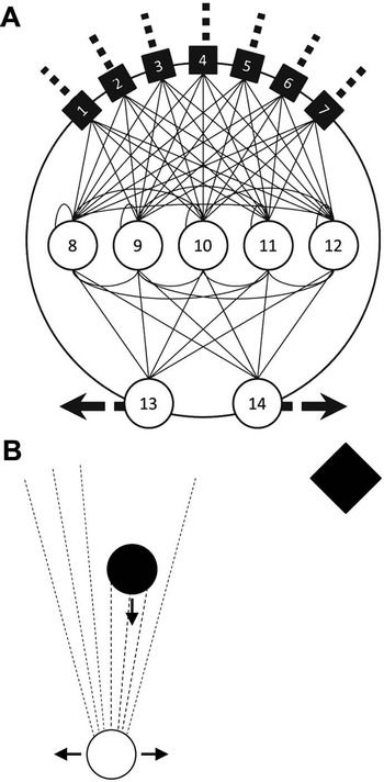
As a second example, consider Randall Beer's (Reference Beer2003) dynamical explanation of perceptual categorization in a simulated brain-body-environment system (fig. 2). The simulated system consists of a single minimally cognitive agent, equipped with a 14-neuron continuous-time recurrent neural network (CTRNN) brain and situated in a simple two-dimensional environment that features a single circular or diamond-shaped object. A 16-dimensional dynamical model defines the system's behavior:

Figure 2

The simulated agent, (A) its continuous-time neural network brain, and (B) its task environment. Figures adapted from Beer (Reference Beer2003).

Equations (1)–(16) define the change over time in the brain's neural activity (s ₁ … s ₁₄), the agent's horizontal position (x), and the object's vertical position (y). Neural parameters w, τ, σ, and are predetermined by an artificial evolutionary process and remain constant during as well as between trials. In contrast, the brain's neural activity is continuously affected by the changing sensory input vector I, a function of shape parameter α and of the relative positions of agent and object. Over the course of a single trial, a circular or diamond-shaped object falls vertically toward the agent, to which the agent responds by moving horizontally to catch circles and avoid diamonds, thus performing a categorical discrimination. Notably, discrimination is always preceded by an episode of active scanning: as the object falls, the agent repeatedly moves from side to side before eventually settling on a position either directly beneath the object or away to one side. Because this active-scanning behavior is an unexpected result of the artificial evolutionary process and cannot be straightforwardly read off the equations of the dynamical model, it constitutes a target phenomenon of significant explanatory interest.

Beer's goal is to use the tools and concepts of dynamical systems theory to explain how the observed active-scanning behavior (and thus, perceptual categorization) arises from the brain-body-environment system defined by the equations of the dynamical model. To this end, he adopts a clearly stated decompositional strategy: “We will decompose the agent-environment dynamics into: (1) the effect that the relative positions of the object and the agent have on the agent's motion; (2) the effect that the agent's motion has on the relative positions of the object and the agent” (Beer Reference Beer2003, 228; see also Beer Reference Beer1995).

This brief statement requires elaboration. In dynamical terms, equations (1)–(16) define a dynamical system composed of the simulated agent, its CTRNN brain, and the falling object. This dynamical system is mathematically equivalent to a pair of coupled dynamical systems (henceforth labeled “B” and “E”) defined by equations (1)–(14) and (15)–(16), respectively. Whereas B is a model of the embodied CTRNN brain that transforms sensory input into motor output, E is a model of the environment in which motor output is converted into sensory input. The couplings between B and E are defined by variables s₁₃ and s₁₄ in equation (14) and x and y in equations (1)–(7) and are best understood as a model of the two-way interface—the agent's body—that mediates between the brain and the environment. On this interpretation, Beer's aim is to show how the phenomenon of active scanning arises from the simultaneous and coupled activity of the embodied brain on the one hand and of the environment on the other.

At the heart of Beer's dynamical explanation lies a dynamical analysis that describes the activity of each of the two components—embodied brain and environment—identified above. This analysis comes in the form of a pair of steady state velocity fields and superimposed motion trajectories (fig. 3). The steady state velocity fields (colored regions) describe E's effect on the qualitative behavior of B—how the sensory input received at a particular position (x, y) constrains , the agent's horizontal velocity. The motion trajectories (colored lines) describe B's effect on the state of E—how causes a change in x and thus a change in the environment defined by (x, y).

Figure 3

Steady state velocity fields with superimposed motion trajectories for circle trials (left; “catch”) and diamond trials (right; “avoid”). Axes designate the relative positions of agent (x) and object (y), which together define the state of the environment. Colored regions describe the effect of the environment on the qualitative behavior (steady state velocity) of the embodied brain: blue indicates a steady state velocity directed toward the object; red indicates a steady state velocity directed away from the object; green designates a steady state velocity that may go in either direction. Colored lines correspond to a sampling of recorded motion trajectories several starting locations. Their color indicates the agent's instantaneous horizontal velocity according to the same color scheme as above, their shape indicates the way the relative positions of object and agent change over time, thus determining the agent's sensory input. Figure courtesy of Beer (Reference Beer2003).

The motion trajectories are superimposed on the steady state velocity fields in order to describe the spatiotemporal organization of embodied brain and environment. Of particular importance is the way the motion trajectories overshoot some colored regions while performing reversals over others. What determines whether a particular motion trajectory performs an overshoot or a reversal is the color of the region over which it is moving, as well as the amount of time it spends in that region. Specifically, a motion trajectory of a particular color (red or blue) performs a reversal whenever it is situated over a region of the opposite color and remains in it long enough for the agent's instantaneous horizontal velocity to approach the steady state velocity indicated by that region's color (red indicates velocities directed away from the object; blue indicates velocities directed toward the object).Footnote ⁶ Because active scanning is nothing but a particular combination of overshoots and reversals, it is explained by the particular details—shape and color—of the motion trajectories and steady state velocity fields in figure 3. That is, perceptual categorization via active scanning arises from the detailed ways in which B converts sensory input into motor output and E allows motor output to feed back on sensory input.

Although this discussion provides merely a rough sketch of Beer's dynamical explanation of perceptual categorization via active scanning (but see sec. 5.2 below), it suffices to show that the explanation is mechanistic in nature. First, Beer relies on the explanatory heuristic of structural decomposition to identify two working parts—the embodied brain on the one hand and the environment on the other—of a two-component mechanism realized in the simulated brain-body-environment system. Then, he provides a detailed dynamical analysis to describe the operations associated with each part—the way the embodied brain's steady state constrains motion in the environment and the way that motion affects the embodied brain's steady state at every possible relative position of agent and object. Finally, Beer describes the mechanism's spatiotemporal organization by discussing the detailed relationships between steady state velocity fields and motion trajectories that lead to overshoots and reversals. In summary, therefore, Beer describes the component parts, component operations, and organization of a mechanism for perceptual categorization via active scanning.Footnote ⁷

One additional feature of Beer's dynamical explanation is worth highlighting. Although the mechanistic explanation of perceptual categorization via active scanning is contained in his description of the mechanism composed of B and E, the behavior of at least one of those components affords further explanation. Why does the embodied brain behave the way it does in response to changes in the environment? Beer answers this question by describing the contributions of individual neurons in the agent's CTRNN brain. To this end, he provides separate steady state velocity fields for interneurons s ₈, s ₉, s ₁₁, and s ₁₂ (fig. 4) and shows that their sum is approximately equivalent to the steady state velocity field on the left side of figure 3.Footnote ⁸ That is, he describes a neural-level mechanism to explain the behavior of one of the two components of the agent-level mechanism responsible for active scanning.Footnote ⁹ In this sense, Beer's explanation is hierarchical in a way that closely resembles mechanistic explanations in other scientific domains; the components of a mechanism at one level of organization are further decomposed and explained in terms of mechanisms at lower levels of organization (Machamer et al. Reference Machamer, Darden and Craver2000; Craver Reference Craver2007; Bechtel Reference Bechtel2008).

Figure 4

Steady state velocity fields for interneurons 1–4 of the agent's CTRNN “brain.” Axes and coloring schemes as in figure 3. The color at any (x, y) in each of the four fields indicates the corresponding interneuron's contribution to the agent's steady state horizontal velocity during circle (“catch”) trials. Summing these four interneuron steady state velocity fields yields a steady state velocity field that closely resembles the one on the left side of figure 3. Figure courtesy of Beer (Reference Beer2003).

It is time to take stock. Thelen et al. (Reference Thelen, Schöner, Scheier and Smith2001) and Beer (Reference Beer2003) each offer a dynamical explanation of a (minimally) cognitive phenomenon. In each case, the explanation proceeds by identifying the component parts and operations of a mechanism and by showing how the organized activity of these parts and operations produces the phenomenon being explained. Therefore, Thelen et al. and Beer each provide a counterexample to the received view of dynamical explanation: some dynamical explanations are mechanistic explanations rather than covering-law explanations.

5. Cognitive Mechanisms: Extended and Complex?

Section 4 shows that dynamical cognitive science sometimes seeks the description of cognitive mechanisms. In this sense, many branches of dynamical cognitive science resemble computationalist and connectionist cognitive science as discussed in section 2. Although this may appear disappointingly conservative to the more radical proponents of dynamicism, I do not intend to deny that dynamicism is interestingly novel and important. Indeed, I agree with the popular assessment that dynamicist researchers are far more willing and able than some of their traditional colleagues to account for cognitive phenomena that arise from complex reciprocal interactions between brain, body, and the environment (for discussion, see Thelen and Smith Reference Thelen and Smith1994; Beer Reference Beer1995, Reference Beer2003; Kelso Reference Kelso1995; van Gelder Reference van Gelder1995, Reference van Gelder1998; van Gelder and Port Reference Port and van Gelder1995; Clark Reference Clark1997; Chemero and Silberstein Reference Chemero and Silberstein2008; Chemero Reference Chemero2009). Nevertheless, in this section I argue that this willingness and ability does not follow from a rejection of mechanistic explanation but from the invocation of the mathematical tools and concepts of dynamical systems theory. Indeed, a closer look at the dynamical explanations introduced in section 4 will show that the extant philosophical conception of mechanistic explanation may be underestimating the degree to which cognitive scientists are able to describe increasingly complex and distributed cognitive mechanisms.

6. Conclusion

Dynamical explanation is undeniably novel and important. As has already been argued elsewhere (e.g., Elman Reference Elman1991; Thelen and Smith Reference Thelen and Smith1994; van Gelder and Port Reference Port and van Gelder1995; Bechtel and Abrahamsen Reference Bechtel and Abrahamsen2010), in addition to introducing a very different mathematical framework to the study of cognitive phenomena, dynamical explanations are able to offer new perspectives on the role of temporal structure in behavior and cognition. In section 5, I argued that dynamical explanations are also uniquely well suited for dealing with continuous reciprocal causation and with interactions between brain, body, and the environment. As it happens, although in some well-known cases these explanations specify principles or laws, in other cases they describe the component parts, operations, and organization of mechanisms. Therefore, contrary to the received view, some dynamical explanations are mechanistic explanations rather than covering-law explanations. Moreover, contrary to the extant philosophical conception of mechanistic explanation, cognitive science may after all be in a position to describe mechanisms that exhibit continuous reciprocal causation and whose components span the boundaries between brain, body, and the environment.

In closing, it is worth noting some of the broader conceptual ramifications of the claim that some dynamical explanations are mechanistic in nature. First, mechanistic explanation is a form of reductive explanation; phenomena manifested at one level of organization are explained in terms of component parts and operations at lower level(s) of organization (Machamer et al. Reference Machamer, Darden and Craver2000; Craver Reference Craver2007; Bechtel Reference Bechtel2008). Because some dynamical explanations are mechanistic explanations, dynamical cognitive science is not as thoroughly antireductionist as many early proponents of dynamicism have claimed (see, e.g., Thelen and Smith Reference Thelen and Smith1994; Kelso Reference Kelso1995; van Gelder Reference van Gelder1998). Rather than being solely interested in identifying the principles that govern behavior and cognition at the “highest relevant level of causal organization” (van Gelder Reference van Gelder and Port1998, 622), dynamicist researchers seem equally interested in questions concerning the ways in which such regularities result from structures and processes at lower levels of organization.

Second, those dynamicist researchers who seek to provide mechanistic explanations rather than covering-law explanations may be steering toward reconciliation with proponents of representationalism. By describing cognitive mechanisms rather than principles or laws, these researchers describe structures that are amenable to what Chemero and Silberstein (Reference Chemero and Silberstein2008) have called representation hunting—characterizing the components of a mechanism as representation producers and representation consumers and understanding their operations in terms of the transfer and manipulation of information. Notably, episodes of representation hunting have already occurred both for Beer's dynamical agent (Ward and Ward Reference Ward and Ward2009) and for Thelen et al.'s dynamical field theory model (Spencer and Schöner Reference Spencer and Schöner2003). Although true reconciliation between dynamicism and representationalism will be possible only if a suitable notion of representation can be articulated—one that accommodates the emphasis on temporal structure, continuity, and physical distribution distinctive of dynamical cognitive science—the search for such a notion is very likely to be intriguing.