Due to the relative scarcity of more direct measures, the quality of medieval English harvests are typically inferred from grain prices. Persistence—protracted runs above and below trend—is a well-known property of pre-industrial grain price series. Beveridge (Reference Beveridge1922, p. 452) argued that “periodicities in the weather” produced runs in the harvest and thus grain prices. Hoskins (Reference Hoskins1968, p. 17) hypothesized that grain prices persisted not due to “weather-cycles but to the underlying factor of yield-ratios.” Since England “was an agrarian economy that worked on a very fine margin between bread-corn and seed-corn,” in “very bad years the rural population must have staved off the worst of their hunger by consuming part of next year’s seed-corn.” This linked harvests year to year as one “bad harvest tended to generate another because of a scarcity of seed corn and so cumulatively until a fundamental change in the weather-pattern in a given year broke the downward sequence and restored the ‘normal’ balance between bread-corn and seed-corn” (Hoskins Reference Hoskins1968, p. 17). The modern literature rejects both Beveridge and Hoskins, finding that the annual harvest was “self-contained”—randomly distributed around a mean independent of any previous harvest.Footnote 1 In this view, runs in grain prices do not reflect persistent harvests but persistent markets linked intertemporally through grain stores.
I present evidence that both good and bad harvests persisted. Specifically—controlling for contemporaneous covariates—in years following a failed harvest: (i) yields per acre and per seed are 15–20 percent lower; (ii) the variance of yields per acre and per seed is 40–50 percent lower; and, (iii) the probability of a subsequent harvest failure is 20–30 percent higher. Three empirical innovations relative to the literature help explain my divergent findings: (i) yields are not aggregated but instead analyzed as a balanced panel by year, manor,Footnote 2 and crop; (ii) only subperiods with continuous annual observations are analyzed; and, (iii) tests for persistence are made relative to a subsistence standard not relative to trend. My sample exhibits low spatial correlation so that aggregating yields over groups of manors reduces both the variance and persistence of the harvest. So while the hypothesis that manorial harvests were self-contained annual events is rejected, broader harvest measures, depending on how they aggregate regional grain supplies, may display different dynamics. Thus, a version of the “Hoskins hypothesis,” properly formulated and applied, is an important complement—not a substitute—to existing theories of harvest and price persistence.
Understanding the temporal and spatial nature of harvest shocks is fundamental to the literature on peasant consumption risk.Footnote 3 Fafchamps (Reference Fafchamps1999, p. 2) distinguishes between three types of risks faced by peasant farmers: “high and low frequency risks; autocorrelated and non-autocorrelated risks; and collective and idiosyncratic risks.” Large infrequent shocks that persist are among the most difficult to manage, “If shocks persist, coping is more difficult…Identifying the nature of the shock helps identify the possibilities for dealing with its consequences” (Dercon Reference Dercon2002, p. 143). Finding significant autocorrelation in the medieval harvest thus has important implications for the efficacy of alternative risk coping strategies available to peasant households. Grain stores are relatively effective as a consumption smoothing device, but less so in the presence of temporally correlated shocks.Footnote 4 When the spatial correlation of shocks is low, sharing arrangements may provide relatively more effective insurance. Income sharing, however, suffers from high agency costs, limiting its ability to pool harvest realizations over spatially heterogeneous regions. For a typical peasant household a failed harvest constituted a significant source of both contemporaneous and future subsistence risk; a source of risk that was especially difficult to insure against. To the extent that large persistent harvest shocks stressed traditional consumption smoothing mechanisms, many peasant households, especially small-holders, would be pushed into land markets as sellers. Dyer (Reference Dyer1989) argues land sales driven by harvest risk produced a dynamic that tended to increasingly concentrate land amongst largeholders. Bekar and Reed (Reference Bekar and Reed2013, p. 19) find that distress sales of small parcels during harvest failures contributed to the dramatic increase in measured wealth inequality and poverty over the twelfth and thirteenth centuries, “more households found themselves increasingly vulnerable to distress land sales as they worked ever smaller holdings. Many of these small- and middleholder families eventually found themselves landless. This dynamic created a sequence of increasingly unequal landholdings and poverty over time.”
The reliability and consistency of grain prices as a proxy for the annual harvest relies crucially on the assumption that harvests were self-contained events. Fogel (Reference Fogel, Higonnet, Landes and Rosovsky1991, p. 37) notes that grain prices reflect current harvest conditions alone only under “the implicit assumption that the annual supply of grains varied directly with the annual per acre yield. That assumption would be correct only if carryover inventories at the beginning of the harvest were zero.” Also crucial in these calculations is the demand for seed corn, the largest component of retained grain aside from consumption requirements. Wrigley (Reference Wrigley, Walter and Schofield1989, p. 243) notes that in order to use annual grain prices as a proxy for the harvest it is important, “that the quantity of grain used as seed-corn did not vary from year to year whatever the scale of the previous harvest…since, at the levels of yield under discussion, this would be in many cases the weightiest element in deciding the matter…” When sow rates are constant, and harvests independent, the gross harvest is perfectly correlated with the marketable harvest. This in turn implies that the price elasticity of grain can be estimated from contemporaneous price and yield data alone, rendering grain prices a good proxy for subsistence risk. The finding of significant autocorrelation in harvests renders each of these conclusions potentially problematic. If households exercised significant discretion over “fixed” overhead grain requirements—that is, if sow rates and other charges varied year to year—the gross and net harvests will be imperfectly correlated, grain prices a potentially biased proxy of subsistence risk, and elasticity estimates may need correction.
These two examples—given the centrality of the harvest to the pre-industrial economy—could be multiplied. The nature of harvest risk has been linked to peasant mortality, credit market activity, fertility decisions, labor market activity, and more. For those using yields to study the productivity of medieval agriculture, my findings suggest something akin to a “rational expectations” result. The annual harvest was not solely a function of contemporaneous covariates but also past household decisions; yields are not an exogenous primitive reflecting soil quality, labor inputs, and weather shocks alone, but are instead endogenous to a history of decisions embodying information regarding household expectations over production, consumption, and risk.
SEED CORN AND SOW RATES
That sow rates displayed considerable variation among regions, estates, and manors is well documented. In his study of Norfolk, Campbell (Reference Campbell1983, p. 388) finds that sow rates “conformed to local practice and the practice was subject to wide variation within the area. The effect of the variation when combined with that already identified in yield per seed is therefore to produce marked contrasts in yield per acre, particularly where high seeding rates coincided with high yield ratios.” Mate (Reference Mate1985, pp. 25–26) notes that “Lay and ecclesiastical lords, with estates scattered in different parts of the country, adopted different seeding rates in each area.” Kent enjoyed relatively high yields per acre due in part to high sowing rates “yet they made no effort to increase seeding rates outside of Kent.” Brandon (Reference Brandon1972) and Campbell (Reference Campbell1983) document a range of managerial strategies relying on varying sow rates to maximize and stabilize harvests by trading off yields per seed and per acre. For example, on small parcels heavy manuring or greater labor inputs could offset otherwise lower yields associated with thinner seeding. In regions where heavy soil was hard to prepare or susceptible to invasive weeds, increased seeding densities served as a substitute for labor.Footnote 5 Brandon (Reference Brandon1972, p. 410) finds that “the simple device of altering seeding rates” was not always the product of arbitrary norms or customs but instead deliberately implemented to “regulate grain production, within relatively narrow limits…”
In some regions a relative scarcity of seed corn may have consistently constrained agricultural productivity, “low seedings on many English manors were well below the optimum for the growing conditions then prevailing for the maximum potential yield. Thus low seedings (unless exceptional manuring was practiced) presumably reflect the large element of ‘natural economy’ prevalent in the Middle Ages” (Brandon Reference Brandon1972, pp. 408–9).Footnote 6 In extreme cases a shortage of seed corn could substantially alter the balance between the farmed and unfarmed arable (with the latter given over to pasture or planted as grass). In his study of the fourteenth century reversion of the arable, Baker (Reference Baker1966, p. 530) found that “The Nonarum Inquisitiones also suggest that the reversion of arable land and the dereliction of many messuages were closely associated with impoverished and shrinking populations and with shortages of seed corn” and that in “Ivinghoe more than 400 acres lay neglected partly because the parishioners were impoverished, having neither animals for ploughing nor seed for sowing; and at Great Missenden 200 acres lay in a similar condition and for a similar reason.”
There is much evidence that harvest failures pushed small- and middle-holders to consume seed corn. This evidence is consistent with peasant budget studies. For households farming 15 acres in 1300, Dyer (Reference Dyer1989, p. 113, table 7) finds the net wheat harvest for sale or carryover was just seven bushels. Given their fixed expenditures, a 10 percent decline in wheat yields might push the household to economize on consumption and/or seed. A household farming a standard holding would face the same tradeoff after a 20 percent decline. Kitsikopoulos (Reference Kitsikopoulos2000) calculates that a household farming a standard virgate (30 acres) produced a gross wheat harvest of 66 bushels per year. This left a net harvest of 43 bushels after deducting tithe and seed corn. The fixed overhead of the tithe, seed corn, and manorial charges was greater in relative terms for middle- and small-holders. Surveying the literature on the distribution of the arable in pre-plague England suggests that up to 50 percent of the peasant population farmed a middle-holding or less and that, therefore, “a sizable proportion of the English peasantry faced a liquidity problem on a quasi-permanent basis which could not always be resolved by borrowing” (Kitsikopoulos Reference Kitsikopoulos2000, p. 251).Footnote 7
Both Kitsikopoulos and Bailey note that peasants struggling with debt and harvest failure often resorted to land market sales. Peasants pushed into the land market as sellers were often caught in a downward spiral, with their shrinking land holdings putting their household at ever more risk, and “if land was being sold to pay off debts or purchase food, then it seems certain that tools, utensils, seed corn, and livestock were also sold or consumed” (Bailey Reference Bailey1998, p. 241). Razi (Reference Razi1980, p. 152) notes, “The reason for the rapid quickening of the inter-peasant land market during periods of economic crises is that smallholders and to a lesser extent half yardlanders had to sub-let and to sell land either to remit debts or to pay rents and fines to buy food, seed corn and livestock.”Footnote 8
The gross harvests of large-holders were more substantial, and, for similar fixed charges, their net harvests proportionately larger; they would expect to face shortages in their net harvest less frequently. Regardless, those farming a standard virgrate, landlords, and even estate managers, were not wholly free from shortages of seed corn. Throughout the mid-fourteenth century the officers of Battle Abbey and Ramsey Abbey faced a series of difficult tradeoffs regarding crop mix and acres planted as a result of falling revenues. Mate (Reference Mate1984, p. 343) finds that on these manors it was not just weather conditions or crop disease that pushed manorial officers to reduce their plantings but “lack of seed corn as well as…the lack of workers.” During roughly the same period, at Bourchier Hall in Essex, Britnell (Reference Britnell1977, p. 61) finds that poor quality seed corn resulted in harvest failure and that “there was less grain on the manor than was needed even for its own use in seed, fodder and stipends, and the serjeant had to lay out sums of up to £15 a year on grain purchased from elsewhere.” In his analysis of the same accounts, Long (Reference Long1979, p. 459) notes that falling yields and deficient harvests were caused by poor, not exhausted, soil along with the debility of its seed, which “is probably a reference either to the poor quality of the seed (bladum debile), or to the poor yield of the crop (propter debilitatem),” terms “frequently encountered in documents of the time.” Following repeated failed harvests starting in 1647, a report to Parliament noted a widespread lack of seed corn amongst the population of Cumberland, “The committees and justices of the peace of Cumberland certified ‘that there were 30,000 families that had neither bread nor seed corn, nor money to buy either, and they desired a collection for them, but much too little to relieve so great a multitude’ ” (Hindle Reference Hindle2008, p. 69). Mate (Reference Mate1984, p. 343) notes that in mid-fourteenth century Lawling, with drought impacting the Christ Church manors, “the serjeant frequently spent large sums on the purchase of grain for seed and to give to the famuli….” That manorial officers were consistently looking to supplement their supplies of seed corn is consistent with Gras’ analysis of early grain markets. Gras documented extensive markets in seed corn based on regional clusters of closely situated manors. While the most important grain trade involved rural manors and major urban centers, the next most important involved “a constant transfer of corn from one manor to another…The corn so sent was either ad semen or ad opus, for seed purposes or to meet a deficiency of crops or supply with an adjoining manor of the group” (Gras Reference Gras1926, p. 7).
Other factors interacted with sow rates to link yields year to year. Wrigley (Reference Wrigley, Walter and Schofield1989, p. 240) notes that fodder supplies “fluctuate from year to year according to the scale of the preceding harvest. But they could not be altered substantially without penalty in the subsequent harvest since the amount of useful work obtainable from draught animals was strongly affected by both the quantity and type of fodder given to them.” This was true of labor inputs as well. In Sussex, after excessive rains produced spring flooding, Cooper (Reference Cooper2006, pp. 105–6) found a failed harvest in 1339 impacted the next year’s harvest in two ways, “First, people had obviously been driven so far as to eat their precious stock of seed corn…people faced the grim choice between starving now or eating into the seed corn and putting next year’s crop at risk” and, second, “people were too weak to deal properly with the spring planting of 1340.” Britnell (Reference Britnell1977) finds that poor harvests could reduce the quality of seed corn and soil preparation in the following year. Finding a “grouping of bad years” in his data, Osmaston (Reference Osmaston1985, p. 499) posits that it may be “due to the ‘knock-on’ effect of one bad harvest—bad seed for the next sowing and debilitated labour and draught animals—rather than a similar causal factor, perhaps weather, in each year of the group,” concluding it may “therefore be wrong to treat such years as independent variables.” Appleby (Reference Appleby1979, p. 869) notes that “In times of crisis, smallholders might be forced to eat their seedcorn. And the weather that damaged one harvest might extend into the preparation for the next; for example, a very late harvest could delay the planting of the next crop…”Footnote 9 Baker (Reference Baker1966, pp. 530–31) notes, “When a harvest failed wholly or partially, whatever the reason, there was less seed available for sowing in the following agricultural year and the arable acreage contracted. Again, when a harvest failed both peasants and livestock might die of hunger or at least have their effectiveness impaired by undernourishment, and with fewer and weaker beasts for ploughing and fewer and weaker hands to hold the plough and tend to the crops, the arable acreage might have diminished still further.”
PEASANT ALLOCATIONS AND THE HARVEST
I develop a simple model in which harvests vary with sow rates and a vector of complementary inputs.Footnote 10 Agents allocate their annual harvest, net of customary and other fixed charges, between seed corn, bread corn, and stored corn. A binding subsistence constraint implies that poor harvests may persist.
Consider an autarkic, infinite-horizon, agricultural economy in which agents derive all of their real income (measured in grain) from farming a fraction (l t ≥ 0 acres) of a fixed land endowment L. In each period (t), agents allocate their gross harvest—the current period’s realized harvest (H t) plus depreciated carryover (δS t−1)—between grain consumed as calories (C t = c tH t), retained for seed (K t = k tH t), spent on other inputs (V t = v tH t), retained as carryover (S t = s tH t), or paid as customary charges (τ). Agents face a subsistence constraint ( $\underline{C}$); subsistence events are not “catastrophic” but increase the incidence of distress, disease, and other chronic challenges to household health and welfare. Consumed grain produces utility in the current period,
 $$U\left( {{C_t}} \right) = \left\{ {\matrix{ {u({C_t})} \hfill & {if} \hfill & {{C_t} \ge \underline{C}} \hfill \cr 0 \hfill & {if} \hfill & {{C_t} \lt \underline{C}} \hfill } } \right.$$
The function u(·)is a standard utility specification (with u′ > 0, u″ < 0, and u′ → ∞ as  ${C_t} \to \underline{C}$). Sown grain yields σ = {0 … ∞} quarters of grain per seed where the yield function is: (i) increasing in sow rates per acre (κ =K/l) up to a maximum sow rate (κ max) beyond which yields are either constant or falling;Footnote 11 (ii) increasing in a vector of complementary inputs (V); (iii) shifted by exogenous weather shocks (ω); and, (iv) shifted by exogenous productivity shocks (ε) which are assumed to be normally distributed around zero.Footnote 12 Formally,
 $${\sigma _t}\left( {{\kappa _{t - 1}},{V_{t - 1}},{\omega _t},{\varepsilon _t}} \right)with\left\{ {\matrix{{{{\partial \sigma } \over {\partial {\kappa _{t - 1}}}} \gt 0,{{{\partial ^2}\sigma } \over {\partial \kappa _{t - 1}^2}} \lt 0if{\kappa _{t - 1}} \le {\kappa _{\max }}} \cr {{{\partial \sigma } \over {\partial {\kappa _{t - 1}}}} \le 0,{{{\partial ^2}\sigma } \over {\partial \kappa _{t - 1}^2}} \ge 0if{\kappa _{t - 1}} \gt {\kappa _{\max }}}} } \right. .$$
Agents are assumed to solve the following problem,
 $$\begin{array}{l} \mathop {\max }\limits_{{c_t},{k_t},{v_t},{l_t}} {E_0}\mathop \sum \limits_{t = 0}^\infty {\beta ^t}U\left( {{c_t}{H_t}} \right)\\ s.t.{c_t}{H_t} \le {\sigma _{t - 1}}{k_{t - 1}}{H_{t - 1}} + \delta {s_{t - 1}}{H_{t - 1}} - {k_t}{H_t} - {v_t}{H_t} - {s_t}{H_t} - \tau \end{array}$$
Solving Equation (1) produces sequences of decisions for: consumption  $\{ c_t^\ast\} _{t = 0}^\infty $, seed planted
 $\{ k_t^\ast\} _{t = 0}^\infty $, input use
 $\{ v_t^\ast\} _{t = 0}^\infty $, and acres planted
 $\{ l_t^\ast\} _{t = 0}^\infty $. The first three determine carryover
 $\{ s_t^\ast\} _{t = 0}^\infty $, the second and fourth sow rates per acre
 $\{ \kappa _t^\ast\} _{t = 0}^\infty $. I assume the return on sown seed combined with costly medieval storage would lead peasants to choose
 $k_t^\ast \ge {k_{max}}$ in a normal harvest year. For a given planted acreage in period t, substituting the optimal shares into the budget constraint and setting τ = 0 implies,
 $${\sigma _{t - 1}}{K_{t - 1}} = \left( {c_t^* + s_t^\ast + k_t^\ast + v_t^\ast} \right){H_t} - \delta s_{t - 1}^\ast{H_{t - 1}}.$$
In any period  $c_t^\ast + s_t^\ast + k_t^\ast + v_t^\ast = 1$, so Equation (2) reduces to σ t−1 = H t − δS t−1/K t−1. Assuming zero stores, and that k, v, and l are constant, σ t = H t /K (in terms of yield per acre, σ tK/l). The reduced form of Equation (2) contains no lagged terms, meaning contemporaneous grain prices are a consistent proxy for self-contained harvests.Footnote 13 Relaxing these assumptions implies that harvests may be linked in three ways. A failed harvest may cause agents to: (i) consume a portion of their seed corn reducing both k t and κ t; (ii) reduce their planted acreage (l t); and/or, (iii) reduce and/or alter the mix of complementary inputs (V t). Put another way, agents may act on: (i) the intensive margin, farming the same number of acres less intensively (decreasing per acre sow rates and manuring); and/or (ii) the extensive margin, farming fewer acres (maintaining per acre sow rates and manuring). Operating on the intensive margin would tend to reduce the size of the harvest and yields per acre; operating on the extensive margin would tend to reduce the size of the harvest while possibly maintaining yields per acre.Footnote 14 To account for these possibilities I test for the persistence of yields per acre and per seed.
Whether harvests are self-contained depends on the sequence of harvests and how agents substitute between consumption, storage, and seed during poor harvests: (i) Good harvests (H g) occur when an agent’s net harvest allows them to consume at subsistence and implement optimal sow rates (k ≥ k*) without impacting the supply of other harvest inputs ( ${H_g} + \delta {S_{t - 1}} - \underline{C} - {S_t} - {\rm{\tau }} \gt K_t^\ast + V_t^\ast$); (ii) Scarce harvests (H s) occur when an agent’s net harvest allows them to consume at subsistence but unable to implement optimal sow rates (k < k*) or apply the necessary mix of complementary inputs (
 ${H_s} + S{\delta _{t - 1}} - \underline{C} - {\rm{\tau }} \lt K_t^\ast + V_t^\ast$); and, (iii) Failed harvests (H f) occur when an agent’s net harvest does not allow them to consume at subsistence (
 ${H_f} + \delta {S_{t - 1}} - \tau \lt \underline{C}$). So, while harvests below trend may or may not persist, scarce and failed harvests will tend to persist.Footnote 15 Thus, in contrast to the existing literature—which tests for persistence relative to deviations from moving trends—I test for persistence relative to a subsistence target.
DATA AND EMPIRICAL STRATEGY
The standard measure of harvest persistence is the degree of autocorrelation in aggregate yield series (typically a weighted average of yields over a large collection of manors and/or vills).Footnote 16 Analyzing nineteenth-century French data, Wrigley (Reference Wrigley, Walter and Schofield1989, pp. 244–45) finds that harvests were distributed randomly and independently: “The die was thrown afresh each year and the result of the cast was not biased by the throw of the previous year. If the quantity of corn retained for seed did vary with the scale of the harvest, it was not enough to influence the yield in the following year systematically, even to the limited extent of keeping it on the same side of the average yield.” Working with a wider sample (including English, French, and Belgian yield data from the thirteenth through nineteenth centuries), Nielsen (Reference Nielsen1997, pp. 17–18) first confirms Wrigley’s findings for England in the late medieval period and then generalizes his findings over most of English history, “From the middle ages to modern times the results are consistent. The annual shocks to harvests appeared as random events. Serial correlation of prices resulted not from correlated harvests, but from the smoothing effects of forward-looking storage on total supply.” I argue that this approach has at least four important limitations: (i) it relies on aggregate series, smoothing observed yields and suppressing the proposed causal linkage between harvests at the level of the manor; (ii) it relies on interpolation for years with no data; (iii) it is not clear why harvests below trend should persist; and, (iv) the tests involve analyzing simple correlations without controlling for potentially important covariates.
My unit of observation is the annual yield per seed and per acre on individual manors. The data is taken from Titow’s (Reference Titow1972) study of the Winchester Estates.Footnote 17 I do not interpolate over breaks in the data, analyzing six distinct subperiods with continuous annual series (1268–1274, 1283–1292, 1297–1302, 1306–1318, 1325–1332, 1335–1349) as strongly balanced panels sorted by manor and crop. Quoted in quarters, the yield data is summarized in Table A1 in the Appendix.Footnote 18 Drawn exclusively from the wealthy manors of the Winchester Estates, covering the thirteenth-century through to the early years of the Black Death, this is not a “random sample” of English yields. Possible sources of bias in my panel stem from its relative lack of temporal, geographic, and manorial diversity. Despite their geographic concentration, the manors of Winchester display significant heterogeneity, covering a range of soil types, husbandry, and managerial strategies. Another issue concerns the management of the estates. Overseen by the Bishop of Winchester, one might expect a centralized effort to smooth the geographically idiosyncratic shocks over the manors of the estate. Instead the manors display a persistent heterogeneity in management styles, the importance of demesne farming, crop mix, market integration, and so on.Footnote 19
The Winchester pipe rolls are relatively unique in their completeness, rendering its manorial yield data a standard source in a range of literatures related to the harvest.Footnote 20 The Winchester rolls allow an almost unique opportunity to study a series of unbroken observations at the manorial level, necessary for a theoretically consistent and empirically meaningful test of persistence. I therefore follow Nielsen (Reference Nielsen1997, p. 14) in noting that while “the lack of suitable production data from the early modern period makes a direct test difficult…Medieval manorial data provide an opportunity to examine the patterns of grain output and prices in a period arguably more enlightening of the early modern English situation.”
The Persistence of Failed Harvests, Autocorrelation in Yields
The conclusion that harvests were self-contained rests on three related findings: (i) yield aggregates strongly regress to trend; (ii) yield aggregates do not display significant autocorrelation; and, (iii) yield aggregates do not display excessive runs. A key parameter for all of the empirical exercises that follow concerns what constitutes a “scarce harvest.” Consistent with the literature, I define yields 85 percent or more below the mean as a scarce harvest.Footnote 21
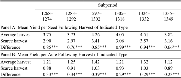
In my sample there is no subperiod in which aggregate yields are systematically lower following scarce harvests; they are consistently lower, however, at the level of the manor. Table 1 reports mean yields for manors having experienced a scarce harvest in the previous period relative to those experiencing an average harvest in the previous period. In each case, the hypothesis that mean yields following a bad harvest are the same as those following an average harvest is rejected.
MEAN WHEAT YIELDS BY LAGGED HARVEST TYPE

* = Significant at the 5 percent level.
** = Significant at the 1 percent level.
*** = Significant at the .01 percent level.
Notes: Average harvest calculated as mean wheat yield over those manors that experienced a harvest within 85 percent of its mean in the previous period. Scarce harvest calculated as mean wheat yield over those manors experiencing a harvest less than 85 percent of its mean in the previous period.
Sources: For Panels A and B yield data taken from Titow (Reference Titow1972).
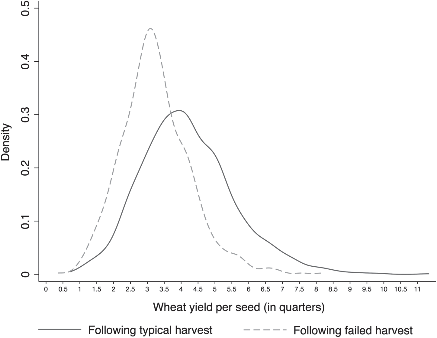
Relatedly, Figure 1 plots the frequency density functions for yields in years following scarce harvests and those following average harvests (taken over the entire sample). Consistent with the means test, a scarce harvest in t − 1 shifts and truncates the distribution lowering its mean in period t.Footnote 22
KERNEL DENSITY PLOT OF WHEAT YIELDS PER SEED

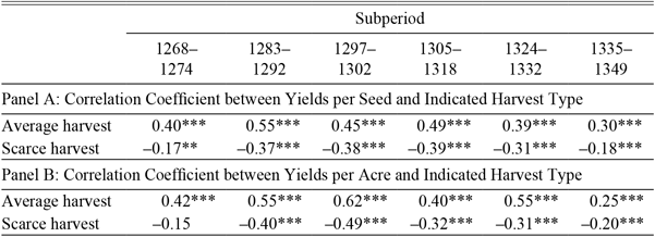
Nielsen (Reference Nielsen1997, p. 15) suggests that a “more formal test of the relationship examines the autocorrelation coefficient of the yield series, which when yields are defined as ratios and thus detrended is simply the correlation between the ratio in each year with that of its successor.” Self-contained harvests imply that this ratio should display no autocorrelation, which I again confirm for the harvest aggregate. However, both yields per acre and per seed display authocorrelation in my panel. Calculating the correlation between yields and harvest type, I find: (i) a positive correlation between yields and lagged yields following average harvests; and, (ii) a negative correlation between yields and lagged yields following scarce harvests. Table 2 reports the correlation coefficient between yields and lagged yields by harvest quality.
CORRELATION COEFFICIENT BETWEEN SUCCESSIVE YIELDS BY HARVEST TYPE

* = Significant at the 5 percent level.
** = Significant at the 1 percent level.
*** = Significant at the .05 percent level.
Notes: Average harvest calculated as correlation coefficient between current yield and yield in the previous period for manors experiencing a harvest within 85 percent of its mean in the previous period. Scarce harvest calculated as correlation coefficient between current yield and yield in the previous period for manors experiencing a harvest less than 85 percent of its mean in the previous period.
Sources: For Panels A and B yield data taken from Titow (Reference Titow1972).
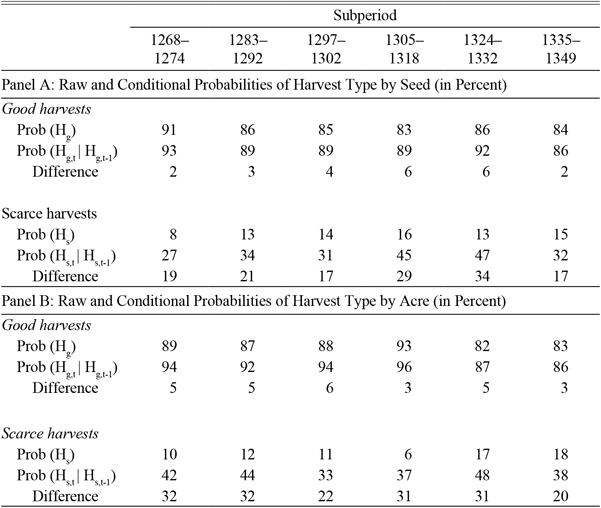
Another indication that poor harvests persist is their relative frequency. Both Wrigley and Nielsen find that yields displayed too few runs and were therefore random. I again confirm their findings for the harvest aggregate: a runs test fails to reject the hypothesis that aggregate yields were a random sequence, but the same test rejects the hypothesis that manorial yields were random. Consider a related measure, the information content of the current harvest. Like stocks on a random walk, self-contained harvests provide no information about future harvests. If harvests are random the conditional probability that next year’s harvest will fail is simply equal to the unconditional probability that any harvest will fail. Persistent harvests, on the other hand, do provide information about future harvests. More formally, letting Hg = good harvest and Hs = scarce harvest: (i) if harvests are self-contained, then Prob(Hg,t|Hg,t−1) = Prob(Hg), and Prob(Hs,t|Hs,t−1) = Prob(Hs); and (ii) if harvests persist, then Prob(Hg,t|Hg,t−1) > Prob(Hg) and Prob(Hs,t|Hs,t−1) > Prob(Hs). Table 3 reports a summary of the probabilities by period for yields per seed.
CONDITIONAL AND UNCONDITIONAL PROBABILITY OF HARVEST TYPE

Notes: Probability of a good/scarce harvest calculated as frequency of good/scarce harvests over entire sample. Probability of good/scarce harvest conditional on good/scarce harvest calculated as frequency of harvest type given the type of harvest in the previous year. Probability of good and scarce harvests may not always sum to 100 percent due to rounding.
Sources: Yield data taken from Titow (Reference Titow1972).
Consistent with correlated harvests, manors experiencing a good harvest have a higher conditional probability of experiencing a subsequent good harvest than would be expected randomly; manors experiencing a scarce harvest have a higher conditional probability of experiencing a subsequent failed harvest than would be expected randomly.Footnote 23
MODELING THE HARVEST
The correlations analyzed to this point suggest that harvests persisted at the level of the manor. To control for the possibility that the observed correlations result from the persistence of unobserved covariates—like Beveridge’s cyclical weather patterns—I estimate a model of following form,
 $$yiel{d_{m,t}} = {\alpha _m} + {\beta _1}scarc{e_{m,t - 1}} + {\beta _2}fodde{r_{m,t - 1}} + {\omega _i}climat{e_t} + {\nu _j}mano{r_{m,t}} + {\tau _1}year + \varepsilon ,$$
where, (i) yield m,t is yield per acre or per seed for manor m in period t; (ii) scarce m,t−1 is a lagged dummy equal to 1 if the wheat harvest was less than 85 percent of the mean in the previous period on manor m; (iii) fodder m,t−1 is a lagged dummy equal to 1 if the barley and oats harvest were jointly less than 85 percent of the mean in the previous period on manor m; (iv) climate t is a vector of weather controls in period t common to all manors; (v) manor m,t is a vector of manor-level controls in period t; and (vi) year is a time trend starting in 1211. Comparative static predictions on the variables of interest are derived from the model: (i) a scarce harvest in period t − 1 implies a trade-off between retained seed corn, consumption, and the possible supply of complementary inputs (β 1 < 0); and, (ii) a failed fodder crop in period t − 1 reduces the supply of complementary inputs shifting the yield curve downwards (β 2 < 0).
The Winchester Estates faced declining yields over the sample period. Fitting mean yields by manor against time suggests a negative trend for yield per acre and a weak trend for yield per seed. Further, testing for year fixed effects suggests that they are not jointly zero and a simple OLS specification of yields against time produces a small but significant negative coefficient. Since annual dummies control less for trends and more for idiosyncratic harvest conditions, I include both a time trend and a set of annual dummies. The model includes two other sets of controls: climatological and manorial. My final list of controls includes proxies for temperature and precipitation shocks, animals per acre, distance from London, manorial husbandry, manorial farm type, manorial soil type, and a time trend. The construction of the controls—and a summary of the data presented in Table A1—is described in the Appendix.
Estimation Results
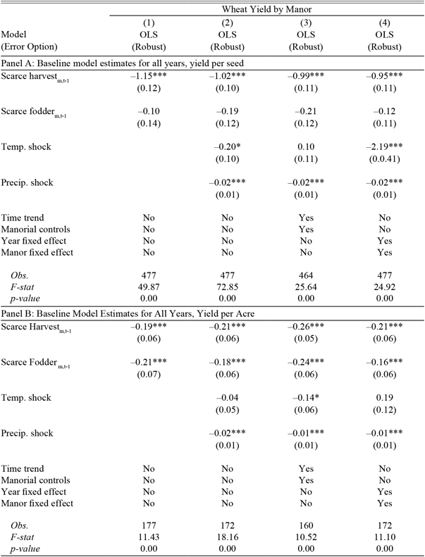
The initial estimates are presented for a restricted sample (1305–1318) in Table 4. Column (1) presents an estimate of the baseline specification with no controls; Column (2) with climatic controls alone; Column (3) with a time trend and my constructed controls. Finally, Column (4) presents an OLS estimate with climatic controls along with year and manor fixed effects. As mentioned, the panel displays some heteroscedasticity, all specifications are therefore estimated with robust errors. Panel (A) reports yield per seed, panel (B) yield per acre.
BASELINE SPECIFICATION ESTIMATES, WHEAT (1305–1318)

* = Significant at the 5 percent level.
** = Significant at the 1 percent level.
*** = Significant at the .05 percent level.
Notes: Column (1) presents OLS estimates for Equation (3) from text, no controls included. Column (2) presents OLS estimates for Equation (3) from text with climate controls included. Column (3) presents OLS estimates for Equation (3) from text with time invariant manorial controls and time trend. Column (4) presents OLS estimates for Equation (3) with climate controls, year fixed effects, and manor fixed effects. Robust errors are specified in each case.
Sources: For Panels A and B yield data taken from Titow (Reference Titow1972).
The coefficients of interest both take their predicted signs: (i) a failed harvest in t − 1 reduces yields per seed and per acre in t; (ii) a failed fodder harvest in period t − 1 also reduces yields in period t. A warm weather shock tended to increase yields, too much or too little rain tended to reduce yields. The estimates and diagnostics are consistent across the specifications. While each of the models is well specified, and produce similar estimates, I adopt Column (4) as my preferred specification. In Specification (3) most of the constructed controls and the time trend are either insignificant or their estimated coefficients extremely small. On the other hand, in Column (4) both the year and manor fixed effects—which control for unobserved covariates not captured in my controls—are sizable and mostly significant. The specification in Column (4) also has the benefit of simplicity, placing the least structure on the functional form of either the shared controls or idiosyncratic shocks.
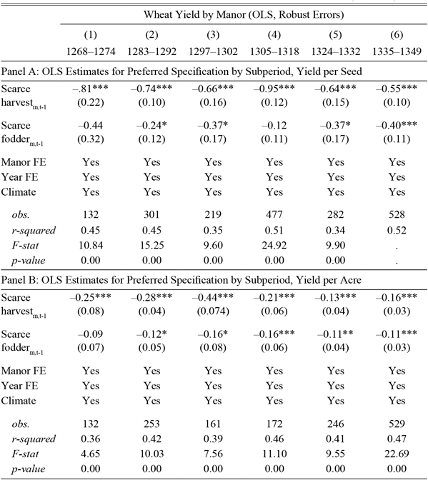
The data over the period 1211–1349 includes missing years (the pipe rolls skip from 1211 to 1218 for example). Interpolating missing years mechanically imposes regularity between observed yields and missing yields introducing a bias towards finding persistence where none exists. To control for this interpolation bias I estimate the preferred specification for each subperiod in the sample with continuous years of observation. The results are presented in Table 5.
PREFERRED SPECIFICATION OLS ESTIMATES BY SUBPERIOD (WHEAT)

* = Significant at the 5 percent level.
** = Significant at the 1 percent level.
*** = Significant at the .05 percent level.
Notes: Columns (1)–(6) presents OLS estimates for Equation (3) from text with climate controls, year fixed effect and manor fixed effect for each subperiod with annual contiguous observations. Robust error option specified in each case.
Sources: For Panels A and B yield data taken from Titow (Reference Titow1972).
The estimated coefficients are consistent with the model’s predictions in each subperiod. In each subperiod the effect of a failed harvest is statistically significant; a failed fodder crop is statistically significant in roughly 80 percent of the cases. The results are strongly consistent with the raw correlations presented in Tables 1–3. A key parameter in my analysis is the level of a scarce harvest. Table 5 assumes, consistent with the literature, that a scarce harvest occurs when a harvest is equal to or less than 85 percent of the mean harvest. To test the robustness of the results to varying cutoffs I estimate the preferred specification where scarce harvests are defined as 90, 80, 75, 70, and 60 percent, respectively, of the mean harvest.Footnote 24 The results are presented in Table 6.
ROBUSTNESS OF ESTIMATES TO LEVEL OF SCARCE HARVEST (WHEAT)

* = Significant at the 5 percent level.
** = Significant at the 1 percent level.
*** = Significant at the .05 percent level.
Notes: Columns (1)–(6) presents OLS estimates for Equation (3) from text with climate controls, year fixed effect and manor fixed effect for each subperiod with annual contiguous observations. Scarce harvest is defined as a varying percentage of the harvest as indicated in the first column. Robust error option specified in each case.
Sources: For Panels A and B yield data taken from Titow (Reference Titow1972).
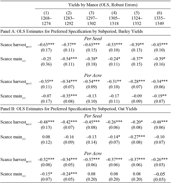
Consider the behavior of the other main food crops, oats and barley. Table 7 replicates the estimates from Table 5 for barley and oat yields by subperiod. All of the controls and diagnostics are the same as Table 5. The only difference is that instead of controlling for a failed fodder crop I control for a failure of the other main food crops. I define a failed food crop as a situation in which the wheat and oat yields or wheat and barley yields are jointly below 85 percent of their mean.
PREFERRED SPECIFICATION BY SUBPERIOD, BARLEY AND OATS

* = Significant at the 5 percent level.
** = Significant at the 1 percent level.
*** = Significant at the .05 percent level.
Notes: Columns (1)–(6) presents OLS estimates for Equation (3) from text with climate controls, year fixed effect and manor fixed effect for each subperiod with annual contiguous observations. Robust error option specified in each case.
Sources: For Panels A and B yield data taken from Titow (Reference Titow1972).
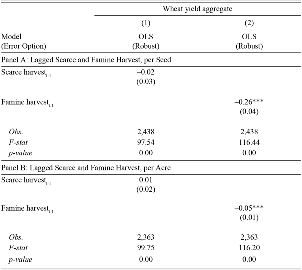
To test the hypothesis that the use of aggregate yield series obscures harvest persistence by smoothing harvest shocks across manors, I run the preferred specification of Equation (3) with an aggregate yield series. The comparative static predictions for the variables of interest in this specification are different from the baseline specification: when the independent variable is manorial yields (yield m,t) I predict β 1, β 2 < 0; when the independent variable is aggregate yields (yield t) I predict β 1 = β 2 = 0. Visually inspecting mean yields per seed and per acre reveals the relative rarity of aggregate harvest failure. To capture large and/or spatially correlated shocks I define a “famine” harvest as a year in which mean yields fell below one per acre or three per seed. This definition captures two well-known historical famines in the sample (the famines of 1218 and 1315) along with a few other dramatic crop failures. All of the standard manorial, climatic, and time controls are included. The results are shown in Table 8.
ESTIMATES FOR YIELD AGGREGATE (WHEAT)

* = Significant at the 5 percent level.
** = Significant at the 1 percent level.
*** = Significant at the .05 percent level.
Notes: Column (1) presents the estimated persistence coefficient on a scarce harvest, a harvest less than 85 percent of the mean, for the yield aggregate. Column (2) presents the estimated persistence coefficient on a famine harvest—a yield per seed less than 3, a yield per acre less than 1—for the yield aggregate.
Sources: For Panels A and B yield data taken from Titow (Reference Titow1972).
While scarce harvests persisted at the level of the manor, they did not persist at the level of the Winchester Estate; widespread spatially correlated famine harvests persisted for both. Notably, when estimated with aggregate yields I find that shocks common to all manors in the sample (e.g., weather) are still significant and have the correct sign. The low spatial correlation of harvests, controlling for common weather shocks, suggests that regional markets in seed corn were imperfect.
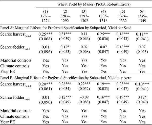
Table 3 indicates that a failed harvest increased the probability of a subsequent harvest failure by 150 ~ 400 percent (the probability of future harvest failure conditioned on the current harvest having failed ranged from 33 to 38 percent while the unconditional probability of future harvest failure ranged from 6 to 18 percent). To estimate this probability while controlling for other covariates, I present a probit specification of Equation (3). Instead of presenting the estimated coefficients from the probit regressions I calculate their marginal effects and present the results of this second step in Table 9. The coefficients represent the marginal contribution of the variable to the probability of a failed harvest in the current period.
MARGINAL EFFECTS OF HARVEST FAILURE, BY SUBPERIOD (WHEAT)

* = Significant at the 5 percent level.
** = Significant at the 1 percent level.
*** = Significant at the .05 percent level.
Notes: Columns (1)–(6) presents the marginal effects for variables of interest. Marginal effects are derived from a Probit regression of Equation (3) from text, all controls included, for each subperiod with annual contiguous data exists. Robust error option specified in each case.
Sources: For Panels A and B yield data taken from Titow (Reference Titow1972).
Consistent with the measured decline in the mean and variance of yields following a scarce harvest, a harvest shortfall in period t − 1 increases the probability of experiencing a failed harvest in period t in a statistically and economically significant manner.
Discussion and Implications
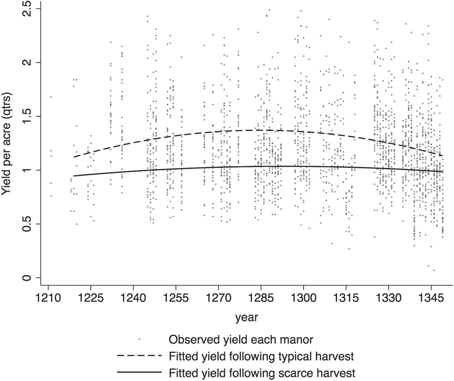
It is illuminating to map the impact of a failed harvest onto a middle-holder’s consumption risk. Figure 2 presents a quadratic best fit for yields following good and scarce harvests against a scatter of yields over all manors. The effect of a failed harvest appears reasonably constant over the period.
FITTED YIELDS PER ACRE FOLLOWING GOOD AND SCARCE HARVEST

While the raw correlations and regression coefficients do not distinguish between the three mechanisms linking harvests, yields are asymmetrical in a manner consistent with a concave yield function and the importance of varying sow rates.Footnote 25 Defining a “good harvest” symmetrically to a scarce harvest—yields at least 15 percent above the mean—I note that mean yield per acre is 1.20 quarters for the entire sample, 1.28 quarters conditional on the previous harvest being good, and 0.98 quarters conditional on the previous harvest being scarce. In other words, a good harvest increased yields by half as much as a failed harvest reduced them (a roughly 6 percent increase relative to a roughly 18 percent decrease). Consider a stylized illustration of a peasant household farming 30 acres (with 15 fallow or to clover, 5 to barley, 5 to oats and peas, and 5 to wheat). In a typical year their harvest would be around six quarters of wheat, after a failed harvest around five quarters. Assuming that 15 percent of the harvest is set aside for the tithe and other manorial transfers, and two bushels for seed, a failed harvest alone—assuming all other shocks “zero out”—implies a 28 percent reduction in the household’s net wheat harvest in a year following a failed harvest.Footnote 26 The effect is proportionally larger for middle-holders, and much more dramatic for small-holders. This admittedly rough estimate suggests that a failed harvest may have constituted one of the most serious sources of intertemporal consumption risk in the medieval agricultural economy.
One does not have to reject a Hoskins-effect or the persistence of harvests in order to establish that grain stores were the source of price runs. My empirical results suggest that the persistence in grain prices is related to, but not wholly determined by, the persistence of the harvest. Grain prices are determined in regional markets by the joint supply decisions of geographically linked manors, vills, and/or households. The strength of the link from harvest persistence to price persistence is thus a function of how regional markets served to aggregate individual manorial harvests and the degree of spatial correlation between those harvests. For example, if the Winchester Estates constituted an integrated grain market the link would be extremely weak for the region as a whole. Yields across the individual manors in the sample were only weakly correlated in a typical year, in the first subperiod (1268–1274) the coefficient of variation for aggregate wheat yields is 0.13, for manorial yields it is 0.30. This implies a correlation coefficient between yields over the 38 manors of just 0.01. In this case only very large shocks, and/or spatially correlated shocks, would produce persistence in harvest aggregates and therefore grain prices.
CONCLUSION
Each step in my analysis suggests that harvests were not self-contained—that both scarce and good harvests persisted. The differences in means from Table 1, along with the regression coefficients from Table 5, present consistent estimates for the size of the effect. Taking a simple weighted average of the differences from Table 1, controlling for no other covariates, suggests that a scarce harvest lowered subsequent yields by roughly 25 percent per acre or 21 percent per seed; controlling for potential covariates, Table 5 indicates that the effect was roughly 20 percent per seed and per acre. Not only do mean yields fall following a scarce harvest, but they are more tightly clustered around that lower mean (the standard deviation of yields following a bad harvest falls from 0.42 to 0.28, see Figure 2). This combination of a lower mean and variance implies a significantly higher likelihood of a subsistence event following a scarce harvest. Here the raw correlations suggest a larger effect than do the marginal effects derived from the probit analysis. Looking at the probabilities from Table 2 alone suggests that a failed harvest more than doubled the risk that the next harvest would fail. On the other hand, a weighted average of the marginal effects from Table 6 suggests that the marginal contribution of a failed harvest to subsequent harvest failure is between 20–30 percent, suggesting that harvest failure was not the sole source of persistence.Footnote 27
By reducing the mean and variance of subsequent harvests, a failed harvest represented a major source of intertemporal consumption risk to peasant households. Yield aggregates display persistence only for especially dramatic famine events, and/or periods when it is known from the historical record that weather shocks repeated. This suggests that the intertemporal risk from harvest failure was mostly localized and that the distribution of shocks faced by peasant households displayed a higher level of temporal autocorrelation relative to spatial correlation than is suggested by the existing literature. Understanding the temporal and spatial makeup of the medieval harvest is an important input into evaluating the efficacy of different risk coping strategies available to peasant households. Taken together, my two main findings suggest, for example, that sharing arrangements and grain purchases/sales may have been relatively more effective at lowering the variance in consumption relative to income than were grain stores.Footnote 28 Findings from the modern development literature suggest a more speculative possibility, in the presence of risk and incomplete asset markets peasant households may have engaged in forward looking strategic behavior regarding their seed corn. Anticipating planting shocks may have led agents to alter their planting strategies or even hold precautionary stores of seed. Rather than representing an exogenous fixed overhead charge, seed corn stores would be endogenous to past harvests, contemporaneous planting conditions, and peasant beliefs about future harvest shocks.
Appendix
Appendix 1: Data Description/Summary, Construction of Controls
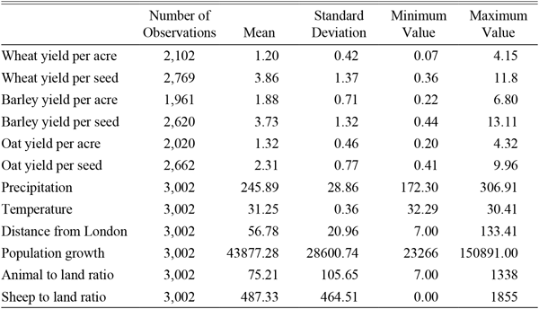
Table A1 summarizes the data used to create Tables 1–9 in the text.
SUMMARY STATISTICS FOR ENTIRE DATA SET

Notes: Yields are quoted in quarters per acre/seed. Titow (Reference Titow1972, p. 82) simply reports no data if there is any doubt whether customary or perch acres were used. I treat such entries as missing. This is only an issue on 6 of 38 manors, and in only one of the subperiods (1283–1292). I analyze six distinct subperiods with continuous annual series (1268–1274, 1283–1292, 1297–1302, 1306–1318, 1325–1332, 1335–1349). The precipitation series is taken from tree ring data collected in East Anglia. Cooper et al. (Reference Cooper, Thomas, Tyers, Wilson and Keith2012) construct the series to analyze precipitation in south central England. I produce a series of spliced 30-year trends; shocks are then calculated by differencing annual observations from the 30-year trend. The temperature series is taken from measures of sea surface temperatures in the northern hemisphere. Sicre et al. (Reference Sicre, Ian, Mignot, Myriam Khodri, Minh-Xuan, Eirksson and Luise Knudsen2011) constructed the original series to analyze northern European climatic shifts. I produce a series of spliced 30-year trends. Temperature shocks are then calculated by differencing annual observations from the 30-year trend. Population growth measures the change in the population of each manor. Specifically, it is calculated as the difference between a manor’s population level at the time of the Hundred Rolls and Domesday survey. Measures the animals (cows and ox primarily) divided by the acreage of the manor. Measures the sheep on a manor divided by the acreage of the manor.
Sources: Wheat, barley, and oat yield data is sampled from Titow (Reference Titow1972) which reports yields from 41 manors. I drop Calbourne, Brightstone, and East Meon Church due to the number of missing observations. The data is transformed into a strongly balanced panel sorted on year (1268–1349) and manor. Distance: Derived from longitude and latitude data. Population growth: Data on population is taken from Broadberry, Campbell, and Leeuwen (Reference Broadberry, Bruce and van Leeuwen2010). Animal and sheep: Data is taken from Titow (Reference Titow1972).
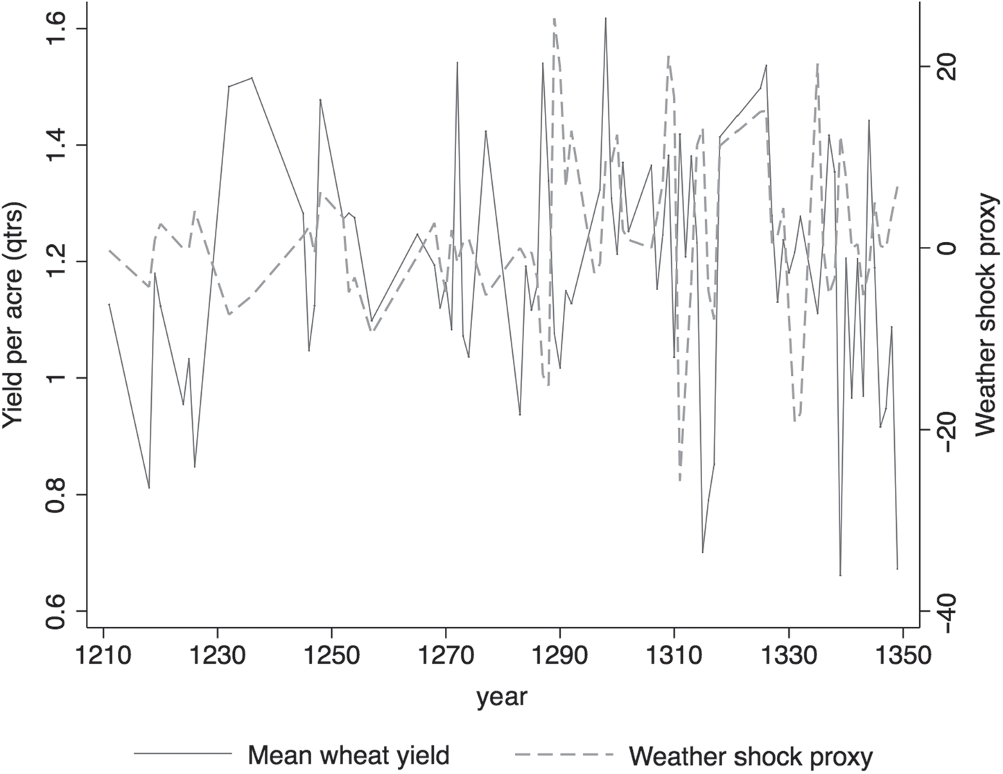
Medieval agriculture was sensitive to weather, lacking modern methods of irrigation, drainage, fertilizer, and so on. Considered in terms of its effect on harvests, climate can be usefully summarized as a combination of temperature and precipitation (see Titow Reference Titow1961). Consistent with a large literature,Footnote 29 Schneider’s (Reference Schneider2011) factor analysis of 19 possible proxies underlying English climate extracts three heavily weighted factors: two proxy temperature and the last correlates strongly with rainfall. The effect of precipitation on harvests was asymmetric. Excessive precipitation in the summer and fall produced the worst growing conditions (especially when combined with cold weather); extreme drought could be problematic, but dry weather was less of an issue and often led to relatively good harvests. Titow (Reference Titow1960, p. 363) finds that “outstandingly good harvests” tended to follow dry winters/summers while “outstandingly bad harvests” followed very wet autumns/summers. In sum, good harvests tended to result from: (i) a warm growing season (especially in summer and early fall); and (ii) steady average rainfall (too little or too much rain could both be bad for the harvest). To proxy temperature I employ historical measures of sea surface temperatures in the northern hemisphere. The data is taken from Sicre et al. (Reference Sicre, Ian, Mignot, Myriam Khodri, Minh-Xuan, Eirksson and Luise Knudsen2011, p. 1) who produce a “time series of sea surface temperatures spanning the last two millennia…by combining a proxy record from a new sediment sequence with previously published data.” The time series is used to analyze medieval climatic shifts in the northern hemisphere. The series is calibrated against modern temperature data and consistently benchmarks the warming of the “Medieval Climatic Anomaly” and the later cooling of the “Little Ice Age.” The sequence of temperature shocks is produced by differencing the current period’s temperature from a 30-year moving trend. To proxy rainfall I employ historical estimates of precipitation from models based on tree-ring data from East Anglia. The observations are taken from Cooper et al. (Reference Cooper, Thomas, Tyers, Wilson and Keith2012, p. 1019) who use tree-ring data from oaks to produce an “annually resolved reconstruction of spring-summer precipitation in East Anglia, UK for the period AD 900-2009.” This overlaps the Winchester Estates significantly and was chosen since it “falls neatly within the central England coherent precipitation region…where relatively spatially homogeneous precipitation is expected across all sites” (Cooper et al. Reference Cooper, Thomas, Tyers, Wilson and Keith2012, p. 1020). The model is calibrated against observed rainfall and tree growth in the modern period and explains between 30 to 35 percent of the annual variation in regional rainfall. The sequence of precipitation shocks is produced by differencing the current period’s precipitation from a 30-year trend. Since my climatic controls are constructed as deviations from a 30-year trend, errors in either series—whether produced by the climate models and/or measurement issues—are significantly smoothed by differencing.Footnote 30 In Figure A1 I interact the temperature and precipitation shocks to produce a “weather” series, plotting it against mean wheat yields over the entire sample. The correlation coefficient between the weather series and yields is negative and significant (⍴ = –0.174, significant at the 1 percent level).
WEATHER PROXY AND ANNUAL MEAN WHEAT YIELDS

Two sets of manorial controls are included.Footnote 31 The first control for idiosyncratic differences between manors assumed to be constant over the sample. The most important of these relate to a manor’s soil quality and type. Taking from Campbell’s (Reference Campbell2000) classification of English manors, I include dummies for each manor’s crop mix, soil type, farm type, and husbandry strategies. Urban manors, especially those proximate to London’s large commercial grain markets, may have been relatively more productive and/or sensitive to market conditions. To proxy this effect, I control for a manor’s distance from London in miles. Finally, I include a series of county dummies for each manor. The second set of controls capture idiosyncratic differences between manors. Malthusian population dynamics suggest that, all else equal, more productive manors should support higher population densities. I use Broadberry, Campbell, and Leeuwen (Reference Broadberry, Bruce and van Leeuwen2010) to construct a “population difference” series which measures the change in each manor’s population density per. I also control for animal inputs per acre (primarily horses and oxen) and the importance of sheep husbandry on each manor (both measured as a ratio of the relevant animal(s) per acre on the manor). In no form of the model, in any subperiod, or for any crop type, were the county dummies, sheep per acre, population growth, or crop type controls individually or jointly significant.