


List of Symbols

1. Introduction
One of the main challenges in glaciological sciences is understanding glacier dynamics, in terms of mass and thermal flows, basal processes and responses to climate change. Many authors have faced the problem of describing ice dynamics through numerical modelling. Most of the large-scale ice-sheet models are based on the shallow-ice approximation (SIA) which, by assuming a small aspect ratio between vertical and horizontal dimensions of the domain, neglects part of the stresses and considers the pressure hydrostatic. After the original work of Reference MahaffyMahaffy (1976), a number of models have been proposed and applied to studying ice-sheet dynamics (Reference JenssenJenssen, 1977; Reference HuybrechtsHuybrechts 1990; Reference GreveGreve, 1997; Reference Ritz, Fabre and LetréguillyRitz and others, 1997; Reference Calov, Savvin, Greve, Hansen and HutterCalov and others, 1998). SIA models have also been used to study the motion field in valley glaciers (Reference Hubbard, Blatter, Nienow, Mair and HubbardHubbard and others, 1998; Le Reference Le Meur and VincentMeur and Vincent, 2003). The hypothesis of a small aspect ratio, on which the SIA relies, may fail on medium- and small-scale applications. A way to improve these models is represented by the higher-order models in which second-order stresses are considered (Reference GudmundssonGudmundsson, 1997a, Reference Gudmundssonb; Reference Colinge and BlatterColinge and Blatter, 1998; Reference PattynPattyn, 2002). A two-dimensional method, in which the equations are integrated line by line over the ice depth in order to compute the basal conditions, is proposed by Van der Reference Van der VeenVeen (1989) and Van der Reference Van der VeenVeen and Whillans (1989). A two-dimensional ice-sheet model in which a projection method is used for the time-advancing scheme and classical second-order finite-difference formulae are used for the space discretization is presented by Reference Mangeney, Califano and HutterMangeney and others (1997). Commercial finite-element codes have also been used for modelling ice dynamics (Reference GudmundssonGudmundsson, 1999; Reference Lüthi and FunkLüthi and Funk, 2000, Reference Lüthi and Funk2001). Some finite-difference time-advancing schemes are presented and compared in Reference Greve and CalovGreve and Calov (2002). A recent work (Reference Martín, Navarro, Otero, Cuadrado and CorcueraMartín and others, 2004) includes a complete treatment of the pressure field.
The target of the present work is the implementation of a general three-dimensional method capable of working on large- and small-scale applications. For this reason a fluid-dynamic approach has been considered and a method capable of modelling the full stress and pressure fields is presented. The full pressure field is computed by splitting the pressure into hydrostatic and hydrodynamic components (Reference CasulliCasulli, 1999; Reference Casulli and ZanolliCasulli and Zanolli, 2002). It should be noticed that no stress component is neglected in the proposed method. The use of fully three-dimensional equations requires the imposition of boundary conditions on all the domain boundaries, not only on surface and bedrock as usually done in SIA and higher-order models thanks to the small-aspect-ratio hypothesis. The model is based on the Stokes equations and the Saint-Venant equation which are discretized in space by means of the finite-volume method in order to guarantee both local and global mass and momentum conservation. High-order approximations are used for the discretization of equations and boundary conditions. The equations are discretized in time by a modified projection method that can take the free-surface time evolution into account.
The paper is organized as follows: In section 2 the governing equations are presented. In section 3 the space and time discretization of these equations is presented together with the description of the boundary conditions. For clarity, in this section only the time semi-discretization of the field equations is presented; the space- and time-discretized equations and the formulae for the approximation of the derivatives are given in Appendices A and B, respectively. In section 4 three theoretical applications are presented and in section 5 the model is applied to the real case of Priestley Glacier, Antarctica. Finally in section 6 some conclusions are drawn.
2. Governing Equations
Following the approach proposed by Reference NyeNye (1952) and commonly accepted and used in glaciological studies, ice is a non-Newtonian viscous fluid, governed by the Navier–Stokes equations. If a meso- or large-scale model is investigated, then convective terms are negligible since they act on a much smaller space- and timescale (Reference Colinge and BlatterColinge and Blatter, 1998);however, when small-scale phenomena are to be investigated (frontal movements, crevasse opening, etc.), convective terms might be retained. In what follows, the unsteady Stokes equations for an incompressible fluid will be considered; the equations written in conservation form are:


where u =[u, v, w]T is the three-dimensional velocity vector, t is the time, ∇. Is the divergence operator, ∇ is the gradient operator, ν is the kinematic viscosity, p = tr(σ)/3ρ is the kinematic pressure and g is the gravity acceleration vector. The strain-rate tensor is represented by

For temperate ice masses, when large- or mesoscale applications are investigated, the term ∂ u/∂t can be neglected, the only transient development being surface evolution. In these cases the time derivative can be used to numerically solve Equations (1) and (2) until a steady state is reached (Reference Mangeney, Califano and HutterMangeney and others, 1997).
The momentum equation (1) can be written as

so that the momentum equation for the single velocity components can be solved separately. The term ∇ · [ν(∇u)] will be called the ‘diffusive term’.
Ice viscosity is described by the following relation derived from Glen’s law:
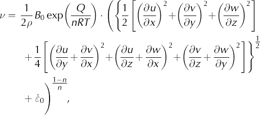
where B
0 is the viscosity parameter, Q is the activation energy for creep, R is the perfect gas constant, T is the temperature, n is the exponent in Glen’s law and  is a small number (e.g. 10−30 a−1) used to avoid singular behaviour where the stress vanishes.
The surface of an ice mass is a stress-free surface that can evolve in time. The surface evolution can be caused by changes in the inner motion field as well as by changes in the accumulation/ablation rate. Denoting the surface elevation above an undisturbed reference level by s, the kinematic boundary condition for the free surface is

where a s is the accumulation/ablation rate at the surface multiplied by the modulus of the gradient of the free surface function (|∇S| = |(∂s/∂x, ∂s/∂y, – 1)T|). Denoting the depth of the bedrock with respect to the undisturbed reference level by –b, the kinematic boundary condition for the ice/bedrock interface is

where a (–b) is the basal melting/refreezing rate multiplied by the modulus of the bedrock gradient.
Integration of the incompressibility equation (2) from the bedrock to the surface and substitution of Equations (5) and (6) lead to the Saint-Venant equation:

where a = as – a (–b). This equation describes the free surface evolution in time as a function of the unit-discharges and incorporates the physical law of mass conservation.
3. Numerics
3.1. Space discretization
A solution in closed form for the unsteady three-dimensional Stokes problem is not known, even in simple cases; thus an approximated solution has to be computed by numerical methods. Conservation of mass and momentum is crucial for the stability and the accuracy of the solution, especially in the presence of a moving boundary such as the free surface (Reference Deponti, Pennati, de Biase, Sundén, Brebbia and MendesDeponti and others, 2004). The finite-volume method is used for the discretization of the field equations since it guarantees both local and global conservation of mass and momentum.
An undisturbed reference level s 0 coincident with the linear least-squares approximation of the physical surface is considered. In the reference system used, the x-y plane lies on s 0, the x axis is oriented along the mean flow direction and points downhill, the z axis points upward and the y axis is consequently determined. The domain is partitioned by means of cell-centred control volumes in the shape of rectangular prisms (Fig. 1);each control volume face is orthogonal to one coordinate axis, and the union of all the control volumes determines the computational domain. The dimensions of each control volume are Δx, Δy and Δz. The volume horizontal dimensions are chosen on the basis of a priori knowledge of the domain peculiarities and are fixed throughout computation. The volume height is also fixed with the same criterion for the volumes far from the free surface, but, due to its evolution, the height of those including the free surface can change in time and it may be necessary to add or suppress some volumes; this is why the dimension Δz will be time-indexed from now on. Control volumes filled with ice are called active.
Sketch of a three-dimensional control volume.

The field equations are integrated on each control volume; by the Green–Gauss theorem this leads to computing the surface integral of the flux of the diffusive terms (diffusive fluxes). These are calculated by summing the contributions of each control volume face, i.e. using the product of the representative value of the diffusive term and of the face area (integral mean value theorem). Hence, diffusive fluxes are to be approximated on each control volume face; this is done by a four-point centred differencing scheme (see Appendix B for details). The scheme is general enough to allow for non-uniform spacing between adjacent points and is third-order accurate. The volume integrals are approximated using the integral mean value theorem.
3.2. Time-advancing scheme
A method for time integration of Stokes equations without particular assumptions on the pressure field is the projection method (a particular type of fractional step method) in which the equations are integrated in two or more steps. This method is widely used in fluid dynamics, and many formulations have been proposed in the literature (e.g. Reference GreshoGresho, 1991; Reference Guermond and QuartapelleGuermond and Quartapelle, 1998; Reference Armfield and StreetArmfield and Street, 2002).
The projection method alone cannot describe the free surface evolution, and direct calculation of the kinematic boundary condition at the surface (Equation (5)) or of the Saint-Venant equation (7) may lead to physical inconsistency and to numerical instability. Indeed, the kinematic boundary condition and the Saint-Venant equation are to be computed on the basis of a velocity field consistent with the new surface elevation in spite of its being unknown; this could become important in the presence of accumulation/ablation or in the presence of varying dynamic boundary conditions at the surface. For these reasons, a modified projection method in which the Saint-Venant equation is kept in order to calculate the free-surface evolution is proposed in this work.
As mentioned in the Introduction, the pressure in an ice mass is not always hydrostatic; in particular, in the presence of bedrock perturbations or of changes in the basal sliding conditions a hydrodynamic pressure occurs. This phenomenon is also called the ‘bridging effect’ (Van der Reference Van der VeenVeen and Whillans, 1989; Reference Blatter, Clarke and ColingeBlatter and others, 1998). The total kinematic pressure, p, is divided into the hydrostatic part, |g|(s – z), and the hydrodynamic part, π,

In the first step, provisional velocities  are calculated by considering the contribution of the hydrostatic pressure at the preceding time-step, q, and neglecting the contribution of the hydrodynamic pressure:

where ∇Sq = (∂sq/∂x, ∂sq/∂y, –1)T is the gradient of the free surface function and the superscripts represent the time indices. The physical boundary conditions for the three velocity components are imposed on all boundaries. In the first step the incompressibility equation is not considered so that the provisional velocity field is, in general, nondivergence-free.
The target of the second step of the projection method is the formulation of a second-order equation for the total pressure or for a part of it, in which the mass conservation principle (expressed by the null-divergence constraint) is accounted for. In our formulation the second-order equation for the hydrodynamic pressure, π, is obtained by applying the divergence operator to the momentum equation written in the form

and considering the null-divergence constraint

This equation holds for the control volumes not connected to the surface. In the presence of a moving surface, the mass conservation and the compatibility between the velocity field and the surface geometry are guaranteed by a combination of the incompressibility equation (2) and the Saint-Venant equation (7). Hence, the discretized form of the equation for π at the surface control volumes is obtained by combining the discretized form of Equations (2) and (7) (Equation (A13) in Appendix A). The second-order discretized equation for π is thus given by the conjunction of the discretized form of Equation (11) (Equation (A8) in Appendix A) and the discretized equation at the surface (Equation (A13) in Appendix A). Homogeneous Neumann boundary conditions are imposed at all boundaries.
Once the hydrodynamic pressure is calculated, the final velocity field is computed by Equation (10); assuming the pressure to be hydrostatic only in the surface control volumes, the final free-surface elevation is computed by

The final velocity field is divergence-free since the mass conservation has been imposed in the second step; moreover the free-surface elevation is consistent with the inner velocity field since the Saint-Venant equation has been considered.
3.3. Boundary conditions
As said above, physical boundary conditions for the three components of the velocity field are applied at all boundaries in the first step, while homogeneous Neumann boundary conditions are imposed in the second step for the hydrodynamic pressure at all boundaries. Let us focus on the boundary conditions for the velocity field. At the open boundaries (inflow and outflow sections), homogeneous Neumann boundary conditions are applied. At the surface the stress-free condition applies. At lateral solid walls and at the bedrock the impenetrability condition holds for the normal velocity component, while a sliding condition is required for the tangential and binormal velocity components. The relation between basal stress and sliding velocity is expressed by

where u (−b) is the basal velocity vector, C is a sliding parameter and

is the basal stress vector, I being the identity matrix. The three-dimensional sliding relation (13) automatically satisfies the impenetrability condition expressed by Equation (6) where a (−b) = 0 (Reference HutterHutter, 1983). If C = 0 the relation translates into the no-slip condition, i.e. homogeneous Dirichlet; if C → ∞ the condition translates into the perfect slip condition, i.e. homogeneous Neumann. In all other cases the condition is a Robin boundary condition and allows the computation of stress and sliding velocity at the same time.
Numerical boundary conditions are approximated by means of high-order (second and third) generalized finite-difference formulae (presented in Appendix B); this yields a good approximation of the boundary conditions and allows for non-uniform volume dimensions. In particular, the control volumes can be smaller where a better accuracy of the solution is required.
4. Theoretical Applications
The applications presented in this section aim to evaluate the method performance and to investigate important aspects in ice dynamics such as the influence of viscosity on velocity and pressure fields, basal sliding and flow over undulating bedrocks. For these targets it is useful to consider theoretical tests in which the aspect being investigated can be emphasized; hence two-dimensional tests are considered. Even though the problems are two-dimensional, they are modelled in a complete three-dimensional setting where homogeneous Neumann conditions are imposed in the transverse direction (y direction). Results will be presented in vertical sections (x-z planes).
Steady-state solutions are calculated starting from an undisturbed situation; the time discretization is chosen on the basis of the desired accuracy and of the stability conditions imposed by the method. The iterations are stopped when the difference, δ, between two successive iterates is smaller than a fixed tolerance. This difference is computed on the whole domain by

where the i index describes the three velocity components and the j index extends to all control volumes.
4.1. Uniformly inclined plane
In the first application a section of an infinite slab is considered. Surface and bedrock are flat, parallel and inclined at a small angle (5°). The expected solution is the so-called ‘laminar flow regime’ (Reference NyeNye, 1952; Reference PatersonPaterson, 1994) in which the vertical and transverse velocity components are null and the free surface remains undisturbed. The domain is partitioned into 1575 control volumes (21 rows in the x direction, 25 in the z direction and 3 in the y direction), of which 1512 are active; the time-step, Δt, is 0.5 years. Iterations are stopped for δ ≤ 10−4. Different sliding parameters, ranging from the no-slip condition to the perfect slip condition, are tested. In all cases the velocity field agrees with the expected solution, the free surface remains undisturbed and the velocity divergence is null everywhere. Different constant values of the kinematic viscosity are tested.
In Figure 2 the vertical profile of the horizontal velocity component for the no-slip case is presented for three different kinematic viscosities: ν = 1011, 1012, 1013 m2 s−1. The number of iterations performed to reach the steady state were 508, 134 and 26 for the three viscosity values, respectively. The model sensitivity to viscosity changes can be appreciated. It can be seen that the lower the viscosity, the higher the surface velocity; since no-sliding conditions apply, for lower viscosity vertical deformations are larger.
Vertical profile of the longitudinal velocity for three kinematic viscosities: ν = 1011 m2 s−1 (solid line), ν = 1012 m2 s−1 (dashed line), ν = 1013 m2 s−1 (dotted line).

4.2. Variations in basal slipperiness
In the second application the influence of variations in basal slipperiness on pressure and velocity fields and, consequently, on the free-surface geometry are investigated. The proposed test is similar to the one presented in Reference Blatter, Clarke and ColingeBlatter and others (1998) and Reference Colinge and BlatterColinge and Blatter (1998): an infinite slab is considered but in this case the sliding parameter C varies locally. In particular, an 8 km long and 1 km deep domain is considered; the bedrock is inclined at 5° with respect to the horizontal direction. Perfect slip conditions are prescribed in a 1 km long central portion of the domain while no-slip conditions are prescribed elsewhere. The domain is partitioned into 3024 active control volumes (72 rows in the x direction, 14 in the z direction and 3 in the y direction); the time-step, Δt, is 0.5 years. Iterations are stopped for δ ≤ 10−4; a total of 470 iterations were performed to reach steady state.
In Figure 3 the results of the simulation with a constant kinematic viscosity ν = 1012 m2 s−1 are presented. In Figure 3a the velocity field is shown: it can be seen how, in the vicinity of the slipperiness variations, vertical velocities increase. These vertical velocities produce a perturbation of the free surface that can be appreciated in Figure 3b. The apparent positive local slope of the free surface (in this and in subsequent figures) is due to the inclined reference system adopted and to the differing vertical and horizontal scales. Finally, in Figure 3c the hydrodynamic pressure field is presented: it can be seen that in the presence of slipperiness variations the pressure field is not purely hydrostatic. Indeed, where the sliding conditions change from no-slip to perfect slip, a longitudinal extension (accompanied by negative hydrodynamic pressure) occurs while a longitudinal compression (accompanied by positive hydrodynamic pressure) occurs when the sliding conditions change from perfect slip to no-slip. As mentioned in section 3.2, this phenomenon is called the bridging effect. Even if the hydrodynamic pressure is about two orders of magnitude smaller than the total pressure, it is related to vertical velocities and surface perturbations. This test confirms the importance of a complete treatment of pressure and stress fields in the solution of the full Stokes problem.
(a) Velocity field, (b) free surface and (c) hydrodynamic pressure field of the flow in the presence of variations in basal slipperiness. The components of the gravity acceleration vector in the considered reference system are gx = 0.855, gy = 0.000, gz = −9.773 (see section 3.1). Negative and positive hydrodynamic pressures arise in the vicinity of slipperiness variations; these kinematic pressures are related to vertical velocities and free-surface perturbations. Note the different scales of horizontal and vertical axes.

4.3. Undulating bedrock
In the third application the influence of bedrock undulations on pressure and velocity fields and, consequently, on the free-surface geometry are investigated. Similar investigations have been performed by Reference GudmundssonGudmundsson (1997a, Reference Gudmundssonb, Reference Gudmundsson2003), Reference SchoofSchoof (2002) and Reference HindmarshHindmarsh (2004). In our simulation a 4 km long domain is considered. The mean domain thickness is 1 km, while the mean bedrock inclination is 5°. The amplitude of the bedrock undulations is 100 m; viscous-slip conditions are imposed on the whole bedrock with sliding parameter C = 1019 ms−1 Pa−2. In the first simulation a constant kinematic viscosity, ν = 1012 m2s−1, is considered. Iterations are stopped for δ ≤ 10−4; a total of 286 iterations were performed to reach steady state. The domain is partitioned into 2160 control volumes (36 rows in the x direction, 20 in the z direction and 3 in the y direction), of which 1515 are active; the time-step, Δt, is 0.5 years. In Figure 4a the velocity field is presented: it can be seen that the velocities in the vicinity of the bedrock follow the basal undulations. The vertical velocity component influences the free-surface geometry that, as shown in Figure 4b, exhibits perturbations similar to those presented by the bedrock but with smaller amplitude. In Figure 4c the kinematic hydrodynamic pressure field is presented; it can be seen that longitudinal compressions (accompanied by positive pressures) occur upstream of the bedrock undulations while longitudinal extensions (accompanied by negative pressures) occur downstream; this hydrodynamic pressure is related to vertical velocities which, in turn, are responsible for surface perturbations.
(a) Velocity field, (b) free surface and (c) hydrodynamic pressure field of the flow over an undulating bedrock. The components of the gravity acceleration vector in the considered reference system are gx = 0.855, gy = 0.000, gz = −9.773 (see section 3.1). The velocities in the vicinity of the bedrock follow the basal undulations; positive hydrodynamic pressure upstream and negative hydrodynamic pressure downstream of undulations can be appreciated. The free surface presents perturbations similar to bedrock undulations.

In the second simulation the same domain and the same partition are considered but viscosity is computed by Equation (4); the value of B = B
0 exp (Q/nRT)/2 is 1.3 × 10⁵ s1/3 kPa. The term  on the righthand side of Equation (9) is neglected, as is usual in fluid dynamics; for variable viscosity this implies neglecting part of the stress field. Results are presented in Figure 5. Iterations are stopped for δ ≤ 10−3; 768 iterations were performed to reach steady state. It can be seen that the results are significantly different from those with constant viscosity. In particular, from Figure 5a, it can be seen that the velocity field is higher since the viscosity is smaller near the bedrock due to high strain rates. Minimum viscosity (~1011 m2 s−1) is indeed found near the bedrock; maximum viscosity (~1013 m2 s−1) is found near the surface. In Figure 5d it is worth noting that near-surface viscosity is not constant due to deformations of different amplitudes. Since the velocity field is higher than in the preceding simulation, the free-surface geometry tends to be more inclined than the mean bedrock due to the high mass flow at the inflow boundary (Fig. 5b). Moreover, due to the combined effect of a higher velocity field and a higher viscosity at the surface, the perturbations at the free surface are smaller. In this application more than one volume layer is affected by the free-surface evolution; the shortwave perturbations near the inflow are produced by the inclusion of new control volumes and by the particular discretization of the surface; they have no physical meaning, nor are they numerical instabilities. The higher velocity produces higher absolute values of the kinematic hydrodynamic pressure in the vicinity of bedrock undulations (Fig. 5c). In Figure 6 the vertical profiles of the longitudinal velocity at the domain centre (x = 2.056 km, y = 0.075 km) in conditions of constant (solid line) and variable (dashed line) viscosity are compared. It can be seen that for variable viscosity the profile shows the typical shape expected for non-linear fluids; ice is indeed stiffer near the surface and softer near the bedrock; for this reason, vertical variations in the longitudinal velocity are concentrated near the bedrock while they are comparatively small near the surface.
(a) Velocity field, (b) free surface, (c) hydrodynamic pressure field and (d) viscosity distribution of the flow over an undulating bedrock with variable viscosity. The presence of positive and negative hydrodynamic pressures and of vertical velocities following the bedrock can be appreciated. Minimum viscosity (~1011 m2 s−1) is found near the bedrock, while maximum viscosity (~1013 m2 s−1) is found at the surface. Because of the higher velocities, the free surface is more inclined than with constant viscosity.

Comparison between the vertical profiles of the longitudinal velocity of the simulation with constant viscosity (solid line) and variable viscosity (dashed line) in the centre of the domain with undulating bedrock. The sliding velocity is 1.3 m a−1 for the constant viscosity case and 0.9 m a−1 for the variable viscosity case.

5. A Real Case Application: Priestley Glacier
Priestley Glacier is an Antarctic glacier that starts from Victoria Land Plateau and flows into Nansen Ice Sheet; it is about 96 km long. It flows into a narrow valley which is about 7 km wide, and its flow is almost unidirectional. In this application we consider a portion of Priestley Glacier 13 km long and 6 km wide, around a reference point P with coordinates 74°19′S, 162°91′E (Reference BaroniBaroni, 1996). Since the domain is narrower than the valley, some ice/ice interfaces occur on lateral walls. Surface topography is calculated using the RAMP (RADARSAT-1 Antarctic Mapping Project) database, while bedrock topography is calculated by integrating BEDMAP data and radio-echo soundings (personal communication from I. Tabacco, 2004).
The study is performed with two different space discretizations in order to evaluate the model performance and the computational effort; calculated velocities are compared to the measured surface velocity at P. It should be noted that the bedrock geometry may change when using different discretizations; indeed the use of smaller control volumes allows for a better representation of the bedrock.
In the first case (case A) the domain is partitioned into 3528 control volumes (21 rows in the x direction, 12 in the y direction and 14 in the z direction), of which 2301 are active. In the second case (case B) the domain is partitioned into 13 860 control volumes (66 rows in the x direction, 15 in the y direction and 14 in the z direction), of which 9202 are active. In both cases the time-step, Δt, is 0.1 years. The solution is calculated starting from an unperturbed situation with constant viscosity and no-slip conditions on all solid walls; after the velocity field is developed, the viscosity is calculated by Equation (4), with sliding coefficients chosen in order to calculate the steady-state solution. The high surface velocities allow the hypothesis of basal sliding conditions; on this basis an average temperature of –10°C is used so that the value of B is 1.3 × 10⁵ s1/3 kPa. The sliding parameters on all control volume faces lying on the bedrock are C = 6 × 10¹⁸ ms−1 Pa−2 and C = 2 × 10¹⁸ ms−1 Pa−2 for cases A and B, respectively. On lateral walls where ice/ice interface occurs C → ∞ is used in both cases. Time iterations are 10 000 for case A and 12 810 for case B; in both cases the final δ is less than 10−4.
Unlike the preceding theoretical tests, in this application none of the righthand-side terms are neglected, π is computed by Equation (23) on all control volumes and homogeneous Dirichlet boundary conditions are imposed at inflow and outflow for v, w and π.
The measured surface velocity at P is 81 m a−1; the calculated velocity at the central point of the nearest control volume is 77.5 m a−1 for case A and 83.8 m a−1 for case B. The simulations were performed on a Dell Precision 670 equipped with an Intel Xeon 3.4GHz and 2 GB RAM. The total time for A simulation was 2.75 hours, while the total time for B simulation was 33.8 hours. This increase of computational time is due to the use of an iterative method (the preconditioned biconjugate gradient method) for the solution of the algebraic systems.
For case A, only surface elevation and velocity field are presented in Figure 7. For case B, more results are presented in Figure 8. In all cases the numerical results are in good agreement with physical values.
(a) Velocity field in the central longitudinal section (y = 3000 m) and (b) free surface of case A of the application to Priestley Glacier. The components of the gravity acceleration vector in the considered reference system are gx = 0.170, gy = 0.012, gz = −9.809 (see section 3.1). The velocities are strongly affected by the bedrock geometry, and the surface undulations are of the same amplitude as the measured ones. Shortwave undulations of the surface are due to the coarse discretization.

(a) Discretized bedrock geometry, (b) free surface, (c) velocity field in the central longitudinal section (y = 3000 m), (d) surface velocity field, (e) hydrodynamic pressure field in the central longitudinal section and (f) effective stress σ e in the central longitudinal section of case B of the application to Priestley Glacier. The components of the gravity acceleration vector in the considered reference system are gx = 0.170, gy = 0.012, gz = −9.809 (see section 3.1). Pressure and velocity fields are strongly affected by the bedrock geometry and are fully three-dimensional; variations in all directions are evident. The surface undulations are of the same amplitude as the measured ones. The stress is maximum at the base and minimum at the surface.

6. Conclusions
A numerical model for ice dynamics is presented and tested. The model is based on a fluid-dynamic approach, and is time-evolutive and fully three-dimensional. The full pressure field is computed by considering both the hydrostatic and hydrodynamic pressure components, all the stresses are calculated and the velocity field is calculated by applying boundary conditions at all the domain boundaries (i.e. at surface, bedrock, lateral walls, inflow and outflow sections). The model uses high-order approximations for field equations and boundary conditions. It can deal with both constant and variable viscosity thanks to a constitutive law based on Glen’s law. The presented theoretical applications investigate basal processes such as flow in the presence of slipperiness variations or of bedrock undulations. The tests show that the pressure is not always hydrostatic and, in particular cases, a hydrodynamic pressure component arises and plays an important role in basal processes and ice dynamics. Further investigations of the role of the hydrodynamic pressure could be of interest and provide important information about ice dynamics.
The application to Priestley Glacier shows the capability of the model to deal with real cases, and the importance of considering the three-dimensional Stokes equations in order to have a good description of ice dynamics where threedimensional effects are not negligible.
Acknowledgements
This work was financially supported by Ministero dell’Istruzione dell’Università e della Ricerca through the COFIN Project and by IMONT (Italian National Mountain Institute) through the CryoAlp Project. We thank an anonymous referee, G.H. Gudmundsson and the scientific editor, J. Meyssonnier, for valuable comments that improved the manuscript.
Appendix A
In this appendix the space and time discretization of the proposed scheme is presented in detail.
In Figure 1 a sketch of a three-dimensional control volume is presented. Although the control volumes are labeled at their central points with a proper number (as in the finite-element method), for clarity in this paper each control volume is labelled by the three indices ijk of its centre. Faces 1 and 2 of the control volume are orthogonal to the x axis, faces 3 and 4 to the y axis and faces 5 and 6 to the z axis.
In the first step the discretized component-wise form of Equation (9) is solved:


The sums are extended over the control volume faces, [·] f refers to quantities calculated on a control volume face, and nx , ny , nz are the components of the outward vector normal to each control volume face. Details on the approximation of the diffusive term on control volume faces are presented in Appendix B. The superscripts represent the time indices; as said above, the dimension Δz is time-indexed because it is allowed to vary in time for surface control volumes. In the computation of the fluxes, Δz of faces in common between two surface control volumes is calculated by the weighted mean value of the Δz of the two control volumes.
In the second step the following discretized form of Equation (10) is considered:


The discrete incompressibility equation is

Formal substitution of Equations (A4–A6) into Equation (A7) gives the discrete equations for the hydrodynamic pressure, π q+1, for the volumes not connected to the free surface:

where m and M are the k index of the lower and upper control volume layer respectively.
In order to calculate the hydrodynamic pressure, π q+1, on the surface control volumes together with the final free-surface elevation, the following discretized form of the Saint-Venant equation (7) is considered:

Formal substitution of Equation (A7) into Equation (A9) gives

Formal substitution of the momentum equations (A4–A6) into Equation (A10) gives:

In this equation, two unknowns are present: namely the new surface elevation  and the hydrodynamic pressure at the surface control volumes
 In order to solve this equation, the pressure in the surface control volumes is considered hydrostatic, i.e. |g|(s
q+1 − z) = |g|(s
q
− z)+π
q+1, whence

Substitution of Equation (A12) into Equation (A11) gives the discrete equation for π q+1 in the surface control volumes:

Finally, the system of discrete equations for π q+1 is given by the conjunction of Equations (A8) and (A13).
After the hydrodynamic pressure is calculated, the final velocity field is computed by Equations (A4–A6) and the final free-surface elevation is computed by Equation (A12).
Appendix B
In this appendix the details of the approximation of diffusive terms on control volume faces and of boundary conditions are presented.
The approximation of the diffusive flux of the three velocity components, u, v, w, and of the hydrodynamic pressure, π, on the control volume face requires the approximation of the first derivative of each quantity on the control volume face itself; this is done using a four-point centred formula; the formula is third-order accurate even with non-uniform grid spacing.
As an example, the first derivative, ∂u/∂x, on control volume face 1 is presented here. Appropriate rotations and translations of the presented scheme allow the approximation of all derivatives on all control volume faces. Application to the other field variables allows the approximation of all diffusive fluxes. In order to approximate ∂u/∂x at point P w placed on face 1 (Fig. 1), the stencil presented in Figure 9a is used. The distances of stencil points are calculated on the basis of a local reference system (ξ, θ, ζ in which the origin is placed at point P2. The approximation of ∂u/∂x is

(a) Four-point centred stencil for the approximation of diffusive fluxes on control volume faces and (b) four-point noncentred stencil for the approximation of diffusive fluxes at boundary points.

where ui are the u values to be calculated at points P i and the Di coefficients are

As a second example the first derivative, ∂u/∂x, at a boundary point is presented here. Appropriate rotations of the presented scheme allow the approximation of all derivatives at all boundary points. Application to the other field variables allows the approximation of all boundary fluxes. Fluxes on the boundary are approximated by means of a non-centred four-point formula, which is third-order accurate even with non-uniform grid spacing and does not use any fictitious external point. In order to approximate ∂u/∂x at boundary point P1, the stencil presented in Figure 9b is used. The distances of stencil points are calculated on the basis of a local reference system (ξ, θ, ζ) in which the origin is placed at point P1. The approximation of ∂u/∂x is

where the coefficients ri are

and the distances between the stencil points are h 1 = ξ 2 − ξ 1, h 2 = ξ 3 − ξ 2, h 3 = ξ 4 − ξ 3.
These formulae are used for the approximation of all implicit terms. Explicit terms (on the righthand side of Equations (A1–A3) and in the boundary conditions) are approximated by similar three-point second-order formulae. More details on the generalized finite-difference formulae can be found in Reference Pennati, de Biase and FeraudiPennati and others (1992), Reference Pennati and CortiPennati and Corti (1994), Reference DepontiDeponti (2003) and Reference Deponti, Pennati and de BiaseDeponti and others (2006).



