1 Introduction
Turbulent friction drag on the swept wings of modern aircraft accounts for a large proportion of the total drag (Schrauf Reference Schrauf2005). Thus, it is desirable to delay transition from laminar to turbulent flow for both environmental and economic reasons. In swept-wing flows, the so-called cross-flow instability typically dominates the transition process. This instability leads to the growth of streamwise-orientated stationary and travelling cross-flow vortices depending on the external disturbance environment (see reviews by Bippes Reference Bippes1999; Saric, Reed & White Reference Saric, Reed and White2003). Non-stationary disturbances may dominate the route to transition in the environments with rather high levels of free-stream turbulence, e.g. conventional wind tunnels. At free-flight cruise conditions, characterised by rather low levels of free-stream turbulence, the steady cross-flow vortices excited by natural surface roughness prevail. Irrespective of the disturbance environment, cross-flow vortices generate localised high-shear layers, which trigger strong secondary instabilities prior to transition (Wassermann & KlokerReference Wassermann and Kloker2002, Reference Wassermann and Kloker2003).
Several approaches to control transition in boundary-layer flows have been proposed in the literature. The review by Saric, Carpenter & Reed (Reference Saric, Carpenter and Reed2011) summarises the main laminar-flow control techniques for swept-wing boundary layers. An encouraging method to control cross-flow instabilities is the application of spanwise-periodic discrete roughness elements (DREs) placed near the leading edge of the swept wing. Such elements spaced narrower than the spanwise wavelength of the naturally most amplified mode excite steady subcritical mode, commonly called the ‘control’ mode, and induce a useful mean-flow distortion. As a consequence, the growth of the naturally most unstable mode is attenuated and transition to turbulence is delayed. The application of DREs for transition delay has been successfully demonstrated in wind tunnel experiments (Saric et al. Reference Saric, Ruben and Reibert1998; Kachanov, Borodulin & Ivanov Reference Kachanov, Borodulin and Ivanov2015) and free-flight experiments (Carpenter, Saric & Reed Reference Carpenter, Saric and Reed2009). This has also been confirmed through direct numerical simulations (DNS) (Rizzetta et al. Reference Rizzetta, Visbal, Reed and Saric2010; Hosseini et al. Reference Hosseini, Tempelmann, Hanifi and Henningson2013) and analyses based on the nonlinear parabolised stability equations (PSEs) (Malik et al. Reference Malik, Li, Choudhari and Chang1999; Li et al. Reference Li, Choudhari, Chang, Streett and Carpenter2009). It should be noted that more recent flight experiments by Saric et al. (Reference Saric, West, Tufts and Reed2015) using DRE technology have not been successful in achieving transition delay.
In recent years, there has been increasing interest in the application of dielectric-barrier-discharge (DBD) plasma actuators for (mainly) active flow control. They have the benefit of being fully electric with low power consumption, fast response time and without moving parts. Plasma actuators generate a body force that locally accelerates its surrounding fluid. Thus, they can be used as an alternative tool to mimic blowing/suction or surface roughness elements for flow control. Furthermore, the amplitude of the generated body force can be tuned through the power supply to adapt to the required conditions for flow control.
In an experimental investigation, Schuele, Corke & Matlis (Reference Schuele, Corke and Matlis2013) successfully employed an array of plasma actuators on a supersonic circular cone to excite subcritical cross-flow modes and suppress the growth of the naturally most unstable mode. In a more recent numerical study, Dörr & Kloker (Reference Dörr and Kloker2015b , Reference Dörr and Kloker2016) investigated the applicability of plasma actuators for transition delay in a cross-flow-dominated boundary layer through DNS. In the former work, two plasma actuators per fundamental spanwise wavelength were employed to stabilise the boundary layer by base-flow manipulation and reduction of the mean cross-flow, thus weakening the primary cross-flow instability. In the latter work, the plasma actuators were placed at selected spanwise positions to attenuate the nonlinear steady cross-flow vortices and thus the associated secondary instability. In both studies, the effects of plasma actuators were modelled by a localised body force in the numerical simulations. Dörr & Kloker (Reference Dörr and Kloker2016) used one actuator per fundamental spanwise wavelength and applied the body force either in the direction of the cross-flow or against it. Both set-ups were found to be effective in transition delay, with the latter being less sensitive to the spanwise location of the actuator. The application of two plasma actuators per spanwise wavelength was also studied and found to be less effective for control of the nonlinear disturbance state than applying one actuator per fundamental wavelength. This is because a significant part of the actuator’s force cannot directly attenuate the cross-flow modes but merely reduces the cross-flow in the mean, similarly to the work of Dörr & Kloker (Reference Dörr and Kloker2015b ). Direct attenuation of the nonlinear cross-flow mode is a more effective approach for transition control compared to the base-flow manipulation and reducing the cross-flow mean; however, the latter technique hinders the growth of the unstable cross-flow modes and is more robust (Dörr & Kloker Reference Dörr and Kloker2016).
In a recent experimental investigation, Kim, Forte & Choi (Reference Kim, Forte and Choi2016) studied the application of ring-type DBD plasma actuators, acting as virtual roughness elements, for transition delay on a swept-wing boundary layer. The ring-type plasma actuators generate a wall-normal jet, while the aforementioned works were based on actuators inducing a wall-parallel jet. Kim et al. (Reference Kim, Forte and Choi2016) used rows of actuators with different spanwise spacing and chordwise locations. They observed that actuators successfully excite the modes corresponding to their spanwise wavelength. However, they were not effective for transition delay, and in some actuator configurations transition was promoted by 1.5 % chord length.
This study aims to numerically investigate the experiment by Kim et al. (Reference Kim, Forte and Choi2016) in order to gain a better understanding of the transition process and the role of plasma actuators. First, we study the effect of plasma actuators on the evolution of primary steady cross-flow modes. In experiments, these steady cross-flow vortices are triggered by roughness of the surface. In our simulations the ‘natural’ roughness corresponds to an artificial, localised distribution of roughness modelled through appropriate wall boundary conditions. Then, unsteady disturbances are introduced in the simulations, and the evolution of primary and secondary modes is studied with and without active plasma actuators.
2 Flow configuration and numerical set-up
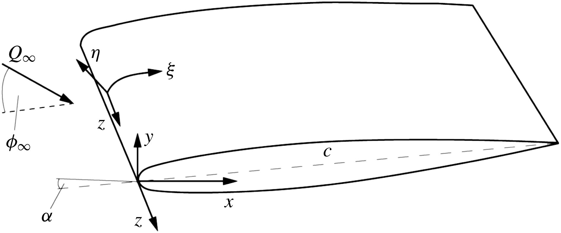
The wing geometry used in the present investigation is a swept ONERA-D airfoil with a chord length of
 $c=0.35~\text{m}$
, measured normal to the leading edge. The geometry is invariant in the spanwise direction. The flow configuration follows experiments by Kim et al. (Reference Kim, Forte and Choi2016), performed within the European project BUTERFLI in the ONERA TRIN1 wind tunnel. The model has been installed with a sweep angle of
 $\unicode[STIX]{x1D719}_{\infty }=60^{\circ }$
and at an angle of attack of
 $\unicode[STIX]{x1D6FC}=-8^{\circ }$
. The unit Reynolds number is
 $Re_{L}=Q_{\infty }L/\unicode[STIX]{x1D708}=4.4\times 10^{6}$
, with
 $L=1~\text{m}$
being the reference length scale,
 $Q_{\infty }=70~\text{m}~\text{s}^{-1}$
the total incoming free-stream velocity and
 $\unicode[STIX]{x1D708}$
the kinematic viscosity. In this work
 $Q_{\infty }$
is used to normalise velocities. The ring-type plasma actuators with spanwise spacing of
 $L_{pa}=3.5~\text{mm}$
and diameter
 $d_{pa}=1~\text{mm}$
are placed in the leading-edge region of the swept wing at the chordwise location of
 $x/c=0.019$
in the experiments. This location is too close to the attachment line,
 $x/c=0.013$
, and does not allow for the introduction of stationary and non-stationary disturbances upstream of the actuators in the numerical set-up. Therefore, the centres of the actuators are shifted to the chordwise location of
 $x/c=0.05$
, which is slightly downstream of the neutral point of the most unstable stationary cross-flow mode located around
 $x/c=0.035$
. The stationary cross-flow mode with a spanwise wavelength of 3.5 mm becomes unstable around
 $x/c=0.046$
. The boundary layer is most receptive to actuation close to the neutral point; thus shifting the location should increase the effect of actuators on the evolution of the disturbances.
Swept ONERA-D airfoil with sweep angle
 $\unicode[STIX]{x1D719}_{\infty }$
and total incoming velocity
 $Q_{\infty }$
. The Cartesian and curvilinear coordinate systems are denoted
 $(x,y,z)$
and
 $(\unicode[STIX]{x1D709},\unicode[STIX]{x1D702},z)$
, respectively, and
 $c$
denotes the chord length normal to the leading edge. The wing is under an angle of attack
 $\unicode[STIX]{x1D6FC}=-8^{\circ }$
.

Figure 1 shows the airfoil shape and the coordinate systems used in this study. The Cartesian coordinates
 $(x,y,z)$
denote the chordwise, chord-normal and spanwise directions, and the corresponding velocity components are denoted as
 $(u,v,w)$
. The body-fitted curvilinear coordinates
 $(\unicode[STIX]{x1D709},\unicode[STIX]{x1D702},z)$
define the tangential, wall-normal and spanwise directions, with the corresponding velocity components denoted as
 $(u_{\unicode[STIX]{x1D709}},v_{\unicode[STIX]{x1D702}},w)$
.
2.1 Direct numerical simulations
We consider incompressible Navier–Stokes equations subjected to constant fluid properties together with the continuity equation:
 $$\begin{eqnarray}\displaystyle \frac{\unicode[STIX]{x2202}\boldsymbol{u}}{\unicode[STIX]{x2202}t}=-\boldsymbol{u}\boldsymbol{\cdot }\unicode[STIX]{x1D735}\boldsymbol{u}-\unicode[STIX]{x1D735}p+\frac{1}{Re}\unicode[STIX]{x1D6FB}^{2}\boldsymbol{u}+\boldsymbol{f},\quad \unicode[STIX]{x1D735}\boldsymbol{\cdot }\boldsymbol{u}=0, & & \displaystyle\end{eqnarray}$$
where
 $\boldsymbol{u}=\{u,v,w\}^{\text{T}}$
is the velocity vector with components in the
 $x$
,
 $y$
and
 $z$
directions,
 $p$
represents the pressure and
 $\boldsymbol{f}$
is the body-force term. Equations (2.1) are integrated in time using the Nek5000 code developed by Fischer, Lottes & Kerkemeier (Reference Fischer, Lottes and Kerkemeier2008). Nek5000 is based on the spectral element method (SEM) proposed by Patera (Reference Patera1984), which combines the geometric flexibility of the finite element method with spectral accuracy. The physical domain in SEM is decomposed into spectral elements. Then, the local approximation of the flow field is obtained as a sum of Lagrange interpolants defined by an orthogonal basis of Legendre polynomials up to degree
 $N$
. The same polynomial order
 $N$
is used for all spatial directions. Following the
 $\mathbb{P}_{N}$
–
 $\mathbb{P}_{N-2}$
spatial discretisation (Maday & Patera Reference Maday and Patera1989),
 $N+1$
Gauss–Lobatto–Legendre (GLL) nodes are used to build the velocity Lagrange polynomial interpolants and
 $N-1$
Gauss–Legendre (GL) nodes for the pressure Lagrange polynomial interpolants (two orders less than the velocity field) in every spectral element. Here we have used
 $N=11$
for most of the simulations. The equations are advanced in time using a third-order conditionally stable backward differentiation and extrapolation scheme (BDFk/EXTk), employing an implicit treatment of the diffusion term and explicit treatment of the advection term. Nek5000 is highly parallelised and scalable on thousands of threads (Tufo & Fischer Reference Tufo and Fischer2001). The presented results are obtained using up to 4096 processors.
Several sets of simulations have been carried out in this work, in which (i) the three-dimensional laminar base flow is computed, (ii) steady cross-flow vortices are excited by means of modelled natural surface roughness, (iii) uncontrolled transition is triggered by introducing non-stationary perturbations inside the boundary layer, and (iv) the change of transition location due to the action of distributed ring-type plasma actuators is studied.
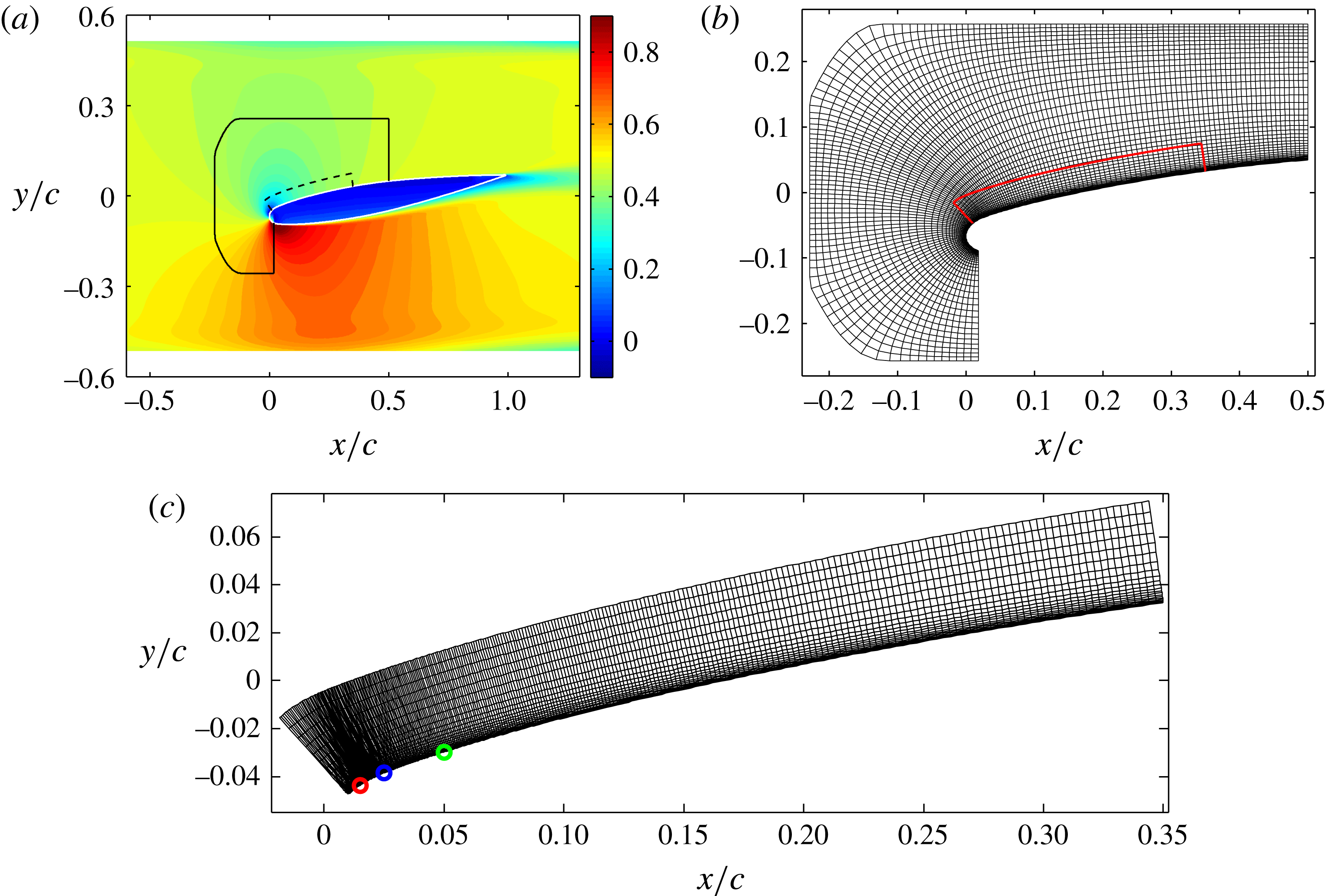
(a) Pseudo-colours of streamwise velocity component obtained from RANS solution of the entire wind tunnel test section. The black solid and dashed lines show the boundaries of the DNS domain for the laminar base-flow and receptivity computations, respectively. (b) Distribution of spectral elements for the base-flow computation and (c) distribution of the spectral elements for the receptivity computations. Red, blue and green circles depict the location of the modelled natural surface roughness, random volume force and plasma actuators, respectively.

2.2 Computational domain and boundary conditions
Prior to performing DNS computations, a complementary Reynolds-averaged Navier–Stokes (RANS) solution is obtained around the same geometry with identical flow configuration, depicted in figure 2(a). The computational domain in the RANS computation includes the top and bottom walls of the experimental test section. In spanwise direction, an infinite extension of the tunnel is assumed (corresponding to infinite swept-wing approximation). In these computations, the laminar–turbulent transition was triggered at
 $x/c=0.01$
(close to minimum pressure) on the lower side of the wing and at
 $x/c=0.8$
on the upper side by turning on the turbulence production. This has been done to avoid unsteady RANS solution due to laminar separation. The calculations have been performed with the Edge code (Eliasson Reference Eliasson2002) using Wallin & Johansson’s (Reference Wallin and Johansson2000) EARSM together with Hellsten’s (Reference Hellsten2005)
 $k$
–
 $\unicode[STIX]{x1D714}$
model. Two different numerical domains are used in the DNS computations, the boundaries of which are shown in figure 2(a). The larger domain with two outflow boundaries is used for the laminar base-flow computation. The values of velocity and pressure on the boundaries are taken from the RANS simulations described above. This is explained in detail later in the text. Although we are only interested in the flow field on the upper wing side, the base-flow domain extends to the lower wing side to account for the asymmetry of the configuration. The lower wing part and the leading-edge region are discarded in the simulations of the perturbed flow, which are performed in the smaller domain shown in figure 2(c). This is possible since the disturbances are introduced locally within the boundary layer and external sources of perturbation, such as sound waves or free-stream turbulence, are absent. The inflow and free-stream boundary conditions for the perturbed flow are of Dirichlet type and taken from the laminar base-flow solution. The outflow boundary conditions are the natural boundary conditions (
 $[1/Re(\unicode[STIX]{x1D735}\boldsymbol{u})-p\boldsymbol{I}]\boldsymbol{\cdot }\boldsymbol{n}=0$
) derived from the weak form of the Navier–Stokes equations.
The boundary conditions for the base-flow computation (larger domain with two outflow boundaries) are described in the following. Dirichlet boundary conditions are set at the inflow plane using the RANS solution
 $$\begin{eqnarray}\displaystyle \{u,v,w\}^{\text{T}}=\{u_{RANS},v_{RANS},w_{RANS}\}^{\text{T}}\quad \text{on}~\unicode[STIX]{x2202}\unicode[STIX]{x1D6FA}_{inflow}. & & \displaystyle\end{eqnarray}$$
The outflow boundary conditions are a modified version of the natural boundary conditions
 $$\begin{eqnarray}\displaystyle \frac{1}{Re}\frac{\unicode[STIX]{x2202}u}{\unicode[STIX]{x2202}x}-p=-p_{a},\quad \frac{\unicode[STIX]{x2202}v}{\unicode[STIX]{x2202}x}=0,\quad \frac{\unicode[STIX]{x2202}w}{\unicode[STIX]{x2202}x}=0\quad \text{on}~\unicode[STIX]{x2202}\unicode[STIX]{x1D6FA}_{outflow}. & & \displaystyle\end{eqnarray}$$
Here,
 $p_{a}$
stands for the prescribed pressure and
 $p_{a}=0$
results in the standard natural boundary conditions that are used in the perturbed flow simulations. It is worth mentioning that the natural conditions are not enforced explicitly but are satisfied intrinsically by the numerical solver used in this work. In boundary-layer flows, the standard natural boundary conditions force the pressure value to be zero at the junction between the outflow and the wall,
 $p_{wall}=0$
, since the streamwise derivative of the velocity vanishes at the wall (
 $\unicode[STIX]{x2202}_{x}u=0$
at the wall). Setting the pressure value to zero is not problematic since a correct pressure gradient is achievable with only one fixed pressure value in the domain. However, in flow configurations with multiple outflows, using the standard outflow boundary conditions results in fixing the pressure value to zero at multiple locations. Therefore, the pressure gradient would depend on the relative location of the outflow boundaries, which makes the results domain-dependent. This problem is avoided by prescribing a priori known pressure at the outflow boundaries, which in turn sets the correct pressure gradient in a domain with multiple outflows. In this work, the pressure field obtained from the RANS solution is used to set the pressure at the outflow boundaries for the base-flow computation,
 $p_{a}=p_{RANS}-Re^{-1}\unicode[STIX]{x2202}_{x}u_{RANS}$
.
The free-stream boundary conditions are of Dirichlet type in the streamwise and spanwise directions along with the modified natural condition normal to the boundary surface
 $$\begin{eqnarray}\displaystyle u=u_{RANS},\quad \frac{1}{Re}\frac{\unicode[STIX]{x2202}v}{\unicode[STIX]{x2202}y}-p=p_{a},\quad w=w_{RANS}\quad \text{on}~\unicode[STIX]{x2202}\unicode[STIX]{x1D6FA}_{freestream}. & & \displaystyle\end{eqnarray}$$
The prescribed pressure at the free stream is set to
 $p_{a}=p_{RANS}-Re^{-1}\unicode[STIX]{x2202}_{y}v_{RANS}$
to account for the non-zero pressure gradient around the wing.
In all the simulations except the base-flow computation, sponge regions are inserted in the vicinity of the outflow boundaries to avoid numerical instabilities. Within the sponge region, the flow is forced towards the laminar base flow. This is achieved by adding the forcing term
 $$\begin{eqnarray}\displaystyle \boldsymbol{F}(\boldsymbol{x},t)=A_{f}\unicode[STIX]{x1D706}_{f}(\boldsymbol{x})[\boldsymbol{U}_{f}(\boldsymbol{x})-\boldsymbol{u}(\boldsymbol{x},t)] & & \displaystyle\end{eqnarray}$$
on the right-hand side of the momentum equation. The field
 $\boldsymbol{u}=(u,v,w)^{\text{T}}$
stands for the instantaneous velocity field and
 $\boldsymbol{U}_{f}$
denotes the target solution (the laminar base flow). The function
 $\unicode[STIX]{x1D706}_{f}$
takes the form of a smooth step function, which varies between zero and one in the sponge region and vanishes elsewhere,
 $$\begin{eqnarray}\displaystyle & \displaystyle \unicode[STIX]{x1D706}_{f}(x)=S\left(\frac{x-x_{start}}{\unicode[STIX]{x1D6E5}_{rise}}\right), & \displaystyle\end{eqnarray}$$
 $$\begin{eqnarray}\displaystyle & \displaystyle S(\unicode[STIX]{x1D709})=\left\{\begin{array}{@{}ll@{}}0,\qquad & \unicode[STIX]{x1D709}\leqslant 0,\\ \displaystyle \left[1+\exp \left(\frac{1}{\unicode[STIX]{x1D709}-1}+\frac{1}{\unicode[STIX]{x1D709}}\right)\right]^{-1},\qquad & 0<\unicode[STIX]{x1D709}<1,\\ 1,\qquad & \unicode[STIX]{x1D709}\geqslant 1.\end{array}\right. & \displaystyle\end{eqnarray}$$
Here,
 $\unicode[STIX]{x1D6E5}_{rise}=0.005$
and
 $x_{start}$
are chosen such that the sponge length in the streamwise direction is 5 % of the chord length. The coefficient
 $A_{f}$
determines the maximal strength of the forcing and is set to
 $A_{f}=100$
in this study. This value and the length of the sponge region have been chosen empirically such that the perturbations vanish at the end of the sponge region and the outflow conditions behave correctly, not introducing any numerical noise.
The distributions of the spectral elements in the computational domains used in the base-flow and receptivity simulations are shown in figure 2(b,c), respectively. The mesh has been generated using the gridgen-c code by Sakov (Reference Sakov2011), which provides quasi-orthogonal grids. The base-flow domain extends from
 $x/c=0.018$
on the lower side of the wing to
 $x/c=0.5$
on the upper wing side. The domain for receptivity computations extends over
 $x/c=0.01{-}0.35$
on the upper wing side. The two-dimensional mesh for the base-flow and receptivity computations consists of 6300 and 6210 spectral elements, respectively. The minimum and maximum grid spacings along the surface in the base-flow mesh are
 $\min (\unicode[STIX]{x0394}S/c)=2.0\times 10^{-4}$
and
 $\max (\unicode[STIX]{x0394}S/c)=1.0\times 10^{-3}$
, and in the wall-normal direction
 $\min (\unicode[STIX]{x0394}y/c)=2.4\times 10^{-6}$
and
 $\max (\unicode[STIX]{x0394}y/c)=1.5\times 10^{-3}$
. The corresponding values for the receptivity mesh are
 $\min (\unicode[STIX]{x0394}S/c)=6.9\times 10^{-6}$
and
 $\max (\unicode[STIX]{x0394}S/c)=3.9\times 10^{-4}$
, and
 $\min (\unicode[STIX]{x0394}y/c)=1.1\times 10^{-6}$
and
 $\max (\unicode[STIX]{x0394}y/c)=6.2\times 10^{-4}$
.
In the experimental study by Kim et al. (Reference Kim, Forte and Choi2016), a spanwise array of ring-type plasma actuators is inserted near the leading edge of the swept wing as a control mechanism to delay transition. The spacing between the actuators is
 $L_{pa}=3.5~\text{mm}$
, which corresponds to approximately two-thirds of the wavelength of the naturally most unstable stationary cross-flow mode (Saric et al.
Reference Saric, Ruben and Reibert1998; Hosseini et al.
Reference Hosseini, Tempelmann, Hanifi and Henningson2013). In order to simultaneously excite the most unstable stationary mode and the control mode (induced by the wall-normal jet of the plasma actuators), a spanwise length of
 $L_{z}=3\times 3.5=10.5~\text{mm}$
is considered, which dictates a fundamental spanwise wavenumber
 $\unicode[STIX]{x1D6FD}_{0}=2\unicode[STIX]{x03C0}/L_{z}=598~\text{rad}~\text{m}^{-1}$
. We mimic the actuator row by prescribing spanwise periodic boundary conditions. The two-dimensional mesh presented in figure 2(c) is extended in the spanwise direction. In the spanwise direction 36 spectral elements are uniformly distributed to resolve a span of length
 $L_{z}$
. The total number of three-dimensional spectral elements amounts to 223 560, and using a polynomial order of
 $N=11$
for the velocities results in
 ${\approx}386\times 10^{6}$
grid points.
2.3 Stationary perturbations
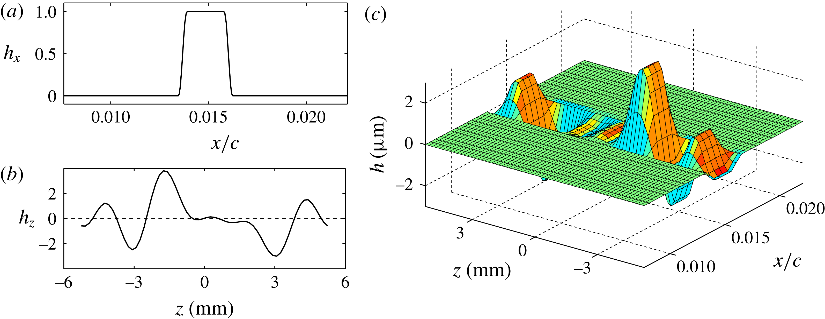
In the experimental studies, stationary cross-flow vortices, including the naturally most unstable ones, are excited due to the presence of the natural surface roughness in the leading-edge region of the wing. In this work, the natural surface roughness, which is localised along the chord and periodic in the spanwise direction, is modelled by
 $$\begin{eqnarray}\displaystyle h(x,z)=\unicode[STIX]{x1D700}_{h}h_{x}(x)h_{z}(z), & & \displaystyle\end{eqnarray}$$
where
 $\unicode[STIX]{x1D700}_{h}$
is the maximum amplitude of the roughness bump and
 $h_{x}(x)$
and
 $h_{z}(z)$
are shape functions in the streamwise and spanwise directions. The shape function
 $h_{x}(x)$
is described by
 $$\begin{eqnarray}\displaystyle h_{x}(x)=S\left(\frac{x-h_{s}}{h_{r}}\right)-S\left(\frac{x-h_{e}}{h_{f}}+1\right), & & \displaystyle\end{eqnarray}$$
where
 $S$
is the smooth step function defined in (2.7). The roughness bump in the streamwise direction starts at
 $x=h_{s}$
, rises smoothly along the distance
 $h_{r}$
and ends at
 $x=h_{e}$
with a falling distance of
 $h_{f}$
. The centre of the roughness is located at
 $x_{r}=(h_{s}+h_{e})/2$
. This shape of roughness contains a broad spectrum of streamwise wavenumbers, including the unstable ones. In this study, the natural surface roughness is centred at
 $x/c=0.015$
with a total width of 1 mm. The rise and fall distances are equal and set to
 $h_{r}=h_{f}=0.2~\text{mm}$
. The spanwise periodic shape function
 $h_{z}(z)$
is defined as
 $$\begin{eqnarray}\displaystyle h_{z}(z)=\mathop{\sum }_{n=1}^{5}\sin (n\unicode[STIX]{x1D6FD}_{0}z+\unicode[STIX]{x1D719}_{n}^{rand}), & & \displaystyle\end{eqnarray}$$
where
 $\unicode[STIX]{x1D719}_{n}^{rand}=[2.8,2.4,4.8,5.0,1.2]$
are random phases and
 $\unicode[STIX]{x1D6FD}_{0}=2\unicode[STIX]{x03C0}/L_{z}$
with
 $L_{z}=10.5~\text{mm}$
.
The natural surface roughness is not meshed but modelled by inhomogeneous boundary conditions at the wall. The no-slip conditions along the roughness
 $h(x,z)$
are projected from the bump surface to the wall via a Taylor series expansion,
 $$\begin{eqnarray}\displaystyle \{u,v,w\}_{wall}^{\text{T}}=\left\{-h(x,z)\frac{\unicode[STIX]{x2202}U}{\unicode[STIX]{x2202}y},~0,~-h(x,z)\frac{\unicode[STIX]{x2202}W}{\unicode[STIX]{x2202}y}\right\}_{wall}^{\text{T}},\quad h_{s}\leqslant x\leqslant h_{e}, & & \displaystyle\end{eqnarray}$$
where
 $U$
and
 $W$
are the laminar base-flow velocities. Since the roughness height
 $\unicode[STIX]{x1D700}_{h}$
is assumed to be small, the Taylor series is truncated at the first order. The roughness height
 $\unicode[STIX]{x1D700}_{h}$
is chosen such that the root-mean-square (r.m.s.) value of
 $h(x,z)$
at the roughness centre matches the reported r.m.s. roughness height of
 $1~\unicode[STIX]{x03BC}\text{m}$
in the experiment.
Distributions of the shape function (a)
 $h_{x}$
in the streamwise direction and (b)
 $h_{z}$
in the spanwise direction, plotted at
 $x/c=0.015$
; and (c) visualisation of the natural surface roughness.

2.4 Non-stationary perturbations
Generation of the unsteady instability waves, both primary and secondary, requires the presence of unsteady disturbances such as acoustic noise or free-stream turbulence. In this study, non-stationary perturbations are artificially induced inside the boundary layer by employing a weak randomly pulsed volume force. The forcing acts only in the wall-normal direction and is intended to introduce unsteady perturbations within a specific range of wavenumber and frequency.
The forcing enters the wall-normal momentum equation as
 $$\begin{eqnarray}\displaystyle F_{y}=\exp \{-[(x-x_{0})/l_{x}]^{2}-[(y-y_{0})/l_{y}]^{2}\}g(z,t), & & \displaystyle\end{eqnarray}$$
where the forcing
 $g(z,t)$
varies in time and spanwise direction, and it is mapped into a Gaussian shape with
 $l_{x}$
and
 $l_{y}$
being the Gaussian attenuation of the forcing region. The location of the force is centred at the coordinates
 $x_{0}$
and
 $y_{0}$
. The distribution of
 $g(z,t)$
in time and space reads
 $$\begin{eqnarray}\displaystyle g(z,t)=A_{t}[(1-b(t))h^{i}(z)+b(t)h^{i+1}(z)], & & \displaystyle\end{eqnarray}$$
with
 $b(t)=3p^{2}-2p^{3}$
,
 $p=t/t_{s}-i$
and
 $i=\text{int}(t/t_{s})$
where
 $\text{int}(\cdot )$
represents the integer part of the argument. The temporal scale is represented by
 $t_{s}$
, which is in effect the cut-off frequency of the perturbations. A third-order Lagrangian interpolation is used in order to interpolate
 $g(z,t)$
in time. The values of
 $h^{i}(z)$
are random harmonic functions having a unit amplitude for wavenumbers below
 $2\unicode[STIX]{x03C0}/z_{s}$
and zero amplitude for wavenumbers above that range. A pseudo-random number generator, which enables accurate restart of the simulations, was used to generate the spanwise distribution.
The forcing is located downstream of the natural surface roughness at
 $x_{0}/c=0.024$
and
 $y_{0}/c=0.039$
and its shape is attenuated by a Gaussian in the streamwise and wall-normal directions employing parameters
 $l_{x}=l_{y}=2\times 10^{-3}$
. We have placed the volume force just downstream of the surface roughness in order to introduce the unsteady perturbations into the set-up as soon as possible. The temporal cut-off scale corresponds to a frequency of
 ${\approx}7000~\text{Hz}$
and the spanwise cut-off wavenumber corresponds to
 $30\unicode[STIX]{x1D6FD}_{0}$
. The amplitude of the forcing is chosen such that the transition is obtained at
 ${\sim}20\,\%$
chord, similar to the transition location observed in the experiments
 $(A_{t}=0.01)$
. For more details and insight about this method, the reader is referred to Örlü & Schlatter (Reference Örlü and Schlatter2013) and Hosseini et al. (Reference Hosseini, Vinuesa, Schlatter, Hanifi and Henningson2016).
2.5 Plasma actuator body-force field
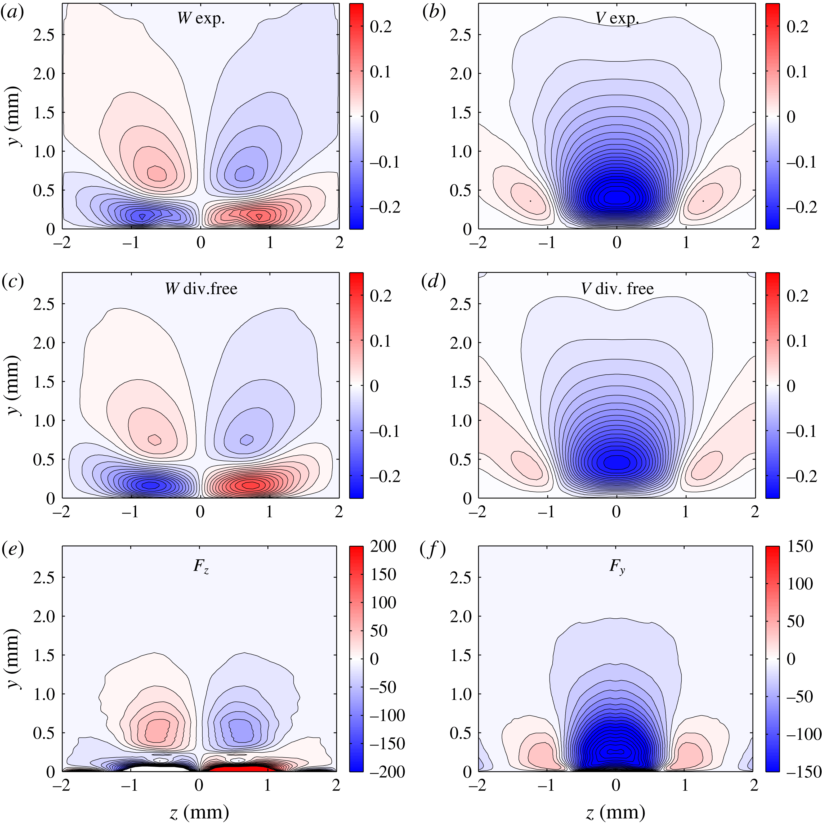
The ring-type DBD plasma actuator produces a wall-normal jet in the experiments, which acts as a virtual roughness element. The action of the actuators in the numerical simulations is incorporated by a body force that corresponds to the velocity field produced by an actuator in quiescent air. Such a velocity field is provided by Kim & Choi (Reference Kim and Choi2016), who placed an actuator sheet on a flat plate and measured the velocity field induced by the actuators in quiescent air. The actuators were active under 5.8 kV power supply and at 40 kHz frequency. The measured velocity field is averaged in time and space, which results in a steady body force in the numerical simulations. For a ring-type plasma actuator, the induced velocity field is symmetric in the radial direction around the centre of the actuator. Figure 4(a,b) shows the experimental spanwise and wall-normal velocity fields induced by a spanwise periodic array of ring-type plasma actuators. As can be seen there, the air is pushed upwards around the actuator and downwards in the centre of it. This creates jet flows when actuators are placed periodically in a row. In this section, velocity and body force are presented in dimensional values.
(a,b) Experimental spanwise and wall-normal velocity components, (c,d) divergence-free spanwise and wall-normal velocity components, and (e,f) the corresponding steady force field in the spanwise and wall-normal directions. All the planes are at
 $x=0$
. Some 32 equi-spaced contours in the range
 $[-0.25,0.25]$
and
 $[-0.3,0.1]$
are shown for the spanwise and wall-normal velocity components, respectively.

Nek5000 is used to calculate the body force from the experimentally measured velocity field induced by a ring-type plasma actuator in quiescent air. The steady body force can be obtained by evaluating
 $$\begin{eqnarray}\displaystyle -\boldsymbol{f}=-\boldsymbol{u}\boldsymbol{\cdot }\unicode[STIX]{x1D735}\boldsymbol{u}-\unicode[STIX]{x1D735}p+\frac{1}{Re}\unicode[STIX]{x1D6FB}^{2}\boldsymbol{u}, & & \displaystyle\end{eqnarray}$$
where
 $\boldsymbol{u}$
and
 $p$
are the experimental velocity and pressure fields. Instead of evaluating the individual terms on the right-hand side of (2.14), the whole sum can be evaluated by computing the first-order time derivative using the numerical solver,
 $$\begin{eqnarray}\displaystyle \frac{\boldsymbol{u}^{(1)}-\boldsymbol{u}^{(0)}}{\unicode[STIX]{x0394}t}=-\boldsymbol{u}\boldsymbol{\cdot }\unicode[STIX]{x1D735}\boldsymbol{u}-\unicode[STIX]{x1D735}p+\frac{1}{Re}\unicode[STIX]{x1D6FB}^{2}\boldsymbol{u}. & & \displaystyle\end{eqnarray}$$
Here
 $\boldsymbol{u}^{(0)}$
and
 $\boldsymbol{u}^{(1)}$
are the velocity vectors at the zeroth and first time step, respectively. This procedure can be interpreted physically as balancing unsteadiness in the flow (in the absence of body force) with a force field; thus the flow with such a force field becomes steady. Using this method has two main advantages. First, the original velocity field is made divergence-free with Nek5000 to any desired numerical tolerance. Secondly, the pressure-gradient term can be kept in the calculation of the force field, which is commonly neglected in other methods of computing the body force based on velocity information (for pressure-gradient effect on the body force see Dörr & Kloker (Reference Dörr and Kloker2015a
)).
The experimental velocity field is interpolated on a three-dimensional Cartesian domain with the centre of the plasma actuator positioned at the origin. Homogeneous Dirichlet boundary conditions are applied on all the far-field boundaries of the domain in the streamwise and wall-normal directions. Periodic boundary conditions are applied in the spanwise direction. The time integration scheme is set to first order with a time step
 $\unicode[STIX]{x0394}t=10^{-4}$
. The solver tolerance for both velocity and pressure solvers is chosen to be
 $10^{-8}$
and the polynomial order is set to
 $N=8$
.
Figure 4(a,b) shows the experimental spanwise and wall-normal velocity components in the wall-normal spanwise plane at
 $x=0$
. The divergence-free velocity fields
 $\boldsymbol{u}^{(0)}$
are shown in figure 4(c,d) and the computed body force based on the evaluation of (2.15) is demonstrated in figure 4(e,f).
Steady-state DNS velocity fields induced by the plasma actuator body force in quiescent air. (a) The spanwise and (b) the wall-normal velocity component. All the planes are at
 $x=0$
. The contour levels are the same as in figure 4.

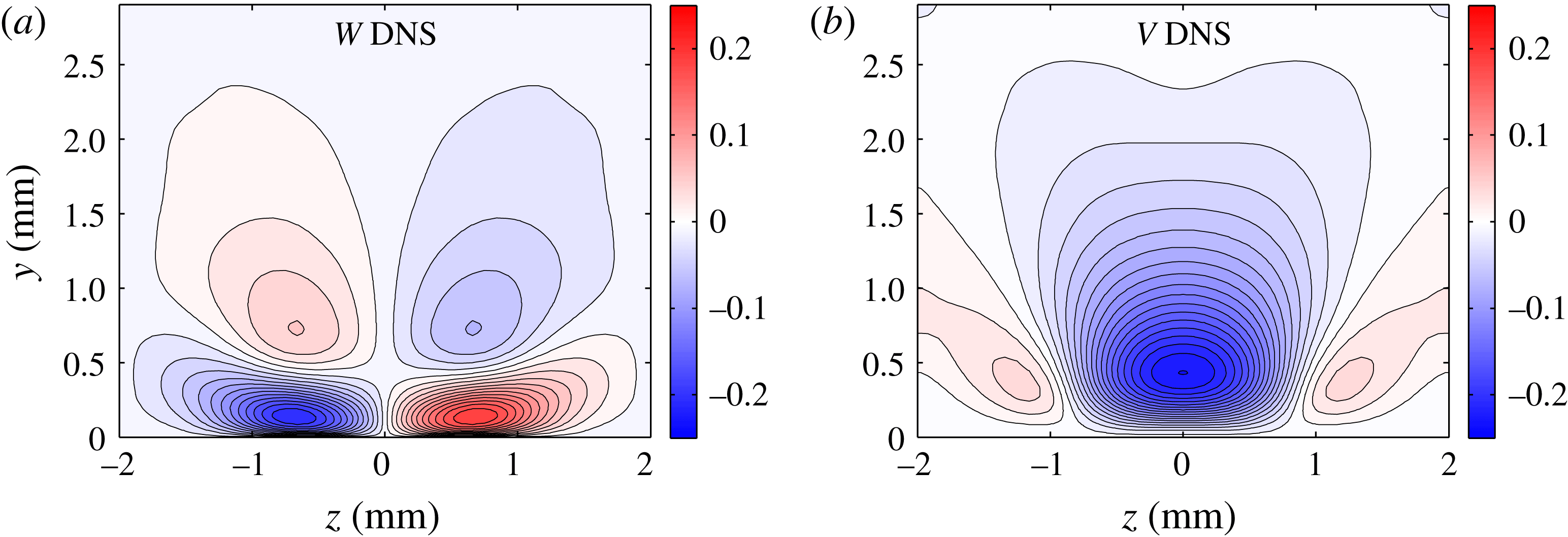
The computed force field is validated by performing a simulation in quiescent air and comparing the velocity field induced by the body force with the original velocity field. For this purpose the boundary condition at the most downstream streamwise plane is changed to outflow condition (instead of the homogeneous Dirichlet condition used in computation of the force term). The reason behind this is basically to avoid possible numerical instabilities at the beginning of the simulation. The boundary condition at the inflow plane and at the far field in the wall-normal direction is kept as homogeneous Dirichlet conditions. Figure 5 shows the steady-state solution resulting from the plasma actuator body force in quiescent air. Comparison of figure 5 and the divergence-free original velocity field in figure 4(c,d) demonstrates that the computed plasma actuator force field in the numerical simulations generates the corresponding velocity field produced by the plasma actuators in the experiments.
In reality, the airflow influences the performance of a plasma actuator. But, for the airflow speed of the current experiment, the reduction in efficiency of the actuator is expected to be less than 10 % (see Kriegseis, Grundmann & Tropea Reference Kriegseis, Grundmann and Tropea2012). Therefore, in the present work we simply use the force field obtained for the quiescent condition.
3 Results
3.1 Laminar base flow
Since base flow is homogeneous in the spanwise direction (
 $\unicode[STIX]{x2202}_{z}p=0$
), the spanwise momentum equation is decoupled from the other two momentum equations and acts as a passive scalar transport. Therefore, laminar base flow is computed, at a significantly lower numerical cost, via a two-dimensional simulation in which the spanwise velocity component is computed as a passive scalar,
 $$\begin{eqnarray}\displaystyle \unicode[STIX]{x1D70C}c_{p}\frac{\unicode[STIX]{x2202}W}{\unicode[STIX]{x2202}t}=-(\boldsymbol{u}\boldsymbol{\cdot }\unicode[STIX]{x1D735})W+\unicode[STIX]{x1D705}\unicode[STIX]{x1D6FB}^{2}W, & & \displaystyle\end{eqnarray}$$
where the thermal conductivity is set to
 $\unicode[STIX]{x1D705}=Re^{-1}$
and
 $\unicode[STIX]{x1D70C}c_{p}=1$
.
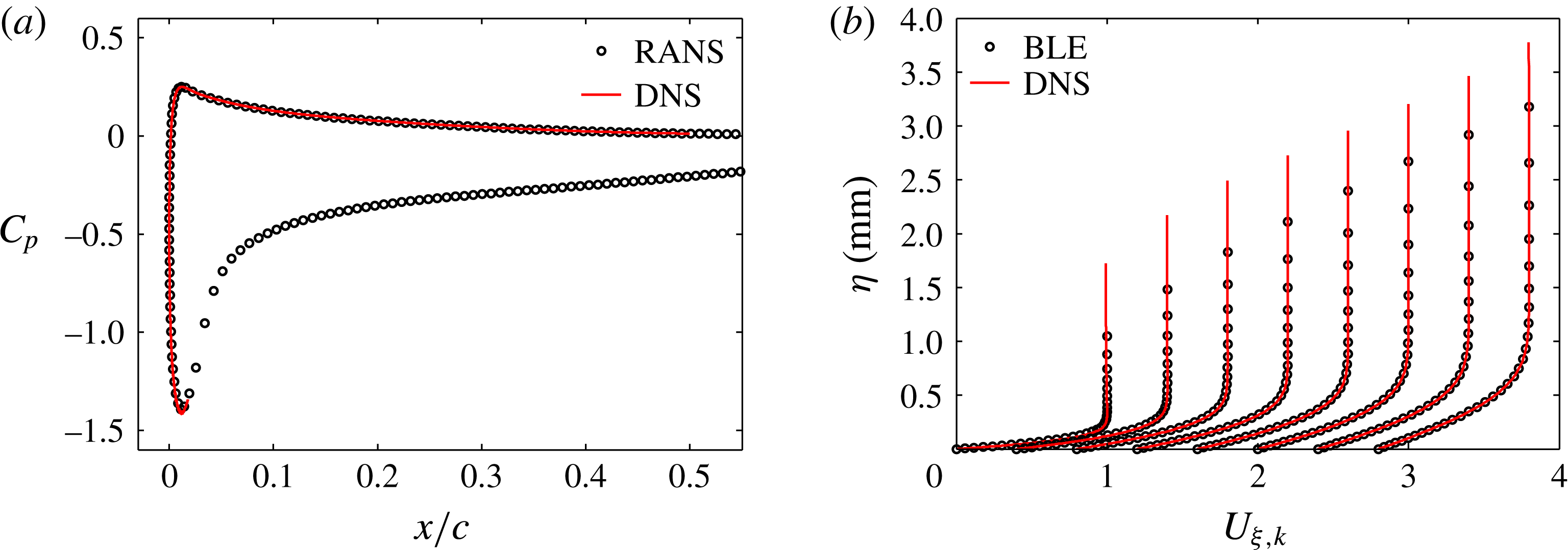
(a) Distribution of the pressure coefficient
 $C_{p}$
obtained from the DNS and the RANS solutions. (b) Boundary-layer profiles of the tangential velocity obtained from the DNS and the BLE solutions. For clarity, the profiles are shifted according to
 $U_{\unicode[STIX]{x1D709},k}=U_{\unicode[STIX]{x1D709}}+0.2k$
with
 $k=0,2,4,\ldots$
changing from left to right. The profiles are evaluated at
 $x/c=0.03,0.07,0.12,0.17,0.23,0.30,0.37,0.45$
.

The pressure coefficients,
 $C_{p}$
, computed from the DNS and the RANS solutions are compared in figure 6(a). There is a close match on both the upper and the lower wing sides. This validates the modified outflow boundary conditions presented in § 2.2 and demonstrates domain-independent solutions.
Further validation of the base flow is performed by solving the quasi-three-dimensional, fully non-similar boundary-layer equations (BLEs), where the flow conditions required at the boundary-layer edge are retrieved from the pressure coefficient of the DNS solution. The equations are solved by employing second-order finite differences in both the
 $\unicode[STIX]{x1D709}$
and the
 $\unicode[STIX]{x1D702}$
directions starting from the stagnation point. The boundary-layer profiles of the tangential velocity obtained from the DNS and BLEs are compared in figure 6(b). The velocity profiles of the DNS are normalised by the maximum value in the boundary layer. The present results confirm the validity of the numerical set-up for DNS computations.
Values of
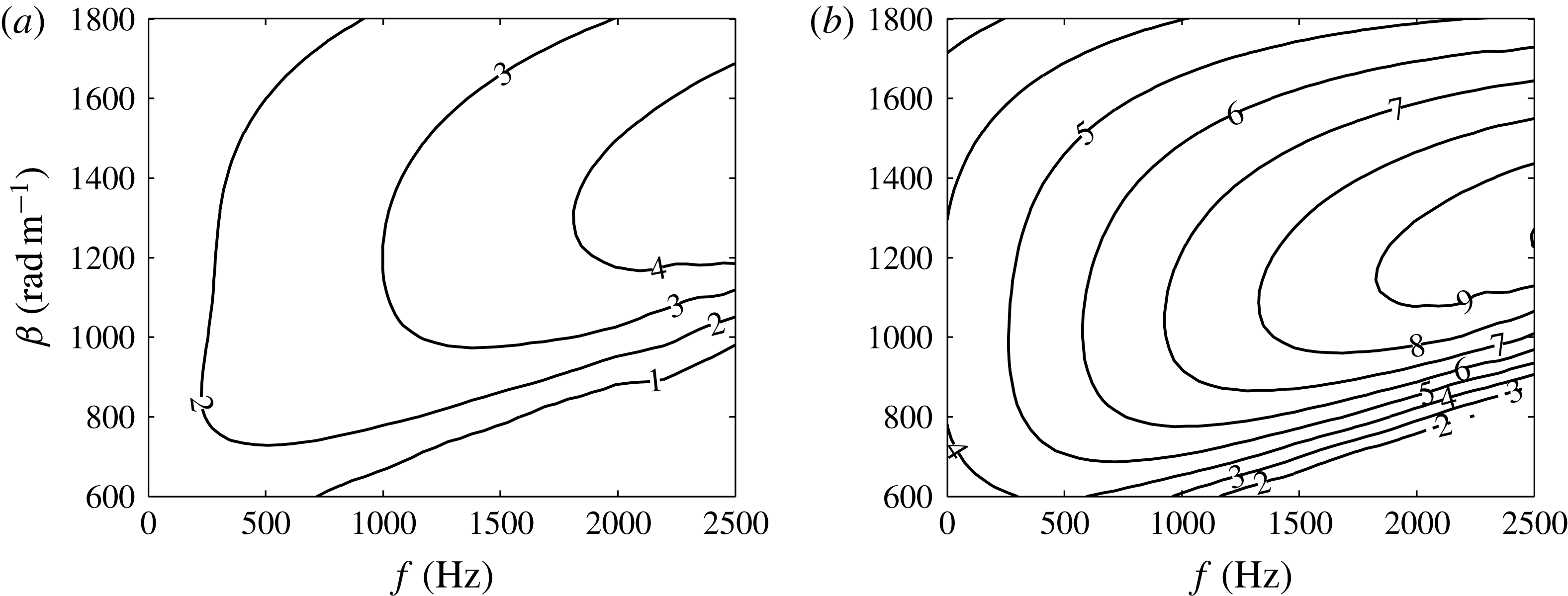
 $N$
-factor for different frequencies and spanwise wavenumbers obtained through linear PSE analysis of the underlying base flow: (a) at
 $x/c=0.1$
and (b) at
 $x/c=0.2$
.

In figure 7 the stability characteristics of the boundary layer under consideration are presented in terms of linear
 $N$
-factor values for different frequencies and spanwise wavenumbers. The stability analysis is performed in framework of the non-local/PSE theory.
3.2 Effect of control on stationary disturbances
In this section we investigate the control capability of the ring-type plasma actuator by studying its effect on the primary stationary cross-flow disturbances. To this end, two set-ups are considered. In the first set-up, stationary cross-flow vortices are excited by means of natural surface roughness only; and in the second case, the plasma actuator body force is activated in the presence of natural surface roughness. In the following these two cases are referred to as the ‘uncontrolled’ and the ‘controlled’ case, respectively.
In order to compare the uncontrolled and controlled cases quantitatively, the amplitude of individual cross-flow modes is obtained by means of Fourier transformation in the spanwise direction, i.e.
 $$\begin{eqnarray}\displaystyle u_{\unicode[STIX]{x1D709}}(\unicode[STIX]{x1D709},\unicode[STIX]{x1D702},z)=\mathop{\sum }_{n=0}^{N}\hat{u} _{\unicode[STIX]{x1D709}}(\unicode[STIX]{x1D709},\unicode[STIX]{x1D702},n\unicode[STIX]{x1D6FD}_{0})\text{e}^{\text{i}n\unicode[STIX]{x1D6FD}_{0}z}. & & \displaystyle\end{eqnarray}$$
Here,
 $\unicode[STIX]{x1D6FD}_{0}=2\unicode[STIX]{x03C0}/L_{z}$
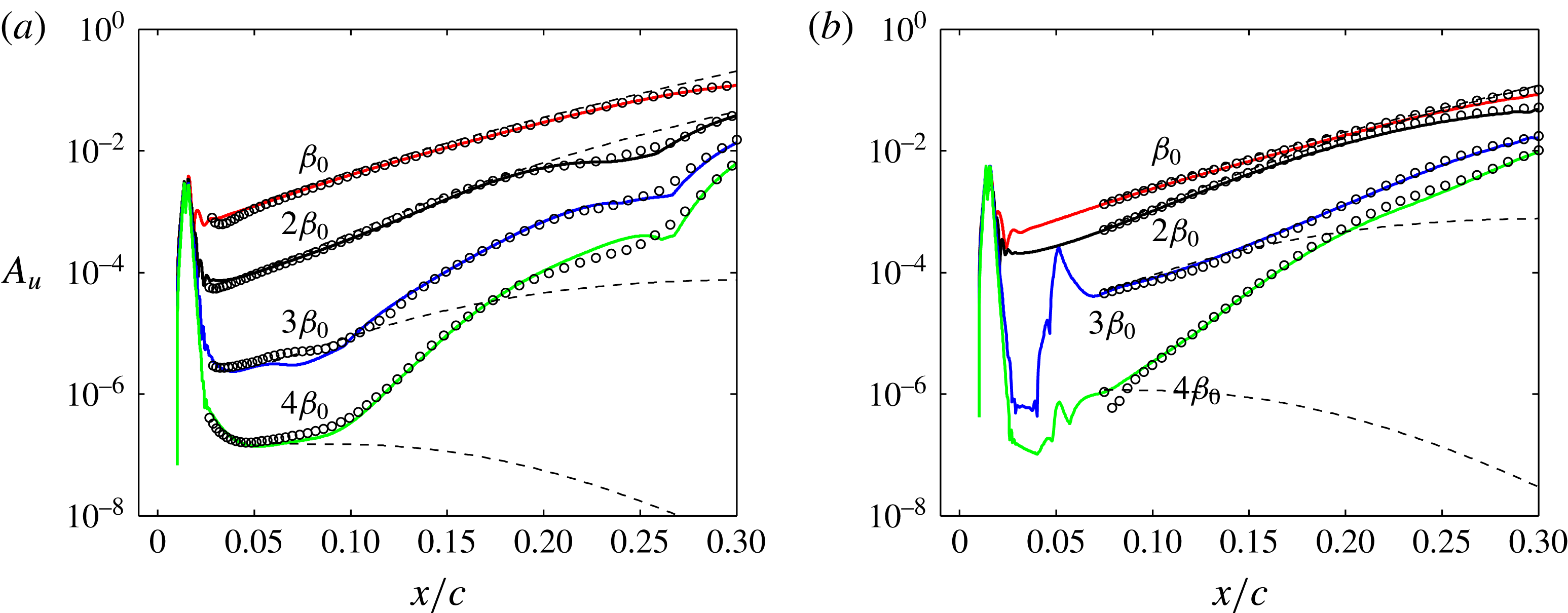
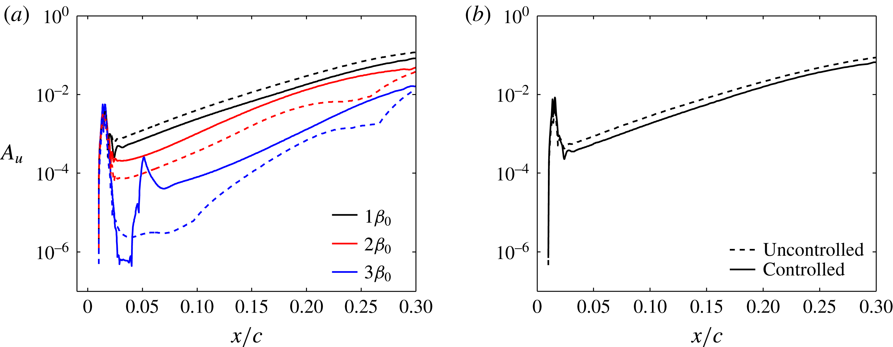
is the fundamental spanwise wavenumber dictated by the spanwise length of the domain. The amplitudes of individual modes for both the uncontrolled and controlled cases are plotted in figure 8 as
 $$\begin{eqnarray}\displaystyle A_{u}(x)=\max _{\unicode[STIX]{x1D702}}\frac{|\hat{u} _{\unicode[STIX]{x1D709}}|}{Q_{\infty }}, & & \displaystyle\end{eqnarray}$$
where
 $\hat{u} _{\unicode[STIX]{x1D709}}$
is the Fourier amplitude of the tangential velocity and
 $Q_{\infty }$
denotes the total free-stream velocity. Linear stability analysis of the underlying base flow predicts that the most unstable stationary cross-flow mode is the
 $2\unicode[STIX]{x1D6FD}_{0}$
mode. However, for both cases, the amplitude of the fundamental
 $\unicode[STIX]{x1D6FD}_{0}$
mode dominates the amplitude of its superharmonics. Although all the modes excited by natural surface roughness have identical amplitudes at the roughness location, the fundamental mode is the most receptive to the surface roughness. This is due to the fact that the neutral point of stationary modes is located around
 $x/c\approx 0.04$
and the surface roughness is positioned upstream of this location at
 $x/c=0.015$
. Therefore, modes excited by the surface roughness first decay in amplitude, with different decay rates, until they reach their corresponding neutral point and then grow and evolve moving downstream. The growth rate (slope of the amplitude curve) of the
 $2\unicode[STIX]{x1D6FD}_{0}$
mode is however larger than the fundamental mode, confirming the linear stability prediction.
Amplitude evolution
 $A_{u}$
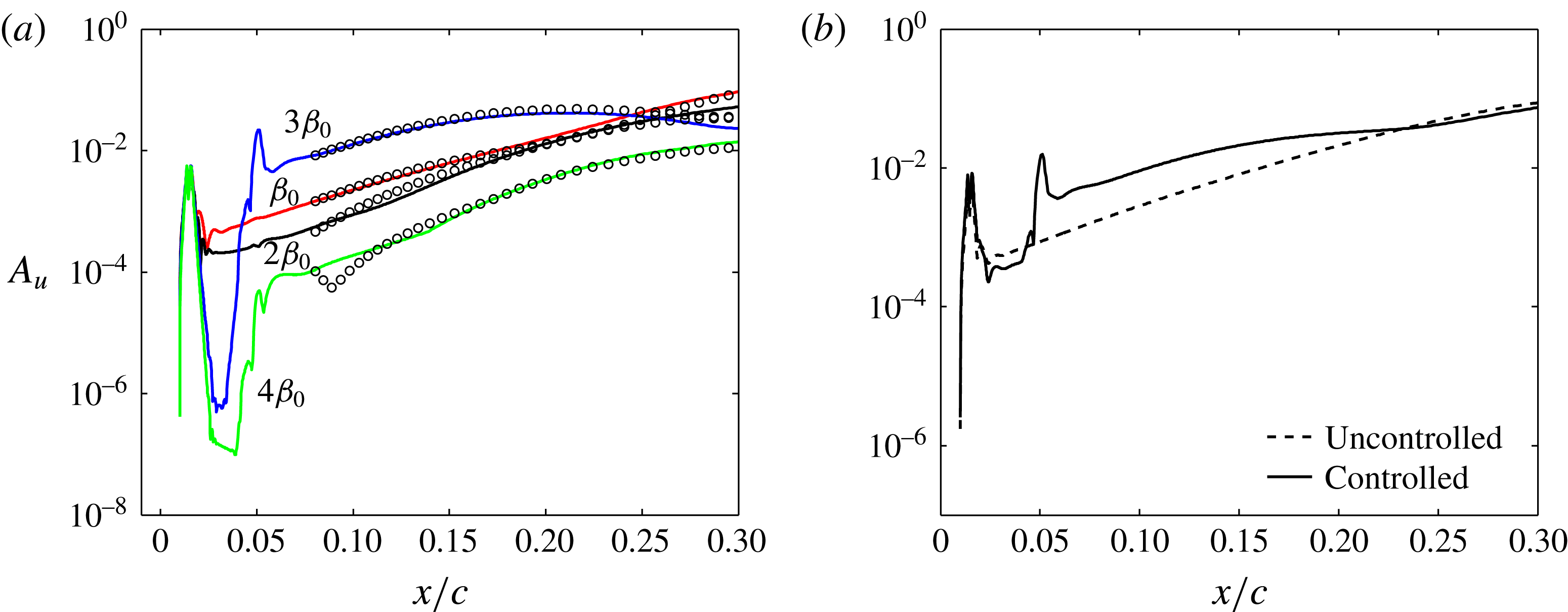
of the stationary modes for (a) uncontrolled case and (b) controlled case in the absence of unsteady perturbations. Solid lines represent DNS amplitudes; dashed lines and circular symbols show the amplitude evolution predicted by linear and nonlinear PSE, respectively.

Figure 8 also shows the amplitude evolution of different modes obtained by linear and nonlinear PSE computations on the underlying base flow. The initial amplitude of modes for nonlinear PSE computations are extracted from DNS solutions at
 $x/c=0.03$
and
 $x/c=0.075$
for the uncontrolled and controlled cases, respectively. Despite slight discrepancies between nonlinear PSE and DNS, the overall agreement is found to be very good. For both uncontrolled and controlled cases, the
 $\unicode[STIX]{x1D6FD}_{0}$
mode shows linear growth up to
 $x/c\approx 0.25$
and the
 $2\unicode[STIX]{x1D6FD}_{0}$
mode behaves linearly up to the chord length
 $x/c\approx 0.20$
. No nonlinear amplitude saturation is observed through the computational domain.
(a) Amplitude evolution of the stationary modes for both uncontrolled (dashed) and controlled (solid) cases in the absence of unsteady perturbations. (b) Amplitude (spanwise r.m.s.) of the total disturbances.

Figure 9(a) compares the amplitude evolution of the first three modes for both cases. The excitation of the
 $3\unicode[STIX]{x1D6FD}_{0}$
mode by plasma actuators in the controlled case is apparent. Subsequently, the
 $\unicode[STIX]{x1D6FD}_{0}$
mode is attenuated but the amplitude of the
 $2\unicode[STIX]{x1D6FD}_{0}$
mode is increased compared to the uncontrolled case. In order to obtain the overall effect of the control on the stationary disturbances, we extract the total amplitude of the stationary disturbances by computing the wall-normal maximum of the spanwise r.m.s. amplitude of the disturbances. The disturbance field itself is obtained by subtracting the spanwise mean velocity from the total velocity field. Figure 9(b) shows how the amplitude of total disturbances evolves in both the uncontrolled and controlled cases. It is apparent that the excitation of the control mode slightly decreases the total amplitude of the stationary disturbances. However, there is no visible local effect on the total disturbance amplitude around the location of the plasma actuator.
3.3 Unsteady disturbances and secondary instabilities
In the previous section we showed the effects of the control on the evolution of the primary stationary cross-flow disturbances when the unsteady perturbations were absent. Owing to the high accuracy of the DNS code, there was no background noise in the simulations; thus the flow did not transition to turbulence. In this section, a more realistic set-up is considered. Unsteady perturbations are introduced in the boundary layer by means of the random volume force described in § 2.4. The amplitude of the random force is chosen such that the transition occurs close to the experimental transition location. Similar to the previous section, we study an uncontrolled and a controlled case. In the former set-up, steady cross-flow disturbances are excited by the surface roughness model, while unsteady disturbances are introduced by employing the random volume force. In the controlled case, the body force modelling the plasma actuator is added to the uncontrolled set-up in order to excite the steady control mode.
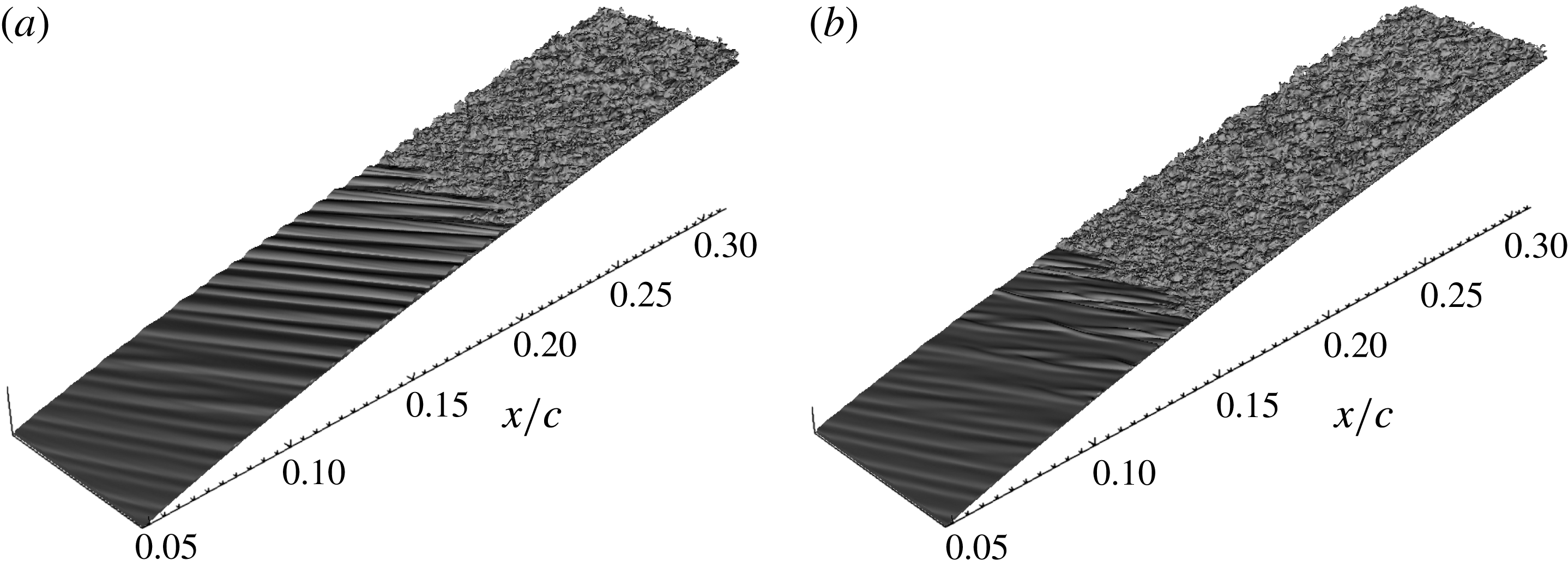
Isosurfaces of instantaneous spanwise velocity field in the (a) uncontrolled and (b) controlled cases. For better visualisation, the domain is duplicated in the spanwise direction.

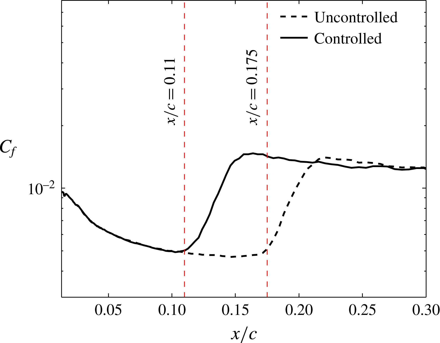
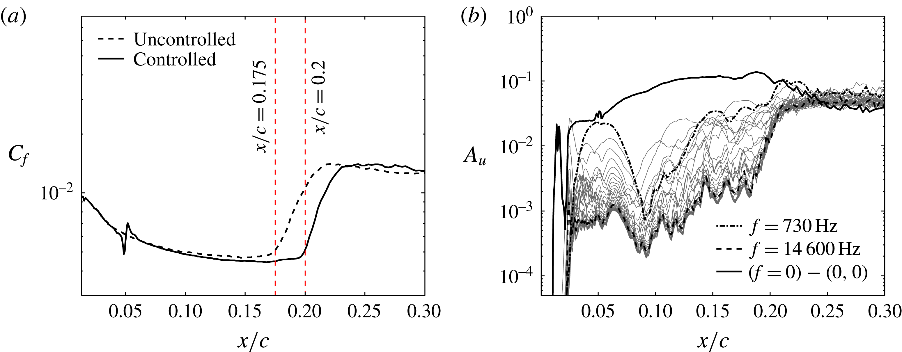
Time-averaged friction coefficient for the uncontrolled and controlled cases.

Figure 10 shows isosurfaces of instantaneous spanwise velocity for both the uncontrolled and controlled cases. Similar to the experimental observations, it is apparent that employing the control by plasma actuators has promoted transition. A quantitative measure for transition location is obtained by evaluating the wall-friction coefficient. A breakdown to turbulent flow is accompanied by a strong increase in this coefficient. Figure 11 shows time-averaged friction coefficient
 $C_{f}=2\unicode[STIX]{x1D707}(\unicode[STIX]{x2202}u_{s}/\unicode[STIX]{x2202}\unicode[STIX]{x1D702})$
for both the uncontrolled and controlled cases, where
 $u_{s}=u_{\unicode[STIX]{x1D709}}\cos (\unicode[STIX]{x1D719}_{\infty })+w\sin (\unicode[STIX]{x1D719}_{\infty })$
is the velocity in the direction of the incoming free stream. Since the perturbation field includes also unsteady cross-flow vortices, the transition location moves slightly up and down for both cases (
 $\pm 3\,\%$
chord length). Therefore, we present the time-averaged values of
 $C_{f}$
. In the uncontrolled case, transition starts at
 $x/c\approx 0.175$
with the appearance of turbulent spots and the flow becomes fully turbulent at
 $x/c\approx 0.22$
. In the controlled case, the transition location moves upstream to
 $x/c\approx 0.11$
, with a fully turbulent flow at
 $x/c\approx 0.16$
.
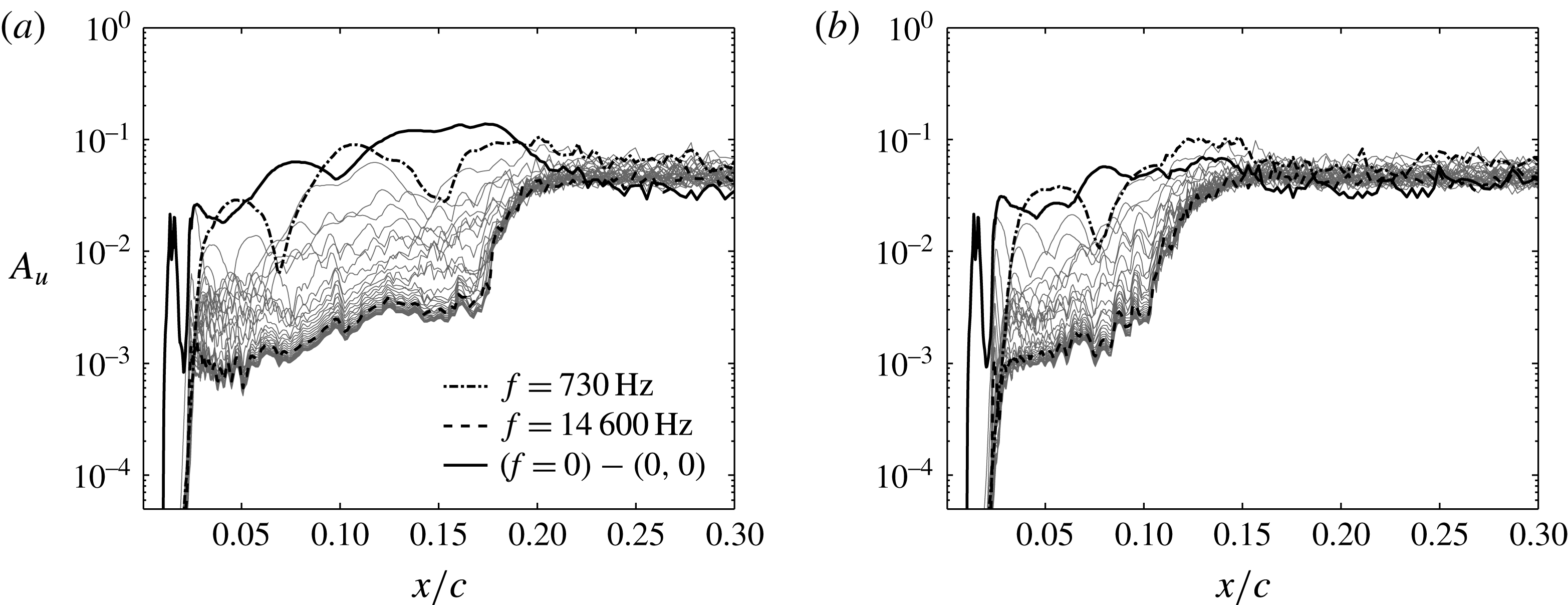
Amplitude evolution of steady and unsteady disturbances for (a) uncontrolled and (b) controlled cases. The grey lines represent unsteady disturbances plotted at a constant frequency step of 730 Hz.

In order to characterise the disturbance environment and the transition mechanism, the total velocity field is decomposed into time-periodic Fourier modes. This will allow us to capture the evolution of both steady and unsteady perturbations. Additionally, the onset of secondary instabilities can be identified by an explosive growth of high-frequency modes similar to the observations in previous studies (Malik et al. Reference Malik, Li, Choudhari and Chang1999; Wassermann & Kloker Reference Wassermann and Kloker2002, Reference Wassermann and Kloker2003; White & Saric Reference White and Saric2005; Hosseini et al. Reference Hosseini, Tempelmann, Hanifi and Henningson2013). To this end, the amplitude of individual cross-flow modes is obtained by means of Fourier transformation in time, i.e.
 $$\begin{eqnarray}\displaystyle u_{\unicode[STIX]{x1D709}}(\unicode[STIX]{x1D709},\unicode[STIX]{x1D702},z,t)=\mathop{\sum }_{m=0}^{M}\tilde{u} _{\unicode[STIX]{x1D709}}(\unicode[STIX]{x1D709},\unicode[STIX]{x1D702},z,m\unicode[STIX]{x1D714}_{0})\text{e}^{\text{i}m\unicode[STIX]{x1D714}_{0}t}. & & \displaystyle\end{eqnarray}$$
The amplitudes of individual modes for both the uncontrolled and controlled cases are plotted in figure 12 as
 $$\begin{eqnarray}\displaystyle A_{u}(x)=\max _{\unicode[STIX]{x1D702},z}\frac{|\tilde{u} _{\unicode[STIX]{x1D709}}|}{Q_{\infty }}, & & \displaystyle\end{eqnarray}$$
where
 $\tilde{u} _{\unicode[STIX]{x1D709}}$
is the time Fourier amplitude of the tangential velocity and
 $Q_{\infty }$
denotes the total free-stream velocity. The amplitude of the steady disturbances is obtained by subtracting the mean flow, i.e. the
 $(0,0)$
mode, from the zero-frequency mode. Owing to the complexity of the set-up, the evolution of the amplitude of disturbances is rather complicated. The amplitudes of steady and low-frequency disturbances are of similar order and, in the controlled case, low-frequency disturbances exhibit even higher amplitudes than the stationary disturbances. The low-frequency disturbances can be associated with unsteady primary cross-flow disturbances (see figure 7).
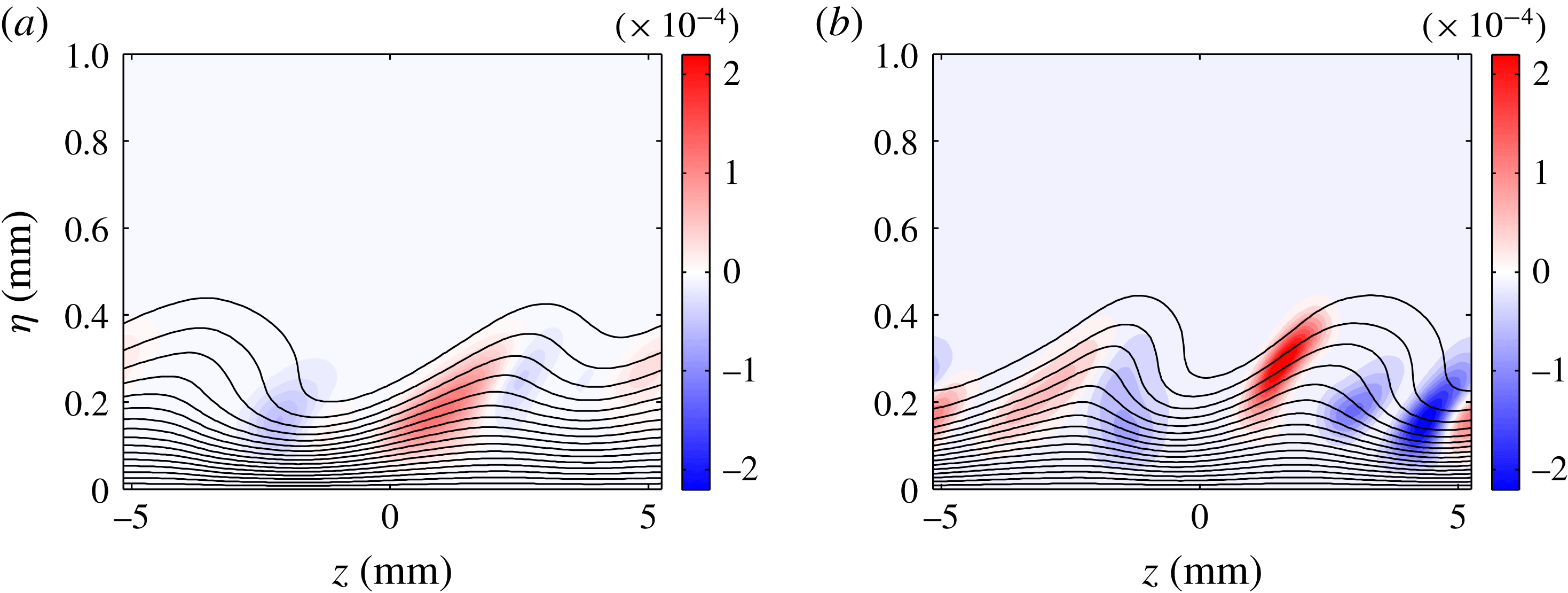
Contours of modified mean flow (tangential component) in black and distribution of the production term
 $-(\tilde{u} _{\unicode[STIX]{x1D709}}^{r}\tilde{w}^{r}+\tilde{u} _{\unicode[STIX]{x1D709}}^{i}\tilde{w}^{i})\unicode[STIX]{x2202}U_{\unicode[STIX]{x1D709}}/\unicode[STIX]{x2202}z$
for the high-frequency mode with frequency 14 600 Hz: (a) uncontrolled case and (b) controlled case. The wall-normal plane is chosen at
 $x/c=0.09$
, located upstream of the transition location in both cases. Contour levels are identical in both cases.

In both cases, the high-frequency disturbances are excited, and just upstream of the transition location they undergo a sudden amplification and reach the amplitude of primary modes within few per cent of the chord length. This is a characteristic behaviour of the secondary instabilities; once the primary cross-flow waves reach high amplitudes, the secondary instabilities are destabilised and grow to large amplitudes over a very short streamwise distance and lead to breakdown and turbulence (White & Saric Reference White and Saric2005). Here, the amplitudes of primary disturbances, both the steady and unsteady ones, reach
 ${\sim}10\,\%$
of the total free-stream velocity prior to transition. Owing to the complex disturbance environment in our set-up, it is not easy to isolate the secondary instability mechanism. Under more controlled conditions, it has been shown that transition is induced by either stationary or travelling saturated cross-flow disturbances (Högberg & Henningson Reference Högberg and Henningson1998; Malik et al.
Reference Malik, Li, Choudhari and Chang1999; Wassermann & Kloker Reference Wassermann and Kloker2002, Reference Wassermann and Kloker2003). Moreover, Lerche (Reference Lerche1996) and Lerche & Bippes (Reference Lerche, Bippes, Henkes and van Ingen1996) observed that a superposition of both stationary and travelling primary modes can destabilise the secondary instability, while individually they are not strong enough to produce sufficient mean-flow deformation and trigger the secondary instability. In this case, the transition is induced by coexisting steady and unsteady cross-flow disturbances that exhibit similar amplitudes.
Based on the production of disturbance energy, secondary instabilities are often categorised into two types (Malik, Li & Chang Reference Malik, Li and Chang1996; Malik et al.
Reference Malik, Li, Choudhari and Chang1999),
 $z$
- and
 $y$
-type modes, which are produced by the spanwise and wall-normal gradients of the mean streamwise velocity, respectively. Figure 13 shows the streamwise velocity component of the modified mean flow along with the distribution of the energy production term associated with a
 $z$
-type mode,
 $-(\tilde{u} _{\unicode[STIX]{x1D709}}^{r}\tilde{w}^{r}+\tilde{u} _{\unicode[STIX]{x1D709}}^{i}\tilde{w}^{i})\unicode[STIX]{x2202}U_{\unicode[STIX]{x1D709}}/\unicode[STIX]{x2202}z$
, for the high-frequency mode with frequency 14 600 Hz. Here, superscripts
 $r$
and
 $i$
indicate the real and imaginary parts of complex amplitudes
 $\tilde{u} _{\unicode[STIX]{x1D709}}$
and
 $\tilde{w}$
. The sign of the production term indicates whether the local transfer of kinetic energy associated with it acts as stabilising (negative) or destabilising (positive). The wall-normal plane
 $(\unicode[STIX]{x1D702},z)$
is chosen at
 $x/c=0.09$
, an upstream position of the transition location for both the uncontrolled and the controlled cases. Although the cross-flow vortices are not saturated in either case, the mean-flow modification by the control mode has resulted in the formation of stronger cross-flow vortices. The maximum of the production is located on the updraught side of the primary vortices with slightly larger values in the controlled case. Therefore, the secondary instabilities are destabilised slightly earlier than in the uncontrolled case, which is followed by promotion of transition to turbulence.
3.4 Improved control and transition delay
In this section we aim to improve the control and delay the transition using ring-type plasma actuators acting as virtual roughness elements. There are several design parameters in this control technique that could be investigated for improvement, i.e. the streamwise location or the spanwise spacing of plasma actuators, and the strength of actuators in terms of the magnitude of the induced velocity (which corresponds to the height of a roughness element). Actuators should be located at streamwise locations where the boundary layer is more receptive to the excitation of the control mode. Here we have positioned the actuators slightly downstream of the neutral point of the stationary cross-flow vortices. The spanwise spacing of the actuators is chosen to be smaller than the spanwise wavelength of the naturally most unstable mode so that the control mode is subcritical with respect to the most amplified mode and decays far downstream. Following the suggestion by Saric et al. (Reference Saric, Ruben and Reibert1998), we have spaced the plasma actuators with a spanwise wavelength equal to two-thirds of the wavelength of the naturally most unstable mode. Saric, Carpenter & Reed (Reference Saric, Carpenter and Reed2008) placed roughness elements at half of the wavelength of the most unstable cross-flow mode in their free-flight experiments, which was found to be effective in delaying transition (see also Saric et al. Reference Saric, Carpenter and Reed2011). Choosing higher harmonics of the most unstable mode is also possible, but the control mode may become too damped and therefore not effective.
In successful applications of this control technique, Wassermann & Kloker (Reference Wassermann and Kloker2002) and Hosseini et al. (Reference Hosseini, Tempelmann, Hanifi and Henningson2013) have shown that the amplitude of the control mode is around one order of magnitude larger than the most unstable stationary mode in the upstream regions of their flow cases (e.g. see figure 3 of the latter study). Furthermore, Wassermann & Kloker (Reference Wassermann and Kloker2002) show that increasing the amplitude of the control mode results in further suppression of the most unstable stationary modes and hence a more effective control (e.g. see their figure 24). Moreover, suppression of unsteady disturbances by nonlinear steady cross-flow modes has been shown by Bonfigli & Kloker (Reference Bonfigli and Kloker1999). In our flow case, the amplitude of the control mode, shown in figure 8(b), is one order of magnitude smaller than the amplitude of the most unstable mode and it is too weak compared to the cases in which control has successfully delayed transition. Therefore, among the design parameters mentioned, we choose to investigate the plasma actuator strength for improvement of the control. To this end, the plasma actuator body force is increased by a factor of 100, which corresponds to increasing the magnitude of the induced jet velocity by a factor of 25 from
 ${\approx}0.2$
to
 ${\approx}5.0~\text{m}~\text{s}^{-1}$
. Note that here we simply assume that the shape of the force field would stay the same when the actuation amplitude is increased. This is an assumption that we could not validate, as we do not have access to data with higher actuation amplitude. The main goal of this exercise is obtaining an idea about the level of jet velocity required for transition delay.
(a) Amplitude evolution
 $A_{u}$
of the stationary modes in the absence of unsteady perturbations for the improved controlled case with higher plasma actuator body force. Circular symbols show the amplitude evolution predicted by nonlinear PSE computation. (b) Amplitude of the total disturbances for the uncontrolled and controlled cases.

Figure 14(a) shows the evolution of the amplitude of the individual stationary cross-flow modes, in the absence of unsteady perturbations, for the new controlled case where the amplitude of the plasma actuator body force is increased. The amplitude of the
 $3\unicode[STIX]{x1D6FD}_{0}$
mode after excitation by the plasma actuator experiences a sharp increase and becomes the dominant mode. Farther downstream, at approximately
 $x/c\approx 0.21$
, it becomes stable and decays. The qualitative behaviour of the control mode in this case is similar to those reported by Wassermann & Kloker (Reference Wassermann and Kloker2002) and Hosseini et al. (Reference Hosseini, Tempelmann, Hanifi and Henningson2013). The evolution of the amplitude of the total disturbances for both the uncontrolled and controlled cases is shown in figure 14(b). Unlike the previous controlled case, shown in figure 9(b), excitation of the control mode leads to total disturbance amplitudes that are three times higher than those of the uncontrolled case. However, far downstream at approximately
 $x/c\approx 0.21$
it decays, and for
 $x/c>0.23$
the total amplitude level is slightly below that of the uncontrolled case.
(a) Time-averaged friction coefficient for the uncontrolled and the improved controlled case. (b) Amplitude evolution of steady and unsteady disturbances for the improved controlled case with higher plasma actuator body force. The grey lines represent unsteady disturbances plotted at a constant frequency step of 730 Hz.

In order to evaluate the control capability of the plasma actuators with stronger body force in a realistic more complex disturbance environment, unsteady perturbations are introduced in the domain. The unsteady volume force is kept the same as in the previous section. Figure 15(a) shows the time-averaged friction coefficient for both the uncontrolled and controlled cases. It is clear that the new control has delayed the transition to turbulent flow by approximately 3 % chord length. However, owing to differences between the modelled and the actual perturbation field in the wind tunnel, this value might be different in the real case. The Fourier transform of flow field snapshots in time characterises the disturbance environment into steady and unsteady parts. The amplitude of the individual modes, as defined in (3.5), for the controlled case are plotted in figure 15(b). The steady disturbances are clearly dominant in this controlled case. The initial amplitudes of unsteady perturbations, both primary and secondary, are similar to those in the uncontrolled case up to the location of plasma actuators at
 $x/c=0.05$
. Thereafter, they experience a sharp decay up to
 $x/c\approx 0.1$
, where they start to grow again. However, the unsteady disturbances are attenuated compared to the uncontrolled case. Furthermore, the sudden growth of high-frequency disturbances is shifted downstream, which corresponds to the beginning of the transition location in the friction coefficient curve.
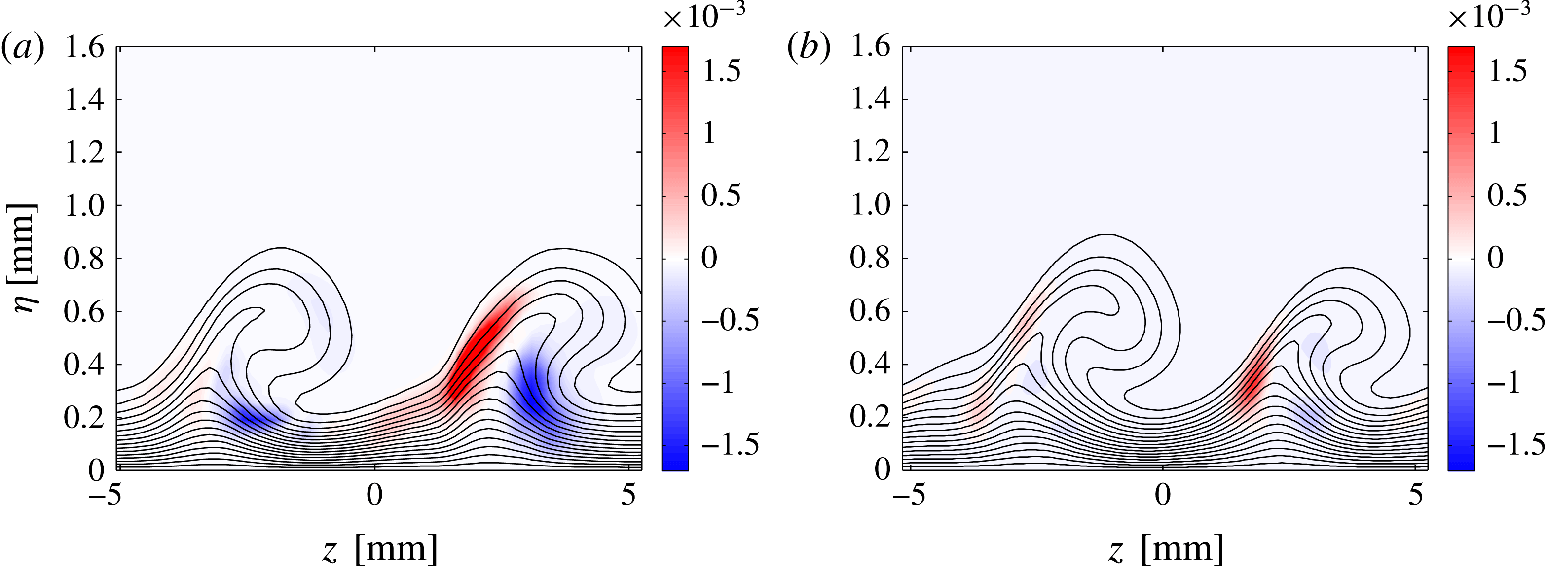
Spatial distribution of the production term
 $-(\tilde{u} _{\unicode[STIX]{x1D709}}^{r}\tilde{w}^{r}+\tilde{u} _{\unicode[STIX]{x1D709}}^{i}\tilde{w}^{i})\unicode[STIX]{x2202}U_{\unicode[STIX]{x1D709}}/\unicode[STIX]{x2202}z$
for the high-frequency mode with frequency 14 600 Hz along with contours of modified mean flow (tangential velocity component): (a) uncontrolled case and (b) controlled case. The wall-normal
 $(\unicode[STIX]{x1D702},z)$
plane is located at
 $x/c=0.17$
.

In order to understand further the mechanism of secondary instabilities, the transfer of energy between the base flow and the high-frequency modes is investigated. To this end, the spatial distribution of the energy production term associated with
 $z$
-type modes,
 $-(\tilde{u} _{\unicode[STIX]{x1D709}}^{r}\tilde{w}^{r}+\tilde{u} _{\unicode[STIX]{x1D709}}^{i}\tilde{w}^{i})\unicode[STIX]{x2202}U_{\unicode[STIX]{x1D709}}/\unicode[STIX]{x2202}z$
, along with contours of the modified mean flow is shown in figure 16. As the secondary instability scales with strength of the spanwise shear, same trend is usually observed for all secondary modes when the strength of cross-flow modes is varied. This is confirmed by comparing figures 15(b) and 12(a); the amplitude for the whole range of the secondary modes is decreased in the case of high-amplitude forcing. Therefore, we compare the secondary disturbances with the same frequency (
 $f=14\,600~\text{Hz}$
) in both uncontrolled and controlled cases. The wall-normal plane is chosen at
 $x/c=0.17$
, prior to the transition location in both the controlled and uncontrolled cases. The maximum production is located on the upwelling zone of the stationary cross-flow vortices where the shear is strong. The destabilising energy production is clearly weaker in the controlled case as compared with the uncontrolled case. Although figure 14(a) shows the dominance of the control mode in the absence of unsteady disturbances, the mean-flow structure in both the uncontrolled and controlled cases is dominated by the most unstable
 $2\unicode[STIX]{x1D6FD}_{0}$
mode in the presence of unsteady perturbations. In order to investigate this behaviour, the disturbances are assumed to be spanwise and time periodic and may be decomposed into Fourier components of the form
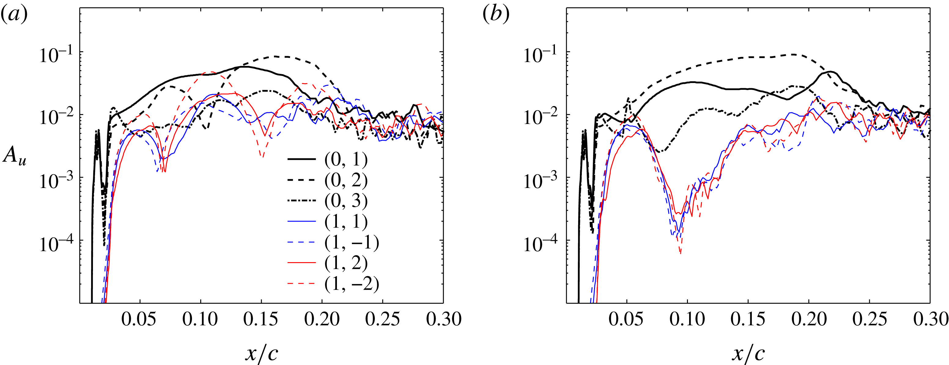
 $$\begin{eqnarray}\displaystyle u_{\unicode[STIX]{x1D709}}(\unicode[STIX]{x1D709},\unicode[STIX]{x1D702},z,t)=\mathop{\sum }_{m=0}^{M}\mathop{\sum }_{n=-N}^{N}{\check{u}}_{\unicode[STIX]{x1D709}}(\unicode[STIX]{x1D709},\unicode[STIX]{x1D702},n\unicode[STIX]{x1D6FD}_{0},m\unicode[STIX]{x1D714}_{0})\text{e}^{\text{i}(n\unicode[STIX]{x1D6FD}_{0}z+m\unicode[STIX]{x1D714}_{0}t)}. & & \displaystyle\end{eqnarray}$$
The amplitudes of individual modes for both the uncontrolled and controlled cases are plotted in figure 17 as
 $$\begin{eqnarray}\displaystyle A_{u}(x)=\max _{\unicode[STIX]{x1D702}}\frac{|{\check{u}}_{\unicode[STIX]{x1D709}}|}{Q_{\infty }}. & & \displaystyle\end{eqnarray}$$
In the following, individual Fourier modes with a spanwise wavenumber
 $n\unicode[STIX]{x1D6FD}_{0}$
and a frequency
 $m\unicode[STIX]{x1D714}_{0}$
are represented by
 $(m,n)$
. The fundamental frequency resolved here is
 $f_{0}=2\unicode[STIX]{x03C0}\unicode[STIX]{x1D714}_{0}=730~\text{Hz}$
. In the uncontrolled case, steady and unsteady disturbances exhibit similar amplitude levels, with the
 $(0,1)$
mode being dominant up to
 $x/c\approx 0.13$
where the
 $(0,2)$
mode becomes dominant. In the controlled case, excitation of the control mode clearly attenuates the unsteady modes as well as the
 $(0,1)$
mode. The dominant mode throughout the domain is the
 $(0,2)$
mode in contrast to dominance of the control
 $(0,3)$
mode in the purely steady disturbance environment. This demonstrates the significant effect of unsteady disturbances in the receptivity process.
Amplitude evolution of primary modes for (a) uncontrolled and (b) controlled cases, obtained using spatio-temporal Fourier decomposition of disturbances.

4 Conclusions
Control of a swept-wing boundary layer using ring-type plasma actuators is investigated thorough direct numerical simulations. The flow configuration conforms to experiments by Kim et al. (Reference Kim, Forte and Choi2016) in which a spanwise array of ring-type plasma actuators were mounted close to the leading edge. Such actuators generate a wall-normal jet and act as virtual roughness elements to excite subcritical stationary control modes. The action of actuators is incorporated in the numerical simulations by including the corresponding body force of the induced velocity field by actuators. Steady cross-flow disturbances are excited using a simplified model of surface roughness on the wing surface.
First, the effect of control on the evolution of stationary cross-flow disturbances in the absence of unsteady perturbations is investigated, i.e. transition is not studied. Excitation of the control mode attenuates the amplitude of the most unstable mode as well as the total amplitude of stationary disturbances. The amplitude of the dominant mode in both the uncontrolled and controlled cases is rather low and not saturated within the computational domain. In the next step, a more realistic disturbance environment is considered by adding unsteady disturbances in the leading-edge region using random volume force in the wall-normal direction. The amplitude of unsteady perturbations is adjusted such that the transition location is close to the experimental one. Employing control in this set-up leads to promotion of transition, which is in qualitative agreement with the experimental observations. The breakdown from laminar to turbulent flow is caused by the explosive growth of the secondary instability modes. In both the uncontrolled and controlled cases, stationary and travelling cross-flow modes exhibit similar amplitudes, and a combination of both modes triggers the secondary instabilities.
An improvement in the control is demonstrated by employing stronger plasma actuators with one order of magnitude larger jet velocity. Note that here we simply assume that the shape of the force field would stay the same when actuation amplitude is increased. This is an assumption that we could not validate, as we do not have access to data with higher actuation amplitude. In the absence of unsteady perturbations, the amplitude of the control mode for such a plasma actuator initially dominates the amplitude of the stationary modes and decays far downstream. This behaviour is in qualitative agreement with previous studies (e.g. Wassermann & Kloker Reference Wassermann and Kloker2002; Hosseini et al.
Reference Hosseini, Tempelmann, Hanifi and Henningson2013). It is shown that employing stronger plasma actuators in a disturbance environment with both steady and unsteady perturbations successfully delays transition. Note that the location of the actuators in the simulations (
 $x/c=0.05$
) is different from those in the experiments (
 $x/c=0.019$
) and therefore the efficiency of the actuation may be different there. It is observed that the amplitude of the unsteady disturbances, both the primary and the secondary, is attenuated when the control is applied. However, the modified mean flow is still dominant by the naturally most unstable cross-flow mode. This is confirmed by spatio-temporal Fourier decomposition of the disturbances. The results of the simulations show a complex interaction between stationary and unsteady vortices indicating the importance of unsteady cross-flow vortices in the transition for the case under consideration.
Acknowledgements
The authors would like to thank P. Dörr for fruitful discussions and valuable comments. This work has been supported by the European Commission through FP7 project BUTERFLI (grant agreement no. ACP3-GA-2013-605605). Computer time provided by SNIC (Swedish National Infrastructure for Computing) is gratefully acknowledged.