1 Introduction
Thermal transport in shear flows is a fundamental problem in fluid mechanics that arises in many engineering and geophysical situations. It combines phenomena in fluid layers without external shear (the Rayleigh–Bénard (RB) flow (Chandrasekhar Reference Chandrasekhar1961)) and in shear flows without heating (Grossmann Reference Grossmann2000; Schmid & Henningson Reference Schmid and Henningson2001). The onset of convection in the RB setting has been studied in considerable detail in various geometries (Busse Reference Busse1978). The properties of shear flows are less well understood because of the difficulties presented by the manner in which they become turbulent (Grossmann Reference Grossmann2000; Schmid & Henningson Reference Schmid and Henningson2001). In contrast to RB flows, turbulence in shear flows is often observed when the laminar profile is still linearly stable, so that the transition requires finite-amplitude perturbations that reach states that arise in subcritical bifurcations (Eckhardt et al. Reference Eckhardt, Schneider, Hof and Westerweel2007). The advective nature and the spatial development in open boundary layers add to the complexity.
The interaction between shear and convection has been studied in boundary layers (Sparrow & Cess Reference Sparrow and Cess1961; Merkin Reference Merkin1972), where it affects the functional form of the profile (Marati et al. Reference Marati, Davoudi, Casciola and Eckhardt2006). The dynamics of plumes and other structures has been investigated in the context of RB flows (Ahlers, Grossmann & Lohse Reference Ahlers, Grossmann and Lohse2009; Chillà & Schumacher Reference Chillà and Schumacher2012) because of their contribution to the heat transport (Zocchi, Moses & Libchaber Reference Zocchi, Moses and Libchaber1990; Parodi et al. Reference Parodi, von Hardenberg, Passoni, Provenzale and Spiegel2004; Zhou, Sun & Xia Reference Zhou, Sun and Xia2007; Zhou & Xia Reference Zhou and Xia2010). The presence of instabilities is connected with a transition that also marks the entry into the ultimate regime (Grossmann & Lohse Reference Grossmann and Lohse2000a , Reference Grossmann and Lohse2002). Experiments by Du Puits et al. (Reference Du Puits, Li, Resagk, Thess and Willert2013) show that the flow in the transition region can be spatially localized and transient, very much as in the case of bypass transition in shear flows. A quantitative study focusing on the hydrodynamic instabilities in heated boundary layers does not seem to have been published.
The manner in which shear and buoyancy interact to shape the transition has been studied by Clever & Busse (Reference Clever and Busse1992) for the case of RB with a linear shear. They identified the onset of modulated rolls and the transition to a subcritical regime when the shear was strong and the temperature gradient weak. Ultimately, this state could be traced to an exact coherent structure (ECS) in plane Couette flow that is related to the transition in the pure shear flow without a temperature gradient. The ECS reached via heating coincides with the one obtained by adding rotation as a destabilizing force (Nagata Reference Nagata1990). Using these and related embeddings, as well as some other techniques (Dijkstra et al. Reference Dijkstra, Wubs, Cliffe, Doedel, Dragomirescu, Eckhardt, Gelfgat, Hazel, Lucarini and Salinger2014), numerous exact coherent structures have been identified in plane Couette flow (Nagata Reference Nagata1990; Schmiegel Reference Schmiegel1999; Gibson, Halcrow & Cvitanović Reference Gibson, Halcrow and Cvitanović2009), in pipe flow (Faisst & Eckhardt Reference Faisst and Eckhardt2003; Hof et al. Reference Hof, van Doorne, Westerweel, Nieuwstadt, Faisst, Eckhardt, Wedin, Kerswell and Waleffe2004; Wedin & Kerswell Reference Wedin and Kerswell2004; Pringle & Kerswell Reference Pringle and Kerswell2007; Duguet, Pringle & Kerswell Reference Duguet, Pringle and Kerswell2008; Eckhardt et al. Reference Eckhardt, Faisst, Schmiegel and Schneider2008), in plane Poiseuille flow (Waleffe Reference Waleffe2001; Nagata & Deguchi Reference Nagata and Deguchi2013; Gibson & Brand Reference Gibson and Brand2014; Zammert & Eckhardt Reference Zammert and Eckhardt2014a ,Reference Zammert and Eckhardt b ) and even in boundary layers (Duguet et al. Reference Duguet, Schlatter, Henningson and Eckhardt2012). For these flows the observed transient subcritical turbulence could be explained by ECS which create a chaotic saddle in a series of bifurcations (Kreilos & Eckhardt Reference Kreilos and Eckhardt2012; Avila et al. Reference Avila, Mellibovsky, Roland and Hof2013; Zammert & Eckhardt Reference Zammert and Eckhardt2015). Further studies have shown that ECS are linked dynamically (Halcrow et al. Reference Halcrow, Gibson, Cvitanović and Viswanath2009) and embedded in the turbulent dynamics (Kawahara & Kida Reference Kawahara and Kida2001).
The asymptotic suction boundary layer (ASBL) (Schlichting & Gersten Reference Schlichting and Gersten1997) is a boundary layer that is of interest on its own because of its relation to flow control since suction stabilizes the boundary layer. It is also of theoretical interest since the flow is parallel and can hence be studied using the tools developed for parallel shear flows. Experimental realizations of both the pure shear flow (Fransson & Alfredsson Reference Fransson and Alfredsson2003) and the heated version (Moffat & Kays Reference Moffat and Kays1968) are available. Taking the cross-flow as a parameter, the ECS from plane Couette flow could be traced to ASBL and a transition in the dynamics could be identified (Kreilos et al. Reference Kreilos, Veble, Schneider and Eckhardt2013; Kreilos, Gibson & Schneider Reference Kreilos, Gibson and Schneider2016). Further ECS for ASBL, in the form of travelling waves and periodic orbits, have been identified and studied (Khapko et al. Reference Khapko, Kreilos, Schlatter, Duguet, Eckhardt and Henningson2013, Reference Khapko, Duguet, Kreilos, Schlatter, Eckhardt and Henningson2014; Deguchi & Hall Reference Deguchi and Hall2014). We here expand the analysis of the ASBL to include heating of the bottom plate, so as to form a thermal asymptotic suction boundary layer (TASBL). The study of such a parallel TASBL contributes to our understanding of the turbulence transition and the dynamics of coherent structures in thermal boundary layers.
The further outline of this paper is as follows: in § 2, we introduce the system and its laminar solution. The stability of the base flow as a function of Rayleigh number, Reynolds number and Prandtl number and the two-dimensional secondary solutions bifurcating from the laminar state are discussed in § 3. In § 4 examples of the cascade of bifurcations that lead to a chaotic saddle and subcritical chaos in the system are studied. Finally, in § 5 three-dimensional secondary bifurcations are analysed, with a particular emphasis on exact solutions that are localized in both directions parallel to the plate. We end with an outlook in § 6.
2 Description of the system and its laminar state
The asymptotic suction boundary layer is the flow over a plate through which fluid is sucked homogeneously with a speed
 $-V_{S}$
. Far above the plate, the parallel velocity component of the flow has a speed
 $U_{\infty }$
. For TASBL there is a temperature difference
 $T_{0}$
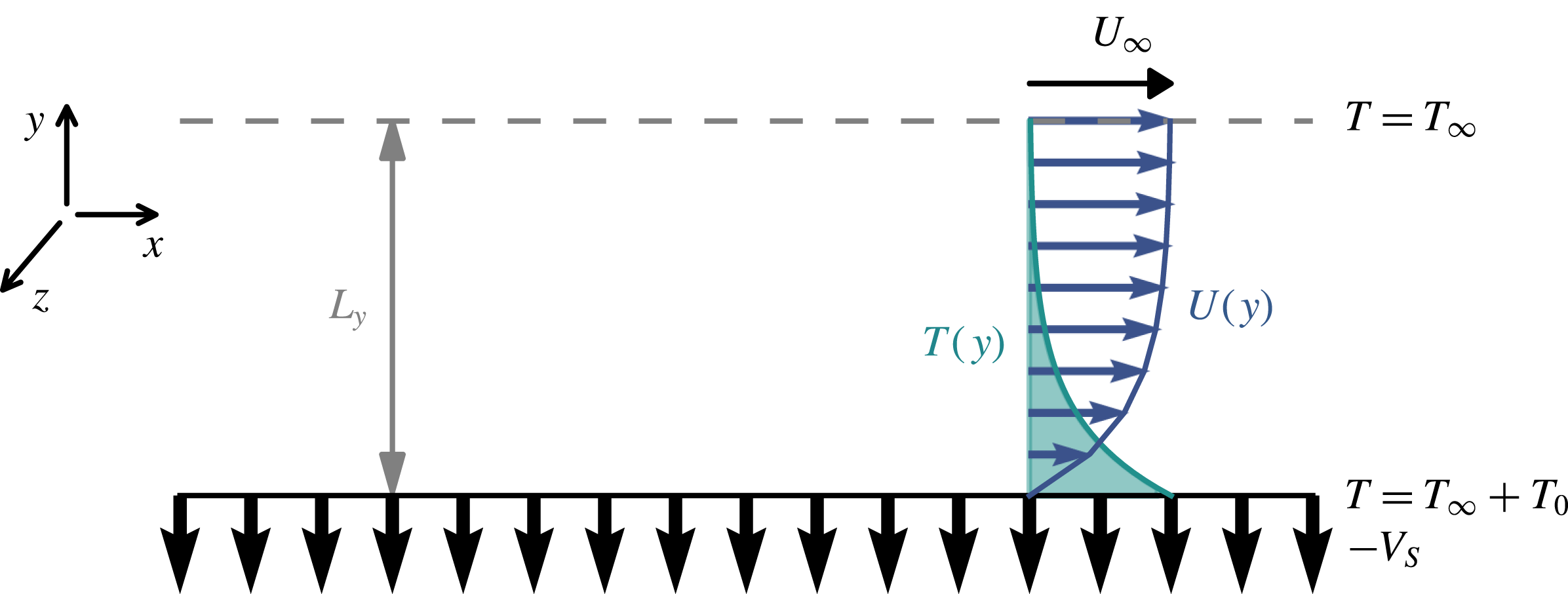
between the plate and the fluid far above the plate. The flow geometry of TASBL is sketched in figure 1.
Sketch of the ASBL over a heated plate. Far above the plate the flow moves with speed
 $U_{\infty }$
in the streamwise direction. The temperature difference between the plate and the fluid far above the plate is
 $T_{0}$
. In the numerical simulation the domain is closed from above with a plate at a height
 $L_{y}$
, indicated by a grey line.

The flow is governed by the Overbeck–Boussinesq equations (Landau & Lifschitz Reference Landau and Lifschitz1959)
 $$\begin{eqnarray}\displaystyle & \displaystyle \unicode[STIX]{x2202}_{t}\boldsymbol{u}+(\boldsymbol{u}\boldsymbol{\cdot }\unicode[STIX]{x1D735})\boldsymbol{u}=-\unicode[STIX]{x1D735}p+\unicode[STIX]{x1D708}\unicode[STIX]{x0394}\boldsymbol{u}+\unicode[STIX]{x1D6FD}g\unicode[STIX]{x1D703}\boldsymbol{e}_{y}, & \displaystyle\end{eqnarray}$$
 $$\begin{eqnarray}\displaystyle & \displaystyle \unicode[STIX]{x2202}_{t}\unicode[STIX]{x1D703}+(\boldsymbol{u}\boldsymbol{\cdot }\unicode[STIX]{x1D735})\unicode[STIX]{x1D703}=\unicode[STIX]{x1D705}\unicode[STIX]{x0394}\unicode[STIX]{x1D703}, & \displaystyle\end{eqnarray}$$
 $$\begin{eqnarray}\displaystyle & \displaystyle \unicode[STIX]{x0394}\boldsymbol{u}=0, & \displaystyle\end{eqnarray}$$
where
 $\unicode[STIX]{x1D708}$
is the kinematic viscosity,
 $\unicode[STIX]{x1D705}$
the thermal diffusivity,
 $\unicode[STIX]{x1D6FD}$
the thermal expansion coefficient and
 $g$
the gravitational acceleration, pointing in the
 $y$
-direction perpendicular to the plate. The boundary conditions of the system are
 $$\begin{eqnarray}u(y=0)=0\quad \text{and}\quad u(y=\infty )=U_{\infty },\end{eqnarray}$$
 $$\begin{eqnarray}v(y=0)=v(y=\infty )=-V_{S},\end{eqnarray}$$
 $$\begin{eqnarray}\unicode[STIX]{x1D703}(y=0)=T_{0}\quad \text{and}\quad \unicode[STIX]{x1D703}(y=\infty )=0.\end{eqnarray}$$
The stationary laminar profile for the velocity is given by
 $$\begin{eqnarray}\boldsymbol{U}(x,y,z)=(U(y),-V_{s},0)\quad \text{with}~U(y)=U_{\infty }(1-\text{e}^{-V_{s}y/\unicode[STIX]{x1D708}})\end{eqnarray}$$
and the deviation of the temperature from the background temperature
 $T_{\infty }$
is given by
 $$\begin{eqnarray}T(x,y,z)=T_{0}\cdot \text{e}^{-V_{s}y/\unicode[STIX]{x1D705}}.\end{eqnarray}$$
A characteristic length scale of the system is the displacement thickness (Schlichting & Gersten Reference Schlichting and Gersten1997)
 $$\begin{eqnarray}\unicode[STIX]{x1D6FF}=\int _{0}^{\infty }\left(1-\frac{U(y)}{U_{\infty }}\right)\text{d}y=\frac{\unicode[STIX]{x1D708}}{V_{S}}.\end{eqnarray}$$
The dimensionless numbers characterizing the system are the Reynolds, Prandtl and Rayleigh number, given by
 $$\begin{eqnarray}\mathit{Re}=\frac{U_{\infty }\unicode[STIX]{x1D6FF}}{\unicode[STIX]{x1D708}}=\frac{U_{\infty }}{V_{s}},\quad \mathit{Pr}=\frac{\unicode[STIX]{x1D708}}{\unicode[STIX]{x1D705}},\quad \mathit{Ra}=\frac{\unicode[STIX]{x1D6FD}g\unicode[STIX]{x1D6FF}^{3}T_{0}}{\unicode[STIX]{x1D705}\unicode[STIX]{x1D708}}.\end{eqnarray}$$
The equations can be made dimensionless by measuring lengths in units of
 $\unicode[STIX]{x1D6FF}$
, time in units of
 $\unicode[STIX]{x1D6FF}^{2}/\unicode[STIX]{x1D705}$
(corresponding to measuring velocities in units of
 $\unicode[STIX]{x1D705}/\unicode[STIX]{x1D6FF}$
) and temperature in units of
 $T_{0}/\mathit{Ra}$
:
 $$\begin{eqnarray}\displaystyle & \displaystyle \unicode[STIX]{x2202}_{t}\boldsymbol{u}+(\boldsymbol{u}\boldsymbol{\cdot }\unicode[STIX]{x1D735})\boldsymbol{u}=-\unicode[STIX]{x1D735}p+Pr\,\unicode[STIX]{x0394}\boldsymbol{u}+\mathit{Pr}\,\mathit{Ra}\,\unicode[STIX]{x1D703}\boldsymbol{e}_{y}, & \displaystyle\end{eqnarray}$$
 $$\begin{eqnarray}\displaystyle & \displaystyle \unicode[STIX]{x2202}_{t}\unicode[STIX]{x1D703}+(\boldsymbol{u}\boldsymbol{\cdot }\unicode[STIX]{x1D735})\unicode[STIX]{x1D703}=\unicode[STIX]{x0394}\unicode[STIX]{x1D703}, & \displaystyle\end{eqnarray}$$
 $$\begin{eqnarray}\displaystyle & \displaystyle \unicode[STIX]{x1D735}\boldsymbol{\cdot }\boldsymbol{u}=0. & \displaystyle\end{eqnarray}$$
The non-dimensionalized laminar profiles become
 $$\begin{eqnarray}\boldsymbol{U}(x,y,z)=(U(y),-Pr,0),\quad U(y)=\mathit{Pr}\,\mathit{Re}(1-\text{e}^{-y}),\end{eqnarray}$$
 $$\begin{eqnarray}T(x,y,z)=\mathit{Ra}\,\text{e}^{-Pr\,y}.\end{eqnarray}$$
The thickness
 $\unicode[STIX]{x1D6FF}_{\unicode[STIX]{x1D703}}$
of the thermal boundary layer is then inversely proportional to the Prandtl number,
 $$\begin{eqnarray}\unicode[STIX]{x1D6FF}_{\unicode[STIX]{x1D703}}=\frac{\unicode[STIX]{x1D6FF}}{\mathit{Pr}}.\end{eqnarray}$$
Thus, the Prandtl number can also be interpreted as the ratio between the thicknesses of the velocity boundary layer
 $\unicode[STIX]{x1D6FF}$
and the thermal boundary layer
 $\unicode[STIX]{x1D6FF}_{\unicode[STIX]{x1D703}}$
. For values of
 $\mathit{Pr}$
smaller than unity (e.g. air and liquid metals) the thermal boundary layer is thicker than the velocity boundary layer. For
 $\mathit{Pr}=1$
both have the same thickness, while for
 $\mathit{Pr}>1$
(e.g. water and oils) the thermal boundary layer is the thinner one.
The velocity and temperature fields are decomposed into a base flow and fluctuations,
 $$\begin{eqnarray}\displaystyle & \displaystyle \unicode[STIX]{x1D703}=T+\unicode[STIX]{x1D703}^{\prime }, & \displaystyle\end{eqnarray}$$
 $$\begin{eqnarray}\displaystyle & \displaystyle \boldsymbol{u}=\boldsymbol{U}+\boldsymbol{u}^{\prime }. & \displaystyle\end{eqnarray}$$
Unless stated explicitly, only the fluctuations
 $\unicode[STIX]{x1D703}^{\prime }$
and
 $\boldsymbol{u}^{\prime }$
are visualized or used in bifurcation diagrams.
In the numerical simulations the wall-normal direction has to be truncated at some distance
 $L_{y}$
. To this end, the system is closed with a permeable plate with asymptotic temperature and velocity components, and no-slip boundary conditions for the deviations. The modified base profiles become
 $$\begin{eqnarray}U^{\ast }(y)=\mathit{Re}\,\mathit{Pr}\frac{1-\text{e}^{-y}}{1-\text{e}^{-L_{y}}}\end{eqnarray}$$
and
 $$\begin{eqnarray}T^{\ast }(y)=\frac{\mathit{Ra}}{1-\text{e}^{-Pr\,L_{y}}}(\text{e}^{-Pr\,y}-\text{e}^{-Pr\,L_{y}}).\end{eqnarray}$$
In all simulations a value of
 $L_{y}$
equal to or larger than
 $20$
is used. In all simulations it was carefully checked that this value was sufficiently big so that the differences between the asymptotic profiles
 $U(y)$
and
 $T(y)$
and the finite profiles
 $U^{\ast }(y)$
and
 $T^{\ast }(y)$
remained small.
A quantity of particular interest in the study of thermal systems is the heat flux, which has a convective and a conductive contribution. For the base flow, the convective heat flux is given by
 $$\begin{eqnarray}\unicode[STIX]{x1D719}_{conv}(y)=\langle v\cdot T\rangle _{x,z}=-Pr\,Ra\,\text{e}^{-Pr\,y}.\end{eqnarray}$$
For the conductive heat flux we find
 $$\begin{eqnarray}\unicode[STIX]{x1D719}_{cond}(y)=-\unicode[STIX]{x2202}_{y}\langle T\rangle _{x,z}=Pr\,Ra\,\text{e}^{-Pr\,y}.\end{eqnarray}$$
Thus, in contrast to Rayleigh–Bénard convection, the conductive heat flux of the base flow depends on the wall-normal coordinate
 $y$
. Moreover, the conductive and convective contributions cancel, and the total heat transfer of the laminar state vanishes. This is no longer the case for the turbulent states. As a dimensionless measure for the heat flux we introduce the Nusselt number
 $Nu$
, the ratio of the total heat flux to the conductive heat flux of the base flow at the wall
 $\unicode[STIX]{x1D719}_{cond}(0)$
,
 $$\begin{eqnarray}\displaystyle Nu & = & \displaystyle \frac{\unicode[STIX]{x1D719}_{conv}+\unicode[STIX]{x1D719}_{cond}}{\unicode[STIX]{x1D719}_{cond}(0)}\end{eqnarray}$$
 $$\begin{eqnarray}\displaystyle & = & \displaystyle \frac{\langle (-Pr+v)(\unicode[STIX]{x1D703}^{\prime }+T)\rangle _{x,z}-\unicode[STIX]{x2202}_{y}\langle \unicode[STIX]{x1D703}^{\prime }+T\rangle _{x,z}}{Pr\,Ra}.\end{eqnarray}$$
In order to eliminate the dependence on the wall-normal coordinate, we integrate over
 $y$
and introduce
 $$\begin{eqnarray}\tilde{\mathit{Nu}}=\int _{0}^{\infty }\mathit{Nu}(y)\,\text{d}y,\end{eqnarray}$$
the volume-integrated heat flux.
3 Stability analysis and secondary solutions
In this section the stability of the laminar state is analysed and the bifurcating secondary solutions are discussed. The linear stability of the flow is determined by solving the Orr–Sommerfeld equations for the flow. The derivation of the equations follows the usual steps and is described in § 3.1. Direct numerical simulation is used to identify exact solutions of the equations. For the simulations we used the Channelflow-code (Gibson Reference Gibson2012) (www.channelflow.org), which we enhanced to handle a temperature field. Details of the modification are given in appendix A.
Following the derivation of the stability equations, we will first analyse the case
 $\mathit{Ra}=0$
in § 3.2. Afterwards, we will present the result for the case
 $\mathit{Re}=0$
in § 3.3. Finally, the combined effect of temperature and shear is discussed in § 3.4.
3.1 Orr–Sommerfeld stability equations
Starting point for the stability analysis are the Navier–Stokes equations (2.11)–(2.13). The full flow field
 $\boldsymbol{u}$
can be expressed as a sum of a base flow contribution
 $\boldsymbol{U}$
and a perturbation
 $\boldsymbol{u}^{\prime }$
. The temperature and pressure fields can be decomposed similarly. Inserting this ansatz in the equations and neglecting the nonlinear terms in the perturbations we obtain:
 $$\begin{eqnarray}\displaystyle & \displaystyle \frac{1}{\mathit{Pr}}[\unicode[STIX]{x2202}_{t}\boldsymbol{u}^{\prime }+(\boldsymbol{u}^{\prime }\boldsymbol{\cdot }\unicode[STIX]{x1D735})\boldsymbol{U}+(\boldsymbol{U}\boldsymbol{\cdot }\unicode[STIX]{x1D735})\boldsymbol{u}^{\prime }]=-\unicode[STIX]{x1D735}p+\unicode[STIX]{x0394}\boldsymbol{u}^{\prime }+\mathit{Ra}(T+\unicode[STIX]{x1D703}^{\prime })\boldsymbol{e}_{y}, & \displaystyle\end{eqnarray}$$
 $$\begin{eqnarray}\displaystyle & \displaystyle \unicode[STIX]{x2202}_{t}\unicode[STIX]{x1D703}^{\prime }+(\boldsymbol{u}^{\prime }\boldsymbol{\cdot }\unicode[STIX]{x1D735})T+\boldsymbol{U}\boldsymbol{\cdot }\unicode[STIX]{x1D735}\unicode[STIX]{x1D703}^{\prime }=\unicode[STIX]{x0394}\unicode[STIX]{x1D703}^{\prime }. & \displaystyle\end{eqnarray}$$
Form this set of equations the pressure can be removed by writing the solenoidal perturbation velocity field
 $\boldsymbol{u}^{\prime }$
in terms of two scalar fields
 $\unicode[STIX]{x1D6F7}(\boldsymbol{x})$
and
 $\unicode[STIX]{x1D6F9}(\boldsymbol{x})$
.
 $$\begin{eqnarray}\boldsymbol{u}^{\prime }=\unicode[STIX]{x1D735}\times \unicode[STIX]{x1D6F9}\boldsymbol{e}_{y}+\unicode[STIX]{x1D735}\times (\unicode[STIX]{x1D735}\times \unicode[STIX]{x1D6F7}\boldsymbol{e}_{y}).\end{eqnarray}$$
For the resulting three scalar fields
 $\unicode[STIX]{x1D6F7}$
,
 $\unicode[STIX]{x1D6F9}$
and
 $\unicode[STIX]{x1D703}^{\prime }$
we take Fourier series in spanwise and streamwise directions and an exponential dependence in time,
 $$\begin{eqnarray}\displaystyle & \displaystyle \unicode[STIX]{x1D6F7}(\boldsymbol{x},t)=\mathop{\sum }_{k_{x},k_{z},\unicode[STIX]{x1D70E}}\unicode[STIX]{x1D6F7}_{k_{x},k_{z},\unicode[STIX]{x1D70E}}(y)\exp (\text{i}(k_{x}x+k_{z}z)+\unicode[STIX]{x1D70E}t), & \displaystyle\end{eqnarray}$$
 $$\begin{eqnarray}\displaystyle & \displaystyle \unicode[STIX]{x1D6F9}(\boldsymbol{x},t)=\mathop{\sum }_{k_{x},k_{z},\unicode[STIX]{x1D70E}}\unicode[STIX]{x1D6F9}_{k_{x},k_{z},\unicode[STIX]{x1D70E}}(y)\exp (\text{i}(k_{x}x+k_{z}z)+\unicode[STIX]{x1D70E}t), & \displaystyle\end{eqnarray}$$
 $$\begin{eqnarray}\displaystyle & \displaystyle \unicode[STIX]{x1D703}^{\prime }(\boldsymbol{x},t)=\mathop{\sum }_{k_{x},k_{z},\unicode[STIX]{x1D70E}}\unicode[STIX]{x1D6E9}_{k_{x},k_{z},\unicode[STIX]{x1D70E}}(y)\exp (\text{i}(k_{x}x+k_{z}z)+\unicode[STIX]{x1D70E}t). & \displaystyle\end{eqnarray}$$
Using this representation of the fields, we obtain the stability equations
 $$\begin{eqnarray}\displaystyle & \displaystyle \left(\frac{\unicode[STIX]{x1D70E}}{Pr}+\frac{\text{i}k_{x}U}{Pr}-D_{y}-(D_{y}^{2}-k^{2})\right)\unicode[STIX]{x1D6F9}(y)+\frac{\text{i}k_{z}U^{\prime }}{Pr}\unicode[STIX]{x1D6F7}(y)=0, & \displaystyle\end{eqnarray}$$
 $$\begin{eqnarray}\displaystyle & \displaystyle \left[\left(\frac{\unicode[STIX]{x1D70E}}{Pr}+\frac{\text{i}k_{x}U}{Pr}-D_{y}\right)(D_{y}^{2}-k^{2})-\frac{\text{i}k_{x}U^{\prime \prime }}{Pr}-(D_{y}^{2}-k^{2})^{2}\right]\unicode[STIX]{x1D6F7}(y)+Ra\unicode[STIX]{x1D6E9}(y)=0, & \displaystyle\end{eqnarray}$$
 $$\begin{eqnarray}\displaystyle & \displaystyle (\unicode[STIX]{x1D70E}+\text{i}k_{x}U-Pr\,D_{y}-(D_{y}^{2}-k^{2}))\unicode[STIX]{x1D6E9}(y)+k^{2}T^{\prime }\unicode[STIX]{x1D6F7}(y)=0. & \displaystyle\end{eqnarray}$$
In this set of equations
 $D_{y}$
denotes the derivative with respect to the wall-normal coordinate,
 $U(y)=\mathit{Re}\,\mathit{Pr}(1-\text{e}^{-y})$
is the streamwise component of the laminar velocity field and
 $T(y)=\text{e}^{-Pr\,y}$
is the laminar temperature profile.
 $k_{x}$
and
 $k_{z}$
are the streamwise and spanwise wavenumbers, and
 $k=\sqrt{k_{x}^{2}+k_{z}^{2}}$
is the wavenumber in the direction of propagation. The set of equations (3.7)–(3.9) is solved using a Chebychev spectral method (Trefethen Reference Trefethen2000), where the Chebychev polynomials are mapped from an interval
 $[-1,1]$
to an interval
 $[0,L_{y}]$
with a sufficiently large truncation length
 $L_{y}$
.
3.2 Stability analysis for
 $\mathit{Ra}=0$

For
 $\mathit{Ra}=0$
the system reduces to isothermal ASBL. Hocking (Reference Hocking1975) showed that the laminar profile of isothermal ASBL has a linear instability at
 $\mathit{Re}\approx 54\,370$
for a critical streamwise wavenumber
 $k_{c}=0.1555$
. The fact that ASBL becomes unstable at such a high Reynolds number compared to the Blasius boundary layer which becomes unstable at
 $Re_{c,BL}=519.4$
(Schmid & Henningson Reference Schmid and Henningson2001) shows the strongly stabilizing effect of the suction. Milinazzo & Saffman (Reference Milinazzo and Saffman1985) tracked the travelling wave solutions which bifurcate from the laminar profile and found that they extend down to Reynolds numbers of around 3000. To obtain the stability curve the stability equations are solved with up to 500 Chebychev polynomials and a truncation length of 40 in
 $y$
-direction. Using a bisection, the critical value for
 $\mathit{Re}$
is reproduced with a relative error of order
 $10^{-2}$
. Squires theorem (Gage & Reid Reference Gage and Reid1968; Schmid & Henningson Reference Schmid and Henningson2001) ensures that a two-dimensional streamwise mode is the first to become unstable so that we can restrict the Orr–Sommerfeld analysis to spanwise invariant modes (
 $k_{z}=0$
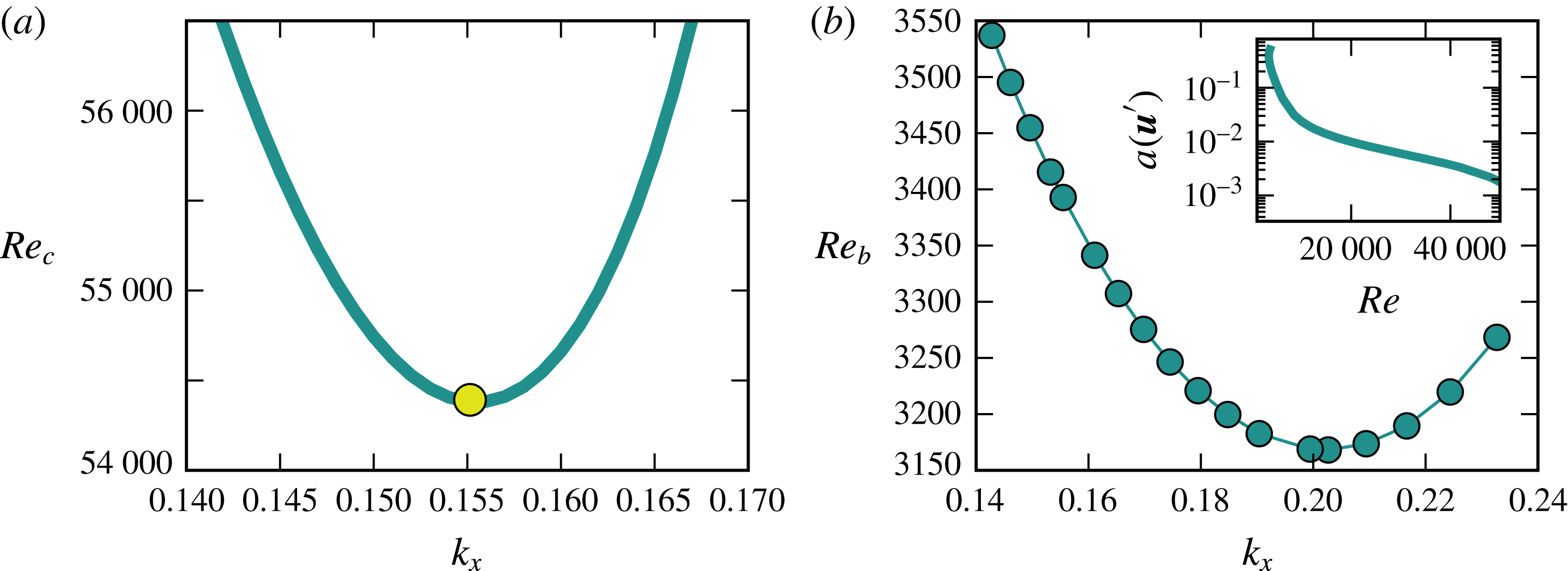
). The critical Reynolds numbers as a function of streamwise wavenumber agree with the results of Hocking (Reference Hocking1975) and the more recent ones of Fransson & Alfredsson (Reference Fransson and Alfredsson2003); they are shown in figure 2(a). The critical Reynolds number found here is 54 379, which is achieved for a streamwise wavenumber 0.1555. Wedin, Cherubini & Bottaro (Reference Wedin, Cherubini and Bottaro2015) showed recently that the instability of the flow moves to lower Reynolds numbers if the plate’s permeability is not neglected.
The Tollmien–Schlichting-like travelling wave solution which bifurcates subcritically from the laminar flow has been traced in
 $\mathit{Re}$
for various values of the streamwise wavenumber. A bifurcation diagram of the waves is included in figure 2(b) in an inset. For the ordinate of the diagram we use the amplitude,
 $$\begin{eqnarray}a(\boldsymbol{u}^{\prime })=\sqrt{\left(\frac{1}{L_{x}L_{z}}\int _{L_{x}}\int _{L_{y}}\int _{L_{z}}\boldsymbol{u}^{\prime 2}\,\text{d}x\,\text{d}y\,\text{d}z\right)},\end{eqnarray}$$
of the flow field, where
 $L_{x}$
and
 $L_{z}$
are the streamwise and spanwise wavelengths of the computational domain. The plot shows that close to the turning point the amplitude of the flow field increases dramatically. The dependence of the positions of the turning point on the wavenumber is given in figure 2(b). The minimal Reynolds number of the turning point is 3168, which is achieved for
 $k_{x}=0.203$
. These results show that as in the case of plane Poiseuille flow the two-dimensional waves connected to the instability of the base flow appear at Reynolds numbers much higher than the observed onset of subcritical turbulence, which was found to be at
 $Re\approx 270$
for ASBL (Khapko et al.
Reference Khapko, Schlatter, Duguet and Henningson2016).
The stability boundary of the laminar state of isothermal ASBL (
 $\mathit{Ra}=0$
) is shown in (a). The critical Reynolds number
 $Re_{c}=54\,379$
is marked by a circle. (b) Shows the Reynolds number
 $Re_{b}$
of the subcritical bifurcation point for the TS-wave versus streamwise wavenumber
 $k_{x}$
. The inset shows a bifurcation diagram of the TS-wave for
 $k_{x}=k_{c}$
which uses the amplitude of the flow field
 $a(\boldsymbol{u}^{\prime })$
on the vertical axis.

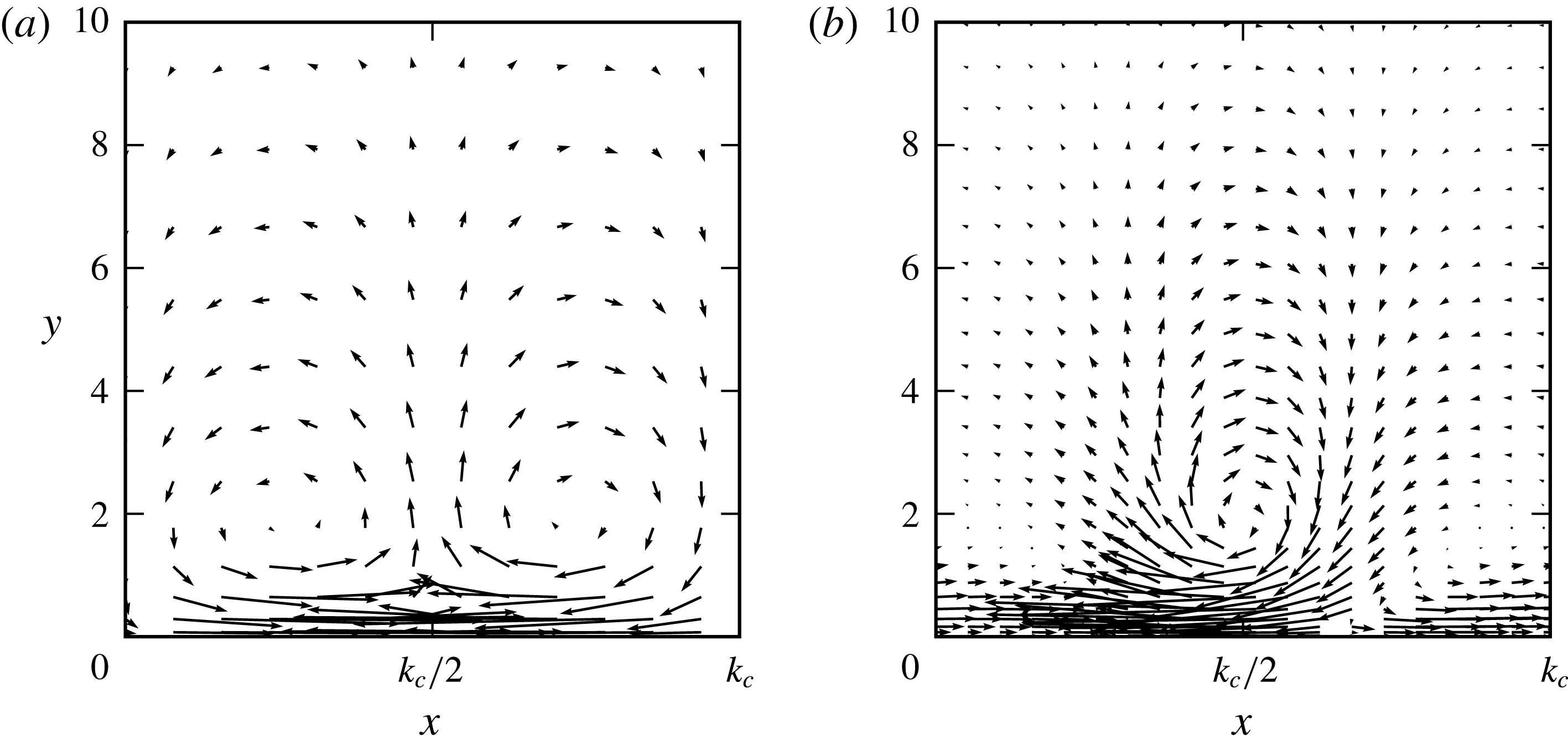
Visualizations of the bifurcating two-dimensional solutions are given in figure 3 for different Reynolds numbers. Because the flow has no discrete symmetry with respect to the wall-normal direction
 $y$
, the clockwise and counter-clockwise rolls behave differently with
 $\mathit{Re}$
. Close to the bifurcation point at
 $Re=50\,000$
(figure 3
a) the rolls are almost symmetric. When
 $Re$
is decreased the counter-clockwise roll becomes strongly deformed while the clockwise roll maintains its shape and becomes narrower only (figure 3
b).
Visualizations of the TS-wave bifurcating from the base flow for
 $Re=50\,000$
(a) and
 $Re=8475$
(b). In both cases the streamwise wavenumber is 0.1555. The direction of the flow is from left to right.

3.3 Stability analysis for
$\mathit{Re}=0$
and
$\mathit{Ra}\neq 0$


We now turn to the stability of the thermal boundary layer for the case
 $\mathit{Re}=0$
. The corresponding Orr–Sommerfeld equations (3.7)–(3.9) are solved using up to 600 Chebychev polynomials and truncation lengths
 $L_{y}$
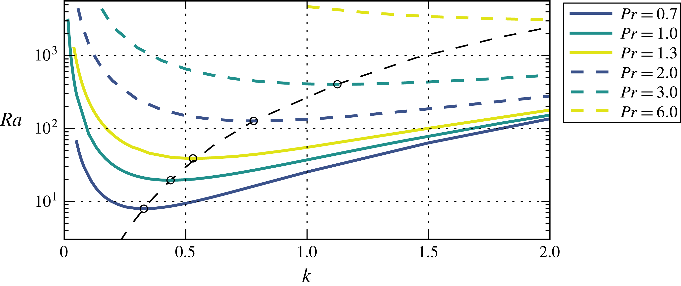
up to 250 (for small Prandtl numbers). In figure 4 the calculated stability curves for various Prandtl numbers, including the cases
 $\mathit{Pr}=0.7$
(air) and
 $\mathit{Pr}=6$
(water), are shown. The results show a strong dependence on the Prandtl number and therefore on the relative size of the thermal to the viscous boundary layer that is in contrast to the standard Rayleigh–Bénard convection. For the case
 $\mathit{Pr}=1$
a critical Rayleigh number of 19.4705 and a critical wavenumber of 0.438 are obtained. For lower values of
 $\mathit{Pr}$
the critical wavenumber and Rayleigh number move to lower values, while they move to higher ones if larger values of
 $\mathit{Pr}$
are considered.
Stability boundary for
 $\mathit{Re}=0$
and different values of the Prandtl number. For each Prandtl number the lowest critical Rayleigh number is marked by a black circle.

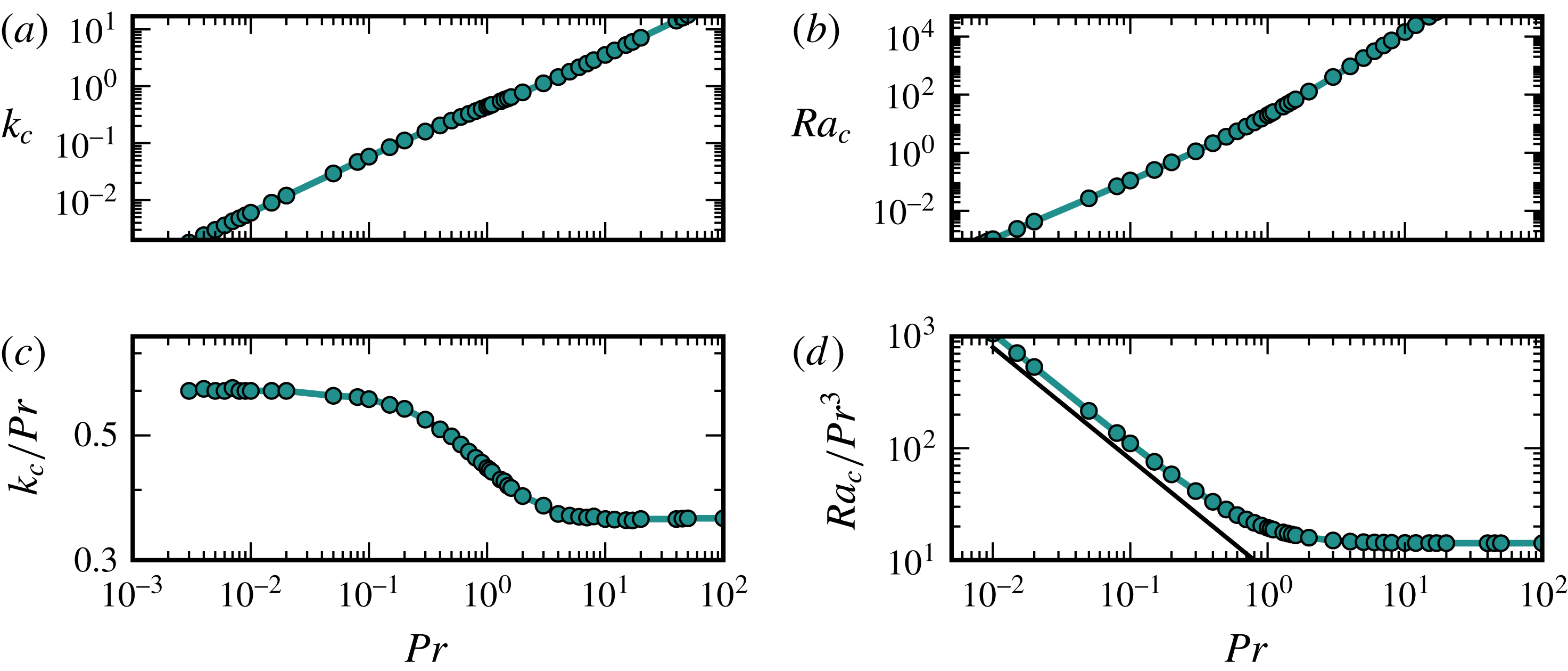
Prandtl number dependence of critical wavenumber and critical Rayleigh number as a function of Prandtl number are shown in (a,b), respectively. (c,d) Show the results after a change of the length scale to the thermal boundary layer thickness
 $\unicode[STIX]{x1D6FF}_{\unicode[STIX]{x1D703}}=\unicode[STIX]{x1D6FF}/\mathit{Pr}$
. The thin black line in (d) indicates a
 $\mathit{Pr}^{-1}$
scaling.

The critical Rayleigh and wavenumber are shown in figure 5(a,b) in dependence on the Prandtl number. The graphs show that the dependence of the critical wavenumber on
 $\mathit{Pr}$
is approximately linear. The
 $\mathit{Pr}$
-dependence of the critical Rayleigh number seems to follow a power law, with an exponent near two for
 $\mathit{Pr}<1$
and near three for
 $\mathit{Pr}>1$
.
An explanation for the
 $\mathit{Pr}$
-dependence of the critical Rayleigh number may be obtained from a discussion of the relevant scales, similar to the one given by Grossmann & Lohse (Reference Grossmann and Lohse2000b
) for normal Rayleigh–Bénard convection. The definition of
 $\mathit{Ra}$
uses the length scale of the velocity boundary layer
 $\unicode[STIX]{x1D6FF}$
and the full temperature difference. For large values of
 $\mathit{Pr}$
the thickness of the temperature boundary layer
 $\unicode[STIX]{x1D6FF}_{\unicode[STIX]{x1D703}}$
is much smaller than the one of the velocities. Therefore, the length scale relevant for the forces driving convection is
 $\unicode[STIX]{x1D6FF}_{\unicode[STIX]{x1D703}}$
. A Rayleigh number based on
 $\unicode[STIX]{x1D6FF}_{\unicode[STIX]{x1D703}}$
can be obtained by multiplication of
 $\mathit{Ra}$
with
 $1/\mathit{Pr}^{3}$
because
 $\mathit{Ra}\propto \unicode[STIX]{x1D6FF}^{3}$
and
 $\unicode[STIX]{x1D6FF}/\unicode[STIX]{x1D6FF}_{\unicode[STIX]{x1D703}}=\mathit{Pr}$
. By the same argument, the wavenumber based on
 $\unicode[STIX]{x1D6FF}_{\unicode[STIX]{x1D703}}$
is obtained from the one based on
 $\unicode[STIX]{x1D6FF}$
by dividing by
 $\mathit{Pr}$
. The results of this change in length scale are shown in figure 5(c,d). For the wavenumber as well as for
 $\mathit{Ra}$
the change of the length scale leads to critical values that for large values of
 $\mathit{Pr}$
become independent of the Prandtl number. The critical wavenumber
 $k_{\unicode[STIX]{x1D703},c}$
and Rayleigh number
 $\mathit{Ra}_{\unicode[STIX]{x1D703}}$
based on the thickness of the temperature boundary layer that are asymptotically reached for large Prandtl numbers are 0.363 and 14.3, respectively.
For the case
 $\mathit{Pr}<1$
, two modifications have to be taken into account. The observation that the rescaled critical wavenumber reaches a plateau value for small values of
 $\mathit{Pr}$
(see figure 5
c), suggest that the thickness of the thermal boundary layer determines the instability also for this parameter regime. However, since the viscous boundary layer is smaller than the thermal boundary layer, the temperature drops only by a fraction
 $(\unicode[STIX]{x1D6FF}/\unicode[STIX]{x1D6FF}_{\unicode[STIX]{x1D703}})T_{0}=\mathit{Pr}\,T_{0}$
, and it is this smaller range that should be taken for the temperature difference in the definition of the Rayleigh number. Accordingly, there is a factor of
 $\mathit{Pr}$
from the temperature difference, and a factor
 $\mathit{Pr}^{-3}$
from the scaling of the height, resulting in a scaling of
 $\mathit{Pr}^{2}$
for the critical Rayleigh number, or
 $\mathit{Pr}^{-1}$
in the scaling used in figure 5(d).
By using the Newton method (Viswanath Reference Viswanath2007) included in the channelflow package, it is possible to identify the exact solutions bifurcating at the linear instability and to continue them in Rayleigh number. The used resolution is
 $N_{x}\times N_{y}\times N_{z}=4\times 49\times 32$
. Four modes in the
 $x$
-direction are sufficient because the structures are two-dimensional and do not vary in
 $x$
-direction. In the wall-normal direction a truncation length
 $L_{y}$
is chosen which is large enough so that there is no noticeable influence on the structures by the wall. For lower branch states
 $L_{y}=40$
is sufficient, while for upper branch states values up to
 $L_{y}=110$
with a resolution
 $N_{y}=129$
are necessary.
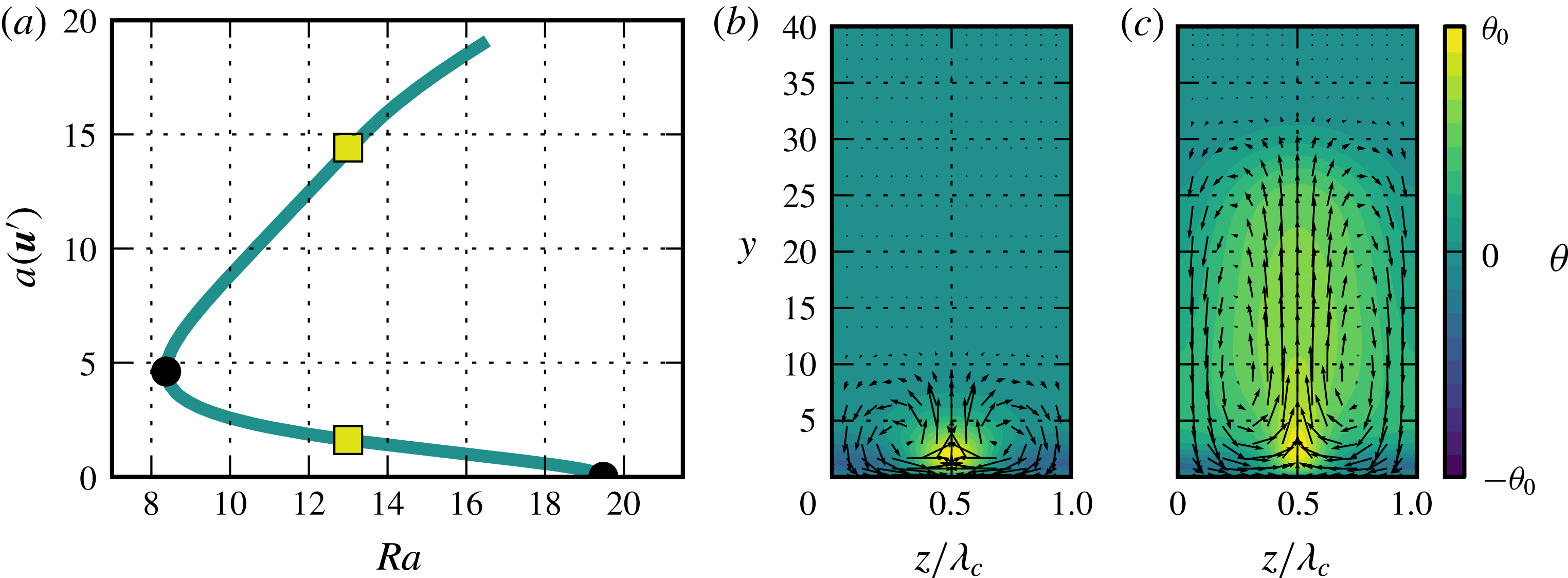
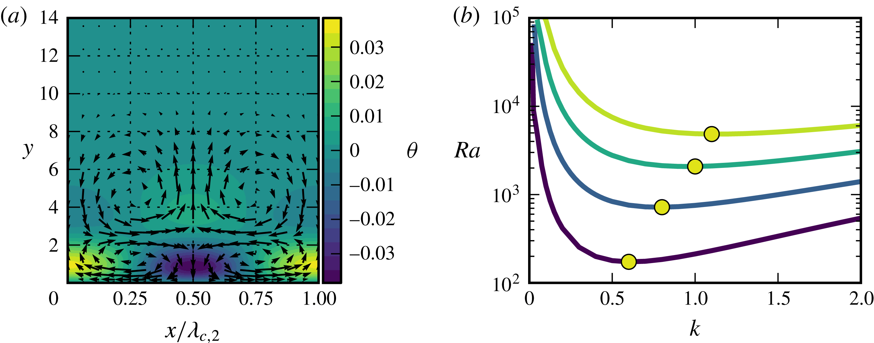
(a) Shows the bifurcation diagram of the secondary solution with
 $k=k_{c}=0.4305$
. On the
 $y$
-axis the amplitude
 $a(\boldsymbol{u}^{\prime })$
of the solution is used. (b,c) Show visualizations of the flow and temperature fields for the lower and the upper branches of
 $R_{1}$
. The positions of the visualization are marked in (a) using yellow squares. The velocity field is visualized by the arrows. The temperature field is represented by the colours. For the lower branch
 $\unicode[STIX]{x1D703}_{0}=0.19\,\mathit{Ra}$
and for the upper branch
 $\unicode[STIX]{x1D703}_{0}=0.32\,\mathit{Ra}$
.

The bifurcating ECS identified by the Newton method is an equilibrium solution which we refer to as roll state
 $R_{1}$
in the following. A bifurcation diagram of the ECS for the critical wavenumber
 $k_{c}$
and
 $\mathit{Pr}=1$
is given in figure 6(a). The diagram shows that in contrast to the case of Rayleigh–Bénard flow the bifurcation is subcritical. For the critical wavenumber
 $k_{c}=0.4304$
used for the bifurcation diagram, the turning point of the solutions lies at
 $\mathit{Ra}=8.374$
but this value varies with wavenumber. With decreasing wavenumber the turning point moves to lower values of
 $\mathit{Ra}$
while with increasing wavenumber it moves to higher Rayleigh numbers.
The flow and temperature fields for the lower and the upper branch of the state shown in figure 6(b,c) reveal that the secondary solution
 $R_{1}$
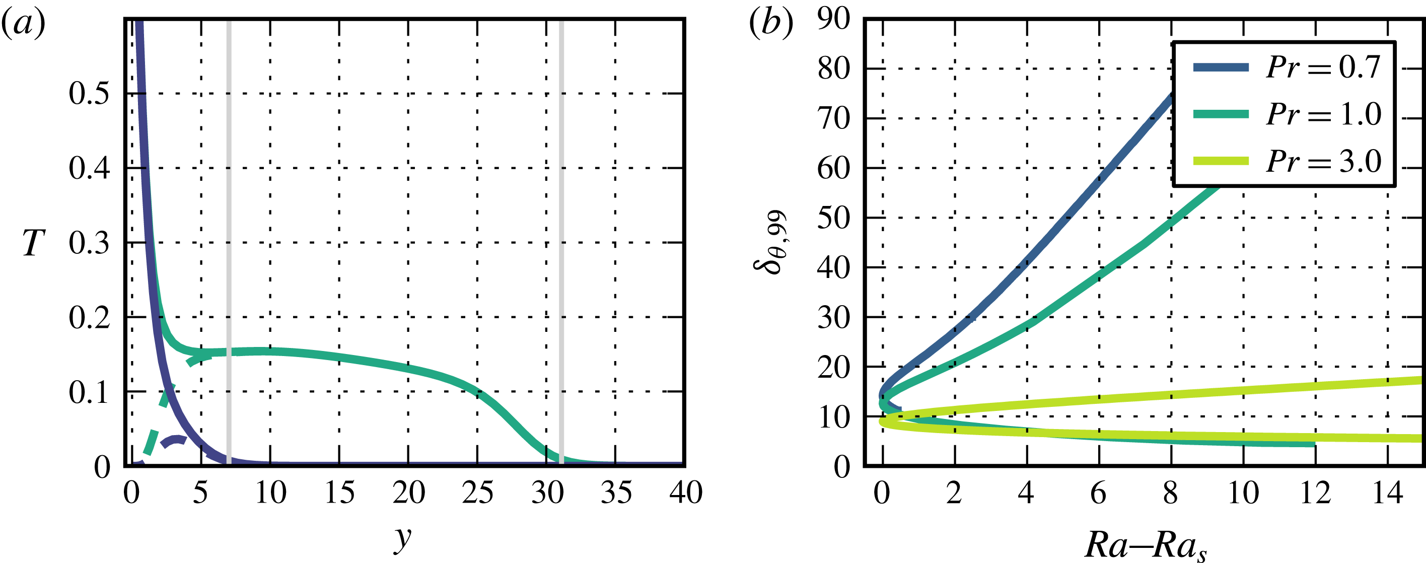
consists of counter-rotating convection rolls. With increasing distance from the bifurcation point rolls grow in height while maintaining their width, so that their aspect ratio (height/width) increases. To quantify the growth in height we use the thickness
 $\unicode[STIX]{x1D6FF}_{\unicode[STIX]{x1D703},99}$
, defined as the distance to the plate at which the mean temperature profile reaches
 $0.01T_{0}$
for the first time. The definition of
 $\unicode[STIX]{x1D6FF}_{\unicode[STIX]{x1D703},99}$
is illustrated in figure 7(a) using temperature profiles of both branches of
 $R_{1}$
. The variation of the quantity
 $\unicode[STIX]{x1D6FF}_{\unicode[STIX]{x1D703},99}$
with
 $\mathit{Ra}$
for different Prandtl numbers for the lower and the upper branches of the roll solution is shown in figure 7(b). While for the lower branch of
 $R_{1}$
the height varies only slightly with
 $\mathit{Ra}$
, the extension of the upper branch increases monotonically with the Rayleigh number. The rate of increase with
 $\mathit{Ra}$
as well as the absolute values of the height depend strongly on the Prandtl number. For small values of
 $\mathit{Pr}$
they are larger than for higher values of
 $\mathit{Pr}$
. Specifically, the increase of the height of the upper branch solution with Rayleigh number follows a linear law (for sufficient distance from the turning point). The slope increases with decreasing Prandtl number from approximately 0.4 for
 $\mathit{Pr}=3$
to 8.1 for
 $\mathit{Pr}=0.7$
. The results show that for small Prandtl number the roll solutions extend remarkably far above the plate, and their reach seems to increase with
 $\mathit{Ra}$
, independent of
 $\mathit{Pr}$
.
(a) Temperature profiles of the lower (blue) branch and upper branch (cyan) of the secondary solution
 $R_{1}$
at
 $\mathit{Ra}=13$
versus distance
 $y$
above the plate. For the total temperature profile a solid line is used and the deviations from the base profile are shown by dashed lines. The positions of
 $\unicode[STIX]{x1D6FF}_{\unicode[STIX]{x1D703},99}$
are marked using grey lines. (b) Values of
 $\unicode[STIX]{x1D6FF}_{\unicode[STIX]{x1D703},99}$
of the secondary solution
 $R_{1}$
in dependence on the distance to the saddle-node point for different Prandtl numbers. For each Prandtl number the wavelength of the state shown is chosen to be the critical wavelength at the particular value of the Prandtl number.

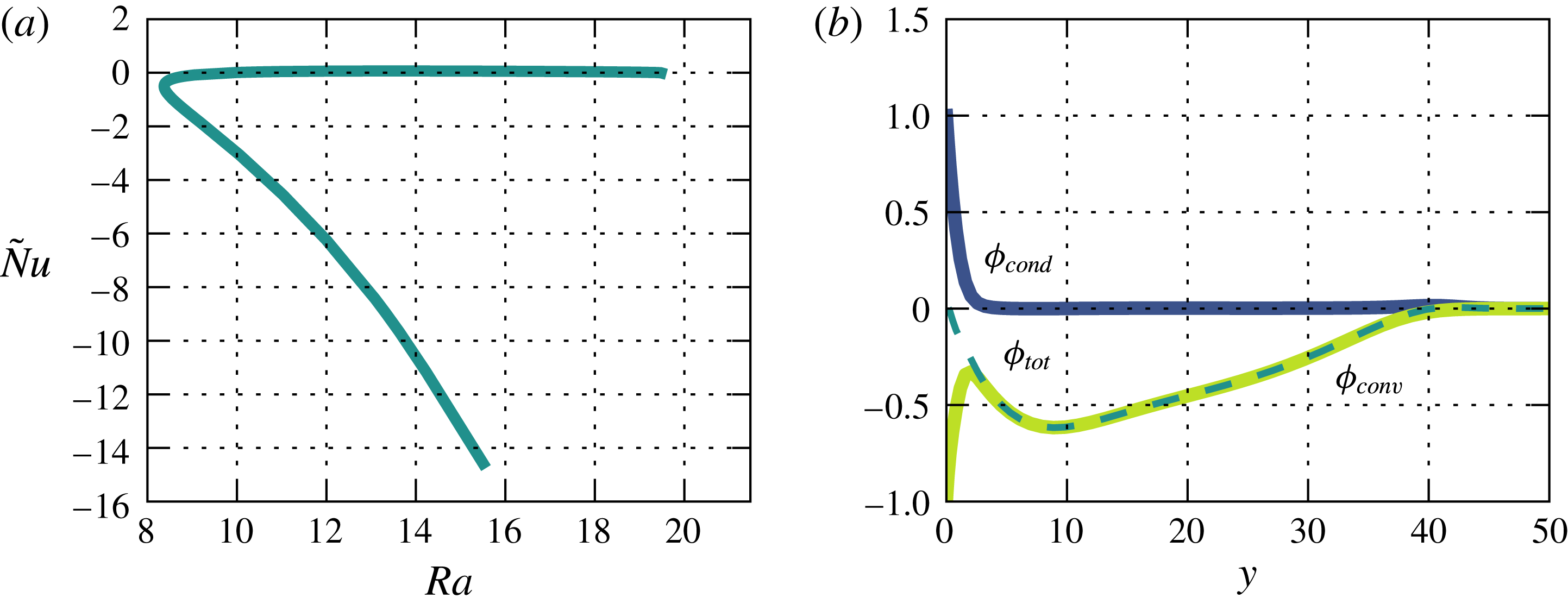
The secondary roll solutions have different heat transport properties than the base flow. In figure 8(a) the Nusselt number
 $\tilde{\mathit{Nu}}$
is shown as a function of Rayleigh number for the roll solution
 $R_{1}$
with
 $k=k_{c}$
and
 $\mathit{Pr}=1$
. To rationalize the negative values of
 $\tilde{\mathit{Nu}}$
the contributions of the convective and the conductive heat transport for a state on the upper branch of
 $R_{1}$
are shown as a function of
 $y$
in figure 8(b). Especially for the upper branch, the heat transport due to convection has large negative values, leading to negative values of the integrated quantity
 $\tilde{\mathit{Nu}}$
with large modulus. The figure shows that for the secondary solution
 $R_{1}$
the conductive heat transport is only relevant close to the wall and quickly drops to zero for larger values of
 $y$
. Furthermore, the plot illustrates that indeed the convective heat transport causes the large negative values of
 $\tilde{\mathit{Nu}}$
(the integral over the dashed curve). If only the deviations from the base flow are considered, the up-flow and down-flow regions in the roll state
 $R_{1}$
are approximately of equal strength (see figure 6
b,c) and the temperatures in both regions are comparable as well. Since the base flow has a negative wall-normal component, the symmetry is broken and the negative contribution to the convective heat flux due to the down-flow region becomes larger than the positive contribution of the up-flow region. Thus, the average convective heat flux is negative for
 $R_{1}$
. However, there are also turbulent states or coherent states with high asymmetry for which positive values of
 $\tilde{\mathit{Nu}}$
are obtained.
Nusselt number
 $\tilde{Nu}$
as a function of the Rayleigh number for the secondary solution
 $R_{1}$
with
 $k=k_{c}$
at
 $Re=0$
is shown in (a). In (b) the contributions of the conductive (blue) and convective (yellow) heat flux are shown as functions of the wall-normal coordinate
 $y$
for the upper branch of
 $R_{1}$
at
 $\mathit{Ra}=15.5$
. The resulting total heat flux is shown by the dashed cyan line. The quantities are normalized with respect to the Rayleigh number.

For high Rayleigh numbers another two-dimensional eigenmode becomes unstable. For
 $\mathit{Pr}=1$
, the critical wavenumber for this mode is 0.612 and the critical Rayleigh number is 173. This bifurcation is subcritical, and gives rise to an equilibrium solution henceforth referred to as
 $R_{2}$
. The state
 $R_{2}$
has a set of four rolls staggered on top of each other, with the top pair similar to
 $R_{1}$
and the bottom one rather flat, as shown in figure 9(b). The second pair of rolls of the
 $R_{2}$
solution has its centre at a distance of approximately 5 from the plate where the temperature gradient is already quite low. This is reminiscent of the free-stream coherent structures of isothermal ASBL described by Deguchi & Hall (Reference Deguchi and Hall2014) and Kreilos et al. (Reference Kreilos, Gibson and Schneider2016), which have vortices at a distance to the plate where the shear gradient is low.
In (a) a visualization of the exact solution
 $R_{2}$
that bifurcates from the second two-dimensional instability is shown. The wavenumber is 0.612 and the Rayleigh number is 167. (b) Shows stability curves for the second to fifth two-dimensional unstable modes for
 $\mathit{Pr}=1$
. The critical Rayleigh numbers are marked with a yellow circle.

For even higher Rayleigh numbers further modes become unstable. Each additional unstable mode has one more layer of rolls. The stability curves for the second to fifth two-dimensional unstable modes are shown in figure 9(b). The critical Rayleigh numbers for the third, fourth and fifth unstable mode are 719.2, 2082 and 4846, respectively. The corresponding critical wavenumbers are 0.78, 1.0 and 1.1. Since they are very unstable, the ECS created in these bifurcation are of minor importance for the dynamics and thus not treated in this paper.
3.4 Stability analysis for
$\mathit{Re}\neq 0$
and
$\mathit{Ra}\neq 0$


The stability of the base flow for the case that shear and buoyancy are present can take advantage of the fact that a generalization of Squire’s theorem holds for this flow (Gage & Reid Reference Gage and Reid1968), so that it suffices to know the stability boundary for transversal and longitudinal modes to obtain a complete stability diagram.
A stability analysis of modes that depend only on the spanwise wavenumber and are invariant in the streamwise direction (longitudinal modes) yields, for any Prandtl number, the same critical Rayleigh numbers as in the case of vanishing Reynolds number.
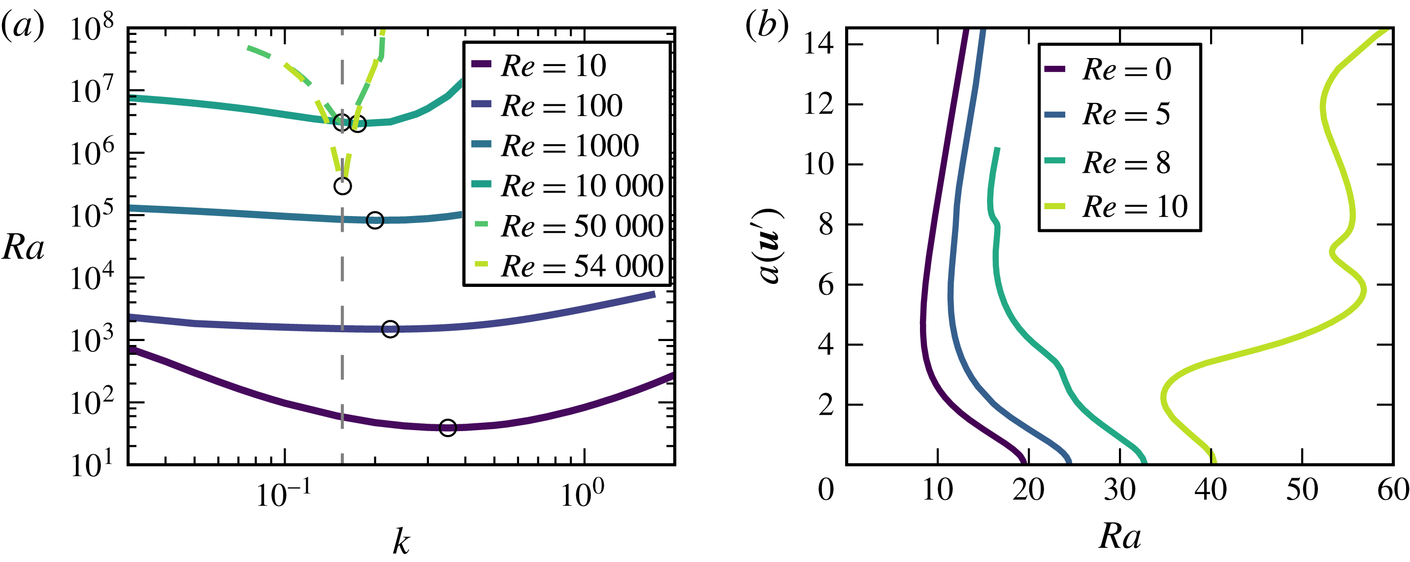
Initially, for spanwise invariant modes (transversal modes) an increase of the Reynolds number has a stabilizing effect. Figure 10(a) shows stability curves of the most unstable transversal mode for various Reynolds numbers. Up to a Reynolds number of approximately 35 000 an increase of
 $\mathit{Re}$
results in larger critical Rayleigh number. If the Reynolds number is further increased the transversal modes are rapidly destabilized again until at
 $Re_{c}=54\,379$
they are unstable for
 $\mathit{Ra}=0$
. The critical wavenumbers move monotonically towards the critical wavenumber for the isothermal case with increasing Reynolds number.
We track the travelling wave solutions which bifurcate from the base flow when the transversal mode becomes unstable for various Reynolds numbers. The bifurcation diagrams of the transversal waves with
 $k=k_{c}=0.4304$
in figure 10(b) show that for finite values of
 $Re$
the bifurcation is still subcritical in the Rayleigh number, but the turning point of the solution branch moves to higher values of
 $\mathit{Ra}$
.
(a) Shows stability curves of the most unstable transversal mode in dependence on the Reynolds number. For each Reynolds number a black circle marks the critical Rayleigh number. The critical wavenumber of isothermal ASBL is marked by a dashed grey line. In (b) bifurcation diagrams of the two-dimensional transversal waves bifurcating from the laminar flow are shown for various Reynolds numbers.

For systems that are thermally stratified and under the influence of shear an often used dimensionless number is the Richardson number,
 $$\begin{eqnarray}\mathit{Ri}=\frac{g\unicode[STIX]{x1D6FD}T_{0}\unicode[STIX]{x1D6FF}}{U_{\infty }^{2}}=\frac{\mathit{Ra}}{\mathit{Re}^{2}\mathit{Pr}},\end{eqnarray}$$
which relates the buoyancy to the flow gradient. The value of
 $\mathit{Ri}$
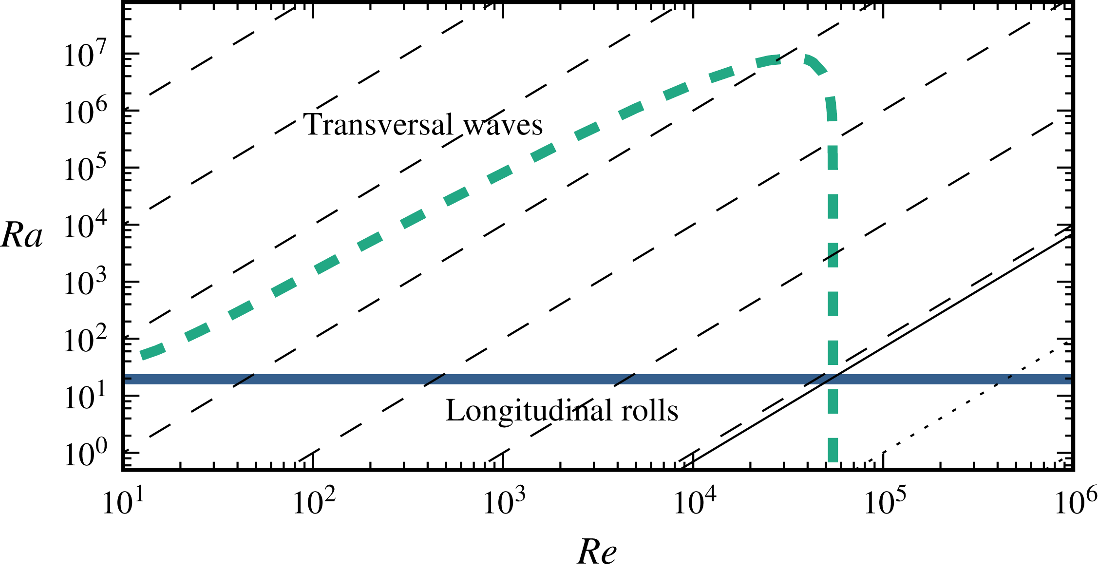
is a measure for the importance of natural convection compared to forced convection. As in the study of Gage & Reid (Reference Gage and Reid1968) for Rayleigh–Bénard–Poiseuille flow it is possible to give a critical value of the Richardson number which marks the transition between natural and forced convection. For ASBL over a heated plate we obtain a critical Richardson number of approximately
 $\mathit{Ri}_{c}=19.47/(54379^{2}\times 1.0)\approx 7\times 10^{-9}$
. For smaller Richardson numbers the system has an instability to transversal rolls or waves while for larger values of
 $\mathit{Ri}$
the system has an instability to longitudinal rolls. The resulting complete stability diagram for the flow (for
 $\mathit{Pr}=1$
) with the critical Rayleigh numbers of transversal and longitudinal modes for different
 $\mathit{Re}$
and lines of constant Richardson number, is shown in figure 11.
Stability diagram of TASBL in dependence on
 $\mathit{Ra}$
and
 $\mathit{Re}$
. Critical Rayleigh numbers for longitudinal rolls and transversal waves are shown using solid blue and dashed cyan lines. The solid black line corresponds to the critical Richardson number
 $\mathit{Ri}_{c}=7\times 10^{-9}$
. where the instability switches from longitudinal rolls to transversal waves. Lines of constant Richardson number are shown using dashed and dotted lines for
 $\mathit{Ri}<\mathit{Ri}_{c}$
and
 $\mathit{Ri}>\mathit{Ri}_{c}$
, respectively. The values of the Richardson numbers decrease by factors of
 $10^{2}$
starting with
 $10^{4}$
in the upper left corner.

4 Two-dimensional solutions and subcritical transient chaos
In this section we analyse the stability of the two-dimensional secondary solutions and describe the bifurcating states. The analysis is restricted to the secondary states with a wavenumber equal to the critical one and to two-dimensional superharmonic disturbances with wavenumbers that are integer multiples of the ones of the secondary solution. The stability analysis of the solutions is performed using an Arnoldi method included in the Channelflow package and adapted to work with an additional temperature field. The calculations use a computational domain with
 $L_{x}=0.1$
,
 $L_{z}=\unicode[STIX]{x1D706}_{0}$
and
 $L_{y}=40$
and a resolution of
 $N_{x}\times N_{y}\times N_{z}=4\times 65\times 32$
, which is a good approximation of the two-dimensional system.
The stability analysis shows that the lower branch of the secondary solution
 $R_{1}$
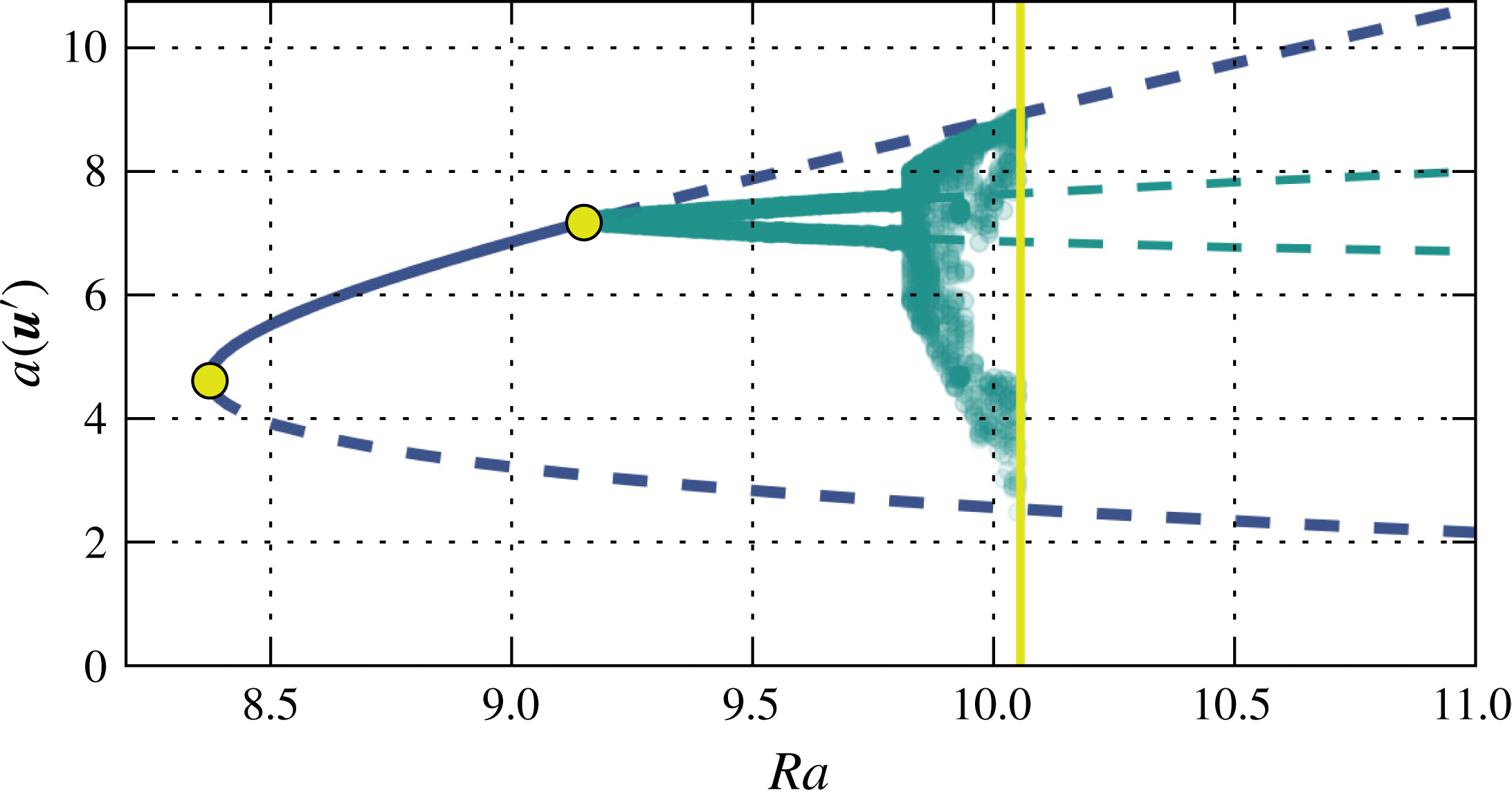
has one unstable direction. Thus, it is an edge state (Skufca, Yorke & Eckhardt Reference Skufca, Yorke and Eckhardt2006; Schneider, Eckhardt & Yorke Reference Schneider, Eckhardt and Yorke2007) for the two-dimensional system because its stable manifold can separate two regions of the state space. Right after the turning point the upper branch of the solution is stable. When the Rayleigh number is increased, a pair of complex conjugate eigenvalues becomes unstable at
 $\mathit{Ra}\approx 9.15$
, indicating a Hopf bifurcation. This bifurcation creates a stable periodic orbit which we refer to as
 $PO_{1}$
in the following. A supplementary movie illustrating the dynamics of the orbit is available online at http://dx.doi.org/10.1017/jfm.2016.514 (movie 1).
Bifurcation diagram of
 $R_{1}$
with wavenumber
 $k=k_{c}$
at
 $\mathit{Pr}=1$
and
 $\mathit{Re}=0$
. The curve for
 $R_{1}$
is shown as a blue line. Chaotic and periodic states are indicated by cyan points representing minima and maxima of
 $a(\boldsymbol{u}^{\prime })$
in the course of time. In addition the dashed cyan lines show the minimum and maximum of
 $a(\boldsymbol{u}^{\prime })$
for the orbit
 $PO_{1}$
. The bifurcation points of
 $R_{1}$
and
 $PO_{1}$
are marked by yellow circles. The solid yellow line marks the position of the boundary crisis bifurcation near
 $\mathit{Ra}=10.0$
which destroys the attractor.

If the Rayleigh number is further increased, the periodic orbit undergoes a Neimark–Sacker bifurcation (Kuznetsov Reference Kuznetsov1998) which creates a stable torus. Further bifurcations then create a chaotic attractor. A supplementary movie illustrating the dynamics of a trajectory on the chaotic attractor is available online (movie 2). The bifurcation diagram, sampled by plotting maxima of
 $a(\boldsymbol{u}^{\prime })$
for trajectories on the attractor, is shown in figure 12. Eventually, the chaotic attractor is converted into a chaotic saddle by a boundary crisis bifurcation (e.g. Lai & Tél Reference Lai and Tél2011). For
 $k=k_{c}$
this happens at
 $\mathit{Ra}\approx 10.06$
. Following the boundary crisis, for
 $\mathit{Ra}<\mathit{Ra}_{c}$
initial conditions can be found which transiently show chaotic dynamics before they finally return to the base flow (supplementary movie 3 online). The bifurcation cascade that eventually creates transient chaos in this open flow is akin to those that were found to exist in internal flows such as plane Couette flow (Kreilos & Eckhardt Reference Kreilos and Eckhardt2012), pipe flow (Avila et al.
Reference Avila, Mellibovsky, Roland and Hof2013) or plane Poiseuille flow (Zammert & Eckhardt Reference Zammert and Eckhardt2015). An important difference is that in the present case the exact solution which is the starting point of the cascade originates from a bifurcation of the base flow.
5 Three-dimensional states and localization
Up to this point we have considered two-dimensional exact coherent states, with a modulation in spanwise or streamwise and normal direction. Here, we turn to three-dimensional states, in particular states that are either extended or localized in both spanwise and streamwise direction. For all solutions in this section the Prandtl number is fixed at
 $\mathit{Pr}=1$
and there is no flow, the Reynolds number is
 $\mathit{Re}=0$
.
5.1 Straight rolls, squares and hexagons
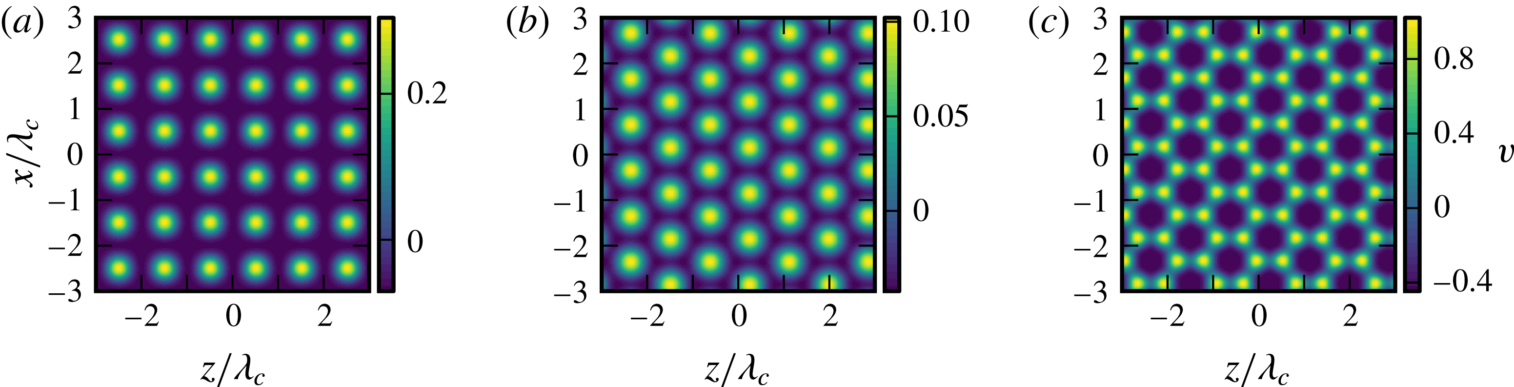
Using a Newton method we can identify different secondary solutions of the three-dimensional system which bifurcate from the base profile at the critical Rayleigh number. The simplest solutions which also exist in the two-dimensional case are straight rolls which are translationally invariant along an axis parallel to the plates. In addition to the straight rolls, a secondary solution exists which shows a square pattern of up-flow regions. This solution has equal wavenumbers in both directions parallel to the plate, as shown in figure 13(a). The visualization shows the wall-normal velocity in a plane parallel to the plate in a distance of 1.5. A continuation of this ECS in Rayleigh number shows that the turning point is at slightly lower Rayleigh numbers than for the two-dimensional roll solution
 $R_{1}$
. The upper branch of this three-dimensional state again reaches remarkably far above the plates.
It is also possible to identify two different kinds of secondary solutions with hexagonal pattern. They are formed by superpositions of three solutions with wave vectors rotated by
 $2\unicode[STIX]{x03C0}/3$
. One of the hexagonal patterns has a up-flow region in the centre of each hexagon while for the other one the centre contains the down-flow region. Following the nomenclature of Rayleigh–Bénard convection (Getling Reference Getling1998) they can be named
 $l$
- and
 $g$
-cells. Visualization of both types of hexagons are shown in figure 13(b,c).
Visualization of the three-dimensional secondary solutions at
 $\mathit{Ra}=17$
. (a) Shows the square solution and (b,c) the hexagonal solutions of
 $l$
- and
 $g$
-type, respectively. For all panels the wall-normal velocity (deviation from laminar profile) is shown in a plane parallel to the plate at
 $y\approx 1.5$
.

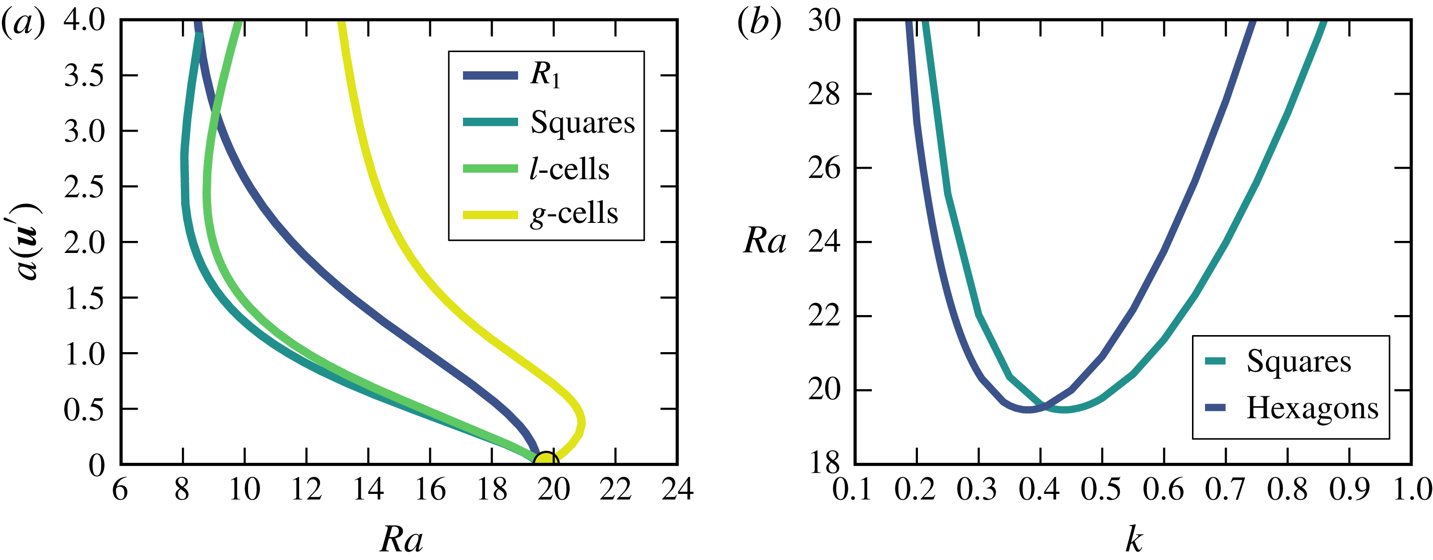
The bifurcation curves for a wavelength equal to the critical one of the square pattern are shown in figure 14. The figure shows that the bifurcation for the
 $g$
-hexagons is initially supercritical and turns to lower
 $\mathit{Ra}$
only with increasing amplitude, while
 $l$
-hexagons bifurcate subcritically right from the base flow. The lowest values in
 $\mathit{Ra}$
are achieved for
 $l$
-hexagons.
(a) Shows a bifurcation diagram of the four equilibrium patterns that exist in the three-dimensional system for
 $\mathit{Re}=0$
. For each solution the wavenumber is
 $k=k_{c}=0.4305$
. In (b) the stability lines for the hexagonal and the square instability are compared.

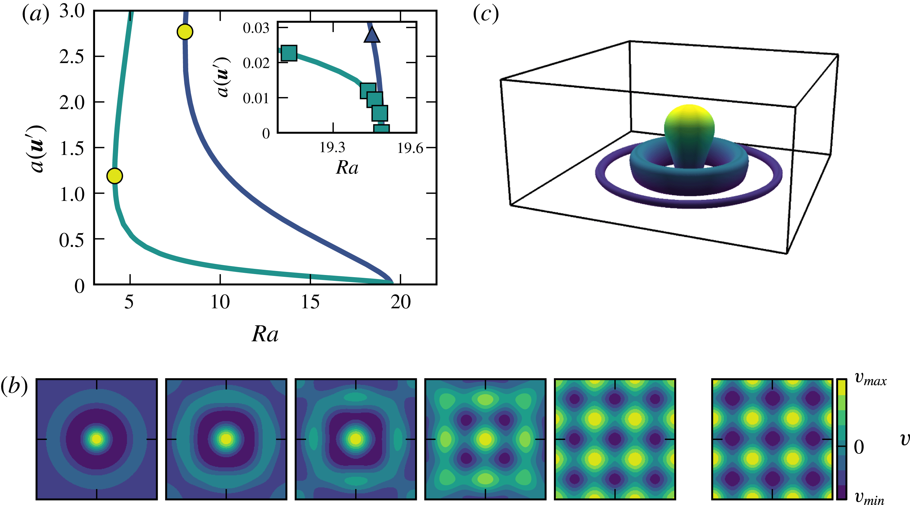
(a) Shows the bifurcation diagram for the doubly localized equilibrium solution
 $C_{1}$
(cyan) and the spatially extended equilibrium (blue). The inset shows the bifurcation diagram close to the point where
 $C_{1}$
connects to the spatially extended pattern. In (b) the states which are marked with the squares in the inset of (a) are visualized. The plots show the wall-normal velocity
 $v$
in a plane parallel to the plate in a distance of 1.5. The leftmost picture corresponds to the square at the lowest Rayleigh number. The rightmost panel in (b) shows the wall-normal velocity
 $v$
for the state marked in (a) by the triangle. In (c) the iso-surface
 $v=0.0005$
(deviation from laminar) is shown for the doubly localized equilibrium
 $C_{1}$
at
 $\mathit{Ra}=17.0$
,
 $\mathit{Re}=0$
and
 $\mathit{Pr}=1$
. The iso-surface is coloured according to the distance to the plate from blue to yellow.

For a given wavenumber the critical Rayleigh numbers for the square pattern and the hexagonal pattern differ slightly. The difference is too small to be noticeable in figure 14(a). In figure 14(b) the dependence of critical Rayleigh number on the wavenumber is shown for both patterns. In the presence of shear both the hexagonal and the square pattern instabilities move to higher Rayleigh numbers and the two-dimensional longitudinal rolls are the first instabilities to appear.
5.2 Localized states
With increasing distance to their bifurcation points the different secondary solutions undergo several three-dimensional instabilities. An interesting bifurcation of the square solution, which can be found in a domain with
 $L_{x}=L_{z}=6\unicode[STIX]{x1D706}_{c}$
and
 $L_{y}=40$
(resolution
 $N_{x}\times N_{y}\times N_{z}=192\times 49\times 192$
), is located slightly below
 $\mathit{Ra}_{c}$
. The bifurcation is connected with a long-wavelength instability (Chantry, Willis & Kerswell Reference Chantry, Willis and Kerswell2014; Melnikov, Kreilos & Eckhardt Reference Melnikov, Kreilos and Eckhardt2014) in two directions and creates a three-dimensional solution which for lower Rayleigh numbers becomes spatially localized in both directions parallel to the plate. The bifurcation diagram in figure 15(a) shows the spatially extended square pattern together with the bifurcating solution. For the Rayleigh numbers marked in the bifurcation diagram flow visualizations of the solutions are given in figure 15(b). The visualizations illustrate how the spatially extended pattern turns into localized states. Slightly below the bifurcation point, the flow pattern looks like the one of the spatially extended state with an additional modulation. With decreasing Rayleigh number this modulation quickly becomes larger until a localized and rotational symmetric state is reached.
The three-dimensional visualization of the state at
 $\mathit{Ra}=17$
which is shown in figure 15(c) impressively illustrates the localization and the symmetry of the state. For localized convection states akin to the identified ECS but only localized in one spatial direction the term convecton has been introduced (e.g. Blanchflower Reference Blanchflower1999; Lo Jacono, Bergeon & Knobloch Reference Lo Jacono, Bergeon and Knobloch2011; Beaume et al.
Reference Beaume, Bergeon, Kao and Knobloch2013). Adopting this notation, we will call the doubly localized equilibrium a convecton and use the abbreviation
 $C_{1}$
.
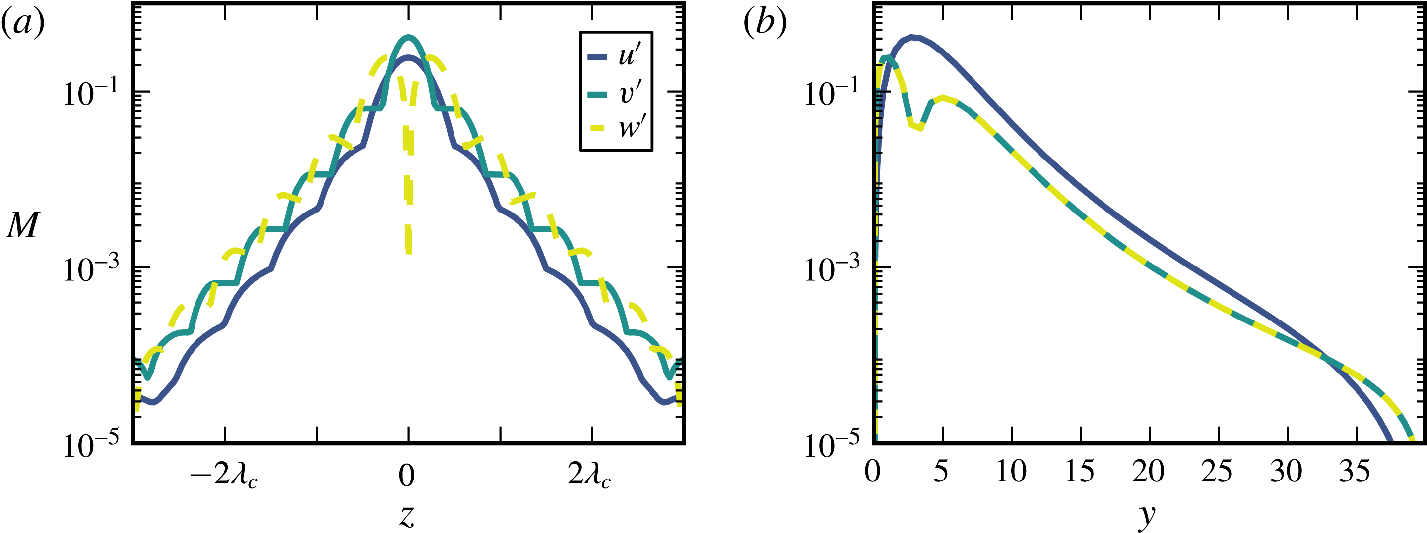
As a measure for the localization of the state
 $C_{1}$
we use the maximum norm,
 $$\begin{eqnarray}M(u^{\prime })=\max _{y,x}|u(x,y,z)^{\prime }|,\end{eqnarray}$$
here given for the streamwise component
 $u$
and in dependence of the spanwise coordinate. In figure 16 the maximum norm of all velocity components in the wall-parallel (a) and wall-normal (b) directions are shown. Since the localization is quite strong, the state exists also in larger domains and is not an artefact of the boundary conditions. In the directions parallel to the plate and also in wall-normal direction, the decay of the velocities is in good agreement with an exponential decay. In contrast to the doubly localized exact solution found in plane Poiseuille flow (Zammert & Eckhardt Reference Zammert and Eckhardt2014b
), the decay does not become algebraic for large distances. The difference can be rationalized by the fact that in plane Poiseuille flow the shear creates a large-scale flow around the exact solution which decays algebraically. Since in the present case the Reynolds number is zero, there is no shear and no large-scale flow. Thus, the decay is exponential over a large range.
Maximal values
 $M$
of the streamwise (blue), spanwise (yellow) and wall-normal (cyan) velocity component for the localized equilibrium at
 $\mathit{Ra}=17$
. (a) Shows the dependence on the wall-parallel coordinate
 $z$
and (b) the dependence on the wall-normal coordinate
 $y$
.

The turning point for
 $C_{1}$
lies at
 $\mathit{Ra}\approx 4.14$
. Close to the turning point, the localization becomes weaker again and especially the upper branch becomes very wide and very difficult to track numerically.
In addition to the localized equilibrium
 $C_{1}$
, many other localized states can be found. Starting with the spatially extended secondary solutions, we use two-dimensional window functions (Brand & Gibson Reference Brand and Gibson2014; Gibson & Brand Reference Gibson and Brand2014) to create initial guesses for Newton searches for localized equilibrium solutions. A two-dimensional window function
 $W(x,z)$
can be written as a product of two one-dimensional window functions. We use two different types of one-dimensional window functions, a Gaussian
 $$\begin{eqnarray}W_{1}(x)=A\exp (-Bx^{2})\end{eqnarray}$$
and the function
 $$\begin{eqnarray}W_{2}(x)=\frac{1}{4}\left(1+\tanh \left(\frac{6(A-x)}{B}+3\right)\right)\left(1+\tanh \left(\frac{6(A+x)}{B}+3\right)\right)\end{eqnarray}$$
introduced by Gibson & Brand (Reference Gibson and Brand2014). For appropriately chosen parameters
 $A$
and
 $B$
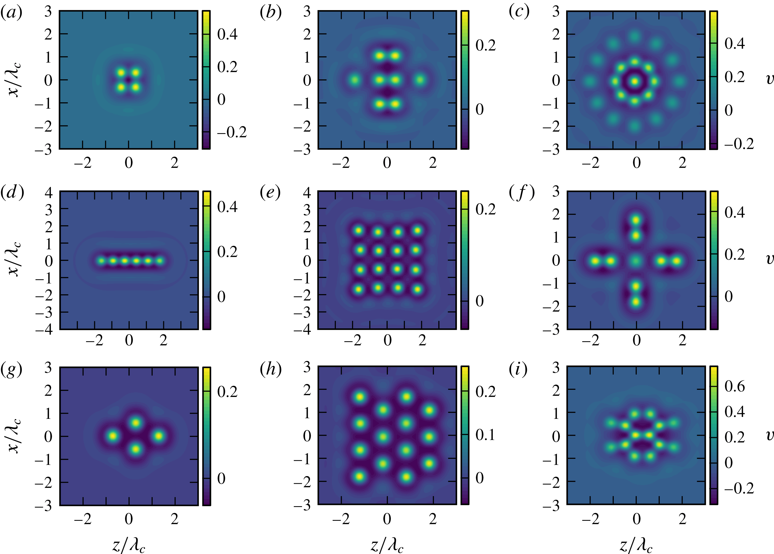
the obtained initial conditions are good initial guesses for equilibrium solutions. In figure 17 visualizations of different localized equilibrium solutions that were found for
 $\mathit{Ra}=17.8$
and
 $Pr=1$
are shown. The states shown in (a–c) were obtained from initial conditions created using the window function
 $W_{1}$
and for the state in (d,e) the window function
 $W_{2}$
was used. The equilibrium shown in (f) was obtained from an initial guess that was constructed by combining flow fields of several
 $C_{1}$
solutions. The states shown in (g–i) are obtained by applying window functions to the hexagonal patterns.
Different doubly localized solutions at
 $\mathit{Ra}=17.8$
. The Prandtl number is 1 and the Reynolds number is 0. The pictures show the wall-normal velocity in a plane parallel to the lower plate at
 $y\approx 1.5$
.

6 Summary and outlook
The present study extends the family of sheared convection problems from planar sheared convection (Clever & Busse Reference Clever and Busse1992) and Poiseuille–Rayleigh–Bénard flow (Nicolas Reference Nicolas2002) to the case of the ASBL, as a step towards analysing developing boundary layers. In all flows the transition is connected with roll states that are preferentially aligned with the flow direction, at least for Reynolds numbers close to the threshold. For higher Reynolds numbers, transverse rolls are preferred. The critical Rayleigh number shows a strong dependence on Prandtl number, which can be rationalized by relating it to an effective Rayleigh number that takes the temperature difference across the velocity field and the thickness of the thermal boundary layer into account.
The presence of a subcritical instability gives rise to a wide variety of secondary states, in particular of localized solutions of various shapes. While some of these states are reminiscent of plumes and other structures observed in thermal boundary layers, further studies of their dynamical properties will be required in order to establish this link more formally. It will be also be interesting to see how a spatial development as in Blasius boundary layers will influence the structures and their properties. Eventually, the study of the stability of convection combined with suitable boundary layer flows should provide a more reliable description of the transition from laminar to turbulent boundary layers and thus of the transition to the ultimate regime in thermal convection, (Grossmann & Lohse Reference Grossmann and Lohse2002).
Finally, it is intriguing that the upper branches of the coherent structures reach far into the free-stream region above the boundary layers. Certain ECS in shear boundary layers show similar properties (Deguchi & Hall Reference Deguchi and Hall2014; Kreilos et al. Reference Kreilos, Gibson and Schneider2016). The observation that the turbulent ASBL has remarkably thick boundary layers (Schlatter & Örlü Reference Schlatter and Örlü2011; Bobke, Örlü & Schlatter Reference Bobke, Örlü and Schlatter2016) thus suggesting that a study of the thermally heated ASBL in conjunction with investigations of the various exact coherent structures could also shed light on the large scale properties and organization of the flow beyond the transitional regime discussed here.
Acknowledgements
We thank J. F. Gibson for providing and maintaining channelflow. This work was supported in parts by the Deutsche Forschungsgemeinschaft (DFG) within FOR 1182 and by Stichting voor Fundamenteel Onderzoek der Materie (FOM) within the program ‘Towards ultimate turbulence’.
Supplementary movies
Supplementary movies are available at http://dx.doi.org/10.1017/jfm.2016.514.
Appendix A. Direct numerical simulation
For the study of ASBL with heated plate the Channelflow code (Gibson Reference Gibson2012) was adapted to integrate the set of coupled equations (2.1)–(2.3). The velocity field is calculated as in the isothermal case, and the coupling of the temperature field on the velocity field is incorporated in the nonlinear part that is treated explicitly in the code.
The time integration of the temperature field is analogous to the velocity field. The total velocity field as well as the total temperature
 $\unicode[STIX]{x1D703}$
can be written as a sum of the laminar or base profile and deviations,
 $$\begin{eqnarray}\displaystyle & \displaystyle \unicode[STIX]{x1D703}(\boldsymbol{x})=\unicode[STIX]{x1D703}(\boldsymbol{x})^{\prime }+T(y) & \displaystyle\end{eqnarray}$$
 $$\begin{eqnarray}\displaystyle & \displaystyle \boldsymbol{u}(\boldsymbol{x})=\boldsymbol{u}(\boldsymbol{x})^{\prime }+\boldsymbol{U}. & \displaystyle\end{eqnarray}$$
Equation (2.2) then gives
 $$\begin{eqnarray}\unicode[STIX]{x2202}_{t}\unicode[STIX]{x1D703}^{\prime }+\underbrace{(\boldsymbol{u}\boldsymbol{\cdot }\unicode[STIX]{x1D735})\unicode[STIX]{x1D703}}_{A(\boldsymbol{u},\unicode[STIX]{x1D703})}=\underbrace{\unicode[STIX]{x1D705}\unicode[STIX]{x0394}\unicode[STIX]{x1D703}^{\prime }}_{D\unicode[STIX]{x1D703}}+\underbrace{\unicode[STIX]{x1D705}\unicode[STIX]{x2202}_{y}^{2}T(y)}_{C}.\end{eqnarray}$$
The time integration takes place in the Fourier-space, where the different terms in (2.2) become, symbolically,
 $$\begin{eqnarray}\unicode[STIX]{x2202}_{t}\tilde{\unicode[STIX]{x1D703}}+\tilde{A}(\boldsymbol{u},\unicode[STIX]{x1D703})=\tilde{D}\tilde{\unicode[STIX]{x1D703}}+\tilde{C}.\end{eqnarray}$$
Channelflow offers different time-integration schemes which were all adapted to work with the additional temperature field. Using the isothermal case described in the Channelflow manual as an example, we here explain the time stepping of the temperature field for the Crank–Nicolson/Adams–Bashforth scheme (CNAB2). Let
 $\tilde{\unicode[STIX]{x1D703}}^{n+1}$
denote the approximation to
 $\tilde{\unicode[STIX]{x1D703}}$
at time
 $n\unicode[STIX]{x0394}t$
. Then, we first approximate the terms of (A 4) as follows:
 $$\begin{eqnarray}\displaystyle & \displaystyle \unicode[STIX]{x2202}_{t}\tilde{\unicode[STIX]{x1D703}}^{n+1/2}=\frac{\tilde{\unicode[STIX]{x1D703}}^{n+1}-\tilde{\unicode[STIX]{x1D703}}^{n}}{2}+O(\unicode[STIX]{x0394}t) & \displaystyle\end{eqnarray}$$
 $$\begin{eqnarray}\displaystyle & \displaystyle \tilde{D}\tilde{\unicode[STIX]{x1D703}}^{n+1/2}={\textstyle \frac{1}{2}}\tilde{D}\tilde{\unicode[STIX]{x1D703}}^{n+1}+{\textstyle \frac{1}{2}}\tilde{D}\tilde{\unicode[STIX]{x1D703}}^{n}+O(\unicode[STIX]{x0394}t) & \displaystyle\end{eqnarray}$$
 $$\begin{eqnarray}\displaystyle & \displaystyle \tilde{A}^{n+1/2}={\textstyle \frac{3}{2}}\tilde{A}^{n}-{\textstyle \frac{1}{2}}\tilde{A}^{n-1}+O(\unicode[STIX]{x0394}t) & \displaystyle\end{eqnarray}$$
 $$\begin{eqnarray}\displaystyle & \displaystyle \tilde{C}\tilde{\unicode[STIX]{x1D703}}^{n+1/2}={\textstyle \frac{1}{2}}\tilde{C}^{n}+{\textstyle \frac{1}{2}}\tilde{C}^{n-1}+O(\unicode[STIX]{x0394}t). & \displaystyle\end{eqnarray}$$
Substituting these approximations in (A 4) gives
 $$\begin{eqnarray}\left[\frac{1}{\unicode[STIX]{x0394}t}-\frac{1}{2}\tilde{D}\right]\tilde{\unicode[STIX]{x1D703}}^{n+1}=\left[\frac{1}{\unicode[STIX]{x0394}t}+\frac{1}{2}\tilde{D}\right]\tilde{\unicode[STIX]{x1D703}}^{n}+\frac{3}{2}\tilde{A}^{n}-\frac{2}{2}\tilde{A}^{n-1}.\end{eqnarray}$$
The right-hand side of this equation can be calculated directly since only previous time steps contribute to it. Equation (A 9) has the form of a Helmholtz equation,
 $$\begin{eqnarray}\unicode[STIX]{x2202}_{y}^{2}\tilde{\unicode[STIX]{x1D703}}^{n+1}-\unicode[STIX]{x1D706}\tilde{\unicode[STIX]{x1D703}}^{n+1}=R,\end{eqnarray}$$
where
 $$\begin{eqnarray}\displaystyle & \displaystyle \unicode[STIX]{x1D706}=\frac{1}{\unicode[STIX]{x0394}t}+4\unicode[STIX]{x03C0}^{2}\unicode[STIX]{x1D708}\left(\frac{k_{x}^{2}}{L_{x}^{2}}+\frac{k_{z}^{2}}{L_{z}^{2}}\right) & \displaystyle\end{eqnarray}$$
 $$\begin{eqnarray}\displaystyle & \displaystyle R=\left[\frac{1}{\unicode[STIX]{x0394}t}+\frac{1}{2}D\right]\tilde{\unicode[STIX]{x1D703}}^{n}+\frac{3}{2}A^{n}-\frac{1}{2}A^{n-1}+\frac{1}{2}C^{n+1}+\frac{1}{2}C^{n}. & \displaystyle\end{eqnarray}$$
Routines for solving these equation are included in the Channelflow package since similar equations have to be solved for the velocity fields, too.
In addition to CNAB2 the other time steppers of Channelflow were adapted to handle an additional temperature field. In all cases, within one substep, the temperature is integrated forward first. For the calculation of
 $A(\boldsymbol{u},\unicode[STIX]{x1D703})$
the velocity field of the previous substep is used. Afterwards, the velocity field is integrated using a combination
 $(\unicode[STIX]{x1D703}^{n+1}+\unicode[STIX]{x1D703}^{n})/2$
of the new and the old temperature fields. For the simulation of TASBL presented in this paper we use channeflow’s SBDF3 integrator but double check some simulations using CNAB2.
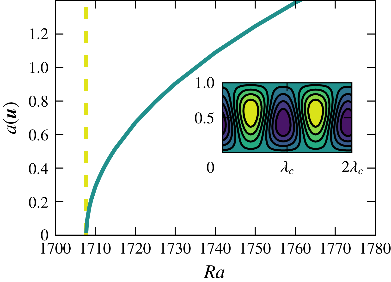
Bifurcation diagram of the Rayleigh–Bénard instability. The dashed yellow line marks the position for the theoretical critical Rayleigh number and the solid line shows the amplitude
 $a(\boldsymbol{u})$
of the convection solution. The inset shows the temperature field (deviation from conduction state) of the convection solutions at
 $Ra=1880$
.

To test our implementation several qualitative and quantitative test were performed. We calculated the critical Reynolds number of Rayleigh–Bénard-convection and compared our result to the known literature value
 $Ra=1707.76$
(Busse Reference Busse1978). A calculated bifurcation diagram for the critical wavenumber is shown in figure 18. The relative error in the critical Rayleigh number obtained with the code compared to the literature value was of order
 $10^{-5}$
. As a further (qualitative) test we considered sheared convection. Following the work of Clever & Busse (Reference Clever and Busse1992), the ECS in isothermal plane Couette flow was continued in Rayleigh number and shown to connect to the roll solution created by the thermal instability.