1 Introduction
In the past few decades, research on the interaction between water waves and sea ice has received a considerable amount of interest. Ice sheets have usually been modelled by elastic plates resting on water. A notable example of such problems is the propagation of water waves into a semi-infinite ice sheet floating on water. Evans & Davies (Reference Evans and Davies1968) obtained an explicit solution based on a thin-plate theory by using the Wiener–Hopf technique. Fox & Squire (Reference Fox and Squire1990, Reference Fox and Squire1994) adopted the method of matched eigenfunction expansion for this problem, where the conjugate gradient method was used to impose continuity conditions at the interface and edge conditions. Balmforth & Craster (Reference Balmforth and Craster1999) further extended the Evans and Davies study by applying the Wiener–Hopf technique and Fourier transforms for the thick plate model where the Timoshenko–Mindlin equation was adopted for the deflection of the ice sheet. Other works on ocean wave interaction with ice cover based on thin-plate theory can also be found in Sahoo, Yip & Chwang (Reference Sahoo, Yip and Chwang2001) based on an orthogonal mode-coupling relation which has been further expanded by Manam, Bhattacharjee & Sahoo (Reference Manam, Bhattacharjee and Sahoo2006) and Mondal, Mohanty & Sahoo (Reference Mondal, Mohanty and Sahoo2011), and can be found in Chung & Fox (Reference Chung and Fox2002) based on the Wiener–Hopf technique, in Andrianov & Hermans (Reference Andrianov and Hermans2003) based on the Green’s function technique, in Meylan & Squire (Reference Meylan and Squire1996) for a circular ice floe and in recent work by Porter (Reference Porter2019) for a rectangular ice sheet.
Large stress and strains in ice may cause fracture and cracks, which can have an obvious influence on the wave flow field. Squire & Dixon (Reference Squire and Dixon2000) considered incident waves propagating through a solitary crack of an ice sheet on water of infinite depth. Evans & Porter (Reference Evans and Porter2003) solved a more general problem of arbitrary water depth. Further investigations were made by Porter & Evans (Reference Porter and Evans2006, Reference Porter and Evans2007) by considering multiple straight narrow parallel cracks of infinite and finite lengths. Wave diffraction by a three-dimensional circular crack was studied by Li, Wu & Shi (Reference Li, Wu and Shi2018). Other water wave–ice interaction problems associated with polynyas and the marginal ice zone (MIZ) have also received a lot of attention from researchers, and a review of these studies can be found in a recent paper by Squire (Reference Squire2020).
Different from the above studies, where the ice sheet is usually treated as unbounded, which can be realistic in polar oceans, there is also an interest in wave/ice sheet interaction in confined regions such as in a river or channel. During the winter season in cold regions, the water surface in a channel may be frozen and covered by an ice sheet. The propagation of hydroelastic waves in ice-covered channels is quite different from free surface waves in an open water channel (Chang, Melville & Miles Reference Chang, Melville and Miles1979; Witting Reference Witting1984; Ertekin, Webster & Wehausen Reference Ertekin, Webster and Wehausen1986; Mathew & Akylas Reference Mathew and Akylas1990; Winckler & Liu Reference Winckler and Liu2015). For waves travelling under an infinitely long ice sheet in a wide channel, when the connection between the ice cover with the channel sides is neglected, the flow in the channel can be simplified as one-dimensional. Daly (Reference Daly1993) investigated the unsteady flow in an ice-covered channel of rectangular section by solving three linearized governing equations respectively for the mass, momentum conservation of the fluid and the motion of ice plate. Daly (Reference Daly1995) further studied the stresses induced in the ice due to its elastic deformation when water waves were travelling below. Xia & Shen (Reference Xia and Shen2002) considered the nonlinear interaction using a fifth-order Korteweg–de Vries equation for the ice cover in a channel. Beltaos (Reference Beltaos2004) involved the free edge conditions of zero bending moment and shear force in an analysis for waves passing a transverse crack across the channel. Fuamba, Bouaanani & Marche (Reference Fuamba, Bouaanani and Marche2007) investigated dam break water wave propagation in a partially ice-covered channel numerically and experimentally. A numerical model was proposed with a combination of one-dimensional Saint-Venant equations for the free surface flow and water hammer equations for the flow beneath the ice cover. Nzokou, Morse & Quach-Thanh (Reference Nzokou, Morse and Quach-Thanh2009) considered the two-dimensional wave propagation in a channel with ice cover by assuming the ice sheet to be frozen into or simply attached to the channel banks. Later, Nzokou et al. (Reference Nzokou, Morse, Robert, Richard and Tossou2011) developed a coupled model involving the one-dimensional Saint-Venant equations and the dynamic beam equation, in which a finite element method was used to solve the fluid and beam equations separately.
A more recent work done by Korobkin, Khabakhpasheva & Papin (Reference Korobkin, Khabakhpasheva and Papin2014) reconsidered waves propagating along a rectangular channel fully covered by a continuous ice sheet clamped into the channel walls, based on the linearized velocity potential theory for fluid flow and the thin-plate elastic theory for the ice sheet. The Laplace equation for the fluid flow is solved using eigenfunction expansion with each term satisfying the channel wall and bottom conditions. For the ice sheet, the solution for the Euler–Bernoulli plate equation is also expanded into a series with each term satisfying the clamped edge condition. Therefore, the transverse Fourier expansions for the fluid and the transverse expansion for the ice sheet have different eigenfunctions. When the dynamic and kinematic conditions on the interface of the fluid and ice are imposed, it is not straightforward to match these two different eigenfunctions. Each term in the expansion for the ice sheet is then further expanded into Fourier series to match the expansion for the fluid flow. Therefore, the procedures are not the most effective for this problem. Apart from the problem caused by the above-mentioned mismatch of the eigenfunctions, as they have mentioned in their conclusion, the orthonormal modes adopted are only for the clamped–clamped edge condition. When the edge conditions are changed, the suitable modes for the plate deflection need to be rederived and the problem has to be resolved; for example, the corresponding free edge problem was considered later by Batyaev & Khabakhpasheva (Reference Batyaev and Khabakhpasheva2015). It should also be mentioned that the formulation would have to be rederived for more general cases, such as an ice sheet with a crack.
In a channel, wave–ice sheet interaction occurs within a confined region between the channel walls whose effects as well as the edge constraints of ice cover on the walls cannot be ignored. The importance of sidewall effects on a body floating on the free surface are well known and to account for these effects in the solution procedure is a major challenge (e.g. Linton & Evans Reference Linton and Evans1992; Wu Reference Wu1998). The problem is further complicated by the ice sheet on the water surface, which is evidently reflected by the work of Korobkin et al. (Reference Korobkin, Khabakhpasheva and Papin2014). Apart from mathematical modelling, there have been physical tests in an ice tank. Examples include that by Dolatshah et al. (Reference Dolatshah, Nelli, Bennetts, Alberello, Meylan, Monty and Toffoli2018) for wave and ice sheet interactions and that by Myland & Ehlers (Reference Myland and Ehlers2019) with structures. The problem of a wave in an ice tank is of real physical interest as well as mathematical interest. Therefore, we aim to develop an effective and general procedure to solve this type of hydroelastic problem of a channel covered by the ice sheet with or without a crack, and with various edge conditions at the channel banks. The procedure enables us to use a series of cosine functions for the expansion of the velocity potential, as well as the ice deflection. This removes the difficulty of the mismatching mentioned above and allows us to solve a variety of the problems effectively. In the present work, we first apply this novel method to study the wave propagation in a channel with a continuous ice cover with an arbitrary combination of edge conditions at the channel banks. Then, we further consider a longitudinal crack in the ice sheet, through introducing the Dirac delta function and its derivatives at the crack to the equation. This enables us to enforce the conditions at the crack easily and there is no need to redrive the formulation. Because of the simplicity of the solution procedure, we are able to uncover some insights into the nature of wave propagation in an ice-covered channel with or without a crack.
The paper is organized as follows. The mathematical model and solution procedure for water waves interacting with a continuous ice cover are developed in § 2. For the discontinuous situation, the procedure is extended in § 3 for ice cover with a longitudinal straight-line crack at an arbitrary position. Extensive results are provided in § 4 for dispersion relations, wave celerity, wave deflection and strain in the ice for different combinations of edge conditions at the channel banks with or without a crack, and in-depth discussions are made. Conclusions are given in § 5.
2 Mathematical formulation and solution procedure for a continuous ice sheet
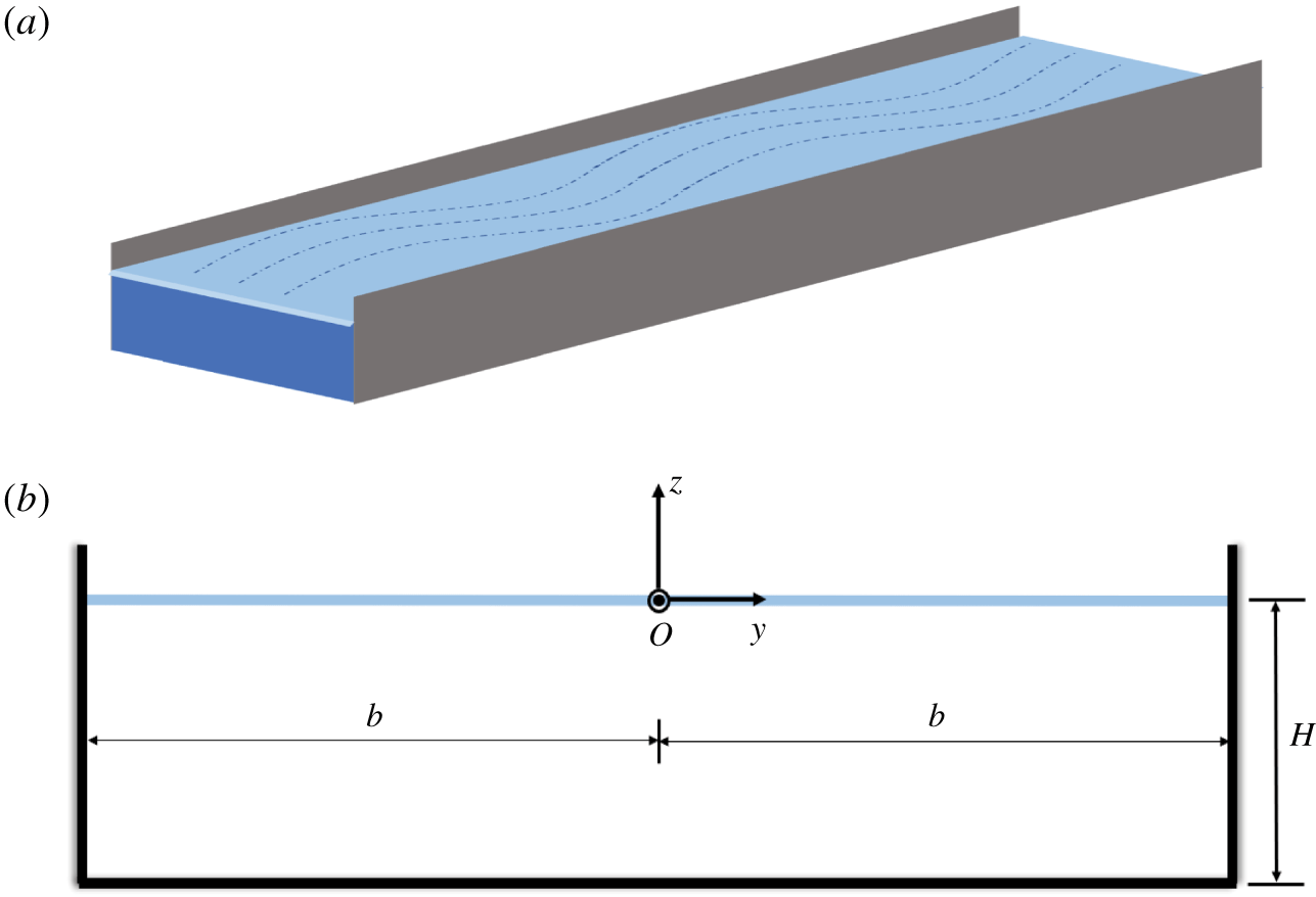
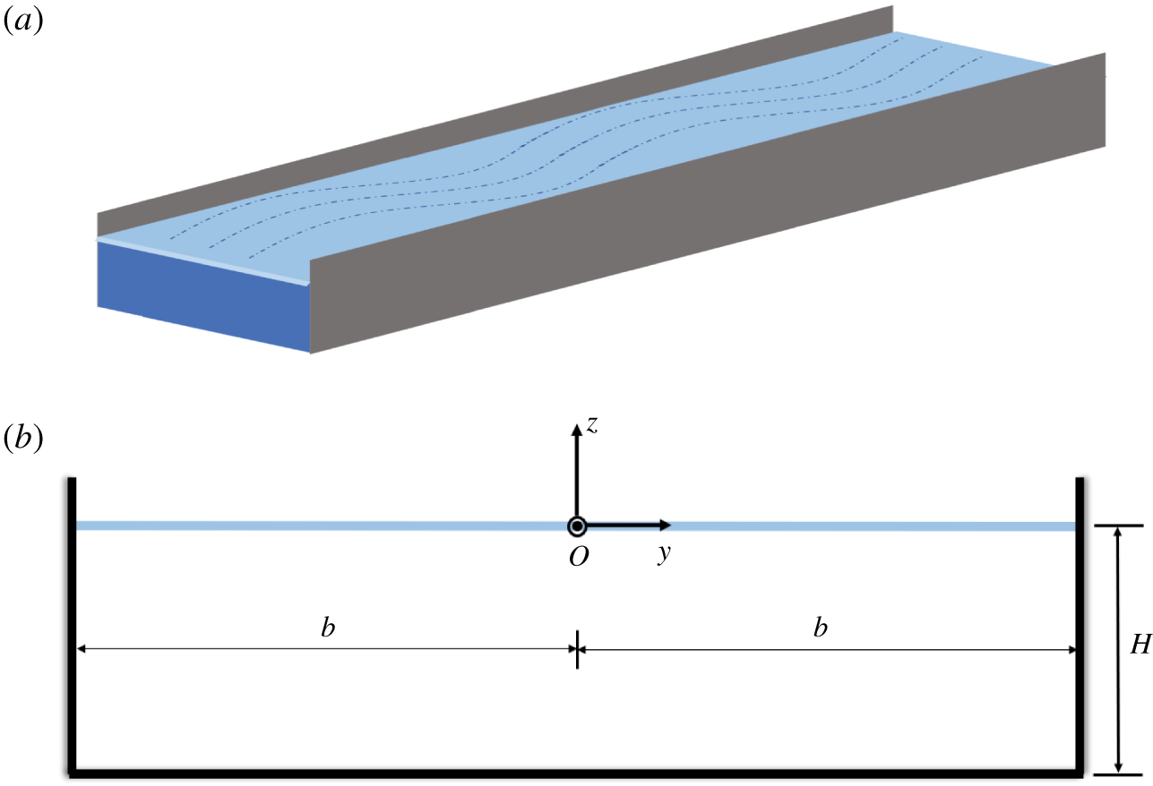
The problem is shown in figure 1. A channel of rectangular section is covered by a homogeneous ice sheet. The half-width of the channel and the water depth are denoted as  $b$ and
 $H$, respectively. A Cartesian coordinate system
 $Oxyz$ is defined with the origin located at the lower surface of the ice sheet and the central plane of the channel, the
 $x$-axis points in the longitudinal direction of the channel and the
 $z$-axis points upwards. The linearized incompressible velocity potential theory is used for the fluid flow. The potential
 $\unicode[STIX]{x1D719}(x,y,z,t)$ satisfies the Laplace equation as
Sketch of the hydroelastic wave propagation in a rectangular channel covered by ice sheet. (a) Three-dimensional view; (b) view for cross-section of the channel in which  $x$-axis points out of the paper.
 $$\begin{eqnarray}\unicode[STIX]{x1D6FB}^{2}\unicode[STIX]{x1D719}=\frac{\unicode[STIX]{x2202}^{2}\unicode[STIX]{x1D719}}{\unicode[STIX]{x2202}x^{2}}+\frac{\unicode[STIX]{x2202}^{2}\unicode[STIX]{x1D719}}{\unicode[STIX]{x2202}y^{2}}+\frac{\unicode[STIX]{x2202}^{2}\unicode[STIX]{x1D719}}{\unicode[STIX]{x2202}z^{2}}=0,\quad -\infty <x<+\infty ,-b\leqslant y\leqslant b,-H\leqslant z\leqslant 0,\end{eqnarray}$$
in the entire fluid domain of the channel, while the impermeable conditions are satisfied on the channel walls and bottom, which give
 $$\begin{eqnarray}\frac{\unicode[STIX]{x2202}\unicode[STIX]{x1D719}}{\unicode[STIX]{x2202}y}=0,\quad y=\pm b;\quad \frac{\unicode[STIX]{x2202}\unicode[STIX]{x1D719}}{\unicode[STIX]{x2202}z}=0,\quad z=-H.\end{eqnarray}$$
The deflection of the ice sheet  $w(x,y,t)$ is governed by the Euler–Bernoulli equation as
 $$\begin{eqnarray}\unicode[STIX]{x1D70C}_{i}h_{i}w_{tt}+L\unicode[STIX]{x1D6FB}^{4}w=p,\end{eqnarray}$$
where  $\unicode[STIX]{x1D70C}_{i}$ is the density of the ice sheet,
 $h_{i}$ is its thickness,
 $L=Eh_{i}^{3}/[12(1-\unicode[STIX]{x1D708}^{2})]$ is the rigidity coefficient with
 $E$ and
 $\unicode[STIX]{x1D708}$ being the Young’s modulus and Poisson’s ratio of the ice sheet, respectively. The term on the right-hand side of (2.3) is the fluid pressure, which can be obtained from the linearized Bernoulli equation, or
 $p=-\unicode[STIX]{x1D70C}\unicode[STIX]{x1D719}_{t}-\unicode[STIX]{x1D70C}gw$, where
 $\unicode[STIX]{x1D70C}$ is the density of water and
 $g$ is the acceleration due to gravity. The kinematic condition is
 $$\begin{eqnarray}\frac{\unicode[STIX]{x2202}w}{\unicode[STIX]{x2202}t}=\frac{\unicode[STIX]{x2202}\unicode[STIX]{x1D719}}{\unicode[STIX]{x2202}z},\quad z=0.\end{eqnarray}$$
Considering a periodic wave in both time and the  $x$ direction, the deflection of the ice sheet and the velocity potential can be written as
 $$\begin{eqnarray}\displaystyle & \displaystyle w(x,y,t)=\text{Re}\{W(y)\text{e}^{\text{i}(\unicode[STIX]{x1D705}x-\unicode[STIX]{x1D714}t)}\},\quad -b\leqslant y\leqslant b, & \displaystyle\end{eqnarray}$$
 $$\begin{eqnarray}\displaystyle & \displaystyle \unicode[STIX]{x1D719}(x,y,z,t)=\text{Re}\{-\text{i}\unicode[STIX]{x1D714}\unicode[STIX]{x1D6F7}(y,z)\text{e}^{\text{i}(\unicode[STIX]{x1D705}x-\unicode[STIX]{x1D714}t)}\},\quad -b\leqslant y\leqslant b,-H\leqslant z\leqslant 0, & \displaystyle\end{eqnarray}$$
where  $\unicode[STIX]{x1D705}$ is the wavenumber and
 $\unicode[STIX]{x1D714}$ is the frequency. Using (2.5) and (2.6), the dynamic equation of the ice sheet in (2.3) can be written as
 $$\begin{eqnarray}-\unicode[STIX]{x1D714}^{2}\unicode[STIX]{x1D70C}_{i}h_{i}W+L(\unicode[STIX]{x1D705}^{4}W-2\unicode[STIX]{x1D705}^{2}W^{\prime \prime }+W^{\prime \prime \prime \prime })=\unicode[STIX]{x1D70C}\unicode[STIX]{x1D714}^{2}\unicode[STIX]{x1D6F7}(y,0)-\unicode[STIX]{x1D70C}gW,\end{eqnarray}$$
and from the kinematic condition, we can have
 $$\begin{eqnarray}W(y)=\unicode[STIX]{x1D6F7}_{z}(y,0).\end{eqnarray}$$
Taking into account the impermeable conditions on the channel bottom and wall, we can further write the expression of the potential  $\unicode[STIX]{x1D6F7}(y,z)$ as
 $$\begin{eqnarray}\unicode[STIX]{x1D6F7}(y,z)=\mathop{\sum }_{n=0}^{\infty }b_{n}\cosh k_{n}(z+H)\cos \unicode[STIX]{x1D70E}_{n}(y+b),\quad -b\leqslant y\leqslant b,\end{eqnarray}$$
where
 $$\begin{eqnarray}\unicode[STIX]{x1D70E}_{n}=\frac{n\unicode[STIX]{x03C0}}{2b},\quad k_{n}^{2}=\unicode[STIX]{x1D70E}_{n}^{2}+\unicode[STIX]{x1D705}^{2},\end{eqnarray}$$
and the choice of  $\unicode[STIX]{x1D70E}_{n}$ is due to the wall conditions at
 $y=\pm b$ and that of
 $k_{n}$ is due to the Laplace equation.
To impose (2.8), it would be much more convenient to use the same expansion for both  $W$ and
 $\unicode[STIX]{x1D6F7}$. However, to use a Fourier cosine series directly for
 $W$ would lead to two problems: (i) The term in the series of
 $W$ cannot satisfy all the four edge conditions. The conditions have to be imposed through
 $W$ separately, which is not a trivial task. (ii) The Fourier series is not always differentiable but is integrable. Therefore, we expand
 $W^{\prime \prime \prime \prime }$ into a cosine series, which does not have to care about the edge conditions at this stage:
 $$\begin{eqnarray}W^{\prime \prime \prime \prime }(y)=\mathop{\sum }_{n=0}^{\infty }a_{n}\cos \unicode[STIX]{x1D70E}_{n}(y+b),\quad -b\leqslant y\leqslant b\end{eqnarray}$$
when it is integrated, the general expansion of  $W(y)$ becomes
 $$\begin{eqnarray}W(y)=c_{0}+c_{1}(y+b)+c_{2}(y+b)^{2}+c_{3}(y+b)^{3}+\frac{a_{0}}{24}(y+b)^{4}+\mathop{\sum }_{n=1}^{\infty }\frac{a_{n}}{\unicode[STIX]{x1D70E}_{n}^{4}}\cos \unicode[STIX]{x1D70E}_{n}(y+b),\end{eqnarray}$$
where  $c_{i}\,(i=0\sim 3)$ are four constants. They can be written in terms of
 $a_{n}$ based on the specific four edge conditions. This means that, unlike the expansion of the potential, not every term in (2.12) satisfies the edge conditions, but
 $W(y)$ itself does. From (2.12), we can find that
 $c_{0}$,
 $c_{1}$,
 $c_{2}$,
 $c_{3}$ have the same dimensions as those of deflection, slope, bending moment and shear force, respectively. Specifically, we have
 $c_{1}=W^{\prime }(-b)$ and
 $c_{3}=(1/6)W^{\prime \prime \prime }(-b)$.
Substituting (2.9) and (2.12) into (2.7) and (2.8) respectively, we have
 $$\begin{eqnarray}\displaystyle & & \displaystyle (\unicode[STIX]{x1D70C}g-\unicode[STIX]{x1D714}^{2}\unicode[STIX]{x1D70C}_{i}h_{i}+L\unicode[STIX]{x1D705}^{4})\nonumber\\ \displaystyle & & \displaystyle \quad \times \,\left[\mathop{\sum }_{n=1}^{\infty }\frac{a_{n}}{\unicode[STIX]{x1D70E}_{n}^{4}}\cos \unicode[STIX]{x1D70E}_{n}(y+b)+\frac{a_{0}}{24}(y+b)^{4}+c_{3}(y+b)^{3}+c_{2}(y+b)^{2}+c_{1}(y+b)+c_{0}\right]\nonumber\\ \displaystyle & & \displaystyle \quad -\,2\unicode[STIX]{x1D705}^{2}L\left[-\mathop{\sum }_{n=1}^{\infty }\frac{a_{n}}{\unicode[STIX]{x1D70E}_{n}^{2}}\cos \unicode[STIX]{x1D70E}_{n}(y+b)+\frac{a_{0}}{2}(y+b)^{2}+6c_{3}(y+b)+2c_{2}\right]\nonumber\\ \displaystyle & & \displaystyle \quad +\,L\mathop{\sum }_{n=0}^{\infty }a_{n}\cos \unicode[STIX]{x1D70E}_{n}(y+b)=\unicode[STIX]{x1D70C}\unicode[STIX]{x1D714}^{2}\mathop{\sum }_{n=0}^{\infty }b_{n}\cosh k_{n}H\cos \unicode[STIX]{x1D70E}_{n}(y+b),\end{eqnarray}$$
 $$\begin{eqnarray}\displaystyle & & \displaystyle \mathop{\sum }_{n=1}^{\infty }\frac{a_{n}}{\unicode[STIX]{x1D70E}_{n}^{4}}\cos \unicode[STIX]{x1D70E}_{n}(y+b)+\frac{a_{0}}{24}(y+b)^{4}+c_{3}(y+b)^{3}+c_{2}(y+b)^{2}+c_{1}(y+b)+c_{0}\nonumber\\ \displaystyle & & \displaystyle \quad =\,\mathop{\sum }_{n=0}^{\infty }b_{n}k_{n}\sinh k_{n}H\cos \unicode[STIX]{x1D70E}_{n}(y+b).\end{eqnarray}$$
We may further expand functions of  $(y+b)^{j}(j=0\sim 4)$ into the orthogonal series of cosine functions as
 $$\begin{eqnarray}(y+b)^{j}=\mathop{\sum }_{n=0}^{\infty }d_{n}^{(j)}\cos \unicode[STIX]{x1D70E}_{n}(y+b).\end{eqnarray}$$
Equations (2.13) and (2.14) then give
 $$\begin{eqnarray}\displaystyle & & \displaystyle (\unicode[STIX]{x1D70C}g-\unicode[STIX]{x1D714}^{2}\unicode[STIX]{x1D70C}_{i}h_{i}+L\unicode[STIX]{x1D705}^{4})\left(\frac{(1-\unicode[STIX]{x1D6FF}_{n0})a_{n}}{\unicode[STIX]{x1D70E}_{n}^{4}}+\frac{a_{0}}{24}d_{n}^{(4)}+c_{3}d_{n}^{(3)}+c_{2}d_{n}^{(2)}+c_{1}d_{n}^{(1)}+c_{0}d_{n}^{(0)}\right)\nonumber\\ \displaystyle & & \displaystyle \qquad -\,2\unicode[STIX]{x1D705}^{2}L\left(-\frac{(1-\unicode[STIX]{x1D6FF}_{n0})a_{n}}{\unicode[STIX]{x1D70E}_{n}^{2}}+\frac{a_{0}}{2}d_{n}^{(2)}+6c_{3}d_{n}^{(1)}+2c_{2}d_{n}^{(0)}\right)+La_{n}\nonumber\\ \displaystyle & & \displaystyle \quad =\unicode[STIX]{x1D70C}\unicode[STIX]{x1D714}^{2}b_{n}\cosh k_{n}H,\quad n=0,1,2,\ldots ,\end{eqnarray}$$
 $$\begin{eqnarray}\frac{(1-\unicode[STIX]{x1D6FF}_{n0})a_{n}}{\unicode[STIX]{x1D70E}_{n}^{4}}+\frac{a_{0}}{24}d_{n}^{(4)}+c_{3}d_{n}^{(3)}+c_{2}d_{n}^{(2)}+c_{1}d_{n}^{(1)}+c_{0}d_{n}^{(0)}=b_{n}k_{n}\sinh k_{n}H,\quad n=0,1,2,\ldots ,\end{eqnarray}$$
where  $\unicode[STIX]{x1D6FF}_{ij}$ is the Kronecker delta function. From these two equations, we obtain
 $$\begin{eqnarray}\displaystyle & \displaystyle a_{n}=\unicode[STIX]{x1D6FC}_{n3}c_{3}+\unicode[STIX]{x1D6FC}_{n2}c_{2}+\unicode[STIX]{x1D6FC}_{n1}c_{1}+\unicode[STIX]{x1D6FC}_{n0}c_{0}, & \displaystyle\end{eqnarray}$$
 $$\begin{eqnarray}\displaystyle & \displaystyle b_{n}=\unicode[STIX]{x1D6FD}_{n3}c_{3}+\unicode[STIX]{x1D6FD}_{n2}c_{2}+\unicode[STIX]{x1D6FD}_{n1}c_{1}+\unicode[STIX]{x1D6FD}_{n0}c_{0}, & \displaystyle\end{eqnarray}$$
where
 $$\begin{eqnarray}\displaystyle \displaystyle \unicode[STIX]{x1D6E5}_{n} & = & \displaystyle \displaystyle \unicode[STIX]{x1D6FF}_{n0}\left[-k_{0}\sinh k_{0}H\left(\frac{(\unicode[STIX]{x1D70C}g-\unicode[STIX]{x1D714}^{2}\unicode[STIX]{x1D70C}_{i}h_{i}+L\unicode[STIX]{x1D705}^{4})d_{0}^{(4)}}{24}-\unicode[STIX]{x1D705}^{2}Ld_{0}^{(2)}+L\right)\right.\nonumber\\ \displaystyle & & \displaystyle \displaystyle +\left.\frac{d_{0}^{(4)}\unicode[STIX]{x1D70C}\unicode[STIX]{x1D714}^{2}\cosh k_{0}H}{24}\right]+(1-\unicode[STIX]{x1D6FF}_{n0})\left[-k_{n}\sinh k_{n}H\vphantom{\frac{\unicode[STIX]{x1D70C}-\unicode[STIX]{x1D714}^{2}}{\unicode[STIX]{x1D70E}_{n}^{4}}}\right.\nonumber\\ \displaystyle & & \displaystyle \displaystyle \left.\left(\frac{\unicode[STIX]{x1D70C}g-\unicode[STIX]{x1D714}^{2}\unicode[STIX]{x1D70C}_{i}h_{i}+L\unicode[STIX]{x1D705}^{4}}{\unicode[STIX]{x1D70E}_{n}^{4}}+\frac{2\unicode[STIX]{x1D705}^{2}L}{\unicode[STIX]{x1D70E}_{n}^{2}}+L\right)+\frac{\unicode[STIX]{x1D70C}\unicode[STIX]{x1D714}^{2}\cosh k_{n}H}{\unicode[STIX]{x1D70E}_{n}^{4}}\right],\end{eqnarray}$$
 $$\begin{eqnarray}\displaystyle \unicode[STIX]{x1D6FC}_{nj} & = & \displaystyle \displaystyle \frac{1}{\unicode[STIX]{x1D6E5}_{n}}\left\{d_{n}^{(j)}[(\unicode[STIX]{x1D70C}g-\unicode[STIX]{x1D714}^{2}\unicode[STIX]{x1D70C}_{i}h_{i}+L\unicode[STIX]{x1D705}^{4})k_{n}\sinh k_{n}H-\unicode[STIX]{x1D70C}\unicode[STIX]{x1D714}^{2}\cosh k_{n}H]\right.\nonumber\\ \displaystyle & & \displaystyle \displaystyle -\,12\unicode[STIX]{x1D6FF}_{j3}\unicode[STIX]{x1D705}^{2}Ld_{n}^{(1)}k_{n}\sinh k_{n}H-4\unicode[STIX]{x1D6FF}_{j2}\unicode[STIX]{x1D705}^{2}Ld_{n}^{(0)}k_{n}\sinh k_{n}H+(1-\unicode[STIX]{x1D6FF}_{n0})\unicode[STIX]{x1D6FC}_{0j}\nonumber\\ \displaystyle & & \displaystyle \displaystyle \times \,\left[\left(\frac{(\unicode[STIX]{x1D70C}g-\unicode[STIX]{x1D714}^{2}\unicode[STIX]{x1D70C}_{i}h_{i}+L\unicode[STIX]{x1D705}^{4})d_{n}^{(4)}}{24}-\unicode[STIX]{x1D705}^{2}Ld_{n}^{(2)}\right)k_{n}\sinh k_{n}H\right.\nonumber\\ \displaystyle & & \displaystyle \displaystyle -\left.\left.\frac{d_{n}^{(4)}\unicode[STIX]{x1D70C}\unicode[STIX]{x1D714}^{2}\cosh k_{n}H}{24}\right]\right\},\end{eqnarray}$$
 $$\begin{eqnarray}\displaystyle \unicode[STIX]{x1D6FD}_{nj} & = & \displaystyle \displaystyle \frac{\unicode[STIX]{x1D6FF}_{n0}L}{\unicode[STIX]{x1D6E5}_{n}}\left[-(1-\unicode[STIX]{x1D705}^{2}d_{0}^{(2)})d_{0}^{(j)}-\frac{\unicode[STIX]{x1D6FF}_{3j}\unicode[STIX]{x1D705}^{2}d_{0}^{(1)}d_{0}^{(4)}}{2}-\frac{\unicode[STIX]{x1D6FF}_{2j}\unicode[STIX]{x1D705}^{2}d_{0}^{(0)}d_{0}^{(4)}}{6}\right]+\frac{(1-\unicode[STIX]{x1D6FF}_{n0})L}{\unicode[STIX]{x1D6E5}_{n}}\nonumber\\ \displaystyle & & \displaystyle \displaystyle \times \,\left[-\left(\frac{2\unicode[STIX]{x1D705}^{2}}{\unicode[STIX]{x1D70E}_{n}^{2}}+1\right)d_{n}^{(j)}-\frac{12\unicode[STIX]{x1D6FF}_{j3}\unicode[STIX]{x1D705}^{2}d_{n}^{(1)}}{\unicode[STIX]{x1D70E}_{n}^{4}}-\frac{4\unicode[STIX]{x1D6FF}_{j2}\unicode[STIX]{x1D705}^{2}d_{n}^{(0)}}{\unicode[STIX]{x1D70E}_{n}^{4}}\right.\nonumber\\ \displaystyle & & \displaystyle \displaystyle +\left.\unicode[STIX]{x1D6FC}_{0j}\left(-\frac{d_{n}^{(4)}}{24}\left(\frac{2\unicode[STIX]{x1D705}^{2}}{\unicode[STIX]{x1D70E}_{n}^{2}}+1\right)-\frac{\unicode[STIX]{x1D705}^{2}d_{n}^{(2)}}{\unicode[STIX]{x1D70E}_{n}^{4}}\right)\right](j=0\sim 3,n=0,1,2\ldots ).\end{eqnarray}$$
In (2.18) and (2.19),  $\unicode[STIX]{x1D6FC}_{nj}$ and
 $\unicode[STIX]{x1D6FD}_{nj}$ are known. These two systems of equations become complete when the edge conditions are used. For clamped, free and simply supported conditions, we respectively have at edge (Timoshenko & Woinowsky-Krieger Reference Timoshenko and Woinowsky-Krieger1959)
 $$\begin{eqnarray}W=W^{\prime }=0,\end{eqnarray}$$
 $$\begin{eqnarray}W^{\prime \prime }-\unicode[STIX]{x1D708}\unicode[STIX]{x1D705}^{2}W=0,\quad W^{\prime \prime \prime }-(2-\unicode[STIX]{x1D708})\unicode[STIX]{x1D705}^{2}W^{\prime }=0,\end{eqnarray}$$
 $$\begin{eqnarray}W=0,\quad W^{\prime \prime }-\unicode[STIX]{x1D708}\unicode[STIX]{x1D705}^{2}W=0,\end{eqnarray}$$
where (2.5) has been used.
We may use the above procedure for the case with both edges clamped, as considered by Korobkin et al. (Reference Korobkin, Khabakhpasheva and Papin2014). In such a case, (2.21) should be used for both  $y=\pm b$. Using (2.12), we obtain
 $$\begin{eqnarray}\left.\begin{array}{@{}c@{}}\displaystyle \mathop{\sum }_{n=1}^{\infty }\frac{a_{n}}{\unicode[STIX]{x1D70E}_{n}^{4}}+c_{0}=0;\\ \displaystyle c_{1}=0;\\ \displaystyle \mathop{\sum }_{n=1}^{\infty }\frac{a_{n}}{\unicode[STIX]{x1D70E}_{n}^{4}}\cos n\unicode[STIX]{x03C0}+\frac{2b^{4}}{3}a_{0}+8b^{3}c_{3}+4b^{2}c_{2}+2bc_{1}+c_{0}=0;\\ \displaystyle \frac{4b^{3}}{3}a_{0}+12b^{2}c_{3}+4bc_{2}+c_{1}=0.\end{array}\right\}\end{eqnarray}$$
Dividing (2.18) by  $\unicode[STIX]{x1D70E}_{n}^{4}$, performing the summation and substituting the result into (2.24), we have
 $$\begin{eqnarray}[\boldsymbol{A}][\boldsymbol{C}]=0,\end{eqnarray}$$
where  $\boldsymbol{C}$ is a column containing
 $c_{i}$. For practical calculation, the infinite series in (2.25) needs to be truncated at a finite number. In general
 $\boldsymbol{A}$ is a
 $4\times 4$ coefficient matrix (see appendix A). For the clamped condition, it can be further simplified into
 $3\times 3$ because
 $c_{1}=0$ is already obtained. For non-trivial solution of
 $\boldsymbol{C}$, we should have
 $|\boldsymbol{A}|=0$. This provides the dispersion relationship between
 $\unicode[STIX]{x1D705}$ and
 $\unicode[STIX]{x1D714}$, or at each given
 $\unicode[STIX]{x1D705}$, we obtain various
 $\unicode[STIX]{x1D714}$ which are the natural frequencies of the frozen channel. It should be noted that, from the dispersion relationship for an ice sheet of infinite extent (e.g. Fox & Squire Reference Fox and Squire1994), the wavenumber for a travelling wave is unique at each frequency. Here, at each
 $\unicode[STIX]{x1D714}$,
 $\unicode[STIX]{x1D705}$ is not unique. In fact, there is an infinite number of solutions of
 $\unicode[STIX]{x1D705}$, which can be obtained from
 $|\boldsymbol{A}|=0$ in (2.25). Each
 $\unicode[STIX]{x1D705}$ corresponds to a different travelling wave along the channel and different transverse waves across the channel. At each of these particular frequencies, we may choose one
 $c_{i}$, and then solve (2.25) to obtain other
 $c_{i}$ and to obtain
 $a_{n}$ and
 $b_{n}$ from (2.18) and (2.19), respectively. This will then provide all the transverse modes for both the fluid flow in (2.9) and ice sheet deflection in (2.12). For other combinations of edge conditions in (2.21)–(2.23), the same procedure as (2.24) and (2.25) can be obtained. The only difference is then in the coefficients of
 $\boldsymbol{A}$.
3 Ice sheet with a longitudinal straight-line crack
The formulation above can be extended to the case of ice sheet with a longitudinal straight-line crack at  $y=l$. In such a case
 $W(y)$ will not be continuous at
 $y=l$. We denote two smooth functions, namely
 $W_{1}(y)$ and
 $W_{2}(y)$, as the deflections of the beam on two sides of the crack. Then the deflection of the entire beam can be written as (Wang & Qiao Reference Wang and Qiao2007)
 $$\begin{eqnarray}W(y)=W_{1}(y)+[W_{2}(y)-W_{1}(y)]\text{H}(y-l),\end{eqnarray}$$
where  $\text{H}(y-l)$ is the Heaviside step function. Substituting (3.1) and its derivatives into (2.7), we could modify the dynamic equation as
 $$\begin{eqnarray}\displaystyle & & \displaystyle -\unicode[STIX]{x1D714}^{2}\unicode[STIX]{x1D70C}_{i}h_{i}W+L(\unicode[STIX]{x1D705}^{4}W-2\unicode[STIX]{x1D705}^{2}W^{\prime \prime }+W^{\prime \prime \prime \prime })\nonumber\\ \displaystyle & & \displaystyle \quad =\unicode[STIX]{x1D70C}\unicode[STIX]{x1D714}^{2}\unicode[STIX]{x1D6F7}(y,0)-\unicode[STIX]{x1D70C}gW+L[\unicode[STIX]{x0394}W^{\prime \prime \prime }(l)-2\unicode[STIX]{x1D705}^{2}\unicode[STIX]{x0394}W^{\prime }(l)]\cdot \unicode[STIX]{x1D6FF}(y-l)\nonumber\\ \displaystyle & & \displaystyle \qquad +\,L[\unicode[STIX]{x0394}W^{\prime \prime }(l)-2\unicode[STIX]{x1D705}^{2}\unicode[STIX]{x0394}W(l)]\cdot \unicode[STIX]{x1D6FF}^{\prime }(y-l)+L\unicode[STIX]{x0394}W^{\prime }(l)\cdot \unicode[STIX]{x1D6FF}^{\prime \prime }(y-l)\nonumber\\ \displaystyle & & \displaystyle +\,L\unicode[STIX]{x0394}W(l)\cdot \unicode[STIX]{x1D6FF}^{\prime \prime \prime }(y-l),\end{eqnarray}$$
where  $\unicode[STIX]{x0394}W(l)$,
 $\unicode[STIX]{x0394}W^{\prime }(l)$,
 $\unicode[STIX]{x0394}W^{\prime \prime }(l)$ and
 $\unicode[STIX]{x0394}W^{\prime \prime \prime }(l)$ are respectively the jumps of the deflection, slope, the second and third derivatives of
 $W$ at the crack and
 $\unicode[STIX]{x1D6FF}(y-l)$,
 $\unicode[STIX]{x1D6FF}^{\prime }(y-l)$,
 $\unicode[STIX]{x1D6FF}^{\prime \prime }(y-l)$ and
 $\unicode[STIX]{x1D6FF}^{\prime \prime \prime }(y-l)$ are respectively the Dirac delta function and its derivatives with respect to
 $y$.
When free edge conditions are assumed on both sides of the crack, indicating zero bending moment and shear force, then (2.22) should be satisfied at  $y=l$ as
 $$\begin{eqnarray}\left.\begin{array}{@{}c@{}}W^{\prime \prime }(l^{-})-\unicode[STIX]{x1D708}\unicode[STIX]{x1D705}^{2}W(l^{-})=W^{\prime \prime }(l^{+})-\unicode[STIX]{x1D708}\unicode[STIX]{x1D705}^{2}W(l^{+})=0,\\ W^{\prime \prime \prime }(l^{-})-(2-\unicode[STIX]{x1D708})\unicode[STIX]{x1D705}^{2}W^{\prime }(l^{-})=W^{\prime \prime \prime }(l^{+})-(2-\unicode[STIX]{x1D708})\unicode[STIX]{x1D705}^{2}W^{\prime }(l^{+})=0,\end{array}\right\}\end{eqnarray}$$
where  $l^{-}$ and
 $l^{+}$ in (3.3) refer to the left- and right-hand sides of
 $l$, respectively. From (3.3), we can further have
 $$\begin{eqnarray}\unicode[STIX]{x0394}W^{\prime \prime }(l)=\unicode[STIX]{x1D708}\unicode[STIX]{x1D705}^{2}\unicode[STIX]{x0394}W(l),\quad \unicode[STIX]{x0394}W^{\prime \prime \prime }(l)=(2-\unicode[STIX]{x1D708})\unicode[STIX]{x1D705}^{2}\unicode[STIX]{x0394}W^{\prime }(l).\end{eqnarray}$$
Substituting (3.4) into (3.2), we can have
 $$\begin{eqnarray}\displaystyle & & \displaystyle -\unicode[STIX]{x1D714}^{2}\unicode[STIX]{x1D70C}_{i}h_{i}W+L(\unicode[STIX]{x1D705}^{4}W-2\unicode[STIX]{x1D705}^{2}W^{\prime \prime }+W^{\prime \prime \prime \prime })\nonumber\\ \displaystyle & & \displaystyle \quad =\unicode[STIX]{x1D70C}\unicode[STIX]{x1D714}^{2}\unicode[STIX]{x1D6F7}(y,0)-\unicode[STIX]{x1D70C}gW-\unicode[STIX]{x1D708}\unicode[STIX]{x1D705}^{2}LS\cdot \unicode[STIX]{x1D6FF}(y-l)\nonumber\\ \displaystyle & & \displaystyle \qquad +\,(\unicode[STIX]{x1D708}-2)\unicode[STIX]{x1D705}^{2}LD\cdot \unicode[STIX]{x1D6FF}^{\prime }(y-l)+LS\cdot \unicode[STIX]{x1D6FF}^{\prime \prime }(y-l)+LD\cdot \unicode[STIX]{x1D6FF}^{\prime \prime \prime }(y-l),\end{eqnarray}$$
where  $S=\unicode[STIX]{x0394}W^{\prime }(l)$ and
 $D=\unicode[STIX]{x0394}W(l)$. The kinematic equation of the ice sheet will remain the same as (2.8). In (3.5), there are two extra unknowns,
 $D$ and
 $S$. Two additional equations can be obtained by the two conditions at the crack (
 $y=l$). For
 $\unicode[STIX]{x1D6FF}(y-l)$ and its derivatives, they can be written in the form of cosine series as
 $$\begin{eqnarray}\frac{\unicode[STIX]{x2202}^{k}\unicode[STIX]{x1D6FF}(y-l)}{\unicode[STIX]{x2202}y^{k}}=\mathop{\sum }_{n=0}^{\infty }\unicode[STIX]{x1D717}_{n}^{(k)}\cos \unicode[STIX]{x1D70E}_{n}(y+b),\quad k=0,1,2,3.\end{eqnarray}$$
Multiplying  $\cos \unicode[STIX]{x1D70E}_{m}(y+b)$, integrating the result with respect to
 $y$ from
 $y=-b$ to
 $y=b$ and further using the orthogonality of cosine functions and the property of the Dirac delta function, we can obtain
 $$\begin{eqnarray}\unicode[STIX]{x1D717}_{n}^{(k)}=\left\{\begin{array}{@{}ll@{}}\displaystyle \frac{\unicode[STIX]{x1D6FF}_{0k}}{2b}, & n=0\\ \displaystyle (-1)^{k}\left.\frac{\unicode[STIX]{x2202}^{k}f_{n}(y)}{\unicode[STIX]{x2202}y^{k}}\right|_{y=l}, & n\geqslant 1\end{array}\right.\end{eqnarray}$$
where  $f_{n}(y)=(\cos \unicode[STIX]{x1D70E}_{n}(y+b))/((1+\unicode[STIX]{x1D6FF}_{n0})b)$. Then (2.16) will become
 $$\begin{eqnarray}\displaystyle & & \displaystyle (\unicode[STIX]{x1D70C}g-\unicode[STIX]{x1D714}^{2}\unicode[STIX]{x1D70C}_{i}h_{i}+L\unicode[STIX]{x1D705}^{4})\left(\frac{(1-\unicode[STIX]{x1D6FF}_{n0})a_{n}}{\unicode[STIX]{x1D70E}_{n}^{4}}+\frac{a_{0}}{24}d_{n}^{(4)}+c_{3}d_{n}^{(3)}+c_{2}d_{n}^{(2)}+c_{1}d_{n}^{(1)}+c_{0}d_{n}^{(0)}\right)\nonumber\\ \displaystyle & & \displaystyle \quad -\,2\unicode[STIX]{x1D705}^{2}L\left(-\frac{(1-\unicode[STIX]{x1D6FF}_{n0})a_{n}}{\unicode[STIX]{x1D70E}_{n}^{2}}+\frac{a_{0}}{2}d_{n}^{(2)}+6c_{3}d_{n}^{(1)}+2c_{2}d_{n}^{(0)}\right)+La_{n}+(\unicode[STIX]{x1D708}\unicode[STIX]{x1D705}^{2}f_{n}(l)-f_{n}^{\prime \prime }(l))LS\nonumber\\ \displaystyle & & \displaystyle \quad +\,(-(2-\unicode[STIX]{x1D708})\unicode[STIX]{x1D705}^{2}f_{n}^{\prime }(l)+f_{n}^{\prime \prime \prime }(l))LD=\unicode[STIX]{x1D70C}\unicode[STIX]{x1D714}^{2}b_{n}\cosh k_{n}H,\quad n=0,1,2,\ldots .\end{eqnarray}$$
From (3.8) and (2.17), when considering a crack with free edges at  $y=l$, (2.18) and (2.19) would be modified as
 $$\begin{eqnarray}\displaystyle & \displaystyle a_{n}=\unicode[STIX]{x1D6FC}_{n5}S+\unicode[STIX]{x1D6FC}_{n4}D+\unicode[STIX]{x1D6FC}_{n3}c_{3}+\unicode[STIX]{x1D6FC}_{n2}c_{2}+\unicode[STIX]{x1D6FC}_{n1}c_{1}+\unicode[STIX]{x1D6FC}_{n0}c_{0}, & \displaystyle\end{eqnarray}$$
 $$\begin{eqnarray}\displaystyle & \displaystyle b_{n}=\unicode[STIX]{x1D6FD}_{n5}S+\unicode[STIX]{x1D6FD}_{n4}D+\unicode[STIX]{x1D6FD}_{n3}c_{3}+\unicode[STIX]{x1D6FD}_{n2}c_{2}+\unicode[STIX]{x1D6FD}_{n1}c_{1}+\unicode[STIX]{x1D6FD}_{n0}c_{0}. & \displaystyle\end{eqnarray}$$
When  $j\leqslant 3$,
 $\unicode[STIX]{x1D6FC}_{nj}$ and
 $\unicode[STIX]{x1D6FD}_{nj}$ are the same as those below (2.19). For
 $j=4$ and 5, we can have
 $$\begin{eqnarray}\left.\begin{array}{@{}c@{}}\displaystyle \begin{array}{@{}rcl@{}}\unicode[STIX]{x1D6FC}_{nj}\; & =\; & \displaystyle \frac{1}{\unicode[STIX]{x1D6E5}_{n}}\left\{\unicode[STIX]{x1D6FF}_{j4}Lk_{n}\sinh k_{n}H\times [-(2-\unicode[STIX]{x1D708})\unicode[STIX]{x1D705}^{2}f_{n}^{\prime }(l)+f_{n}^{\prime \prime \prime }(l)]\right.\\ \; & \; & \displaystyle +\,\unicode[STIX]{x1D6FF}_{j5}Lk_{n}\sinh k_{n}H\times [\unicode[STIX]{x1D708}\unicode[STIX]{x1D705}^{2}f_{n}(l)-f_{n}^{\prime \prime }(l)]+(1-\unicode[STIX]{x1D6FF}_{n0})\unicode[STIX]{x1D6FC}_{0j}\\ \; & \; & \displaystyle \times \,\left[\frac{(\unicode[STIX]{x1D70C}g-\unicode[STIX]{x1D714}^{2}\unicode[STIX]{x1D70C}_{i}h_{i}+L\unicode[STIX]{x1D705}^{4})d_{n}^{(4)}}{24}k_{n}\sinh k_{n}H-\unicode[STIX]{x1D705}^{2}Ld_{n}^{(2)}k_{n}\sinh k_{n}H\right.\\ \; & \; & \displaystyle -\left.\left.\frac{\unicode[STIX]{x1D70C}\unicode[STIX]{x1D714}^{2}d_{n}^{(4)}\cosh k_{n}H}{24}\right]\right\},\end{array}\\ \displaystyle \unicode[STIX]{x1D6FD}_{nj}=\frac{1}{k_{n}\sinh k_{n}H}\left[(1-\unicode[STIX]{x1D6FF}_{n0})\frac{\unicode[STIX]{x1D6FC}_{nj}}{\unicode[STIX]{x1D70E}_{n}^{4}}+\frac{d_{n}^{(4)}}{24}\unicode[STIX]{x1D6FC}_{0j}+(1-\unicode[STIX]{x1D6FF}_{j4})(1-\unicode[STIX]{x1D6FF}_{j5})d_{n}^{(j)}\right].\end{array}\right\}\end{eqnarray}$$
There is a total of six unknowns in (3.9) and (3.10), which can be determined by imposing the six conditions, including four on the channel walls and two at the crack. We may further consider the case with both clamped edges at the channel banks discussed at the end of the previous section. However, here, a longitudinal straight-line crack at  $y=l$ is present. Then two extra equations can be obtained from (2.22) as
 $$\begin{eqnarray}\left.\begin{array}{@{}c@{}}\displaystyle \begin{array}{@{}l@{}}\displaystyle 2c_{2}+6c_{3}(l+b)+\frac{a_{0}}{2}(l+b)^{2}-\mathop{\sum }_{n=1}^{\infty }\frac{a_{n}}{\unicode[STIX]{x1D70E}_{n}^{2}}\cos \unicode[STIX]{x1D70E}_{n}(l+b)\\ \displaystyle \quad -\,\unicode[STIX]{x1D708}\unicode[STIX]{x1D705}^{2}\left[c_{0}+c_{1}(l+b)+c_{2}(l+b)^{2}+c_{3}(l+b)^{3}+\frac{a_{0}}{24}(l+b)^{4}\right.\\ \displaystyle \quad +\left.\mathop{\sum }_{n=1}^{\infty }\frac{a_{n}}{\unicode[STIX]{x1D70E}_{n}^{4}}\cos \unicode[STIX]{x1D70E}_{n}(l+b)\right]=0,\end{array}\\ \displaystyle \begin{array}{@{}l@{}}\displaystyle 6c_{3}+a_{0}(l+b)+\mathop{\sum }_{n=1}^{\infty }\frac{a_{n}}{\unicode[STIX]{x1D70E}_{n}}\sin \unicode[STIX]{x1D70E}_{n}(l+b)\\ \displaystyle \quad -\,(2-\unicode[STIX]{x1D708})\unicode[STIX]{x1D705}^{2}\left[c_{1}+2c_{2}(l+b)+3c_{3}(l+b)^{2}+\frac{a_{0}}{6}(l+b)^{3}\right.\\ \displaystyle \quad -\left.\mathop{\sum }_{n=1}^{\infty }\frac{a_{n}}{\unicode[STIX]{x1D70E}_{n}^{3}}\sin \unicode[STIX]{x1D70E}_{n}(l+b)\right]=0.\end{array}\end{array}\right\}\end{eqnarray}$$
They can then be combined with (2.24) for a  $6\times 6$ matrix equation in general. The coefficient matrix
 $\unicode[STIX]{x1D608}_{ij}$ for the case of clamped–clamped edge with a crack is displayed in appendix A. The subsequent procedure is virtually identical to that used for (2.25). It is worth noting that at the crack, the free edge conditions in (3.12) may contain seemingly non-convergent series in the coefficient matrix (see appendix A). In such a case, we may use (3.6) which is zero when
 $y\neq l$. Therefore, these non-convergent series can be removed when the free edge conditions are imposed at
 $y\rightarrow l$.
It should be noted that the method for the Bloch problem for a periodically spaced infinite array of cracks (Porter & Evans Reference Porter and Evans2006) could be used in the present problem. However, the periodic potential then obtained may not automatically satisfy the impermeable condition on the vertical line below the crack. Also, the problem here is not always periodic with regard to the channel width, which can be seen from (2.9). Furthermore, to modify the method of Porter & Evans (Reference Porter and Evans2006) to the crack problem in the tank is not a trivial task, while it is in the present method.
4 Results and discussion
4.1 Verification through a two-dimensional sloshing tank with an elastic lid
The problem outlined in § 2 will reduce to the two-dimensional sloshing problem in a tank with an ice cover when we set  $\unicode[STIX]{x1D705}$ to zero in (2.5) and (2.6), and correspondingly
 $\unicode[STIX]{x1D6FC}_{nj}$ and
 $\unicode[STIX]{x1D6FD}_{nj}$ in (2.18) and (2.19), respectively. The solution procedure can be very much simplified. The infinite series in (2.25) are truncated at a finite number
 $N$. It is found that the coefficient matrix converges very quickly with
 $N$. In fact, the order of the truncation error is found to be approximately
 $O(10^{-4})$ when
 $N=50$. For the results given below
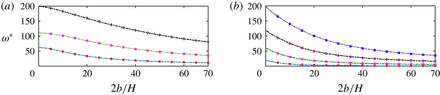
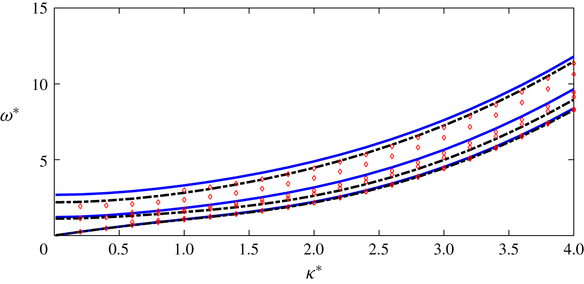
 $N=400$. Figure 2 provides the comparison between the present results with those by Bauer (Reference Bauer1993) for verification, in which
 $$\begin{eqnarray}\unicode[STIX]{x1D714}^{\ast }=\unicode[STIX]{x1D714}(2b)^{2}\sqrt{\unicode[STIX]{x1D70C}_{i}h_{i}/L};\quad \unicode[STIX]{x1D6FC}=\frac{\unicode[STIX]{x1D70C}g(2b)^{4}}{L};\quad \unicode[STIX]{x1D707}^{\ast }=\frac{\unicode[STIX]{x1D70C}_{i}h_{i}}{\unicode[STIX]{x1D70C}H}.\end{eqnarray}$$
We find that the results are in an excellent agreement.
Comparison of the first three and four natural frequencies respectively for clamped–clamped edge and clamped–free edge. (a) Clamped–clamped edge:  $\unicode[STIX]{x1D6FC}=100$,
 $\unicode[STIX]{x1D707}^{\ast }=10$, (b) clamped–free edge:
 $\unicode[STIX]{x1D6FC}=10,\unicode[STIX]{x1D707}^{\ast }=1$ (dotted-dashed lines: Bauer (Reference Bauer1993); markers: present results).

4.2 Dispersion relations
In the following calculations, the typical values for parameters are chosen as below:
 $$\begin{eqnarray}\left.\begin{array}{@{}c@{}}\unicode[STIX]{x1D70C}=1000~\text{kg}~\text{m}^{-3},\quad \unicode[STIX]{x1D70C}_{i}=917~\text{kg}~\text{m}^{-3},\quad E=4.2\times 10^{9}~\text{N}~\text{m}^{-2},\\ \unicode[STIX]{x1D708}=0.3,\quad g=9.81~\text{m}~\text{s}^{-2}.\end{array}\right\}\end{eqnarray}$$
Other parameters are chosen as  $h_{i}=0.1~\text{m}$,
 $H=5~\text{m}$ and
 $b=10~\text{m}$. The non-dimensionalization for the variables denoted by an asterisk is based on
 $g$,
 $\unicode[STIX]{x1D70C}$ and
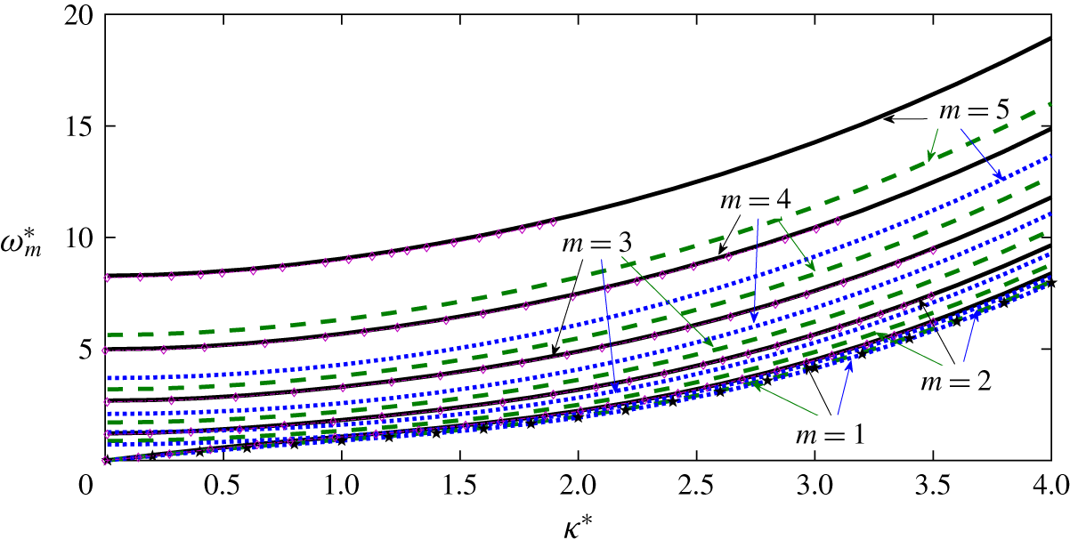
 $H$. In figure 3, we display the curves of the dispersion relationship for the first five wave frequencies varying with wavenumber
 $\unicode[STIX]{x1D705}^{\ast }$, corresponding to different edge conditions. From the figure, we can see that the results for clamped–clamped edges are in good agreement with those of Korobkin et al. (Reference Korobkin, Khabakhpasheva and Papin2014). We find that the first natural frequencies,
 $\unicode[STIX]{x1D714}_{1}^{\ast }$ corresponding to different edge conditions, are very close to each other. The difference in
 $\unicode[STIX]{x1D714}_{m}^{\ast }$ becomes significant as
 $m$ increases. Overall, at a given
 $\unicode[STIX]{x1D705}^{\ast }$, the clamped–clamped edge corresponds to the largest
 $\unicode[STIX]{x1D714}_{m}^{\ast }$, and the free–free edge to the smallest.
Dispersion relations at  $b^{\ast }=b/H=2$. Results for clamped–clamped, clamped–free and free–free edges are shown by solid, dashed and dotted lines, respectively. Results for
 $b=+\infty$ are shown as pentagram markers, and results from Korobkin et al. (Reference Korobkin, Khabakhpasheva and Papin2014) for clamped–clamped edge are converted to be non-dimensional and shown as diamond marks.

The results for an unbounded ocean or  $b=+\infty$ as
 $\unicode[STIX]{x1D714}^{\ast }=((1+L^{\ast }{\unicode[STIX]{x1D705}^{\ast }}^{4})/(\unicode[STIX]{x1D70C}_{i}^{\ast }h_{i}^{\ast }+1/(\unicode[STIX]{x1D705}^{\ast }\tanh \unicode[STIX]{x1D705}^{\ast })))^{1/2}$ are also provided for comparison. These has only one
 $\unicode[STIX]{x1D714}$ for each
 $\unicode[STIX]{x1D705}$ and the wave in this case will propagate only in the
 $x$ direction. For the free surface flow or
 $h=0$ in the channel, each
 $\unicode[STIX]{x1D714}_{m}$ corresponds to each transverse wave or each term of
 $a_{n}$ in (2.11) is fully independent, and a true one-dimensional wave is possible. However, in the ice-covered channel, the edge conditions in (2.21)–(2.23) make a single transverse wave impossible and they are all coupled. For a given
 $b$, the results for the free–free edge condition are closer to those of the unbounded case than the other two edge conditions. This can be expected as there is no connection between the ice and the walls in such a case.
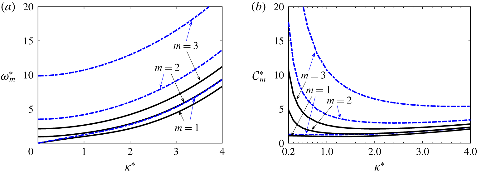
When simply supported edge conditions are assumed at both channel banks, the corresponding results are shown in figure 4. To investigate the influence of channel width on the dispersion relations, a narrower channel width, or  $b^{\ast }=1$, is chosen for comparison. From figure 4(a), we can find that the corresponding natural frequencies
 $\unicode[STIX]{x1D714}_{m}^{\ast }$ for each
 $\unicode[STIX]{x1D705}^{\ast }$ will increase when the channel width decreases. The wave celerity can be written as
 ${\mathcal{C}}_{m}^{\ast }=\unicode[STIX]{x1D714}_{m}^{\ast }/\unicode[STIX]{x1D705}^{\ast }$, which indicates that, for each
 $m$,
 ${\mathcal{C}}_{m}^{\ast }$ would be larger in a narrower channel than in a wider channel, as shown in figure 4(b). It is also worth noting that as we seek the solution of progressive waves in the form of (2.6), therefore the wavenumber
 $\unicode[STIX]{x1D705}^{\ast }$ does not vary across the channel.
(a) Dispersion relations and (b) wave celerity for both simply supported edge conditions at the channel banks. Dashed-dotted lines for  $b^{\ast }=1$ and solid lines for
 $b^{\ast }=2$.

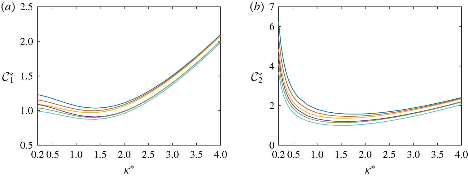
For other combinations of edge constraints at the banks, the dispersion relations can be obtained in a similar way. For the above three types of edge constraint, the number of combinations can be up to six. In the above analysis, we have mentioned four of them. It is interesting to further investigate all these edge constraints and their effect on the wave propagation, such as the wave celerity  ${\mathcal{C}}_{m}^{\ast }$. From figure 5, we can find that, at a given wavenumber, for different edge constraints, the corresponding wave celerity is decreasing in the following sequence: clamped–clamped, clamped–simply supported, simply supported–simply supported, clamped–free, simply supported–free and free–free.
Wave celerity  ${\mathcal{C}}_{m}^{\ast }\,(m=1,2)$ at
 $b^{\ast }=2$ corresponding to various edge constraints. For each
 $\unicode[STIX]{x1D705}^{\ast }$, the curves from above to below are respectively: clamped–clamped, clamped–simply supported, simply supported–simply supported, clamped–free, simply supported–free and free–free.

For the ice sheet with a longitudinal straight-line crack, the solution procedure in § 3 can be adopted. The influence of the crack on the dispersion relations is investigated by setting the crack at different positions. From figure 6, we can observe that the first natural frequency of the system with the crack at the centre, or  $l=0$, is very close to that of the continuous ice. The differences become much more obvious for the second and third natural frequencies, which indicates that the crack has a greater effect on larger frequencies. We can also observe that, when the crack is away from the channel centre, some natural frequencies are still around the results of a central crack. However, more natural frequencies may be found between these values for a certain
 $\unicode[STIX]{x1D705}^{\ast }$.
Dispersion relations at  $b^{\ast }=2$. Results for clamped–clamped edge at banks but a crack at
 $l^{\ast }=0,-0.25b^{\ast }$. Solid lines: continuous case; dashed-dotted lines: crack at
 $l^{\ast }=0$; diamonds: crack at
 $l^{\ast }=-0.25b^{\ast }$.

When the crack is at the centre of the ice sheet, the problem is symmetric if the edge conditions on both banks are the same. In such a case, it is expected that the ice deflections on two sides of the central crack can be either symmetric or anti-symmetric. Based on the kinematic equation, the corresponding flow field can be either symmetric or anti-symmetric with respect to the central plane of the channel. For the symmetric case, the Neumann boundary condition  $\unicode[STIX]{x2202}\unicode[STIX]{x1D719}/\unicode[STIX]{x2202}x=0$ can be imposed at the central plane. Therefore, the central plane can be seen as a rigid surface, and the central crack case is identical to the case of continuous ice with a clamped–free edge in a channel with a width of
 $b$. For the anti-symmetric case, the Dirichlet boundary condition should be imposed, or
 $\unicode[STIX]{x1D719}=0$, at the central plane. We further investigate the natural frequencies at a given wavenumber for Case 1: central crack and clamped–clamped edge at banks of a channel with a width of
 $2b$ and Case 2: continuous ice sheet with clamped–free edge at the banks of a channel with a width of
 $b$. By denoting the natural frequencies of Case 1 and Case 2 as respectively
 $\unicode[STIX]{x1D714}_{m}$ and
 $\widetilde{\unicode[STIX]{x1D714}}_{m}\,(m=1,2,3\ldots )$, we find that
 $\unicode[STIX]{x1D714}_{2m-1}=\widetilde{\unicode[STIX]{x1D714}}_{m}$, which indicates that in the central crack case (Case 1) the natural frequencies of odd numbers
 $\unicode[STIX]{x1D714}_{2m-1}\,(m=1,2,3\ldots )$ correspond to the symmetric situations while
 $\unicode[STIX]{x1D714}_{2m}\,(m=1,2,3\ldots )$ correspond to the anti-symmetric situations. The corresponding discussion on the deflection of ice sheet or wave profiles can be found in § 4.3. When the crack is away from the centre of the channel, the problem becomes asymmetric in geometry. In such a case, it does not correspond to symmetric or anti-symmetric situations and the flows on both sides of crack become more complex. As shown in figure 6, more natural frequencies appear in off-centre crack cases due to the asymmetry of the problem.
4.3 Wave profiles
For a specific pair of  $\unicode[STIX]{x1D705}^{\ast }$ and
 $\unicode[STIX]{x1D714}_{m}^{\ast }$ in the dispersion relation curve in figure 3, once one of the non-zero non-dimensional coefficients
 $c_{i}^{\ast }$ is prescribed, the others can be calculated through (2.25). The corresponding wave profiles can then be further obtained. It should be noted that the amplitude of the wave profile is proportional to
 $c_{i}^{\ast }$, and therefore choosing a different value for
 $c_{i}^{\ast }$ will not change the shape of the wave profiles. For a given real
 $c_{i}^{\ast }$, we can obtain other real coefficients from (2.25). From (2.12),
 $W(y)$ and its derivatives are all real. For the case with a clamped edge at
 $y^{\ast }=-b^{\ast }$, we have
 $c_{1}^{\ast }=0$ and therefore prescribe
 $c_{3}^{\ast }=1$; while for the case with a free edge at
 $y^{\ast }=-b^{\ast }$,
 $c_{1}^{\ast }=1$ is chosen.
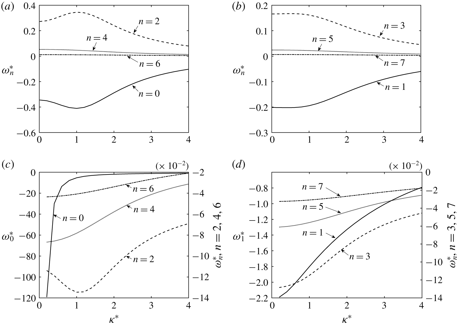
Amplitudes of transverse wave components for the first two natural frequencies  $\unicode[STIX]{x1D714}_{m}^{\ast }$ at
 $b^{\ast }=2$. (a) Clamped–clamped edge:
 $m=1\,(c_{3}^{\ast }=1)$; (b) clamped–clamped edge:
 $m=2\,(c_{3}^{\ast }=1)$; (c) free–free edge:
 $m=1\,(c_{1}^{\ast }=1)$; (d) free–free edge:
 $m=2\,(c_{1}^{\ast }=1)$.

 $$\begin{eqnarray}W(y)=\mathop{\sum }_{n=0}^{\infty }w_{n}\cos \unicode[STIX]{x1D70E}_{n}(y+b),\quad -b\leqslant y\leqslant b.\end{eqnarray}$$
We plot  $w_{n}^{\ast }=b_{n}^{\ast }k_{n}^{\ast }\sinh k_{n}^{\ast }$ for the first two
 $\unicode[STIX]{x1D714}_{m}^{\ast }$ to show the contribution of each term in the series to the wave profile in figure 7 for two cases without a crack. From the figure, we find that the first natural frequency (
 $m=1$) corresponds to symmetric modes, as only the terms with even
 $n$ are non-zero. The second natural frequency (
 $m=2$) corresponds to anti-symmetric modes, as only the terms with odd
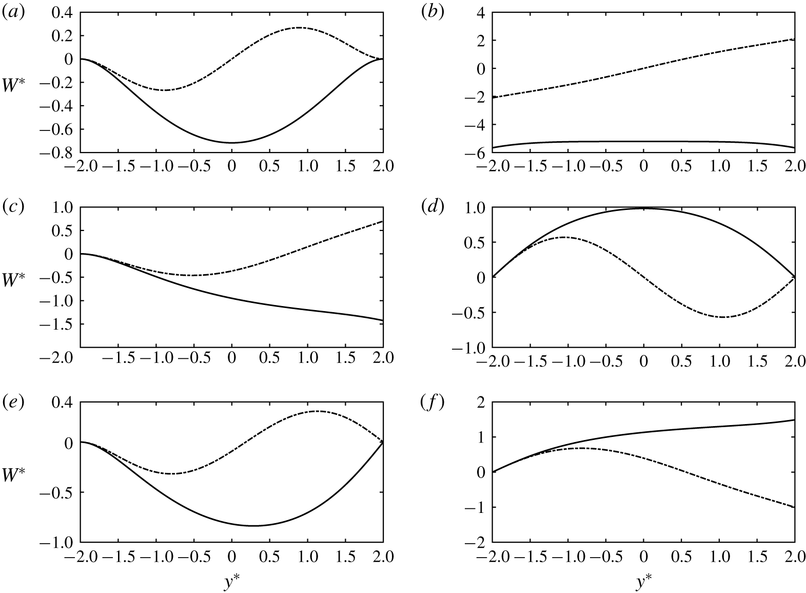
 $n$ are non-zero. In figure 8, we display the wave profiles corresponding to the first two natural frequencies for different edge conditions at the same wavenumber. For cases with the same edge conditions on both banks, the deflection curves are respectively symmetric and anti-symmetric with respect to
 $y^{\ast }=0$ at the first and second natural frequencies, which can be observed in figure 8(a,b,d). While for cases where different edge constraints are imposed at the two banks, the symmetry and anti-symmetry are no longer shown in the deflection curves, such as in figure 8(c,e,f). For the clamped–free edge case, the deflection at the left side bank is always zero due to the clamped edge conditions while it is free at the right side bank.
Wave profiles of hydroelastic waves in the channel at  $\unicode[STIX]{x1D705}^{\ast }=1$ and
 $b^{\ast }=2$. (a) Clamped–clamped edge
 $(c_{3}^{\ast }=1)$, (b) free–free edge
 $(c_{1}^{\ast }=1)$, (c) clamped–free edge
 $(c_{3}^{\ast }=1)$, (d) both simply supported edges
 $(c_{1}^{\ast }=1)$, (e) clamped–simply supported edge
 $(c_{3}^{\ast }=1)$, (f) simply supported–free edge
 $(c_{1}^{\ast }=1)$. Solid lines for the first natural frequency and dashed-dotted lines for the second natural frequency.

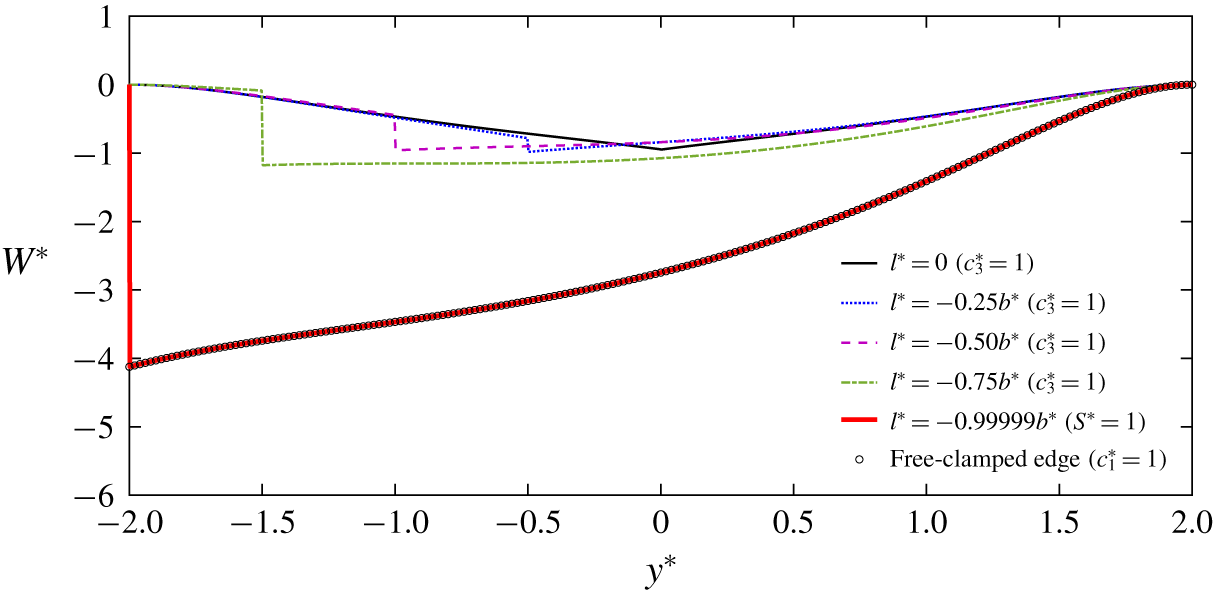
Similarly, the wave profiles are also displayed for the cases of clamped–clamped edge at the channel banks and a crack at various positions for their first natural frequencies. The jumps of deflection and slope at the crack are displayed in figure 9 for a given unit  $c_{3}^{\ast }$. From the figure, we observe that changing the position of the crack has an obvious influence on the deflection and slope of the ice sheet. It is also worth pointing out that for the crack case we retain the expression of the deflection in the form of (2.12). The
 $c_{i}\,(i=0\sim 3)$ may still be related to the edge conditions. However, they are no longer the same as those without crack as they will be influenced by
 $S$ and
 $D$. Specifically, for the clamped–clamped case, when the crack indefinitely approaches the left bank, or
 $l^{\ast }\rightarrow -b^{\ast }$, the slope at left side of the crack is zero based on the clamped edge conditions or
 $W_{1}^{\prime }(-b)=0$. Therefore, based on the definition of
 $S$, which is the jump of the slopes at the crack,
 $S$ should refer to the slope at the right side of the crack, or
 $W_{2}^{\prime }(-b)$. In such a case when
 $l^{\ast }\rightarrow -b^{\ast }$, the ice edge at the wall has become a free edge. Then the result is expected to be the same as the free–clamped case without a crack. Thus, we take
 $l^{\ast }=-0.99999b^{\ast }$ and give a unit
 $S^{\ast }$ in the crack case, and we also give a unit slope
 $c_{1}^{\ast }$ at
 $y=-b$ for the free–clamped case. The numerical results in figure 9 show that there is no difference between the ice sheet deflections.
Wave profiles of hydroelastic waves in the channel with clamped–clamped edge at channel banks and a crack at different positions for the first natural frequency at  $b^{\ast }=2,\unicode[STIX]{x1D705}^{\ast }=1$. Results for continuous ice sheet of free–clamped edge at
 $c_{1}^{\ast }=1$ are shown as circle markers.

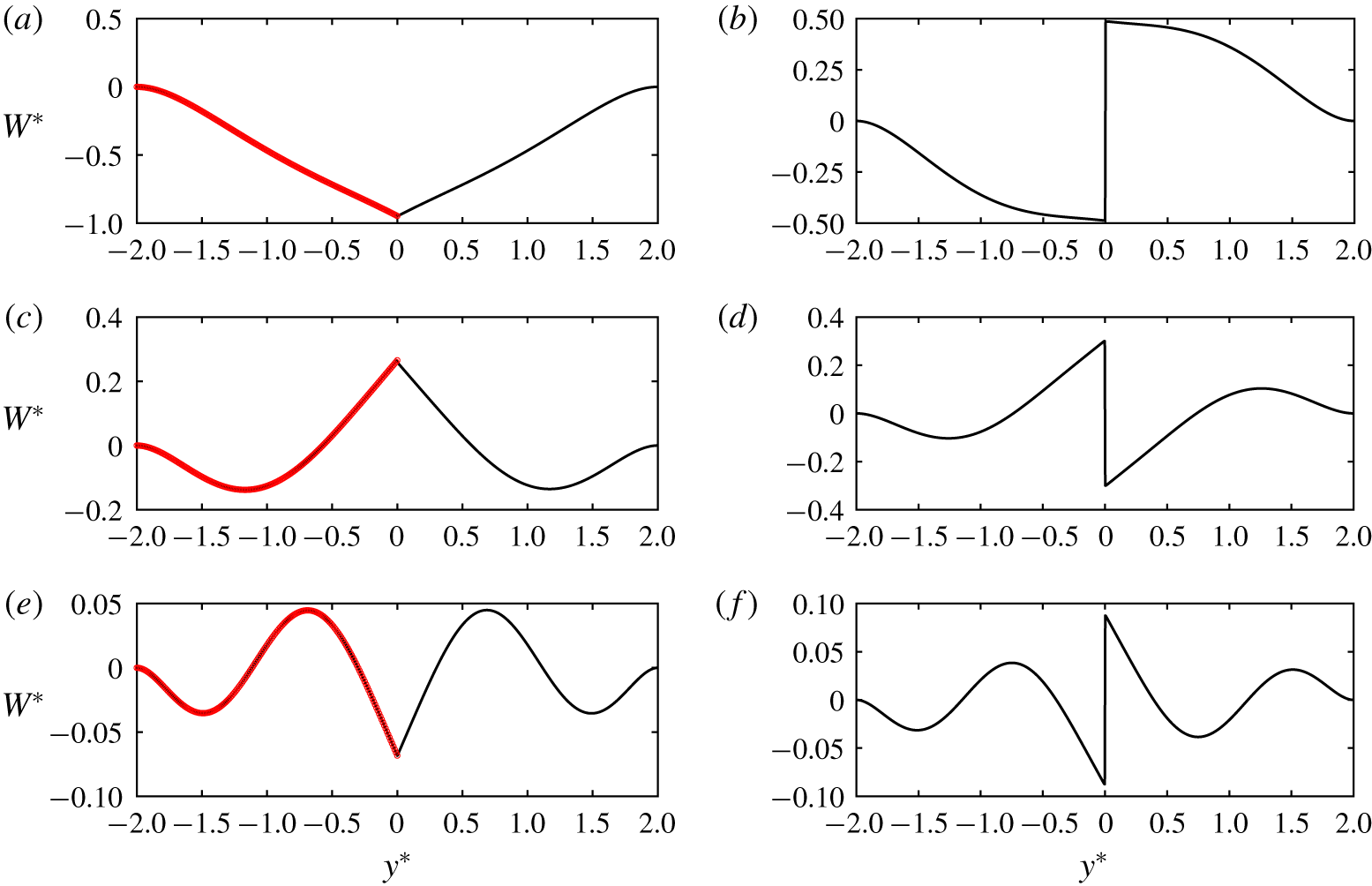
Further to the discussion on the central crack case in § 4.2, the wave deflection across the channel for the central crack case (Case 1) for the first six natural frequencies is displayed in figure 10. For the odd number natural frequencies, the corresponding wave profiles for the continuous ice with clamped–free edge at the banks of the channel with a width of  $b$ (Case 2) are also displayed for comparison. Consistent with the discussion in § 4.2, the wave profiles of the central crack case for the natural frequencies of odd
 $m$ are symmetric to the central plane, while for the natural frequencies of even
 $m$, the corresponding wave profiles are anti-symmetric to the central plane. Besides, for odd
 $m$, the deflection curves of Case 1 and Case 2 are the same, which in turn further verifies the effectiveness and rationality of the solution procedure in § 3.
Wave deflection of hydroelastic waves in the channel with clamped–clamped edge at channel banks and a central crack for the first six natural frequencies  $\unicode[STIX]{x1D714}_{m}^{\ast }\,(m=1\sim 6)$ at
 $b^{\ast }=2$,
 $\unicode[STIX]{x1D705}^{\ast }=1$ and
 $c_{3}^{\ast }=1$. From left to right and from top to bottom,
 $m=1,2,3,4,5$ and
 $6$. Results for a continuous ice sheet of clamped–free edge in a channel for the first three natural frequencies
 $\widetilde{\unicode[STIX]{x1D714}}_{(m+1)/2}\,(m=1,3,5)$ at
 $b^{\ast }=1$,
 $\unicode[STIX]{x1D705}^{\ast }=1$,
 $c_{3}^{\ast }=1$ are shown as circle markers for comparison (the abscissa has been translated from
 $[-1,1]$ to
 $[-2,0]$ for comparison).

4.4 Strain in the ice
The strain of the ice is an important physical parameter which is associated with its fracture and breakup when it becomes excessive. Based on the usual definition of principal stress (strain) (Timoshenko & Woinowsky-Krieger Reference Timoshenko and Woinowsky-Krieger1959), the principal strain  $\unicode[STIX]{x1D706}$ can be obtained as the eigenvalues of the strain tensor matrix
 $\unicode[STIX]{x1D700}=-(h_{i}/2)\big(\!\begin{smallmatrix}w_{xx} & w_{xy}\\ w_{xy} & w_{yy}\\ \end{smallmatrix}\!\big)$, or the solution of
 $\det [\unicode[STIX]{x1D700}-\unicode[STIX]{x1D706}I]=0$. Then, we can simplify the principal strain as
 $$\begin{eqnarray}\displaystyle \unicode[STIX]{x1D706}_{1,2} & = & \displaystyle \frac{h_{i}}{4}\left\{[\unicode[STIX]{x1D705}^{2}W(y)-W^{\prime \prime }(y)]\cos (\unicode[STIX]{x1D705}x-\unicode[STIX]{x1D714}t)\right.\nonumber\\ \displaystyle & & \displaystyle \pm \left.\sqrt{[\unicode[STIX]{x1D705}^{2}W(y)+W^{\prime \prime }(y)]^{2}\cos ^{2}(\unicode[STIX]{x1D705}x-\unicode[STIX]{x1D714}t)+[2\unicode[STIX]{x1D705}W^{\prime }(y)]^{2}\sin ^{2}(\unicode[STIX]{x1D705}x-\unicode[STIX]{x1D714}t)}\right\}.\end{eqnarray}$$
Here,  $\unicode[STIX]{x1D706}_{1,2}$ is a function of
 $\unicode[STIX]{x1D6FD}=\unicode[STIX]{x1D705}x-\unicode[STIX]{x1D714}t$. It has extremes
 $\unicode[STIX]{x1D706}_{M}^{(i)}$,
 $i=1\sim 4$, at
 $\unicode[STIX]{x2202}\unicode[STIX]{x1D706}_{1,2}/\unicode[STIX]{x2202}\unicode[STIX]{x1D6FD}=0$. Thus, the maximum principal strain can be obtained from
 $\unicode[STIX]{x1D706}_{M}(y)=\max _{i=1\sim 4}\{\unicode[STIX]{x1D706}_{M}^{(i)}\}$, where
 $$\begin{eqnarray}\left.\begin{array}{@{}c@{}}\displaystyle \unicode[STIX]{x1D706}_{M}^{(1)}=\frac{h_{i}}{2}|W^{\prime \prime }(y)|,\quad \unicode[STIX]{x1D706}_{M}^{(2)}=\frac{h_{i}}{2}\unicode[STIX]{x1D705}^{2}|W(y)|,\\ \displaystyle \unicode[STIX]{x1D706}_{M}^{(3)}=\frac{h_{i}}{2}|(4\unicode[STIX]{x1D705}^{2}WW^{\prime \prime }-4\unicode[STIX]{x1D705}^{2}{W^{\prime }}^{2})/\unicode[STIX]{x1D6E4}|,\\ \displaystyle \unicode[STIX]{x1D706}_{M}^{(4)}=\frac{h_{i}}{2}|(-2\unicode[STIX]{x1D705}^{4}W^{2}-2{W^{\prime \prime }}^{2}+4\unicode[STIX]{x1D705}^{2}{W^{\prime }}^{2})/\unicode[STIX]{x1D6E4}|,\end{array}\right\}\end{eqnarray}$$
and
 $$\begin{eqnarray}\unicode[STIX]{x1D6E4}=2(\unicode[STIX]{x1D705}^{2}W-W^{\prime \prime })\sqrt{1+\frac{[4\unicode[STIX]{x1D705}^{2}{W^{\prime }}^{2}-(\unicode[STIX]{x1D705}^{2}W+W^{\prime \prime })^{2}]^{2}-(\unicode[STIX]{x1D705}^{2}W+W^{\prime \prime })^{2}(\unicode[STIX]{x1D705}^{2}W-W^{\prime \prime })^{2}}{4\unicode[STIX]{x1D705}^{2}{W^{\prime }}^{2}[\unicode[STIX]{x1D705}^{2}W-W^{\prime \prime }]^{2}}}.\end{eqnarray}$$
It should be noted that  $\unicode[STIX]{x1D706}_{M}^{(3)}$ and
 $\unicode[STIX]{x1D706}_{M}^{(4)}$ can exist only when
 $[4\unicode[STIX]{x1D705}^{2}{W^{\prime }}^{2}-(\unicode[STIX]{x1D705}^{2}W+W^{\prime \prime })^{2}]^{2}\geqslant (\unicode[STIX]{x1D705}^{4}W^{2}-{W^{\prime \prime }}^{2})^{2}$. In figure 11,
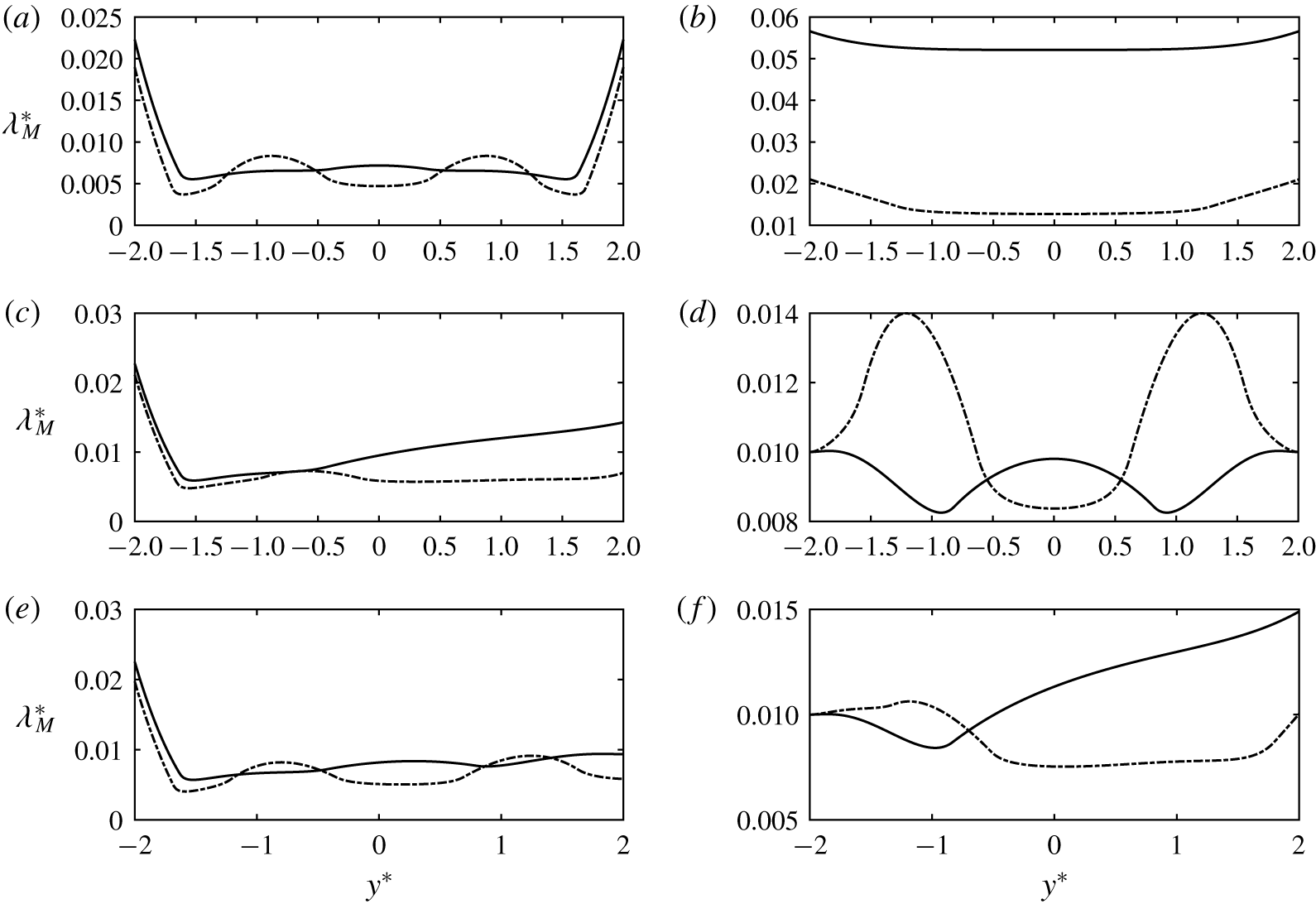
 $\unicode[STIX]{x1D706}_{M}(y)$ is displayed for the waves corresponding to the first two natural frequencies for the clamped–clamped, free–free, clamped–free, both simply supported, clamped–simply supported and simply supported–free edges. It can be seen that for the clamped–clamped edge case, the maximum principal strain can be much larger at the walls than at other places, which indicates that the fracture or breakup may be more likely to occur along the channel banks. When the constraint at the right side bank becomes a free edge, or in the clamped–free edge case, the peak of the maximum principal strain is still located at the clamped end. For the free–free edge case, although the peaks are still located at both banks, the curves become much flatter across the channel than those of the clamped–clamped case. However, the results might be different in the both simply supported edge case, as observed in figure 11(d), where the maxima of the maximum principal strain occur at a distance from the edges. In such a case, cracks might be more likely to occur at a distance away from the channel banks. We may further consider the curves in figure 11(a,d) from the expressions of
 $\unicode[STIX]{x1D706}_{M}^{(i)}$ to investigate their difference. At banks of clamped edges, we can have
 $\unicode[STIX]{x1D706}_{M}^{(2)}(\pm b)=0$ due to
 $W(\pm b)=W^{\prime }(\pm b)=0$. We may also find that the corresponding
 $\unicode[STIX]{x1D706}_{M}^{(3)}(\pm b)$ and
 $\unicode[STIX]{x1D706}_{M}^{(4)}(\pm b)$ equal to zero. Therefore, we can have
 $\unicode[STIX]{x1D706}_{M}(\pm b)=\unicode[STIX]{x1D706}_{M}^{(1)}(\pm b)=h_{i}|W^{\prime \prime }(\pm b)|/2$, which is related to the ice thickness and the second derivatives of the deflection. While at the banks with simply supported edges, we have
 $W(\pm b)=W^{\prime \prime }(\pm b)=0$, so we can have
 $\unicode[STIX]{x1D706}_{M}^{(1)}(\pm b)=\unicode[STIX]{x1D706}_{M}^{(2)}(\pm b)=0$. The results for
 $\unicode[STIX]{x1D706}_{M}^{(3)}$ and
 $\unicode[STIX]{x1D706}_{M}^{(4)}$ at
 $y=\pm b$ equal to
 $h_{i}\unicode[STIX]{x1D705}|W^{\prime }|/2$, which indicates that the maximum principal strain at the banks is related to the ice thickness, wavenumber and the slope at the edge. For figure 11(d), the peaks for the first natural frequency are quite close to the channel banks, and these values are obtained from
 $\unicode[STIX]{x1D706}_{M}^{(3)}$, which are slightly larger than those at the channel banks. While for the second natural frequency, the peaks are located around one/three quarter(s) of the channel and can be much larger than those at the channel banks, which are obtained from
 $\unicode[STIX]{x1D706}_{M}^{(1)}$.
The distribution of the maximum principal strains across the channel for the (a) clamped–clamped  $(c_{3}^{\ast }=1)$, (b) free–free
 $(c_{1}^{\ast }=1)$, (c) clamped–free
 $(c_{3}^{\ast }=1)$, (d) both simply supported
 $(c_{1}^{\ast }=1)$, (e) clamped–simply supported
 $(c_{3}^{\ast }=1)$, (f) simply supported–free
 $(c_{1}^{\ast }=1)$ for the first and second natural frequencies at
 $b^{\ast }=2$,
 $\unicode[STIX]{x1D705}^{\ast }=1$. Solid lines: first natural frequency, dashed-dotted lines: second natural frequency.

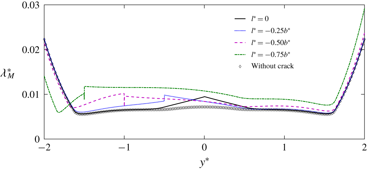
The effect of a crack on the distribution of the maximum principal strains across the ice sheet is also studied. It is worth noting that, similar to the procedure in § 3, non-convergent terms associated with  $\unicode[STIX]{x1D6FF}(y-l)$ and its derivatives need to be removed from the infinite series in the expressions of
 $W^{\prime }$ and
 $W^{\prime \prime }$ when calculating the maximum principal strain across the channel. In figure 12, we display the maximum principal strains across the channel for the clamped–clamped case with a crack at various positions for their first natural frequencies. From the figure, we observe that with the crack moving from the centre to the left bank, the maximum principal strains at the right bank keep increasing while those at the left bank keep decreasing, which indicates that when there has already been a longitudinal crack in the ice sheet near one bank, the connection between the ice sheet and the opposite bank might be more likely to be damaged as well.
The distribution of the maximum principal strains across the channel for the clamped–clamped case with a crack at various positions for their first natural frequencies at  $b^{\ast }=2,\unicode[STIX]{x1D705}^{\ast }=1,c_{3}^{\ast }=1$. The curve for the continuous ice sheet with clamped–clamped edge at the channel banks is displayed with diamond markers for comparison.

5 Conclusions
We have investigated the behaviour of hydroelastic waves in a channel covered by an ice sheet based on the linearized velocity potential and the thin elastic plate model. An efficient analytical solution procedure is developed, which allows the solution for an ice sheet with various edge conditions and with a crack to be obtained easily. The effectiveness of the solution procedure has been verified by comparison with the results of a two-dimensional sloshing tank and with the existing result for an ice sheet in a channel with clamped edges.
From the results, we observe that for a given wavenumber, the wave celerity is largest when both edges of ice sheet are clamped into the channel banks. The celerity decreases when its two edge constraints change from clamped to simply supported and further decreases when they change to free. For the same edge constraints at the two banks, the wave profiles across the channel can be either symmetric or anti-symmetric with respect to the central plane of the channel, which corresponds to natural frequencies of odd and even numbers, respectively. While for different edge constraints at the channel banks, the wave profiles become asymmetric. We also observe that the local peaks of the maximum principal strain in the ice across the channel usually occur at the clamped or free ends at the first two natural frequencies. However, it is different for a simply supported edge, where the local peaks of the maximum principal strain are usually at some distance from the edges.
The effect of position of the crack on the wave propagation is investigated through the dispersion relations, wave profiles and strain distribution. It has been shown that when the crack of free edges indefinitely approaches one channel bank, the result tends to that of an ice sheet with a free end. Also, for an ice sheet with the same edge conditions at the channel banks and a central crack, due to the symmetry, the corresponding natural frequencies and the propagation features can be simply explained through symmetric and anti-symmetric cases, in which the Neumann and Dirichlet boundary conditions can be imposed on the central plane of the channel, respectively.
The procedure developed in this paper can be further extended to problems with multiple longitudinal cracks, where more complex interactions between water waves and ice cover are expected. Furthermore, cracks with other forms of edge constraints can be also investigated by this method. It is also worth noting that the effect of the wind pressure on the ice sheet can be further incorporated into the present work. In such a case, an external pressure term can be added into the dynamic boundary condition of the ice sheet, which requires a particular solution to be added to the general solution in this paper.
Acknowledgements
The first author is sponsored by a joint scholarship from University College London and China Scholarships Council, to which he is most grateful. This work is also supported by the Lloyd’s Register Foundation. The LRF helps protect life and property by supporting engineering-related education, public engagement, and the application of research.
Declaration of interests
The authors report no conflict of interest.
Appendix A. Coefficient matrix  $\unicode[STIX]{x1D608}_{ij}$ of clamped–clamped edge with and without a crack

From the clamped condition at the left bank, or  $W^{\prime }(-b)=0$, we have
 $c_{1}=0$ and therefore the general
 $6\times 6$ matrix
 $\boldsymbol{A}$ for the case with a crack can be reduced to
 $5\times 5$. For
 $\boldsymbol{C}=[c_{0};c_{2};c_{3};D;S]$, from (2.24) and (3.12), the coefficients
 $\unicode[STIX]{x1D608}_{ij}$ can be written as
 $$\begin{eqnarray}A_{1j}=\unicode[STIX]{x1D6FF}_{1j}\left(1+\mathop{\sum }_{n=1}^{\infty }\frac{\unicode[STIX]{x1D6FC}_{n0}}{\unicode[STIX]{x1D70E}_{n}^{4}}\right)+(1-\unicode[STIX]{x1D6FF}_{1j})\mathop{\sum }_{n=1}^{\infty }\frac{\unicode[STIX]{x1D6FC}_{nj}}{\unicode[STIX]{x1D70E}_{n}^{4}};\end{eqnarray}$$
 $$\begin{eqnarray}\displaystyle A_{2j} & = & \displaystyle \unicode[STIX]{x1D6FF}_{1j}\left(1+\frac{2b^{4}}{3}\unicode[STIX]{x1D6FC}_{00}+\mathop{\sum }_{n=1}^{\infty }\frac{\cos n\unicode[STIX]{x03C0}}{\unicode[STIX]{x1D70E}_{n}^{4}}\unicode[STIX]{x1D6FC}_{n0}\right)+4\unicode[STIX]{x1D6FF}_{2j}b^{2}+8\unicode[STIX]{x1D6FF}_{3j}b^{3}\nonumber\\ \displaystyle & & \displaystyle +\,(1-\unicode[STIX]{x1D6FF}_{1j})\left(\frac{2b^{4}}{3}\unicode[STIX]{x1D6FC}_{0j}+\mathop{\sum }_{n=1}^{\infty }\frac{\cos n\unicode[STIX]{x03C0}}{\unicode[STIX]{x1D70E}_{n}^{4}}\unicode[STIX]{x1D6FC}_{nj}\right);\end{eqnarray}$$
 $$\begin{eqnarray}A_{3j}=\unicode[STIX]{x1D6FF}_{1j}\left(\frac{4b^{3}}{3}\unicode[STIX]{x1D6FC}_{00}\right)+4\unicode[STIX]{x1D6FF}_{2j}b+12\unicode[STIX]{x1D6FF}_{3j}b^{2}+(1-\unicode[STIX]{x1D6FF}_{1j})\frac{4b^{3}}{3}\unicode[STIX]{x1D6FC}_{0j};\end{eqnarray}$$
 $$\begin{eqnarray}\displaystyle A_{4j} & = & \displaystyle \unicode[STIX]{x1D6FF}_{1j}\left[\frac{(l+b)^{2}}{2}\unicode[STIX]{x1D6FC}_{00}-\mathop{\sum }_{n=1}^{\infty }\frac{\cos \unicode[STIX]{x1D70E}_{n}(l+b)}{\unicode[STIX]{x1D70E}_{n}^{2}}\unicode[STIX]{x1D6FC}_{n0}\right.\nonumber\\ \displaystyle & & \displaystyle -\left.\unicode[STIX]{x1D708}\unicode[STIX]{x1D705}^{2}\left(1+\frac{(l+b)^{4}}{24}\unicode[STIX]{x1D6FC}_{00}+\mathop{\sum }_{n=1}^{\infty }\frac{\cos \unicode[STIX]{x1D70E}_{n}(l+b)}{\unicode[STIX]{x1D70E}_{n}^{4}}\unicode[STIX]{x1D6FC}_{n0}\right)\right]\nonumber\\ \displaystyle & & \displaystyle +\,\unicode[STIX]{x1D6FF}_{2j}[2-\unicode[STIX]{x1D708}\unicode[STIX]{x1D705}^{2}(l+b)^{2}]+\unicode[STIX]{x1D6FF}_{3j}[6(l+b)-\unicode[STIX]{x1D708}\unicode[STIX]{x1D705}^{2}(l+b)^{3}]\nonumber\\ \displaystyle & & \displaystyle +\,(1-\unicode[STIX]{x1D6FF}_{1j})\left[\frac{(l+b)^{2}}{2}\unicode[STIX]{x1D6FC}_{0j}-\mathop{\sum }_{n=1}^{\infty }\frac{\cos \unicode[STIX]{x1D70E}_{n}(l+b)}{\unicode[STIX]{x1D70E}_{n}^{2}}\unicode[STIX]{x1D6FC}_{nj}\right.\nonumber\\ \displaystyle & & \displaystyle -\left.\unicode[STIX]{x1D708}\unicode[STIX]{x1D705}^{2}\left(\frac{(l+b)^{4}}{24}\unicode[STIX]{x1D6FC}_{0j}+\mathop{\sum }_{n=1}^{\infty }\frac{\cos \unicode[STIX]{x1D70E}_{n}(l+b)}{\unicode[STIX]{x1D70E}_{n}^{4}}\unicode[STIX]{x1D6FC}_{nj}\right)\right];\end{eqnarray}$$
 $$\begin{eqnarray}\displaystyle A_{5j} & = & \displaystyle \unicode[STIX]{x1D6FF}_{1j}\left[(l+b)\unicode[STIX]{x1D6FC}_{00}+\mathop{\sum }_{n=1}^{\infty }\frac{\sin \unicode[STIX]{x1D70E}_{n}(l+b)}{\unicode[STIX]{x1D70E}_{n}}\unicode[STIX]{x1D6FC}_{n0}\right.\nonumber\\ \displaystyle & & \displaystyle -\left.(2-\unicode[STIX]{x1D708})\unicode[STIX]{x1D705}^{2}\left(\frac{(l+b)^{3}}{6}\unicode[STIX]{x1D6FC}_{00}-\mathop{\sum }_{n=1}^{\infty }\frac{\sin \unicode[STIX]{x1D70E}_{n}(l+b)}{\unicode[STIX]{x1D70E}_{n}^{3}}\unicode[STIX]{x1D6FC}_{n0}\right)\right]\nonumber\\ \displaystyle & & \displaystyle -\,2\unicode[STIX]{x1D6FF}_{2j}(l+b)(2-\unicode[STIX]{x1D708})\unicode[STIX]{x1D705}^{2}+\unicode[STIX]{x1D6FF}_{3j}[6-3(2-\unicode[STIX]{x1D708})\unicode[STIX]{x1D705}^{2}(l+b)^{2}]\nonumber\\ \displaystyle & & \displaystyle +\,(1-\unicode[STIX]{x1D6FF}_{1j})\left[(l+b)\unicode[STIX]{x1D6FC}_{0j}+\mathop{\sum }_{n=1}^{\infty }\frac{\sin \unicode[STIX]{x1D70E}_{n}(l+b)}{\unicode[STIX]{x1D70E}_{n}}\unicode[STIX]{x1D6FC}_{nj}\right.\nonumber\\ \displaystyle & & \displaystyle -\left.(2-\unicode[STIX]{x1D708})\unicode[STIX]{x1D705}^{2}\left(\frac{(l+b)^{3}}{6}\unicode[STIX]{x1D6FC}_{0j}-\mathop{\sum }_{n=1}^{\infty }\frac{\sin \unicode[STIX]{x1D70E}_{n}(l+b)}{\unicode[STIX]{x1D70E}_{n}^{3}}\unicode[STIX]{x1D6FC}_{nj}\right)\right].\end{eqnarray}$$
We notice that non-convergent terms exist in the infinite series in  $A_{44}$,
 $A_{45}$,
 $A_{54}$ and
 $A_{55}$, which can be removed by using the Dirac delta function and its derivatives in (3.6). Subsequently, these equations become
 $$\begin{eqnarray}\displaystyle A_{44}^{\ast } & = & \displaystyle \left(\frac{(l+b)^{2}}{2}-\unicode[STIX]{x1D708}\unicode[STIX]{x1D705}^{2}\frac{(l+b)^{4}}{24}\right)\unicode[STIX]{x1D6FC}_{04}-\mathop{\sum }_{n=1}^{\infty }\frac{\unicode[STIX]{x1D70E}_{n}\cos \unicode[STIX]{x1D70E}_{n}(l+b)\sin \unicode[STIX]{x1D70E}_{n}(l+b)}{b}\nonumber\\ \displaystyle & & \displaystyle \times \,\left\{\frac{\displaystyle -(\unicode[STIX]{x1D70C}g-\unicode[STIX]{x1D714}^{2}\unicode[STIX]{x1D70C}_{i}h_{i}+L\unicode[STIX]{x1D705}^{4})+\frac{\unicode[STIX]{x1D70C}\unicode[STIX]{x1D714}^{2}\coth k_{n}H}{k_{n}}+\unicode[STIX]{x1D708}(2-\unicode[STIX]{x1D708})\unicode[STIX]{x1D705}^{4}L}{\displaystyle -\left[(\unicode[STIX]{x1D70C}g-\unicode[STIX]{x1D714}^{2}\unicode[STIX]{x1D70C}_{i}h_{i}+L\unicode[STIX]{x1D705}^{4})+2\unicode[STIX]{x1D705}^{2}L\unicode[STIX]{x1D70E}_{n}^{2}+L\unicode[STIX]{x1D70E}_{n}^{4}\right]+\frac{\unicode[STIX]{x1D70C}\unicode[STIX]{x1D714}^{2}\coth k_{n}H}{k_{n}}}\right\};\end{eqnarray}$$
 $$\begin{eqnarray}\displaystyle A_{45}^{\ast } & = & \displaystyle \left(\frac{(l+b)^{2}}{2}-\unicode[STIX]{x1D708}\unicode[STIX]{x1D705}^{2}\frac{(l+b)^{4}}{24}\right)\unicode[STIX]{x1D6FC}_{05}-\frac{1}{2b}\nonumber\\ \displaystyle & & \displaystyle -\,\mathop{\sum }_{n=1}^{\infty }\left\{\frac{\cos ^{2}\unicode[STIX]{x1D70E}_{n}(l+b)}{b}\right.\nonumber\\ \displaystyle & & \displaystyle \times \,\left[\frac{\displaystyle (2\unicode[STIX]{x1D708}-2)\unicode[STIX]{x1D705}^{2}L\unicode[STIX]{x1D70E}_{n}^{2}+\unicode[STIX]{x1D708}^{2}\unicode[STIX]{x1D705}^{4}L-(\unicode[STIX]{x1D70C}g-\unicode[STIX]{x1D714}^{2}\unicode[STIX]{x1D70C}_{i}h_{i}+L\unicode[STIX]{x1D705}^{4})+\frac{\unicode[STIX]{x1D70C}\unicode[STIX]{x1D714}^{2}\coth k_{n}H}{k_{n}}}{\displaystyle -\left[(\unicode[STIX]{x1D70C}g-\unicode[STIX]{x1D714}^{2}\unicode[STIX]{x1D70C}_{i}h_{i}+L\unicode[STIX]{x1D705}^{4})+2\unicode[STIX]{x1D705}^{2}L\unicode[STIX]{x1D70E}_{n}^{2}+L\unicode[STIX]{x1D70E}_{n}^{4}\right]+\frac{\unicode[STIX]{x1D70C}\unicode[STIX]{x1D714}^{2}\coth k_{n}H}{k_{n}}}\right]\nonumber\\ \displaystyle & & \displaystyle +\,\frac{\unicode[STIX]{x1D6FC}_{05}\cos \unicode[STIX]{x1D70E}_{n}(l+b)}{\unicode[STIX]{x1D6E5}_{n}}\left(\frac{1}{\unicode[STIX]{x1D70E}_{n}^{2}}+\frac{\unicode[STIX]{x1D708}\unicode[STIX]{x1D705}^{2}}{\unicode[STIX]{x1D70E}_{n}^{4}}\right)\left[\frac{(\unicode[STIX]{x1D70C}g-\unicode[STIX]{x1D714}^{2}\unicode[STIX]{x1D70C}_{i}h_{i}+L\unicode[STIX]{x1D705}^{4})d_{n}^{(4)}k_{n}\sinh k_{n}H}{24}\right.\nonumber\\ \displaystyle & & \displaystyle -\left.\left.\unicode[STIX]{x1D705}^{2}Ld_{n}^{(2)}k_{n}\sinh k_{n}H-\unicode[STIX]{x1D70C}\unicode[STIX]{x1D714}^{2}\frac{d_{n}^{(4)}}{24}\cosh k_{n}H\right]\right\};\end{eqnarray}$$
 $$\begin{eqnarray}\displaystyle A_{54}^{\ast } & = & \displaystyle \left((l+b)-(2-\unicode[STIX]{x1D708})\unicode[STIX]{x1D705}^{2}\frac{(l+b)^{3}}{6}\right)\unicode[STIX]{x1D6FC}_{04}\nonumber\\ \displaystyle & & \displaystyle +\,\mathop{\sum }_{n=1}^{\infty }\frac{\unicode[STIX]{x1D70E}_{n}^{2}\sin ^{2}\unicode[STIX]{x1D70E}_{n}(l+b)}{b}\nonumber\\ \displaystyle & & \displaystyle \times \,\left[\frac{\displaystyle -(\unicode[STIX]{x1D70C}g-\unicode[STIX]{x1D714}^{2}\unicode[STIX]{x1D70C}_{i}h_{i}+L\unicode[STIX]{x1D705}^{4})+\frac{\unicode[STIX]{x1D70C}\unicode[STIX]{x1D714}^{2}\coth k_{n}H}{k_{n}}}{\displaystyle -\left[(\unicode[STIX]{x1D70C}g-\unicode[STIX]{x1D714}^{2}\unicode[STIX]{x1D70C}_{i}h_{i}+L\unicode[STIX]{x1D705}^{4})+2\unicode[STIX]{x1D705}^{2}L\unicode[STIX]{x1D70E}_{n}^{2}+L\unicode[STIX]{x1D70E}_{n}^{4}\right]+\frac{\unicode[STIX]{x1D70C}\unicode[STIX]{x1D714}^{2}\coth k_{n}H}{k_{n}}}\right]\nonumber\\ \displaystyle & & \displaystyle +\,\mathop{\sum }_{n=1}^{\infty }\frac{\sin ^{2}\unicode[STIX]{x1D70E}_{n}(l+b)}{b}\nonumber\\ \displaystyle & & \displaystyle \times \,\left[\frac{\displaystyle (2\unicode[STIX]{x1D708}-2)\unicode[STIX]{x1D705}^{2}\left(\unicode[STIX]{x1D70C}g-\unicode[STIX]{x1D714}^{2}\unicode[STIX]{x1D70C}_{i}h_{i}+L\unicode[STIX]{x1D705}^{4}-\frac{\unicode[STIX]{x1D70C}\unicode[STIX]{x1D714}^{2}\coth k_{n}H}{k_{n}}\right)+\unicode[STIX]{x1D708}^{2}\unicode[STIX]{x1D705}^{4}L\unicode[STIX]{x1D70E}_{n}^{2}}{\displaystyle -\left[(\unicode[STIX]{x1D70C}g-\unicode[STIX]{x1D714}^{2}\unicode[STIX]{x1D70C}_{i}h_{i}+L\unicode[STIX]{x1D705}^{4})+2\unicode[STIX]{x1D705}^{2}L\unicode[STIX]{x1D70E}_{n}^{2}+L\unicode[STIX]{x1D70E}_{n}^{4}\right]+\frac{\unicode[STIX]{x1D70C}\unicode[STIX]{x1D714}^{2}\coth k_{n}H}{k_{n}}}\right];\qquad\end{eqnarray}$$
 $$\begin{eqnarray}\displaystyle A_{55}^{\ast } & = & \displaystyle \left((l+b)-(2-\unicode[STIX]{x1D708})\unicode[STIX]{x1D705}^{2}\frac{(l+b)^{3}}{6}\right)\unicode[STIX]{x1D6FC}_{05}+(2-\unicode[STIX]{x1D708})\unicode[STIX]{x1D705}^{2}\mathop{\sum }_{n=1}^{\infty }\frac{\sin \unicode[STIX]{x1D70E}_{n}(l+b)}{\unicode[STIX]{x1D70E}_{n}^{3}}\unicode[STIX]{x1D6FC}_{n5}\nonumber\\ \displaystyle & & \displaystyle +\,\mathop{\sum }_{n=1}^{\infty }\frac{\unicode[STIX]{x1D70E}_{n}\cos \unicode[STIX]{x1D70E}_{n}(l+b)\sin \unicode[STIX]{x1D70E}_{n}(l+b)}{b}\nonumber\\ \displaystyle & & \displaystyle \times \,\left\{\frac{\displaystyle (\unicode[STIX]{x1D708}-2)\unicode[STIX]{x1D705}^{2}L\unicode[STIX]{x1D70E}_{n}^{2}-(\unicode[STIX]{x1D70C}g-\unicode[STIX]{x1D714}^{2}\unicode[STIX]{x1D70C}_{i}h_{i}+L\unicode[STIX]{x1D705}^{4})+\frac{\unicode[STIX]{x1D70C}\unicode[STIX]{x1D714}^{2}\coth k_{n}H}{k_{n}}}{\displaystyle -\left[(\unicode[STIX]{x1D70C}g-\unicode[STIX]{x1D714}^{2}\unicode[STIX]{x1D70C}_{i}h_{i}+L\unicode[STIX]{x1D705}^{4})+2\unicode[STIX]{x1D705}^{2}L\unicode[STIX]{x1D70E}_{n}^{2}+L\unicode[STIX]{x1D70E}_{n}^{4}\right]+\frac{\unicode[STIX]{x1D70C}\unicode[STIX]{x1D714}^{2}\coth k_{n}H}{k_{n}}}\right.\nonumber\\ \displaystyle & & \displaystyle +\,\frac{\unicode[STIX]{x1D6FC}_{05}}{\unicode[STIX]{x1D6E5}_{n}}\left[k_{n}\sinh k_{n}H\left((\unicode[STIX]{x1D70C}g-\unicode[STIX]{x1D714}^{2}\unicode[STIX]{x1D70C}_{i}h_{i}+L\unicode[STIX]{x1D705}^{4})\frac{d_{n}^{(4)}}{24}-\unicode[STIX]{x1D705}^{2}Ld_{n}^{(2)}\right)\right.\nonumber\\ \displaystyle & & \displaystyle -\left.\left.\vphantom{\left(\frac{d_{n}^{(4)}}{24}\right)}\frac{d_{n}^{(4)}\unicode[STIX]{x1D70C}\unicode[STIX]{x1D714}^{2}\cosh k_{n}H}{24}\right]\right\}.\end{eqnarray}$$
When there is no crack in the ice sheet,  $\boldsymbol{C}=[c_{0};c_{2};c_{3}]$ and only
 $\unicode[STIX]{x1D608}_{ij}\,(i,j=1\sim 3)$ are needed.