2.1 Model set-up

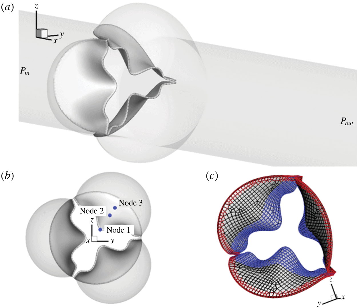
A trileaflet aortic valve model similar to that in Chen & Luo (Reference Chen and Luo2018) is adopted and shown in figure 1. The aorta is simplified as a rigid cylindrical tube with a diameter, $D=2.1~\text{cm}$, and a length, $L=19~\text{cm}$. The three protruded lobes on the tube represent the aortic sinuses and their dimensions are based on physiological measurements of a human aortic root (Swanson & Clark Reference Swanson and Clark1974; Reul et al. Reference Reul, Vahlbruch, Giersiepen, Schmitz-Rode, Hirtz and Effert1990). The geometry of the leaflets was based on a transcatheter aortic valve (known as TAV) (Mao et al. Reference Mao, Li and Sun2016) and was originally provided by Professor Wei Sun’s lab at the Georgia Institute of Technology. The thickness of the human aortic valve, $h$, can range from 0.26 mm to 1.3 mm for normal hearts (Sahasakul et al. Reference Sahasakul, Edwards, Naessens and Tajik1988) but could be thinner for transcatheter valves, e.g. 0.16 mm for a polyurethane valve (Wu et al. Reference Wu, Pott, Mazza, Sironi, Dordoni, Chiastra, Petrini, Pennati, Dubini and Steinseifer2016) and 0.18 mm for a pericardial bioprosthetic valve (Li & Sun Reference Li and Sun2010). The native aortic valve is typically asymmetric and also non-uniform in thickness (Sahasakul et al. Reference Sahasakul, Edwards, Naessens and Tajik1988), but we assume a symmetric model and uniform thickness for simplicity. To vary the leaflet thickness, we extrude the mesh of the leaflets along the surface normal direction in the ANSYS ICEM package to obtain eight different valve models, whose thickness is $h=0.05$, 0.08, 0.1, 0.2, 0.3, 0.5, 0.6 and 0.8 mm, respectively. The small-thickness cases with $h\leqslant 0.1~\text{mm}$ are included as a theoretical exploration of this study. The model with $h=0.1~\text{mm}$ was constructed in our previous study (Chen & Luo Reference Chen and Luo2018), and we will include some of results from that study in the present work for comparison.

Figure 1.

(a) Computational model of the aorta root, where the aorta tube and the aortic valve are affixed together. (b) Axial view of the valve and three sinuses, where the three markers on a leaflet are used later to plot the displacement history. (c) The fixed nodes (red markers) and contact detection region (blue markers).

Figure 2.

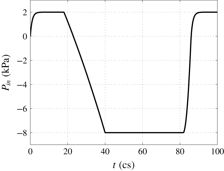
Pressure load applied at the inlet of the aorta tube in the FSI simulation, where cs denotes centiseconds.

For spatial discretization, the rigid aortic wall is divided into 20 735 triangular elements with mesh refinement in the sinus region (approximately 0.3 mm in size). The valve tissue has a separate mesh, where each leaflet is discretized using 539 to 806 20-node hexahedron elements. These elements use quadratic basis functions and have higher-order accuracy than the 4-node tetrahedral elements that use linear basis functions. The valve is then attached to the aorta with fixed element nodes in the commissure region and also along the base, as shown in figure 1(a). A slightly open valve is used as the initial condition. A contact detection region shown in figure 1(c) is prescribed on the left-ventricle side of the surface for each leaflet, within which all the surface nodes will be checked in the simulation to determine whether or not to invoke the contact algorithm. Three nodes in figure 1(b), one located at the centre of the free edge and the other two in the belly region, are traced to show kinematics of the leaflets.

Constitutive models of the valve tissue have been advanced to include fibre orientation and anisotropic effects (Billiar & Sacks Reference Billiar and Sacks2000). However, a simple isotropic neo-Hookean model should be sufficient for simulation of flexural deformation (Fan & Sacks Reference Fan and Sacks2014). Thus, we assume that the leaflet tissue is isotropic and homogeneous, and we adopt the Saint Venant–Kirchhoff model for the hyperelastic tissue behaviour in which the nonlinear strains are incorporated. The density of the leaflets is $\unicode[STIX]{x1D70C}_{s}=1~\text{g}~\text{cm}^{-3}$. The mass damping coefficient, $\unicode[STIX]{x1D702}_{d}$, is chosen so that $\unicode[STIX]{x1D702}_{d}h=1~\text{g}~\text{cm}^{-2}~\text{cs}^{-1}$ is constant for all valve models (cs or centisecond is the time unit in the present study unless otherwise specified). This structural damping is much smaller in comparison with the damping effect provided by the fluid and is added to be consistent with the previous case of $h=0.1~\text{mm}$. For the material properties, we set Young’s modulus to $E=1500~\text{kPa}$ and Poisson’s ratio to $\unicode[STIX]{x1D708}_{s}=0.4$ (Hsu et al. Reference Hsu, Kamensky, Xu, Kiendl, Wang, Wu, Mineroff, Reali, Bazilevs and Sacks2015; Kamensky et al. Reference Kamensky, Hsu, Schillinger, Evans, Aggarwal, Bazilevs, Sacks and Hughes2015).

The blood is assumed to be Newtonian and incompressible. No-slip and no-penetration boundary conditions are imposed at the aorta wall as well as the leaflet surface. The fluid domain is a $19\times 4.4\times 4.4~\text{cm}^{3}$ rectangular bounding box and is discretized by a $400\times 130\times 130$ non-uniform Cartesian grid. Finer resolution with $\unicode[STIX]{x0394}x=0.025~\text{cm}$ and $\unicode[STIX]{x0394}y=\unicode[STIX]{x0394}z=0.034~\text{cm}$ is used in the region surrounding the valve. The flow is driven by a physiological pressure drop along the aorta. The density and dynamic viscosity of the blood are $\unicode[STIX]{x1D70C}=1~\text{g}~\text{cm}^{-3}$ and $\unicode[STIX]{x1D707}=0.005~\text{Pa}~\text{s}$, respectively. Each cardiac cycle has a time duration of $T=0.86~\text{s}$, or 86 cs, which corresponds to a heart rate of 70 beats per minute. Similar to previous aortic valve models (Hsu et al. Reference Hsu, Kamensky, Xu, Kiendl, Wang, Wu, Mineroff, Reali, Bazilevs and Sacks2015; Mao et al. Reference Mao, Li and Sun2016), a transient transvalvular pressure load as shown in figure 2 is applied at the inlet of the aorta tube to drive the flow. The peak pressure during systole is $P_{max}=2~\text{kPa}$, and the lowest pressure during diastole is $-8~\text{kPa}$. The exit pressure at the outlet is $P_{out}=0~\text{kPa}$.

To solve the governing equations, we use a computational framework that was previously developed for simulating biological systems that involve large deformations (Tian et al. Reference Tian, Dai, Luo, Doyle and Rousseau2014). In this partitioned FSI framework, the flow is solved using a Cartesian grid based direct-forcing immersed-boundary method, and the solid is solved using a nonlinear finite-element method on an unstructured Lagrangian mesh (Doyle Reference Doyle2008, Reference Doyle2009). Fluid–structure interaction coupling is achieved by iterating the two solvers while communicating boundary conditions at each time step until convergence. The code was verified through various case studies, including both thin-walled and general 3-D body problems (Tian et al. Reference Tian, Dai, Luo, Doyle and Rousseau2014). More information is provided in § A.1. In the current FSI iteration, the relaxation factors are chosen as $\unicode[STIX]{x1D6FC}=0.7$ for the velocity update, $\unicode[STIX]{x1D6FC}=0.9$ for the force update and $\unicode[STIX]{x1D6FC}=1.0$ for the displacement update. To ensure numerical stability of the FSI coupling, the time step used for the flow solver is $\unicode[STIX]{x0394}t=8.0\times 10^{-3}~\text{cs}$. The time step for the structural simulation is smaller, $\unicode[STIX]{x0394}t=5.0\times 10^{-5}~\text{cs}$, so that each FSI step contains 160 substeps for the structural simulation.

For parallel computing, the rectangular box containing the flow domain is divided into $26\times 26$ subdomains in the $y$- and $z$-directions using domain decomposition. Each subdomain only stores its own flow field data but has a full copy of the unstructured mesh of the fluid–solid interface. Since the surface mesh data for the solid is much smaller as compared with the volume data of the flow field, this decomposition strategy allows nearly a constant scaling of the total computer memory regardless of the number of processor cores being used for the simulation. In the present study, a total number of 692 processor cores (676 for flow and 16 for solid) are used for the FSI simulation, which takes approximately 50 hours for one cardiac cycle on Stampede 2 at the Texas Advanced Computing Center (TACC).

2.2 Contact model

During the closing phase and also sometimes in the opening as well, the three leaflets experience significant contact with one another. Similar to previous studies (Borazjani Reference Borazjani2013; Kamensky et al. Reference Kamensky, Hsu, Schillinger, Evans, Aggarwal, Bazilevs, Sacks and Hughes2015), a penalty method is adopted here to model collision and prevent the leaflets from penetration. At each time step, the node-to-surface distance is calculated to determine whether the contact algorithm is invoked or not. That is, for each of the nodes in the contact region shown in figure 1(c), the distance is computed by projecting it onto the surface of its neighbouring leaflets. The contact force in the direction of the surface normal is then calculated by

(2.1)$$\begin{eqnarray}\displaystyle f_{cnt}=\left\{\begin{array}{@{}ll@{}}0,\quad & \text{if}~d-d_{0}>0,\\ -f_{ext}-k(d-d_{0}),\quad & \text{otherwise},\end{array}\right. & & \displaystyle\end{eqnarray}$$

where $f_{cnt}$ is the nodal contact force, $f_{ext}$ is the external force (i.e. the hydrodynamic force) on the node, $d$ is the distance, $k$ is the contact stiffness and $d_{0}$ is a prescribed threshold distance. Within the threshold distance, the external load $f_{ext}$ is cancelled out and a net force of magnitude $-k(d-d_{0})$ is added to prevent inter-penetration of colliding leaflets. The contact force vanishes outside of the threshold distance. Here we set $k=1~\text{g}~\text{cs}^{-2}$ and $d_{0}=0.08~\text{cm}$ so that when the leaflets are stopped by the contact force, the gap between them is below one cell width on the flow mesh (thus, the flow is cut off completely). We ignore the possible lubrication effect for the thin gap between two leaflets, as the exact nature of the contact mechanism should not significantly affect flow or leaflet deformation during the most of the opening and closing phases.

2.3 Mesh refinement study

A mesh refinement study is performed for the case of thickness $h=0.3~\text{mm}$, where the flow domain is divided by a $500\times 260\times 260$ non-uniform Cartesian grid and the resolution around the leaflets is $\unicode[STIX]{x0394}x=0.015~\text{cm}$ and $\unicode[STIX]{x0394}y=\unicode[STIX]{x0394}z=0.017~\text{cm}$. 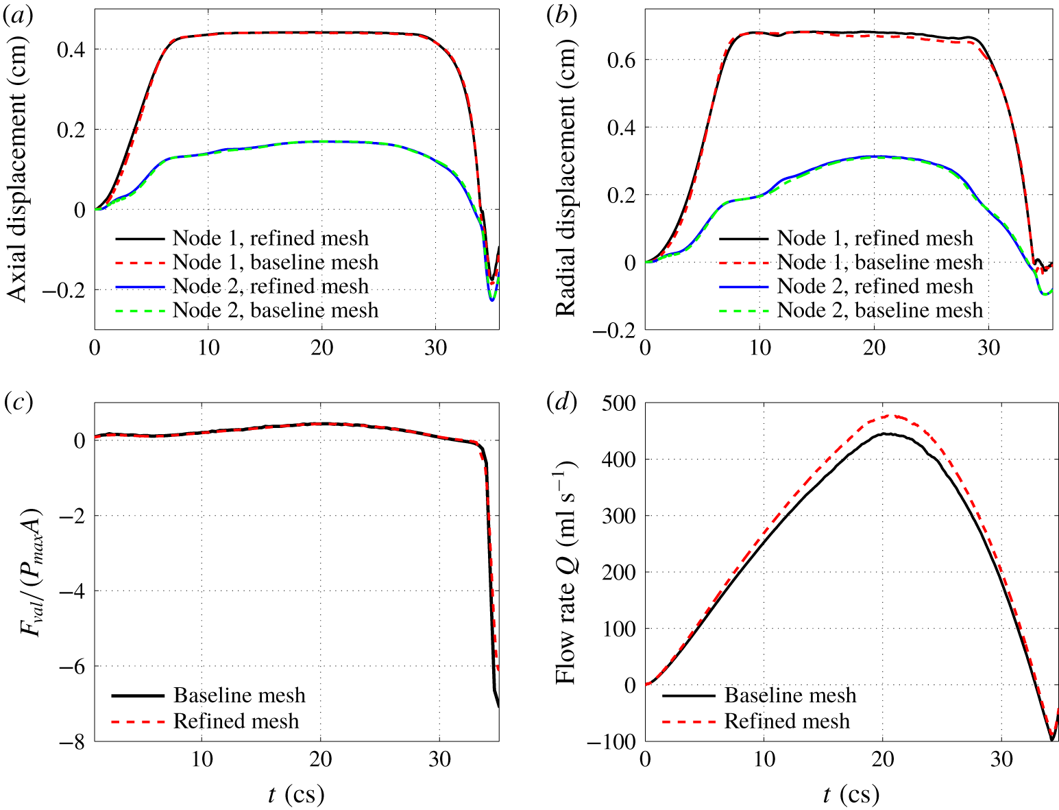The time step size is $\unicode[STIX]{x0394}t=4.0\times 10^{-3}~\text{cs}$ and the refined FSI simulation is run up to $36~\text{cs}$ for the entire systole until the valve already reaches full closure. The results are shown in figure 3 for comparison. Figures 3(a) and 3(b) show the transient axial and radial displacements of the traced markers located on the leaflets (i.e. node 1 and node 2 in figure 1). Figures 3(c) and 3(d) show the total axial force on the three leaflets, $F_{val}$, and the flow rate, respectively. From these results, we see that the valve dynamics and the total force on the valve are accurately captured by the baseline mesh, while the flow rate exhibits a less than 7 % error during the peak rate. We also examined the pressure distribution on the leaflet surface using the refined mesh, and the result is included in § A.2. Based on these comparisons, the baseline flow mesh is deemed satisfactory for the current study. We also did a separate mesh refinement study for the finite-element model of the valve, in which the number of hex-20 elements is increased by approximately five times in the refined mesh. Comparison of the leaflet dynamics shows that the results are in excellent agreement with the baseline valve mesh.

Figure 3.

Comparison between the baseline flow mesh and refined flow mesh for (a) axial and (b) radial displacements of the nodes 1 and 2 on the leaflet, (c) the total force on the valve normalized by the pressure load, and (d) the flow rate during entire systole.

Figure 4.

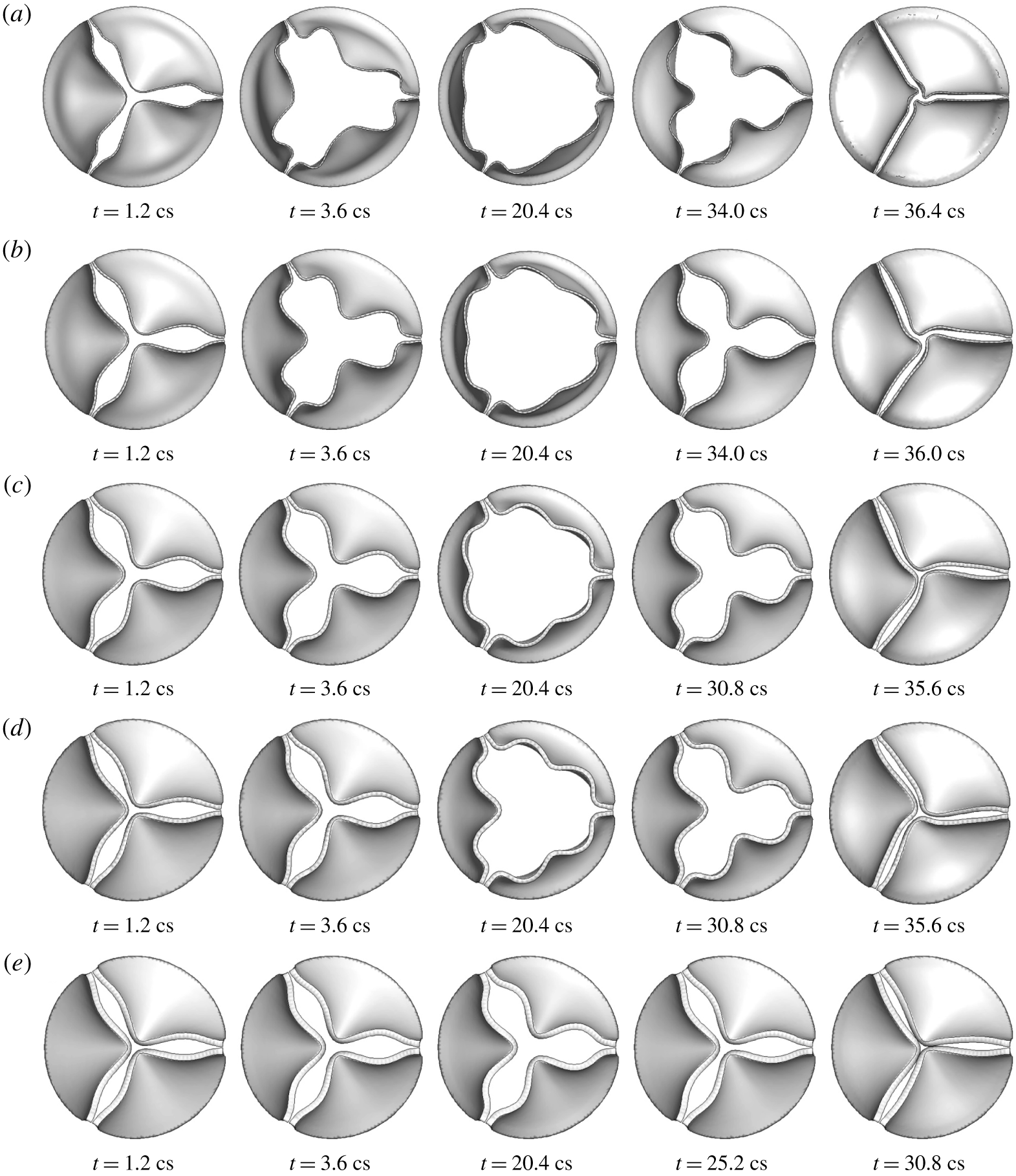
Deformation of the valve in 3-D FSI simulation for thickness (a) $h=0.2~\text{mm}$, (b) 0.3 mm, (c) 0.5 mm, (d) 0.6 mm, (e) 0.8 mm.

3.1 Leaflet deformation

Figure 4 shows the valve deformation sequence for thickness $h=0.2$ to $0.8~\text{mm}$. From these plots, it is evident that the bending rigidity has a significant effect on the dynamic shape of the valve and the extent of valve opening. For the thinner leaflets with $h=0.2$ and 0.3 mm, the valve opens up quickly, first bulging out from its belly and then moves its free edges to their full extent. During the closing phase, the leaflets start to contract inward, again first from the belly area and then the free edges follow up. Because the mid-edge moves ahead of rest of the free edge, each leaflet forms an inward fold at the mid-edge. During diastole, the leaflets are stretched inward with a clear extension by the negative ventricle pressure. For $h=0.1~\text{mm}$, the deformation pattern is similar to that described here, but the leaflets are so flexible in that case that they also form a travelling wave from the base to the free edge, causing the leaflets to flap like immersed flags after the valve is fully opened (Chen & Luo Reference Chen and Luo2018). The two thinnest cases, $h=0.05$ and 0.08 mm, have a similar flapping motion to the case of $h=0.1~\text{mm}$ (see movie 1 for leaflet deformation, available at https://doi.org/10.1017/jfm.2019.904, in these cases). Such a flapping motion was confirmed in our previous study (Chen & Luo Reference Chen and Luo2018) using mesh and time step refinement.

For the intermediate thickness of $h=0.5$ and 0.6 mm, the valve opening is clearly slowed down. The leaflet bellies do not bulge out very much, and the free edges are not fully extended, thus creating a smaller opening area for the flow to go through. During the closing phase, the free edges move in first, and then the belly regions follow. The curvature of the mid-edges is not as high as that of the thinner leaflets. For the thickest case of $h=0.8~\text{mm}$, the valve opening is substantially reduced, and the leaflet displacement is less than halfway through.

For all the cases in figure 4, the free edges of the leaflets form an opening with a three-lobe propeller configuration that is consistent with observations in several previous experimental studies of aortic valves (Nakai et al. Reference Nakai, Takeuchi, Yoshitani, Kaku, Haruki and Otsuji2009; Schoenhagen et al. Reference Schoenhagen, Hausleiter, Achenbach, Desai and Tuzcu2011; Machida et al. Reference Machida, Izumo, Suzuki, Yoneyama, Kamijima, Mizukoshi, Takai, Kobayashi, Harada and Miyake2015) as well as FSI simulations (Van Loon Reference Van Loon2010; Kamensky et al. Reference Kamensky, Hsu, Schillinger, Evans, Aggarwal, Bazilevs, Sacks and Hughes2015; Mao et al. Reference Mao, Li and Sun2016; Chen & Luo Reference Chen and Luo2018; Spühler et al. Reference Spühler, Jansson, Jansson and Hoffman2018). This particular shape is caused by the inward fold at the mid-edge of the leaflets that has a higher stiffness and has to snap through in order to extend out to form an opposite curvature. For the thinner cases of $h=0.2$ and 0.3 mm, snap through is easier and can happen later at the full opening of the valve. For thicker cases of $h=0.5$ and 0.6 mm, snap through becomes more difficult. For $h=0.8~\text{mm}$, snap through becomes impossible with the given ventricle pressure load, and therefore, the propeller configuration is maintained during the whole systole in this case. For $h=0.1~\text{mm}$ and less, the valve opens from the middle due to its low bending rigidity and thus, the valve forms a three-lobe star shape instead during the initial opening phase (see supplementary material 1 for leaflet deformation in these cases).

3.2 Flow rate and valve opening area

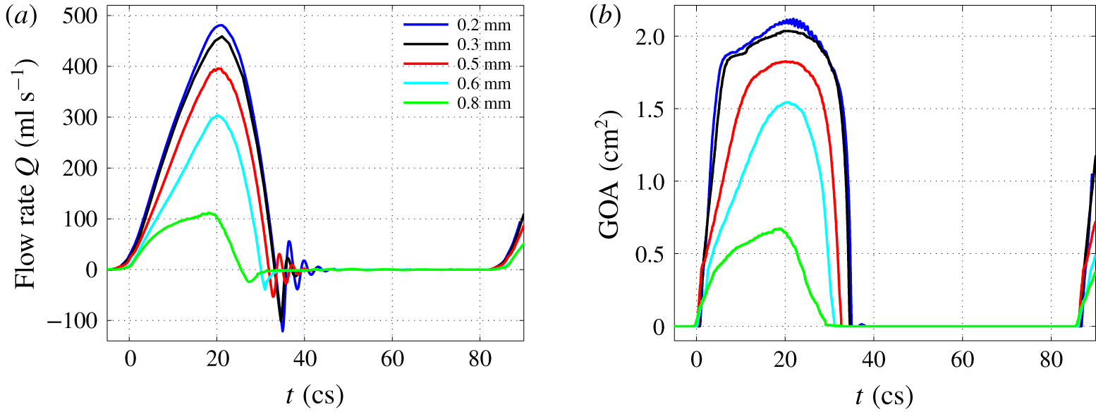
Figure 5(a,b) presents the transient flow rate, $Q=\int u\,\text{d}A$, and geometric orifice area (GOA) from an entire cardiac cycle for all five different cases. The GOA is calculated by finding the projected area of the valve on a plane perpendicular to the aorta axis. The effect of the bending rigidity is evident from this figure. As the thickness increases, the flow rate and the opening area during the systole drop significantly, especially for the cases of $h=0.6$ and 0.8 mm. Note that from the specified pressure waveform in figure 2, the driving ventricle pressure at the inlet starts to drop at $t=18~\text{cs}$. However, the forward flow continues to accelerate under the positive pressure load until around $t=20~\text{cs}$ when both the flow and GOA reach a peak. The peak flow rate is 483, 459, 396, 304 and $112~\text{ml}~\text{s}^{-1}$ for the case of $h=0.2$, $0.3$, $0.5$, $0.6$ and $0.8~\text{mm}$, respectively.

Figure 5.

Volumetric flow rate, $Q$, and geometric orifice area in a full cardiac cycle for $h=0.2$ to 0.8 mm.

During the closing phase, the thinner valves have a faster moving speed as seen from the time derivative of the GOA. However, the thicker valves close earlier from both the flow rate and GOA plots, which is due to the low flow rate and smaller GOA at the opening phase in these cases. A negative dip in the flow rate is observed for all the cases, indicating a temporary flow reversal that takes place along with the closing motion of the leaflets. By integrating the transient flow rate in time, we obtain the stroke volume for each valve model, which is 98.5, 99.6, 75.3, 52.0 and 20.3 ml per beat for a thickness of $h=0.2$, $0.3$, $0.5$, $0.6$ and $0.8~\text{mm}$, respectively. The corresponding cardiac output (or averaged flow rate) is 6.9, 7.0, 5.3, 3.6 and $1.4~\text{l}~\text{min}^{-1}$. The peak flow rate, stroke volume and cardiac out in the cases of$h=0.2$, $0.3$ and $0.5~\text{mm}$ are all within the physiological range for normal adult aortic valves (Leyh et al. Reference Leyh, Schmidtke, Sievers and Yacoub1999; Hall Reference Hall2015), while in the cases of $0.6$ and $0.8~\text{mm}$ these variables are below the normal range due to reduced valve opening.

The effective orifice area (EOA) represents a measurement of the valve’s characteristic resistance and is often used clinically for the quantification of valve stenosis severity (Yoganathan et al. Reference Yoganathan, He and Casey Jones2004; Peck et al. Reference Peck, Wang, Shaw and Dart2016). The EOA in our calculation follows the previous definition (Yoganathan et al. Reference Yoganathan, He and Casey Jones2004), $\text{EOA}~(\text{cm}^{2})=Q_{rms}/$$(51.6\sqrt{\unicode[STIX]{x0394}p})$, where $Q_{rms}$ is the root mean square systolic flow rate in $\text{ml}~\text{s}^{-1}$ and $\unicode[STIX]{x0394}p$ is the mean systolic pressure drop in mmHg. We used the time period when the pressure difference $P_{in}-P_{out}$ is positive to compute the average as $\unicode[STIX]{x0394}p$. According to this formula, the EOA is 1.81, 1.72, 1.46, 1.11 and $0.49~\text{cm}^{2}$ for a thickness of $h=0.2$, $0.3$, $0.5$, $0.6$ and $0.8~\text{mm}$, respectively. For thinner leaflets (e.g. 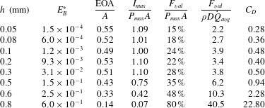$h=0.2$ and 0.3 mm), the EOAs are in agreement with earlier reported results for normal adult valves (Yoganathan et al. Reference Yoganathan, He and Casey Jones2004; Mao et al. Reference Mao, Li and Sun2016). As the thickness increases, the leaflets behave like calcified or stenotic valves and the EOA drops significantly. Regurgitation is the leakage of blood backward through the aortic valve to the left ventricle during diastole. In the current simulation, the regurgitation volume in all the cases is less than 1.3 ml per cycle and is also in good agreement with previous reports (Yoganathan et al. Reference Yoganathan, He and Casey Jones2004; Mao et al. Reference Mao, Li and Sun2016). The performance index of the valve, defined as EOA/$A$ and used in clinical contexts as a criterion to evaluate the severity of valve stenosis, is 0.53 for $h=0.2~\text{mm}$ but drops to only 0.14 for $h=0.8~\text{mm}$. This index is listed later in table 1 along with the normalized valve force for all the cases.

Table 1.

Normalized bending rigidity $E_{B}^{\ast }$, performance index $\text{EOA}/A$, average maximum momentum flux $I_{max}$, average valve force $F_{val}$, and average drag coefficient $C_{D}$ for each case. The case of $h=0.1~\text{mm}$ is from Chen & Luo (Reference Chen and Luo2018).

In general, the valve opening–closing process can be divided into four stages: (i) rapid valve opening, (ii) maintenance of maximum excursion, (iii) slow valve closing, and (iv) fast valve closing (Thubrikar, Heckman & Nolan Reference Thubrikar, Heckman and Nolan1993; Leyh et al. Reference Leyh, Schmidtke, Sievers and Yacoub1999). For the cases of $h=0.2$ and $0.3~\text{mm}$, these four stages can be clearly observed from the GOA plot. In these cases, the rapid valve opening takes approximately 5 to 6 cs, the maximum excursion approximately 19 cs, the slow closing approximately 7 cs, and the fast closing approximately 3 to 4 cs. These time scales agree well with the previously reported data for healthy aortic valves (Yoganathan et al. Reference Yoganathan, He and Casey Jones2004; Mao et al. Reference Mao, Li and Sun2016). As the thickness further increases from $0.5$ to $0.8~\text{mm}$, the maximum excursion stage (represented by a plateau in the transient GOA history) vanishes gradually.

Figure 6.

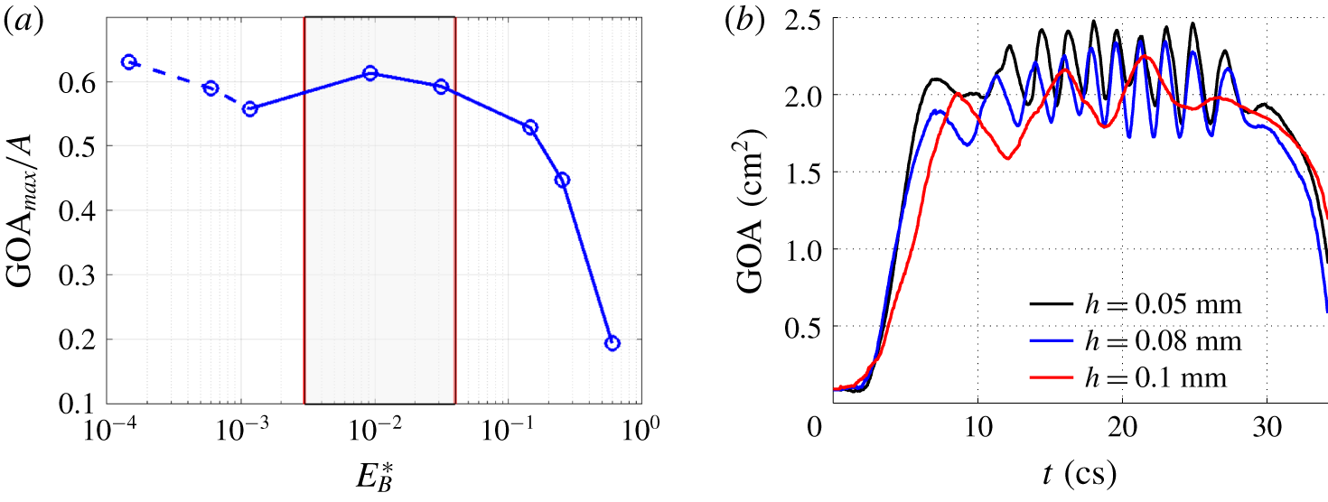
(a) Effect of the normalized bending rigidity on the normalized maximum GOA. The case of $h=0.1~\text{mm}$ from Chen & Luo (Reference Chen and Luo2018) has been included. The dashed part indicates that the leaflets undergo significant flapping oscillations. The shaded area represents approximately the optimal region. (b) Transient GOA for the three thinnest valve cases showing large oscillations.

In the three cases of $h=0.1~\text{mm}$ and less, the time scales of the four stages are similar to those in the cases of $h=0.2$ and 0.3 mm. However, in those cases, the thin leaflets exhibit a flag-like flapping motion after the valve is fully opened (Chen & Luo Reference Chen and Luo2018), which leads to significant oscillations in the GOA (figure 6b). The magnitude and frequency of flapping in those cases are different and may have to do with the bending stiffness, tension in the leaflets, as well as the curvature of the leaflet surface once the valve is opened. For thicker valves, only the case of $h=0.2~\text{mm}$ has such high-frequency oscillations in the GOA and the magnitude is very small as seen in figure 5(b); in the other cases, no evident flapping motion is observed. As a result of the leaflet flapping, the jet in the cases of $h\leqslant 0.1~\text{mm}$ also becomes more oscillatory. For $h=0.05$, 0.08 and 0.1 mm, the flow rate is 504, 479, $447~\text{ml}~\text{s}^{-1}$, respectively, and the EOA is 1.89, 1.79 and $1.67~\text{cm}^{2}$, respectively. Note that the case of 0.1 mm, whose $E_{B}^{\ast }=0.0012$, has reduced flow rate, EOA and GOA when compared with the case of 0.2 mm (figure 6a and table 1). Thus, the changes of valve opening and flow rate are not monotonic as the thickness is reduced from 0.2 mm.

We further present the effect of the bending rigidity on the valve opening in terms of non-dimensional parameters. Figure 6 shows the normalized maximum GOA by the cross-sectional area of the aorta tube, $A$, against the bending rigidity normalized by the overall pressure gradient $\unicode[STIX]{x0394}P/L$, i.e. $E_{B}^{\ast }=E_{B}/(\unicode[STIX]{x0394}PR^{4}/L)$, where $\unicode[STIX]{x0394}P=P_{max}-P_{out}$ is the pressure drop during valve opening, $E_{B}=Eh^{3}/12(1-\unicode[STIX]{x1D708}^{2})$ is the flexural rigidity, $L$ is the tube length and $R$ is the radius of the aorta tube. From figure 6(a), there exists an optimal range of normalized bending rigidity of the valve that is roughly between $E_{B}^{\ast }=0.003$ and 0.04. It is worth noting that most of previous studies of normal aortic valves, including native and prosthetic, fall within this optimal range (Sahasakul et al. Reference Sahasakul, Edwards, Naessens and Tajik1988; Bernacca et al. Reference Bernacca, O’Connor, Williams and Wheatley2002; Mao et al. Reference Mao, Li and Sun2016). Above the range, the valve may become too stiff with the valve opening reduced. In reality the heart would have to do extra work through physiological control mechanisms in the body to maintain sufficient cardiac output; in that case, the normalized bending rigidity $E_{B}^{\ast }$ is effectively reduced due to higher pressure load. On the other hand, below this range the leaflets are too flexible and may form travelling waves and flapping motions, which is typically seen in immersed flags (Shelley & Zhang Reference Shelley and Zhang2011) and could cause the valve performance to drop as in the case of $h=0.1~\text{mm}$. In the design of transcatheter valves, the leaflet thickness is sometimes reduced to accommodate the valve to miniaturized catheters (Abbasi & Azadani Reference Abbasi and Azadani2017). The present finding of the hydrodynamic consequence for very thin leaflets may serve as a design consideration for such valves. Even if sufficient valve opening could still be achieved (as in the cases of $h=0.05$ and 0.08 mm), frequent oscillation of the leaflets due to flapping may become a concern for the cyclic flexural fatigue of bioprosthetic valves (Mirnajafi, Zubiate & Sacks Reference Mirnajafi, Zubiate and Sacks2010).

The definition of the dimensionless parameter $E_{B}^{\ast }$ involves the use of the average pressure gradient along the tube during valve opening, where the tube length has been included in the scaling. To confirm that the results are relatively independent of the tube length and the pressure gradient is a reasonable reference for scaling, we have doubled the tube length, with the tube segments upstream and downstream of the valve both lengthened and the driving pressure at the inlet also doubled. The transient GOA for $h=0.3~\text{mm}$ from this additional FSI simulation is provided as a supplementary figure (see supplementary material 2). The result is consistent with that from the baseline simulation, despite small differences being observed (such differences are expected since the pressure drop should not be strictly proportional to the tube length due to the presence of the valve).

3.3 Pressure distribution

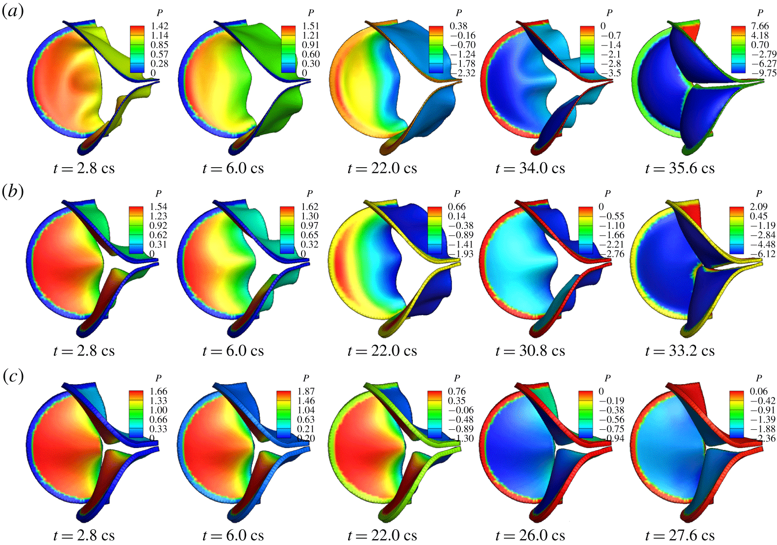
Pressure distribution on the valve surface is a result of two-way interaction between the flow and the leaflets. Thus, not only the instantaneous shape of the valve but also the motion of the leaflets affect the magnitude and spatial characteristics of the surface pressure. Figure 7 shows the pressure on the ventricle side of the valve for $h=0.2$, 0.5 and 0.8 mm at selected systolic moments. It can be seen that at most of these time frames, the surface pressure varies from the base to the free edge of the leaflets. Overall, the pressure drops along the axial direction from the fixed base to the free edge since the valve forms a converging nozzle while opening and the fluid velocity is highest at the exit of the valve. However, the effect of the leaflet movement can be seen as well. For example, comparing the frame of $h=0.2~\text{mm}$ and $t=2.8~\text{cs}$ and the frame of $h=0.5~\text{mm}$ and $t=6.0~\text{cs}$, the amount of valve opening is similar in these two frames, but the pressure is significantly different. In particular, the pressure near the base of the valve in the former frame has a lower magnitude than the pressure at the same region in the latter frame; furthermore, the pressure in the former frame has less variation and is more uniform from the base to the free edge. This result has to do with the fast valve opening in the case of $h=0.2~\text{mm}$, where the thin leaflets yield to the accelerating flow more quickly and thus incur less impact from the flow.

Figure 7.

Pressure distribution (kPa) on the valve in 3-D FSI simulation for thickness (a) $h=0.2~\text{mm}$, (b) 0.5 mm, (c) 0.8 mm. Note that the colour range is different in each frame and colours at the fixed edges are not meaningful.

For the thickest valve of $h=0.8~\text{mm}$, the characteristics of pressure distribution do not change substantially in time during opening due to slow motion of the leaflets, even though the overall magnitude of the pressure still varies temporally according to the pressure waveform specified at the inlet. In all the cases, the pressure on the ventricle side of the valve becomes nearly uniform when the valve is fully closed as seen in the last column in figure 7. In addition, the pressure on the aortic side of the valve is always nearly uniform, though its magnitude depends on the overall shape and movement of the valve.

3.4 Momentum balance and total force on the valve

In order to better understand the total hemodynamic force on the valve, or the valve’s resistance to the flow, we consider the interior of the aortic wall as a control volume and analyse the momentum balance of the flow. The momentum conservation of the flow in the axial direction is

(3.1)$$\begin{eqnarray}\displaystyle \frac{\unicode[STIX]{x2202}}{\unicode[STIX]{x2202}t}\int \unicode[STIX]{x1D70C}u\,\text{d}V+\int \unicode[STIX]{x1D70C}u^{2}\,\text{d}A=(P_{in}-P_{out})A-F_{val}-F_{sin}-F_{tub}, & & \displaystyle\end{eqnarray}$$

where $u$ is the axial velocity, $A=\unicode[STIX]{x03C0}D^{2}/4$ is the area of the cross-section, $P_{in}$ and $P_{out}$ are the inlet and outlet pressure, respectively, $F_{val}$ is the total axial hemodynamic force on the leaflet surfaces (both aortic and ventricle sides included) or the valve resistance, $F_{sin}$ is the axial force on the sinus section of the wall and $F_{tub}$ is the axial force on the remaining tube wall. Introducing the flow rate, equation (3.1) can be written as

(3.2)$$\begin{eqnarray}\displaystyle (P_{in}-P_{out})A=\unicode[STIX]{x1D70C}L\dot{Q}+\int _{\text{out}}\unicode[STIX]{x1D70C}u^{2}\,\text{d}A-\int _{\text{in}}\unicode[STIX]{x1D70C}u^{2}\,\text{d}A+F_{val}+F_{sin}+F_{tub}, & & \displaystyle\end{eqnarray}$$

where $\dot{Q}$ is the time derivative of the flow rate and $L$ is the length of the flow domain. This equation represents how the transvalvular pressure load is split among different factors that include the inertial acceleration of the fluid column in the aorta, momentum fluxes, and the forces on the valve, sinuses, and tube wall. As shown in our previous study (Chen & Luo Reference Chen and Luo2018), the momentum fluxes at the inlet and outlet nearly cancel each other; furthermore, $F_{sin}$ and $F_{tub}$ are small. Thus, the overall pressure load is mostly shared between flow acceleration and the force on the valve, i.e. $(P_{in}-P_{out})A\approx \unicode[STIX]{x1D70C}L\dot{Q}+F_{val}$, at any time moment.

Figure 8.

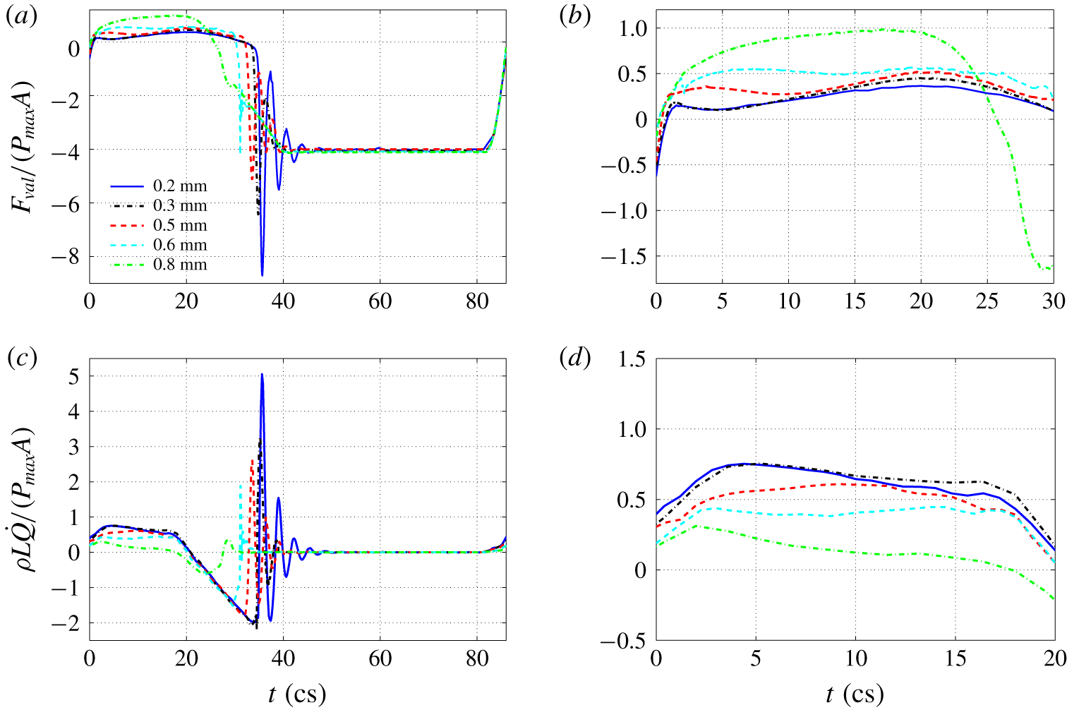
History of normalized (a) $F_{val}$ and (c) $\unicode[STIX]{x1D70C}L\dot{Q}$ for each valve in a full cycle. (b,d) Zoomed-in view of (a,b) for systolic acceleration.

The transient valve force $F_{val}$ and fluid inertial force $\unicode[STIX]{x1D70C}L\dot{Q}$ normalized by $P_{max}A$ are both plotted in figure 8 for an entire cycle. The most distinct feature in the valve force as shown in figure 8(a) is the negative spike that immediately follows full closure of the valve for all the cases except $h=0.8~\text{mm}$. This force is generated when the reversal flow is initiated during the closing phase but is quickly shut off. Due to its momentum, the reversal flow impinges on the aortic side of the valve, leading to a ‘water hammer’ effect and a large resultant force. If the valve is thin and more elastic, the leaflets may be stretched toward the left ventricle by the reversal flow and then bounce back, thus causing several following-up spikes of lower magnitude. An animation of the valve force for $h=0.3~\text{mm}$ is provided as a movie (see supplementary movie 2). As the valve thickness is increased, the magnitude of the force spike becomes lower, and the spike has completely gone for $h=0.8~\text{mm}$. From the inertial force shown in figure 8(b), we see that there are corresponding spikes in $\unicode[STIX]{x1D70C}L\dot{Q}$ that are similar in magnitude but opposite in sign to the valve force.

From the zoom-in plots in figure 8(c,d), it can be seen that for thin leaflets of $h=0.2$ and 0.3 mm, the valve force is much smaller as compared with the fluid inertial force during the acceleration phase of $t=0$ to 20 cs. For the thick leaflets of $h=0.6$ and 0.8 mm, the valve force becomes greater than the fluid inertial force. The effect is further quantified in table 1 using $F_{val}/(P_{max}A)$ and $F_{val}/(\unicode[STIX]{x1D70C}D\dot{Q})$ averaged from the systole. To compute the average, only the time period of positive $F_{val}$ is considered, and the same for $\dot{Q}$. The former represents the percentage of the valve resistance in the total transvalvular pressure load, and the latter represents the equivalent length of the fluid column, in terms of tube diameter, being accelerated. At $h=0.2~\text{mm}$, the valve resistance is 22 % of the transvalvular pressure and is equivalent to accelerating $3.4D$ of fluid column; at $h=0.8~\text{mm}$, the valve resistance reaches 80 % of the transvalvular pressure and is equivalent to accelerating $40.5D$ of fluid column, which would add significant load to the cardiovascular network.

We may use the peak momentum flux at the inlet, $I_{max}=\max \int \unicode[STIX]{x1D70C}u^{2}\,\text{d}A$ to define the drag coefficient of the valve, so that $C_{D}=2F_{val}/I_{max}$. For thinner valves of $h=0.2$ and $0.3~\text{mm}$, $I_{max}$ is 1.52 N. For thicker valves, $I_{max}$ drops quickly and is 1.03, 0.58 and 0.10 N for $h=0.5$, 0.6 and 0.8 mm, respectively. The corresponding drag coefficient is listed in table 1. For $h=0.2~\text{mm}$, $C_{D}$ is 0.40, and for $h=0.8~\text{mm}$, $C_{D}$ reaches a high level of 22.8. In all the resistance measures listed in the table, the case of $h=0.1~\text{mm}$ has higher resistance than the case of $h=0.2~\text{mm}$ due to its flapping motion in the leaflets. The two thinnest cases, $h=0.05$ and 0.08 mm, have lower drag resistance measures as compared to other cases such as $h=0.1$ and 0.2 mm because these extremely thin leaflets have low stretching stiffness in addition to low bending stiffness, thus having a larger opening area.

3.5 Flow field

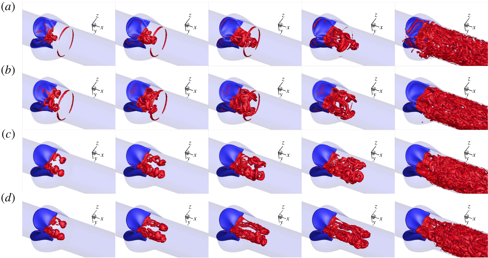
Figure 9 shows a sequence of the vortex structures, plotted using the $Q$-criteria, for selected cases with thickness $h=0.2$, 0.5 and $0.8~\text{mm}$. For comparison, we also included the case of $h=0.1~\text{mm}$ from our earlier work (Chen & Luo Reference Chen and Luo2018). It can be seen that the bending rigidity of the valve has a significant effect on the vortex development. For the case of $h=0.1~\text{mm}$, the flow field is featured by a leading vortex ring first emitting from the central hole of the leaflets and also the second and the third vortex rings that follow the first ring. The first ring is more circular. The second vortex ring initially has a similar 3-lobe star shape to the shape of the initial valve exit, then the ring evolves to a triangular shape before final breakdown (see figure 17 in Chen & Luo (Reference Chen and Luo2018) for more detail). The cases of $h=0.05$ and 0.08 mm have similar vortex patterns.

Figure 9.

Vortex development during valve opening for (a) $h=0.1$, (b) 0.2, (c) 0.5, (d) 0.8 mm at $t=2.8$, $3.6$, $4.4$, $5.2$, $16.4~\text{cs}$.

For all the other five thicker cases considered here, the jet initially forms three separate vortex rings, which originate from the three gaps between any two adjacent leaflets. This behaviour is associated with the propeller shape of valve opening and is caused by the slow opening at the mid-edge of the leaflets where the leaflets fold inward and the effective stiffness is much higher than the rest of the area. In the case of $h=0.2~\text{mm}$, the three vortex rings are interconnected through vortex filaments shedding from the free edge. As the valve continues to open, the axial velocity increases in the central core region, causing the vortex rings to deform. The vortex filaments earlier connecting the three vortex rings penetrate the rings, causing more vortex–vortex interactions, and they travel downstream along with the rings ($t=3.6$ and 4.4 cs) until later breakdown after $t=6~\text{cs}$.

In the cases of $h=0.5$ and 0.8 mm, the three leading vortex rings are more rounded in shape and have less deformation in the first 4 cs. Also, these vortex rings are more independent of each other without evident interconnecting vortex filaments. As the thickness increases, the jet is more confined near the central core region and has a higher velocity due to a limited opening area. For instance, the axial velocity at $t=2~\text{cs}$ is $0.98~\text{m}~\text{s}^{-1}$ for $h=0.3~\text{mm}$, while it is $1.47~\text{m}~\text{s}^{-1}$ for $h=0.6~\text{mm}$ at the same moment, in which case the vortex rings are advected downstream more quickly. In all cases, the vortices become less identifiable later after 16 cs as the flow rate continues to rise. An animation of the vortex structures for $h=0.3~\text{mm}$ is provided as a movie (see supplementary movie 3).

4.1 Model description

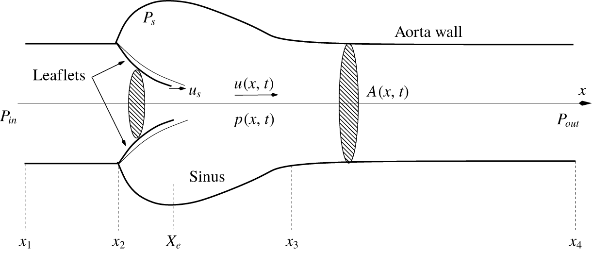
Having better understood the pressure distribution on the valve surface, we proceed to develop a 1-D transient flow model to represent the hemodynamics through the aortic valve. We will combine this flow model with the 3-D finite-element model of the valve to repeat the FSI simulation. Such a hybrid 1-D/3-D FSI model could be useful when high-fidelity representation of the tissue mechanics is needed, e.g. for surgical planning, but simplification of the flow is desired for efficient simulations. To construct the 1-D flow model, we make a few drastic simplifying assumptions to the flow and its geometrical domain. First, we assume that the flow is described only by the axial velocity component, $u(x,t)$, and the pressure has the form of $p(x,t)$. Second, the entire domain is axisymmetric, including the aorta tube and the sinus region, and the trileaflet valve is treated as a nozzle with circular cross-sections but a flexible wall. The schematic of the domain is shown in figure 10 for illustration. The cross-sectional area of the domain at any location is denoted by $A(x,t)$ and is calculated from the actual 3-D geometry of the domain shown in figure 1. At a cross-section that intersects the three leaflets, $A$ is computed by finding the area within an $x$-plane enclosed by the ventricle side of the leaflet surface. Since the free edges of the actual leaflets are not located in the same cross-section before the valve is fully open, an $x$-plane may cut through the free edges and thus the enclosed area is not well defined. In that case, the shape of the free edges upstream the $x$-plane is projected onto the plane, and the total area $A$ is the combination of this projected area and the area formed by the intersection between the $x$-plane and the rest of the valve. This treatment allows the effective cross-section of the jet to be taken into account and $A$ to be continuous from the base to the exit of the valve in the 1-D model. The valve exit is denoted by a Lagrangian point, $X_{e}$, in figure 10. The mass conservation equation of the flow can be written as

(4.1)$$\begin{eqnarray}\displaystyle \frac{\unicode[STIX]{x2202}A}{\unicode[STIX]{x2202}t}+\frac{\unicode[STIX]{x2202}Au}{\unicode[STIX]{x2202}x}-u_{s}\frac{\unicode[STIX]{x2202}A}{\unicode[STIX]{x2202}x}=0, & & \displaystyle\end{eqnarray}$$

where $u_{s}(x)$ is the axial velocity of the leaflets. This equation takes into account the fact that the leaflets are moving in the radial direction as well as in the axial direction, both types of displacement having an effect on the local mass conservation. We calculate the axial velocity $u_{s}$ at each $x$-location by comparing and computing the shift of $A$ in the axial direction from two consecutive time steps.

Figure 10.

Schematic of the axisymmetric domain for the 1-D flow model.

Following the 1-D flow model developed by Cancelli & Pedley (Reference Cancelli and Pedley1985) for a collapsible tube with variable cross-sectional area and later modified by Anderson, Fels & Green (Reference Anderson, Fels and Green2013) to simulate the airflow in the human upper airway, we simplify the $x$-momentum equation of the flow in the entire domain to the following form:

(4.2)$$\begin{eqnarray}\displaystyle & \displaystyle \unicode[STIX]{x1D70C}\frac{\unicode[STIX]{x2202}u}{\unicode[STIX]{x2202}t}+\unicode[STIX]{x1D70C}u\frac{\unicode[STIX]{x2202}u}{\unicode[STIX]{x2202}x}=-\frac{\unicode[STIX]{x2202}p}{\unicode[STIX]{x2202}x}+\unicode[STIX]{x1D70F}\frac{s}{A}, & \displaystyle\end{eqnarray}$$

(4.3)$$\begin{eqnarray}\displaystyle & \displaystyle \unicode[STIX]{x1D70F}=\unicode[STIX]{x1D70F}_{fric}+\unicode[STIX]{x1D70F}_{\unicode[STIX]{x1D712}}, & \displaystyle\end{eqnarray}$$

where $\unicode[STIX]{x1D70F}$ is shear stress including the frictional loss, $\unicode[STIX]{x1D70F}_{fric}$, and additional pressure loss in a diverging channel, $\unicode[STIX]{x1D70F}_{\unicode[STIX]{x1D712}}$, and $s$ is the perimeter of the cross-section. The friction loss, $\unicode[STIX]{x1D70F}_{fric}$, is estimated based on the fully developed laminar flow in a tube with constant cross-section, i.e. $\unicode[STIX]{x1D70F}_{fric}=-2\unicode[STIX]{x1D707}(s/A)\,u$; and $\unicode[STIX]{x1D70F}_{\unicode[STIX]{x1D712}}$ is usually associated with loss of kinetic energy due to flow separation and is calculated according to

(4.4)$$\begin{eqnarray}\displaystyle \unicode[STIX]{x1D70F}_{\unicode[STIX]{x1D712}}=\frac{A}{s}(1-\unicode[STIX]{x1D712})\,\unicode[STIX]{x1D70C}u\frac{\unicode[STIX]{x2202}u}{\unicode[STIX]{x2202}x}, & & \displaystyle\end{eqnarray}$$

where $0\leqslant \unicode[STIX]{x1D712}\leqslant 1$ is a constant representing the amount of pressure recovery in the diverging channel. If $\unicode[STIX]{x1D712}=1$, then $\unicode[STIX]{x1D70F}_{\unicode[STIX]{x1D712}}=0$ and the pressure can be fully recovered (except for the loss due to $\unicode[STIX]{x1D70F}_{fric}$, which is small for the short domain in the present study); and if $\unicode[STIX]{x1D712}=0$, then no pressure is recovered. In the present study, we tested this constant empirically through several simulations. It was found that the following choices work well: in the opening phase, $\unicode[STIX]{x1D712}=0.6$ is set in the region between the valve exit $X_{e}$ and the sinus-tubular junction downstream (i.e. the interval $[X_{e},x_{3}]$ in figure 10), while $\unicode[STIX]{x1D712}=1.0$ elsewhere; after the flow is reversed during the closing phase, $\unicode[STIX]{x1D712}=0$ in the region of $[x_{2},X_{e}]$, $\unicode[STIX]{x1D712}=0.8$ in $[X_{e},x_{3}]$ and $\unicode[STIX]{x1D712}=1.0$ elsewhere.

In the FSI simulation, the fluid pressure from the 1-D flow model is applied axisymmetrically on the left-ventricle side of the 3-D valve so that the surface pressure on this side only depends on $x$ and $t$. On the aortic side, the surface pressure is nearly uniform and is close to the pressure near the valve exit, as we learned from the 3-D FSI simulation. Thus, we assume a uniform sinus pressure, $P_{s}$, on the aortic side of the valve and assume that it is related to the pressure at $X_{e}$, $P_{e}$, by the inertial displacement of the fluid in the entire sinus region,

(4.5)

where  is the instantaneous volume of the sinus region calculated from the actual domain,  is the second-order time derivative of , $R$ is the tube radius, and $c$ is an arbitrary constant and is set equal to $c=0.2$ through several trials.

The 1-D flow is driven by the pressure at the inlet, $p=P_{in}$ at $x_{1}$, which is time dependent and is the same as in the 3-D FSI model. At the outlet $x_{4}$, $p=P_{out}=0$. Equations (4.1) and (4.2) form a boundary value problem that can be solved straightforwardly using a shooting method. Specifically, at a time step where the inlet pressure $P_{in}$ is specified and $A$ is first calculated from the current valve configuration, we assume an inlet velocity $u(x_{1})$ and solve (4.1) using a finite-difference method for $u(x)$ within the entire domain. From this temporary solution of $u(x)$, we then solve (4.2) for temporary pressure $p(x)$, again using a finite-difference method. The pressure solution at the outlet, $p(x_{4})$, is compared with the outlet pressure condition $p=P_{out}$ for a convergence check of this time step. The Newton–Raphson method is adopted for the iterative solution process at each time step. That is, after temporary solutions of $u(x)$ and $p(x)$ are obtained, $u(x_{1})$ is perturbed and the solution process for (4.1) and (4.2) is repeated for a different output of $p(x_{4})$. Then, the numerical derivative $\text{d}p(x_{4})/\text{d}u(x_{1})$ is calculated and used in the Newton iteration until $p(x_{4})$ matches $P_{out}$. Finally, a similar FSI iteration procedure as in the full 3-D simulation is employed here for the hybrid FSI model.

Figure 11.

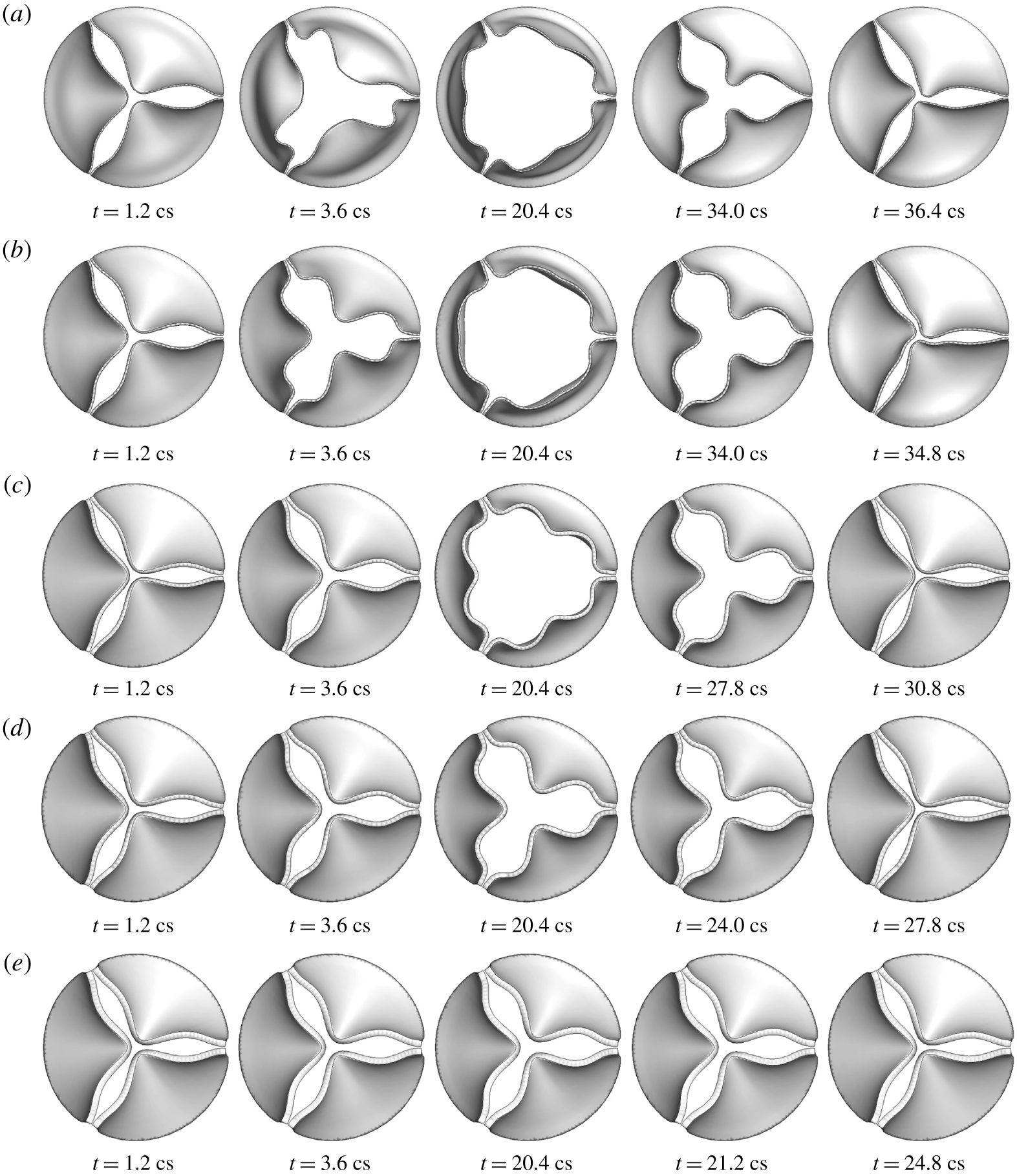
Sequence of valve deformation from hybrid 1-D/3-D FSI simulation for thickness (a) $h=0.2~\text{mm}$, (b) 0.3 mm, (c) 0.5 mm, (d) 0.6 mm, (e) 0.8 mm.

4.2 Results from the hybrid FSI simulation

Figure 11 shows the deformation sequence of the aortic valve at $h=0.2$ to 0.8 mm from FSI simulation using the 1-D flow model. In general, the characteristic deformation pattern agrees well with that from the 3-D FSI simulation. This result is in contrast with the solid-only simulation with a uniform pressure assumption, which leads to overly large displacement and outward bending of the leaflets (Hsu et al. Reference Hsu, Kamensky, Xu, Kiendl, Wang, Wu, Mineroff, Reali, Bazilevs and Sacks2015; Gilmanov & Sotiropoulos Reference Gilmanov and Sotiropoulos2016; Chen & Luo Reference Chen and Luo2018). For thinner leaflets of $h=0.2$ and 0.3 mm, the 1-D flow model produces a correct deformation sequence where the belly of the valve bulges out first and is followed by the free edge opening, and in the other cases, the free edges move ahead of the rest of the valve. Furthermore, the 3-lobe propeller shape of the free edges is preserved for all cases during both the opening and closing phases. 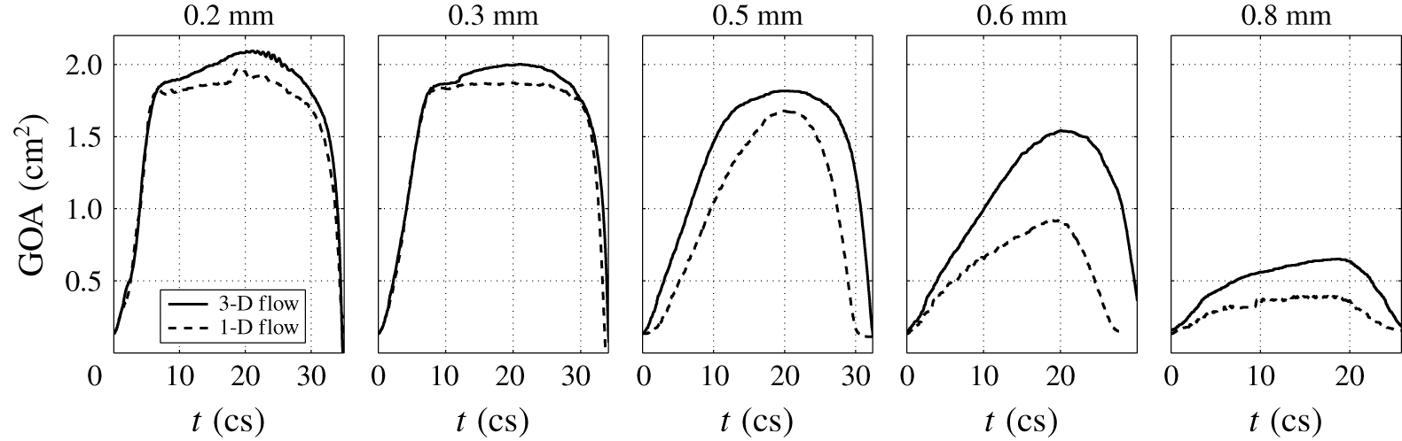The major discrepancy with the 3-D result is that for thicker leaflets of $h=0.6$ and 0.8 mm, the opening of the valve is smaller than the opening from the 3-D FSI result. A detailed comparison is further shown in figure 12 for history of the GOA during the entire systole. For thinner leaflets of $h=0.2$ and 0.3 mm, the 1-D flow model also produces fairly accurate dynamics of the leaflets, i.e. fast opening, maximum excursion, slow closing, and then fast closing of the valve, even though the maximum valve opening in the hybrid simulation is slightly smaller than that in the 3-D simulation. For thicker leaflets of $h=0.6$ and 0.8 mm, there is significant discrepancy between the two models, and the hybrid simulation produces slower opening and closing than the 3-D simulation; however, the overall characteristics are still in qualitative agreement.

The hybrid FSI simulation is stopped once the valve becomes fully closed. Thus, the diastole phase is not included in the simulation. In practice, the 1-D flow model can simply be replaced by a lumped-parameter piston-like model to continue the simulation after valve closure and to capture the subsequent ‘water hammer’ effect.

Figure 12.

Comparison of the GOA history between the 1-D flow and 3-D flow in the FSI simulation.

Figure 13.

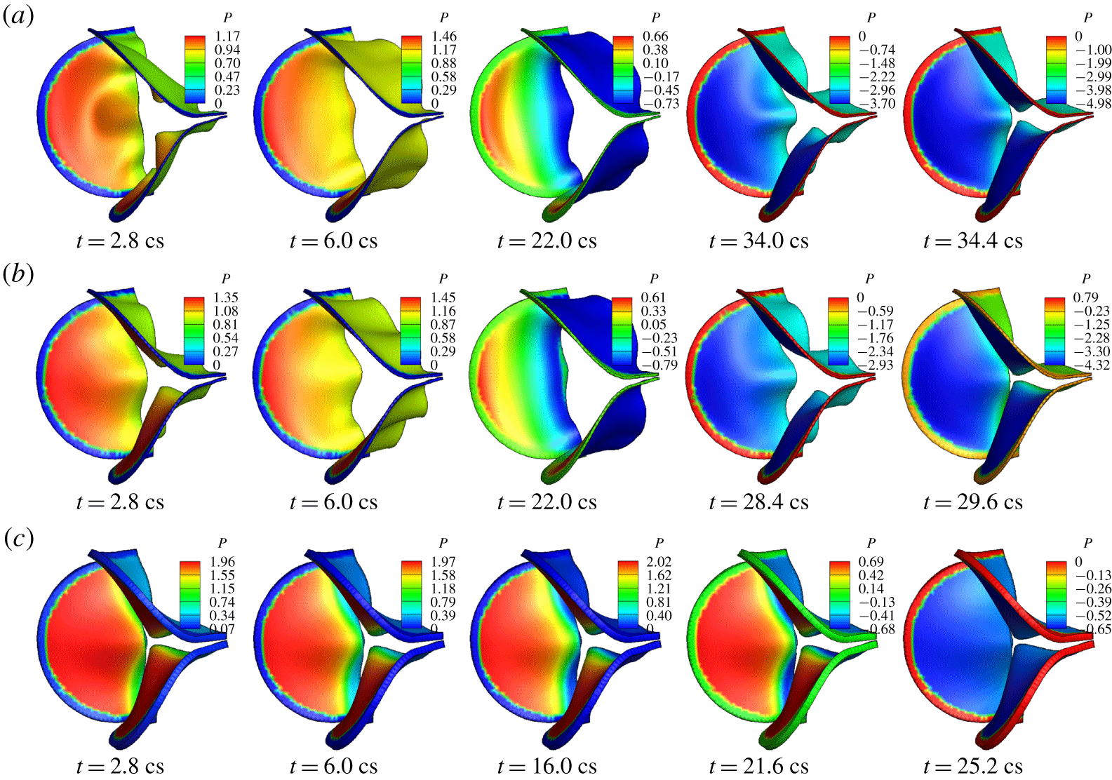
Pressure distribution (kPa) on the valve in hybrid FSI simulation for thickness (a) $h=0.2~\text{mm}$, (b) 0.5 mm, (c) 0.8 mm.

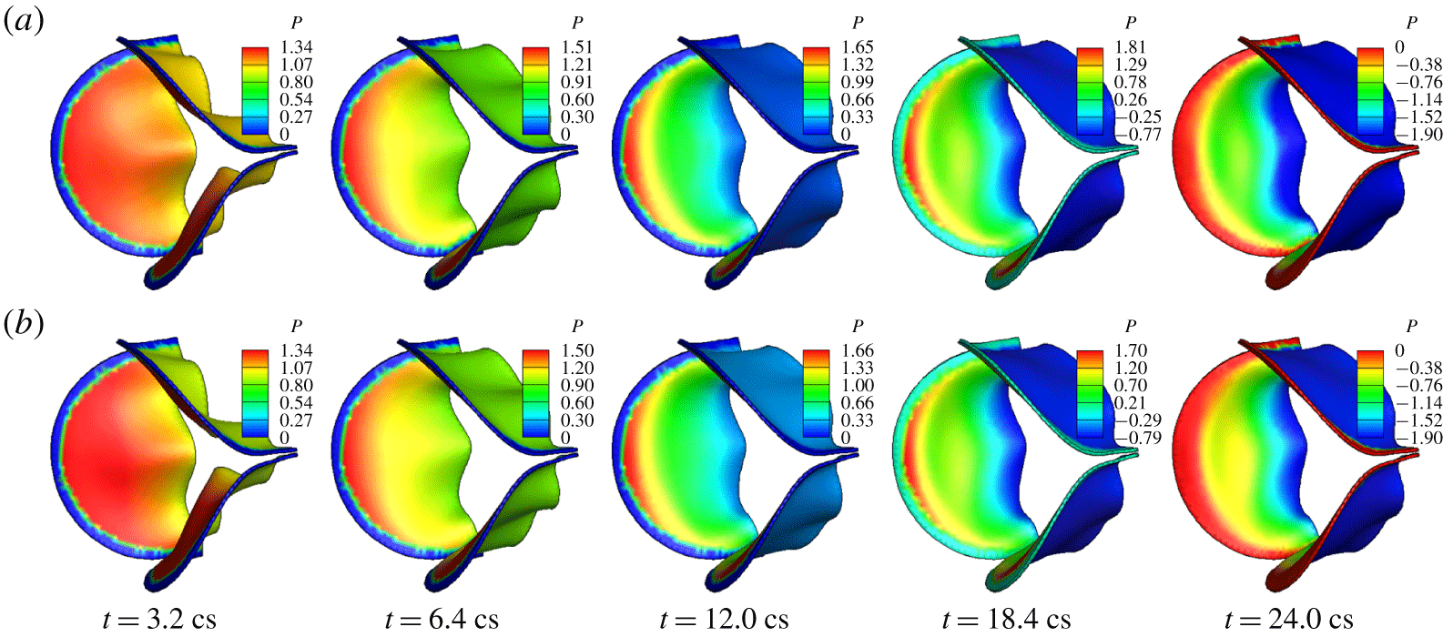
Pressure distribution on the valve surface from the hybrid FSI simulation is shown in figure 13 for all five cases. Comparing the pressure contours with those in the corresponding 3-D simulation as shown in figure 7, we see that the overall non-uniform characteristics are captured by the 1-D flow model: the pressure on the ventricle side drops from the base to the free edge during opening phase, and during closure the pressure on the ventricle side becomes more uniform in the cases $h=0.2$ to 0.6 mm. Furthermore, the pressure on the aortic side varies in time in response to the valve opening in a correct fashion as in the 3-D simulation. Even though the specific magnitude of the pressure may be somewhat different from that in the 3-D simulation, in general the pressure difference between two sides of the valve is still reasonably close to that in the 3-D simulation. Further inspection shows that in the cases of $h=0.6$ and 0.8 mm, the pressure on the ventricle side near the midpoint of the free edges is lower than that in the 3-D simulation. This discrepancy has led to reduced opening of the valve by the 1-D flow in these two cases.

Figure 14.

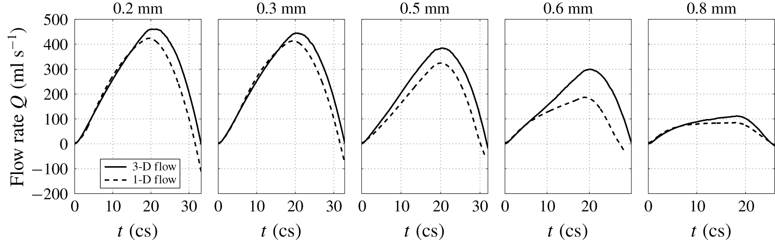
Comparison of the flow rate between the 1-D flow and 3-D flow in the FSI simulation.

Figure 14 shows the history of the flow rate from the hybrid FSI simulation. Again, the major characteristics of the flow are captured reasonably well. For thinner valves of $h=0.2$ and 0.3 mm, the flow rate matches the 3-D result quite well, including rise and drop of the flow rate in the systole and even the temporary negative flow rate right before the full closure. For thicker valves $h=0.5$ and 0.6 mm, there is significant discrepancy between the two models, and the 1-D flow model produces a lower flow rate that is associated with reduced valve opening in the simulation.

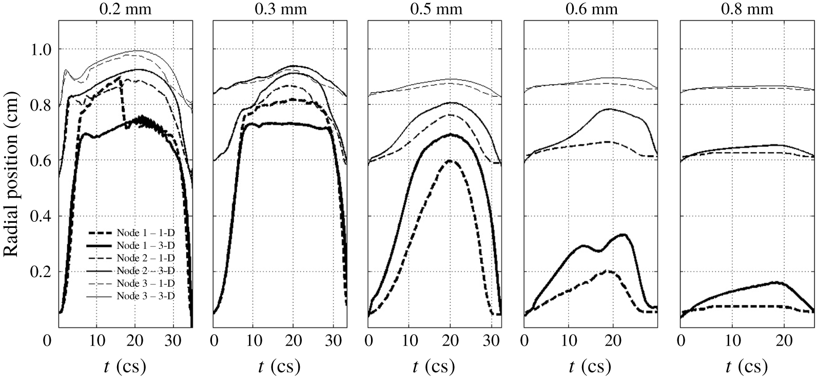
Figure 15 shows a comparison of the leaflet kinematics between the hybrid and full 3-D FSI simulations. In the figure, the radial position of the three selected points on the valve is traced out during systole. These points are marked in figure 1: node 1 on the free edge, node 2 at the belly and node 3 near the base. It can be seen that the hybrid FSI results generally agree with the full 3-D FSI results, indicating that the transient deformation is, overall, consistent between the two simulations. However, there are also notable differences. For example, in the case of $h=0.2~\text{mm}$, the free edge of leaflets first bends more outward in the hybrid FSI simulation before returning to the same position as in 3-D FSI. Since the leaflets are very flexible in this thin case, the valve deformation is more sensitive to the errors in the pressure prediction. In the cases of $h=0.6$ and 0.8 mm, the hybrid simulation clearly under-predicts the valve deformation, and this result has to do with the simplified interpolation of 1-D pressure onto the leaflet surface as discussed earlier.

Figure 15.

Comparison of the radial position for the three marked points on the valve between the 1-D and 3-D flow models in the FSI simulation.

In summary, the present 1-D flow model produces reasonable results when combined with the 3-D tissue model, and it requires drastically less computation as compared with the 3-D flow model. In some of the cases, e.g. valves with high bending rigidity, this 1-D flow model could be further improved by considering interpolating the fluid pressure onto the leaflet surface in an empirical fashion that better matches the pressure contours from the 3-D simulation. Finally, there are several limitations in the present study. We have ignored the anisotropic effects of the tissue and greatly simplified the geometry of the aortic root as well as the inlet/outlet flow conditions. Our models are also limited to a symmetric configuration of the valve, and its possible application to asymmetric and abnormal valves (e.g. bicuspid valves) will need further investigation.