1 Introduction
The year 2016 marks the half-century anniversary of two seminal papers that have revolutionised the study of solitons in plasmas. Remarkably, the two papers applied two different approaches. On the one hand, Washimi & Taniuti (Reference Washimi and Taniuti1966) used reductive perturbation analysis, a subtle method that introduces a small disturbance into a stretched coordinate system. Their results show that such small-amplitude solitons are governed by the Korteweg–de Vries (KdV) equation. The integrability of the KdV equation implies that these solitons have elastic collision properties (Zabusky & Kruskal Reference Zabusky and Kruskal1965; Gardner et al. Reference Gardner, Green, Kruskal and Miura1967). On the other hand, Sagdeev (Reference Sagdeev and Leontovich1966) introduced the more direct pseudopotential method that seeks steady-state solutions in a moving frame. Unlike its counterpart, Sagdeev’s pseudopotential method tells us nothing about the collision properties of these solitons. However, its main advantage is that it retains the full nonlinearity, so that no a priori restrictions are placed on the size of the soliton’s amplitude. Therefore it applies to solitons of small and large amplitudes.
An important characteristic of an electrostatic soliton is its polarity. Solitons can have either positive or negative polarity. For each species, the polarity determines whether the soliton causes a compression or rarefaction. Early studies (Sagdeev Reference Sagdeev and Leontovich1966; Washimi & Taniuti Reference Washimi and Taniuti1966) show that a simple plasma consisting of cold ions and Boltzmann electrons supports only positive polarity solitons. It therefore came as a surprise that certain compositions of a plasma consisting of cold ions and two Boltzmann electron species can support negative polarity ion-acoustic solitons. The soliton properties of this model was first studied by Goswami & Buti (Reference Goswami and Buti1976) via reductive perturbation theory. An unfortunate factorization error led them to the false conclusion that no negative polarity solitons can form, and that large regions in parameter space support no soliton solutions. This conclusion was corrected by Buti (Reference Buti1980) through the use of Sagdeev’s pseudopotential analysis.
More interestingly, coexistence was shown to occur. Coexistence means that the same plasma composition supports two families of soliton solutions, one having positive polarity and the other having negative polarity. This was first reported by Buti (Reference Buti1980), who revisited the model consisting of cold ions and two Boltzmann electron species. She applied Sagdeev’s pseudopotential analysis to show the coexistence of positive and negative polarity solitons. These results were confirmed by Nishihara & Tajiri (Reference Nishihara and Tajiri1981), who studied the same model using reductive perturbation analysis. They found that, at critical compositions, the lowest order of nonlinearity vanishes, so that the usual KdV equation fails. Instead, they introduced a different coordinate stretching that allowed them to derive the modified Korteweg–de Vries (mKdV) equation. They used the mKdV equation to show that it supports solitons of either polarity. Therefore, from a theoretical perspective, the possibility of coexistence was derived through reductive perturbation analysis and Sagdeev analysis.
Since these early findings, the coexistence on ion-acoustic time scales has been reported in many different plasma compositions. Nakamura and Tsukabayashi found experimental evidence of coexistence, in good agreement with theoretical results obtained from reductive perturbation analysis (Nakamura & Tsukabayashi Reference Nakamura and Tsukabayashi1984, Reference Nakamura and Tsukabayashi1985). Verheest (Reference Verheest1988) considered the fast ion-acoustic mode in a plasma consisting of an arbitrary number of ion species (including negatively charged ions) and two Boltzmann electron species. He showed that any such plasma has a critical composition where coexistence arises. Furthermore, coexistence was shown to arise under non-thermal electron distributions (Cairns et al. Reference Cairns, Mamun, Bingham, Boström, Dendy, Nairn and Shukla1995; Baluku & Hellberg Reference Baluku and Hellberg2012; Tribeche, Amour & Shukla Reference Tribeche, Amour and Shukla2012), as well as on dust-acoustic (Mamun, Cairns & Shukla Reference Mamun, Cairns and Shukla1996; Gill & Kaur Reference Gill and Kaur2000; Mendoza-Briceño, Russel & Mamun Reference Mendoza-Briceño, Russel and Mamun2000; Maharaj et al. Reference Maharaj, Pillay, Bharuthram, Reddy, Singh and Lakhina2006) and electron-acoustic (Kakad et al. Reference Kakad, Singh, Reddy, Lakhina, Tagare and Verheest2007; Mbuli et al. Reference Mbuli, Maharaj, Bharuthram, Singh and Lakhina2016) time scales.
More recently, Baluku, Hellberg & Verheest (Reference Baluku, Hellberg and Verheest2010) revisited the model of Goswami & Buti (Reference Goswami and Buti1976). They found that one of the coexisting branches may support an acoustic speed soliton. They used the term ‘nonKdV-like’ to describe such a branch, due to the fact that the amplitude of this family of soliton solutions does not vanish in the acoustic speed limit. Therefore, coexistence usually consists of a KdV-like and a nonKdV-like family of solutions. Since then, acoustic speed solitons were reported in many plasma models (Verheest, Hellberg & Baluku Reference Verheest, Hellberg and Baluku2012; Olivier, Maharaj & Bharuthram Reference Olivier, Maharaj and Bharuthram2015; Mbuli et al. Reference Mbuli, Maharaj, Bharuthram, Singh and Lakhina2016). In addition, acoustic speed double layers and supersolitons were reported by Verheest & Hellberg (Reference Verheest and Hellberg2015a ) for a model consisting of cold positive and negative ions and Cairns-distributed electrons (Verheest, Hellberg & Kourakis Reference Verheest, Hellberg and Kourakis2013).
In a different development altogether, Torvén (Reference Torvén1981) used reductive perturbation analysis to predict the existence of double layer solutions in plasmas. To do this, he studied soliton solutions near a critical plasma composition. He derived the Gardner equation to show that weak double layer solutions can arise. The report by Temerin et al. (Reference Temerin, Cerny, Lotko and Mozer1982) about satellite observations of weak double layers in the auroral region stimulated much interest in the study of such double layers. Bharuthram & Shukla (Reference Bharuthram and Shukla1986) used both reductive perturbation analysis and Sagdeev analysis to study the formation of double layers in a plasma consisting of cold ions and two Boltzmann electron species. They found that the model supported both small- and large-amplitude double layers. A comparison showed that reductive perturbation analysis provides a poor approximation in regions of parameter space where large-amplitude double layers arise. Baboolal, Bharuthram & Hellberg (Reference Baboolal, Bharuthram and Hellberg1990) later showed that the velocity of double layers often arise as a theoretical upper limit to soliton propagation speeds. Double layers were also reported on electron-acoustic (Goswami & Bujarabarua Reference Goswami and Bujarabarua1987) and dust-acoustic (Tagare Reference Tagare1997) time scales.
It is therefore clear from the literature that both the phenomena of coexistence and double layers arise in a wide range of plasma compositions, and on a wide range of time scales. In addition, reductive perturbation studies suggest a relationship between both of these phenomena and critical plasma compositions. It is also clear that there are many studies where reductive perturbation analysis is applied to a particular model. In most of these studies, the analysis and conclusions only apply to the particular model under consideration. Few studies compare the soliton behaviour of different fluid models, despite the many similarities.
We therefore introduce a different approach that allows us to look more generally at small-amplitude solitons in fluid models. Our approach is to apply a two-dimensional Taylor series expansion of the Sagdeev pseudopotential. The series is expanded about the equilibrium electrostatic potential
 $(\unicode[STIX]{x1D719}=0)$
and an acoustic speed
 $M_{0}$
. The advantage of this approach is that it allows us to consider electrostatic solitons in a generalized fluid model at critical and near-critical plasma compositions. No assumptions about time scales or plasma composition are necessary in this description.
In agreement with the literature, we show that there are two different types of behaviour near critical plasma compositions: either coexistence or weak double layers. We show that the sign of the coefficient of the fourth-order term of such a Taylor series expansion determines whether coexistence or weak double layers are formed near the critical composition.
A notable exception to the behaviour described above is when the coefficient of the fourth order also vanishes to form a supercritical plasma composition (Verheest Reference Verheest2015). At such compositions, our analysis breaks down, and higher-order nonlinear terms need to be taken into account. This analysis falls outside the scope of this paper.
Our investigation leads to the discovery of an explicit solution of a small-amplitude acoustic speed soliton for near-critical plasma compositions. We provide the necessary conditions for such solitons to occur, and show that they are Lorentzian pulses with much fatter tails than regular solitons. We also perform a case study on a fluid model for a plasma consisting of cold ions and two-temperature Boltzmann electrons. For this model, we derive the same Lorentzian acoustic speed soliton from reductive perturbation theory. In particular, we show that the acoustic speed soliton arises as a steady-state solution of the Gardner equation. This is the first time that an acoustic speed soliton is obtained from reductive perturbation theory.
The paper is structured as follows: in § 2 we derive the Taylor series that is used in our analysis. In § 3 we consider the simplest case, namely a plasma with a non-critical composition. We use our analysis to show that such plasmas support sech-squared soliton solutions. In § 4 we consider critical plasma compositions. We distinguish between two types of critical compositions, rich critical compositions that support coexistence, and poor critical compositions that support no small-amplitude solitons. In § 5 we look at near-critical plasma compositions. We show that near rich critical compositions one obtains coexistence. We also derive a novel analytical solution for small-amplitude acoustic speed solitons. In addition, we show that weak double layers arise near poor critical compositions. In § 6 we do a case study by considering a plasma model with cold ions and two Boltzmann electron species. We use this model to construct all the different types of soliton solutions from Sagdeev potential analysis, and show that exact agreement is obtained with reductive perturbation theory. In § 7 the conclusions are presented.
2 Sagdeev pseudopotential analysis
In general, a fluid model consists of a coupled system of partial differential equations. The dynamics of inertial species is governed by the equations of continuity, momentum and pressure. The different species are coupled through Poisson’s equation, given in normalized variables by
 $$\begin{eqnarray}\frac{\unicode[STIX]{x2202}^{2}\unicode[STIX]{x1D719}}{\unicode[STIX]{x2202}x^{2}}=\mathop{\sum }_{j=1}^{N}Z_{j}n_{j},\end{eqnarray}$$
where
 $\unicode[STIX]{x1D719}$
is the electrostatic potential,
 $N$
is the number of species and
 $n_{j}$
and
 $Z_{j}$
are the number density and charge of species
 $j$
, respectively.
The first step of a Sagdeev pseudopotential analysis is to introduce a moving frame
 $$\begin{eqnarray}\unicode[STIX]{x1D709}=x-Mt.\end{eqnarray}$$
This substitution transforms the fluid equations to a system of ordinary differential equations. By substituting the transformed equations into Poisson’s equation, and integrating, one obtains an energy-like integral of the form
 $$\begin{eqnarray}\frac{1}{2}\left(\frac{\text{d}\unicode[STIX]{x1D719}}{\text{d}\unicode[STIX]{x1D709}}\right)^{2}+V(\unicode[STIX]{x1D719},M)=0.\end{eqnarray}$$
Here the function
 $V(\unicode[STIX]{x1D719},M)$
is the Sagdeev potential.
The Sagdeev potential can be constructed numerically (Baboolal, Bharuthram & Hellberg Reference Baboolal, Bharuthram and Hellberg1988; Rice et al. Reference Rice, Hellberg, Mace and Baboolal1993). However, there are special cases where one can obtain closed-form analytical expressions for the Sagdeev potential. Such cases typically model the heavier species as adiabatic and the lighter species as Boltzmann distributed (Sagdeev Reference Sagdeev and Leontovich1966; Buti Reference Buti1980; Ghosh, Ghosh & Sekar Iyengar Reference Ghosh, Ghosh and Sekar Iyengar1996). The construction can also be applied to non-thermal distributions of the hot inertialess species, such as kappa distributions (Baluku & Hellberg Reference Baluku and Hellberg2008) and Cairns distributions (Verheest & Pillay Reference Verheest and Pillay2008).
It should be noted that, for some models, it may be more convenient to express the energy integral (2.3) in terms of a number density function (Buti Reference Buti1980; Verheest & Hellberg Reference Verheest and Hellberg2015b
). In this case the energy-like integral is expressed in terms of a number density
 $n$
rather than potential
 $\unicode[STIX]{x1D719}$
. The resulting Sagdeev potential is then also a function of the density
 $n$
instead of the potential
 $\unicode[STIX]{x1D719}$
. The analysis described in this paper can easily be extended to Sagdeev potentials of this form.
The acoustic speed plays an important role in the study of solitons. An acoustic speed
 $M_{0}$
satisfies the equation
 $$\begin{eqnarray}\frac{\unicode[STIX]{x2202}^{2}V}{\unicode[STIX]{x2202}M^{2}}(0,M_{0})=0.\end{eqnarray}$$
Complex plasmas consisting of more than two species may have more than one acoustic speed. This corresponds to the fact that the linear waves of different species propagate at different phase velocities. Since solitons associated with different acoustic speeds have different characteristics, we let
 $M_{0}$
denote a fixed choice of such an acoustic speed.
From small-amplitude soliton studies, it is well known that soliton velocities are bounded below by the acoustic speed
 $M_{0}$
. For velocities slightly larger than the acoustic speed, one typically observes small-amplitude solitons. This branch of soliton solutions is usually referred to as KdV-like solitons.
In addition, one may obtain a second branch of soliton solutions, usually referred to as nonKdV-like solitons. The amplitude of such a branch of solitons does not vanish in the acoustic speed limit. Instead, one obtains a finite-amplitude acoustic speed soliton. NonKdV-like solitons with small amplitudes arise only in exceptional cases, and are considered in § 5. However, in most cases, the study of nonKdV-like solitons is not accessible via the small-amplitude Sagdeev potential analysis presented here.
For our analysis we introduce a Taylor series expansion of the Sagdeev potential
 $V(\unicode[STIX]{x1D719},M)$
in two variables. The Sagdeev potential is expanded about
 $\unicode[STIX]{x1D719}=0$
and an acoustic speed
 $M=M_{0}$
to get:
 $$\begin{eqnarray}V(\unicode[STIX]{x1D719},M)=\mathop{\sum }_{j=0}^{\infty }\mathop{\sum }_{k=0}^{\infty }\frac{\unicode[STIX]{x1D719}^{j}\unicode[STIX]{x1D6FF}M^{k}}{j!k!}\frac{\unicode[STIX]{x2202}^{j+k}V}{\unicode[STIX]{x2202}\unicode[STIX]{x1D719}^{j}\unicode[STIX]{x2202}M^{k}}(0,M_{0}).\end{eqnarray}$$
Here
 $M_{0}$
denotes the predefined acoustic speed while
 $M=M_{0}+\unicode[STIX]{x1D6FF}M$
.
In order to study small-amplitude solitons, we truncate the Taylor series (2.5), and retain only the lowest order approximations. To simplify matters, we note that
 $V(0,M)=0$
by construction. In addition,
 $\unicode[STIX]{x2202}V/\unicode[STIX]{x2202}\unicode[STIX]{x1D719}(0,M)=0$
due to the equilibrium charge neutrality. From these two conditions, one can eliminate the terms where
 $j=0$
and
 $j=1$
from the Taylor series (2.5). As a result, one can express the Taylor series in the following form:
 $$\begin{eqnarray}V(\unicode[STIX]{x1D719},M)\approx B\unicode[STIX]{x1D719}^{2}+C\unicode[STIX]{x1D719}^{3}+D\unicode[STIX]{x1D719}^{4}.\end{eqnarray}$$
Here we assume that the electrostatic disturbance of the wave
 $|\unicode[STIX]{x1D719}|$
is so small that terms with higher order than
 $\unicode[STIX]{x1D719}^{4}$
makes no significant contribution. In the Taylor series (2.6), the coefficients are given by
 $$\begin{eqnarray}B=\mathop{\sum }_{k=0}^{\infty }B_{k}\unicode[STIX]{x1D6FF}M^{k},\quad C=\mathop{\sum }_{k=0}^{\infty }C_{k}\unicode[STIX]{x1D6FF}M^{k},\quad D=\mathop{\sum }_{k=0}^{\infty }D_{k}\unicode[STIX]{x1D6FF}M^{k},\end{eqnarray}$$
where
 $$\begin{eqnarray}B_{k}=\frac{1}{2!k!}\frac{\unicode[STIX]{x2202}^{2+k}V}{\unicode[STIX]{x2202}\unicode[STIX]{x1D719}^{2}\unicode[STIX]{x2202}M^{k}}(0,M_{0}),\quad C_{k}=\frac{1}{3!k!}\frac{\unicode[STIX]{x2202}^{3+k}V}{\unicode[STIX]{x2202}\unicode[STIX]{x1D719}^{3}\unicode[STIX]{x2202}M^{k}}(0,M_{0}),\end{eqnarray}$$
and
 $$\begin{eqnarray}D_{k}=\frac{1}{4!k!}\frac{\unicode[STIX]{x2202}^{4+k}V}{\unicode[STIX]{x2202}\unicode[STIX]{x1D719}^{4}\unicode[STIX]{x2202}M^{k}}(0,M_{0}).\end{eqnarray}$$
Our aim is to truncate the Taylor series in order to retain only the lowest-order terms. These terms dominate the dynamics of small-amplitude waves. To start off, we consider the coefficient
 $B$
. Since the acoustic speed satisfies (2.4), it follows that
 $B_{0}=0$
. Therefore, the lowest-order approximation of
 $B$
is given by
 $$\begin{eqnarray}B\approx B_{1}\unicode[STIX]{x1D6FF}M.\end{eqnarray}$$
For the coefficients
 $C$
and
 $D$
the lowest-order approximations are given by
 $$\begin{eqnarray}C\approx C_{0},\quad D\approx D_{0}.\end{eqnarray}$$
If we apply the approximations for the coefficients (2.10) and (2.11), one can estimate the Sagdeev potential as
 $$\begin{eqnarray}V(\unicode[STIX]{x1D719},M)\approx B_{1}\unicode[STIX]{x1D6FF}M\unicode[STIX]{x1D719}^{2}+C_{0}\unicode[STIX]{x1D719}^{3}+D_{0}\unicode[STIX]{x1D719}^{4},\end{eqnarray}$$
where
 $$\begin{eqnarray}B_{1}=\frac{1}{2}\frac{\unicode[STIX]{x2202}^{3}V}{\unicode[STIX]{x2202}\unicode[STIX]{x1D719}^{2}\unicode[STIX]{x2202}M}(0,M_{0}),\quad C_{0}=\frac{1}{6}\frac{\unicode[STIX]{x2202}^{3}V}{\unicode[STIX]{x2202}\unicode[STIX]{x1D719}^{3}}(0,M_{0}),\end{eqnarray}$$
and
 $$\begin{eqnarray}D_{0}=\frac{1}{24}\frac{\unicode[STIX]{x2202}^{4}V}{\unicode[STIX]{x2202}\unicode[STIX]{x1D719}^{4}}(0,M_{0}).\end{eqnarray}$$
It should be noted that an important assumption is made in applying the Taylor series expansion. It is assumed that all isothermal species have non-singular power series expansions. A notable counter-example of such an expansion was introduced by Schamel (Reference Schamel1972, Reference Schamel1973, Reference Schamel2000) who considered a trapped electron species. For such distributions, one has to introduce a singular perturbation expansion. Nevertheless, our expansion (2.5) applies to a wide range of velocity distributions, including Boltzmann distributions, kappa distributions, Cairns distributions and Tsallis distributions (Tsallis Reference Tsallis1988).
Another important assumption is made, namely that
 $\unicode[STIX]{x2202}V/\unicode[STIX]{x2202}M(\unicode[STIX]{x1D719},M)<0$
. This fact was proven by Verheest (Reference Verheest2010) for barotropic plasmas. Based on this assumption, it follows that the lowest-order contribution of
 $\unicode[STIX]{x1D6FF}M$
should satisfy this assumption. Since this contribution is given by the term
 $B_{1}\unicode[STIX]{x1D6FF}M\unicode[STIX]{x1D719}^{2}$
, this assumption ensures that
 $$\begin{eqnarray}B_{1}<0.\end{eqnarray}$$
Since the analysis relies on the truncation of the Taylor series (2.5), the accuracy of such a truncation depends on the smallness of the quantities
 $\unicode[STIX]{x1D6FF}M$
and
 $|\unicode[STIX]{x1D719}|$
. In this case,
 $\unicode[STIX]{x1D6FF}M$
is an independent variable, and can be chosen as small as is necessary. However, the size of
 $|\unicode[STIX]{x1D719}|$
is more complicated. The range of
 $|\unicode[STIX]{x1D719}|$
relevant to the soliton is bounded above by the soliton amplitude
 $|\unicode[STIX]{x1D719}_{r}|$
. The soliton amplitude, in turn, manifests as non-trivial root(s) of the Sagdeev potential
 $\unicode[STIX]{x1D719}_{r}$
satisfying
 $V(\unicode[STIX]{x1D719}_{r},M)=0$
.
In this paper, we consider three different types of plasma compositions. Firstly, we consider non-critical compositions where
 $|C_{0}|\gg |D_{0}\unicode[STIX]{x1D719}_{r}|$
. Secondly we consider critical plasma compositions where
 $C_{0}=0$
. Thirdly we consider near-critical compositions where
 $C_{0}\approx 0$
and
 $C_{0}\sim D_{0}\unicode[STIX]{x1D719}_{r}$
. In the following, we derive the smallness criteria for each type of plasma composition.
We start off by considering non-critical compositions where
 $|C_{0}|\gg |D_{0}\unicode[STIX]{x1D719}_{r}|$
. For such compositions one only needs to retain the first two terms of (2.12), so that we can write
 $$\begin{eqnarray}V(\unicode[STIX]{x1D719},M)\approx \unicode[STIX]{x1D719}^{2}(B_{1}\unicode[STIX]{x1D6FF}M+C_{0}\unicode[STIX]{x1D719}).\end{eqnarray}$$
Clearly the non-trivial root is given by
 $\unicode[STIX]{x1D719}_{r}=-B_{1}\unicode[STIX]{x1D6FF}M/C_{0}$
. Therefore
 $|\unicode[STIX]{x1D719}_{r}|\propto \unicode[STIX]{x1D6FF}M$
. In particular, we see that
 $|\unicode[STIX]{x1D719}_{r}|\ll 1$
implies that
 $|B_{1}\unicode[STIX]{x1D6FF}M/C_{0}|\ll 1$
, so that
 $$\begin{eqnarray}\unicode[STIX]{x1D6FF}M\ll \left|\frac{C_{0}}{B_{1}}\right|.\end{eqnarray}$$
This criterion ensures that higher-order contributions are negligible. Since
 $B_{1}<0$
, the sign of the root
 $\unicode[STIX]{x1D719}_{r}=-B_{1}\unicode[STIX]{x1D6FF}M/C_{0}$
is the same as the sign of
 $C_{0}$
. This is in good agreement with reductive perturbation theory.
We next consider critical compositions where
 $C_{0}=0$
. For such compositions one can use (2.12) to get the following approximation of the Sagdeev potential:
 $$\begin{eqnarray}V(\unicode[STIX]{x1D719},M)\approx \unicode[STIX]{x1D719}^{2}(B_{1}\unicode[STIX]{x1D6FF}M+D_{0}\unicode[STIX]{x1D719}^{2}).\end{eqnarray}$$
In this case, we see that
 $$\begin{eqnarray}\unicode[STIX]{x1D719}_{r}=\pm \sqrt{-B_{1}\unicode[STIX]{x1D6FF}M/D_{0}},\end{eqnarray}$$
and is real provided that
 $D_{0}>0$
. Therefore
 $|\unicode[STIX]{x1D719}_{r}|\propto \sqrt{\unicode[STIX]{x1D6FF}M}$
for critical compositions. In particular, we see that
 $|\unicode[STIX]{x1D719}_{r}|\ll 1$
implies that
 $$\begin{eqnarray}\sqrt{-B_{1}\unicode[STIX]{x1D6FF}M/D_{0}}\ll 1.\end{eqnarray}$$
So, for example, if we restrict ourselves to
 $|\unicode[STIX]{x1D719}_{r}|<10^{-2}$
it means that
 $$\begin{eqnarray}\unicode[STIX]{x1D6FF}M<10^{-4}\left|\frac{D_{0}}{B_{1}}\right|.\end{eqnarray}$$
This shows that the approximation at critical compositions breaks down at smaller values of
 $\unicode[STIX]{x1D6FF}M$
relative to non-critical compositions.
Near-critical compositions arise when
 $|C_{0}|\ll 1$
so that
 $C_{0}\unicode[STIX]{x1D719}_{r}^{3}\sim D_{0}\unicode[STIX]{x1D719}_{r}^{4}$
. At near-critical compositions, the Sagdeev potential can be approximated by
 $$\begin{eqnarray}V(\unicode[STIX]{x1D719},M)\approx B_{1}\unicode[STIX]{x1D6FF}M\unicode[STIX]{x1D719}^{2}+C_{0}\unicode[STIX]{x1D719}^{3}+D_{0}\unicode[STIX]{x1D719}^{4}.\end{eqnarray}$$
The roots are given by
 $$\begin{eqnarray}\unicode[STIX]{x1D719}_{r\pm }=\frac{-C_{0}\pm \sqrt{C_{0}^{2}-4B_{1}D_{0}\unicode[STIX]{x1D6FF}M}}{2D_{0}}.\end{eqnarray}$$
However, in this case, not all roots correspond to solitons.
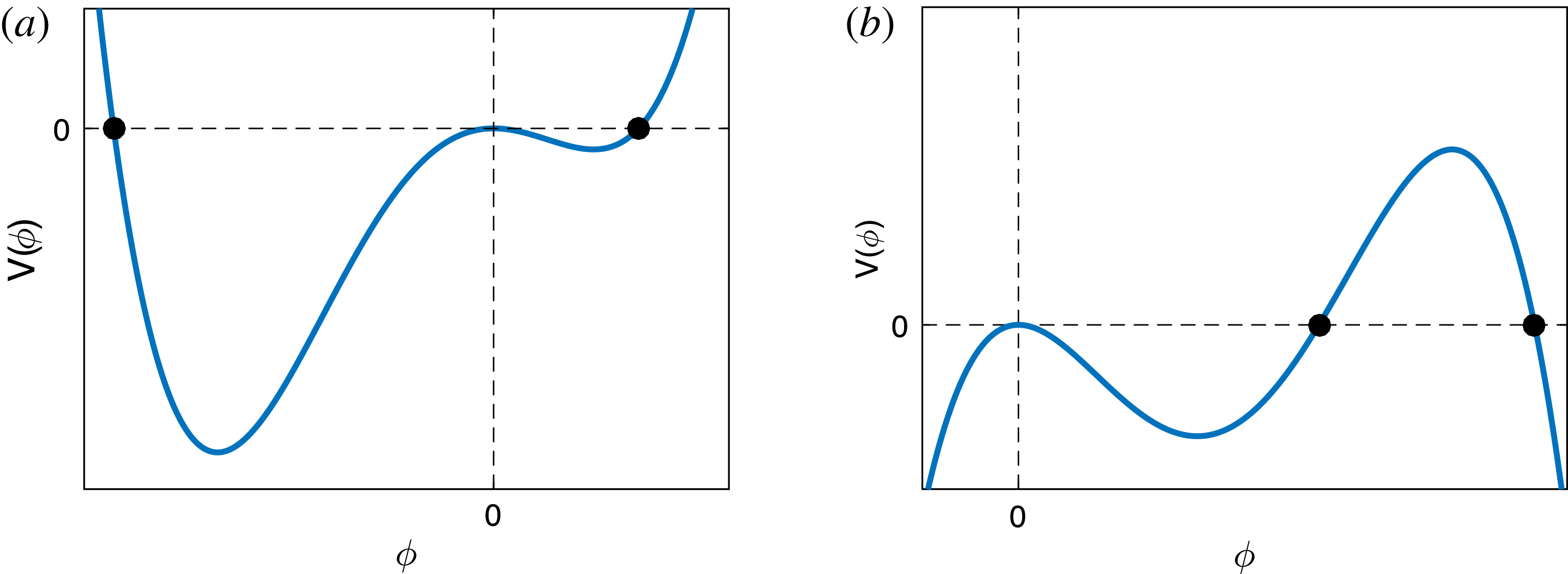
Typical Sagdeev potentials at near-critical compositions for
 $D_{0}>0$
(a) and
 $D_{0}<0$
(b). In both cases
 $\unicode[STIX]{x1D6FF}M>0$
and
 $C_{0}>0$
.

The sign of
 $D_{0}$
plays an important role in determining the characteristics of the resulting soliton(s). The difference is illustrated in figure 1. A typical Sagdeev potential for
 $D_{0}>0$
and
 $\unicode[STIX]{x1D6FF}M>0$
is shown in figure 1(a). Here we see that there are two roots, each corresponding to a soliton. The largest of the roots are given by the nonKdV-like branch. For
 $C_{0}>0$
(
 $C_{0}<0$
) this corresponds to the root
 $\unicode[STIX]{x1D719}_{r-}$
(
 $\unicode[STIX]{x1D719}_{r+}$
) in (2.23). On the other hand, figure 1(b) illustrates a typical Sagdeev potential when
 $D_{0}<0$
and
 $\unicode[STIX]{x1D6FF}M>0$
. Here we see two roots. However, only the smallest root corresponds to a soliton, since the equilibrium
 $\unicode[STIX]{x1D719}=0$
is not accessible from the larger root. For
 $C_{0}>0$
(
 $C_{0}<0$
) the soliton amplitude is given by the root
 $\unicode[STIX]{x1D719}_{r-}$
(
 $\unicode[STIX]{x1D719}_{r+}$
) in (2.23). Because of these qualitative differences, we consider the cases
 $D_{0}>0$
and
 $D_{0}<0$
separately.
To start off, we consider
 $D_{0}>0$
. Since
 $B_{1}D_{0}<0$
, it follows that the second term in the square root of (2.23) is positive. Therefore any choice of
 $\unicode[STIX]{x1D6FF}M>0$
will provide a positive contribution. However, the soliton amplitude increases when the choice of
 $\unicode[STIX]{x1D6FF}M$
is increased. We should therefore restrict ourselves to choices of
 $\unicode[STIX]{x1D6FF}M$
that ensures that
 $|\unicode[STIX]{x1D719}_{r}|\ll 1$
.
To quantify this restriction, we expand the amplitude as a Taylor series to obtain the following approximation:
 $$\begin{eqnarray}|\unicode[STIX]{x1D719}_{r}|\approx \left|\frac{-C_{0}^{2}\pm B_{1}D_{0}\unicode[STIX]{x1D6FF}M}{C_{0}D_{0}}\right|.\end{eqnarray}$$
It follows that the largest root (in absolute terms) satisfies
 $$\begin{eqnarray}\left|\frac{-C_{0}^{2}\pm B_{1}D_{0}\unicode[STIX]{x1D6FF}M}{C_{0}D_{0}}\right|=\left|\frac{C_{0}}{D_{0}}\right|+\left|\frac{B_{1}\unicode[STIX]{x1D6FF}M}{C_{0}}\right|.\end{eqnarray}$$
To ensure a small amplitude, one may require that the contribution of the second term on the right-hand side of (2.25) should not exceed the first term. This leads to the following criterion:
 $$\begin{eqnarray}\unicode[STIX]{x1D6FF}M\leqslant \left|\frac{C_{0}^{2}}{B_{1}D_{0}}\right|.\end{eqnarray}$$
We can see that this places a strong limitation on
 $\unicode[STIX]{x1D6FF}M$
due to the smallness of
 $C_{0}^{2}$
.
In the case where
 $D_{0}<0$
, the second term in the square root of (2.23) is negative since
 $B_{1}D_{0}>0$
. Therefore the amplitudes are bounded above by
 $\unicode[STIX]{x1D719}_{r}=|C_{0}/2D_{0}|$
. However, for the solution to be real, it follows that
 $$\begin{eqnarray}\unicode[STIX]{x1D6FF}M\leqslant \frac{C_{0}^{2}}{4B_{1}D_{0}}.\end{eqnarray}$$
3 Non-critical plasma compositions
We start our analysis of small-amplitude solitons with the most common scenario, namely a non-critical plasma composition where
 $|C_{0}|\gg |D_{0}\unicode[STIX]{x1D719}_{r}|$
. From (2.16) it follows that the Taylor series can be approximated as follows:
 $$\begin{eqnarray}V(\unicode[STIX]{x1D719},M)\approx B_{1}\unicode[STIX]{x1D6FF}M\unicode[STIX]{x1D719}^{2}+C_{0}\unicode[STIX]{x1D719}^{3},\end{eqnarray}$$
where
 $M=M_{0}+\unicode[STIX]{x1D6FF}M$
. To find an analytical solution, we substitute the approximate potential (3.1) into the energy-like integral (2.3). After simplifying the resulting equation, one obtains the following separable differential equation:
 $$\begin{eqnarray}\frac{\text{d}\unicode[STIX]{x1D719}}{\text{d}\unicode[STIX]{x1D709}}=\pm \sqrt{-2B_{1}\unicode[STIX]{x1D6FF}M}\left(\unicode[STIX]{x1D719}\sqrt{1+\frac{C_{0}}{B_{1}\unicode[STIX]{x1D6FF}M}\unicode[STIX]{x1D719}}\right).\end{eqnarray}$$
If we introduce the variable
 $\unicode[STIX]{x1D713}^{2}=-C_{0}\unicode[STIX]{x1D719}/B_{1}\unicode[STIX]{x1D6FF}M$
, then (3.2) can be written as
 $$\begin{eqnarray}-\frac{\text{d}\unicode[STIX]{x1D713}}{\unicode[STIX]{x1D713}\sqrt{1-\unicode[STIX]{x1D713}^{2}}}=\pm \sqrt{-\frac{B_{1}\unicode[STIX]{x1D6FF}M}{2}}\,\text{d}\unicode[STIX]{x1D709}.\end{eqnarray}$$
By integrating (3.3), and substituting back the original coordinates, one obtains the following soliton solution:
 $$\begin{eqnarray}\unicode[STIX]{x1D719}(x,t)=\frac{-B_{1}\unicode[STIX]{x1D6FF}M}{C_{0}}\text{sech}^{2}\left[\sqrt{\frac{-B_{1}\unicode[STIX]{x1D6FF}M}{2}}(x-x_{0}-Mt)\right],\end{eqnarray}$$
where
 $M=M_{0}+\unicode[STIX]{x1D6FF}M$
and
 $x_{0}$
is an arbitrary initial position of the soliton.
This solution agrees qualitatively with the KdV soliton solution obtained from the reductive perturbation method. However, in this case we see that the scalars
 $B_{1}$
and
 $C_{0}$
can be expressed in terms of derivatives of the Sagdeev potential. From § 2 we know that the solution is valid provided that
 $\unicode[STIX]{x1D6FF}M\ll |C_{0}/B_{1}|$
. Large values of
 $\unicode[STIX]{x1D6FF}M$
results in larger contributions from the truncated terms of the Taylor series expansion, so that the approximation breaks down.
4 Critical plasma compositions
Critical compositions in parameter space satisfy the condition
 $C_{0}=0$
. For such cases the Sagdeev potential can be written as follows:
 $$\begin{eqnarray}V(\unicode[STIX]{x1D719},M)\approx B_{1}\unicode[STIX]{x1D6FF}M\unicode[STIX]{x1D719}^{2}+D_{0}\unicode[STIX]{x1D719}^{4}.\end{eqnarray}$$
The results depend significantly on the sign of
 $D_{0}$
.
We start off by considering solitons at the acoustic speed
 $\unicode[STIX]{x1D6FF}M=0$
. Then the lowest-order approximation of the Sagdeev potential around
 $\unicode[STIX]{x1D719}=0$
and
 $M=M_{0}$
is given by
 $$\begin{eqnarray}V(\unicode[STIX]{x1D719},M_{0})\approx D_{0}\unicode[STIX]{x1D719}^{4}.\end{eqnarray}$$
When
 $D_{0}>0$
, it follows that the Sagdeev potential
 $V(\unicode[STIX]{x1D719},M_{0})$
is positive for
 $|\unicode[STIX]{x1D719}|\ll 1$
. This violates the existence conditions of solitons. From this one can conclude that no acoustic speed soliton of either small or large amplitude is possible at critical compositions satisfying
 $D_{0}>0$
.
On the other hand, when
 $D_{0}<0$
, we see that the Sagdeev potential is negative for
 $|\unicode[STIX]{x1D719}|\ll 1$
. Therefore, although there are no small-amplitude acoustic speed structures, the higher-order terms may result in large roots, corresponding to large-amplitude nonlinear structures. This has been reported by Olivier et al. (Reference Olivier, Maharaj and Bharuthram2015) for a plasma model consisting of two ion species and two Boltzmann electron species.
Next we consider the Sagdeev potential at a velocity that is slightly larger than the acoustic speed,
 $M=M_{0}+\unicode[STIX]{x1D6FF}M$
where
 $\unicode[STIX]{x1D6FF}M\ll 1$
. In this case the lowest-order approximation of the Sagdeev potential is given by (4.1). It is clear that the Sagdeev potential is symmetric in
 $\unicode[STIX]{x1D719}$
. This means that small-amplitude soliton solutions arise in symmetric pairs.
To show this, we use the Sagdeev potential (4.1) to obtain exact expressions for the soliton solutions associated with critical compositions. By substituting the Sagdeev potential (4.1) into the energy integral (2.3), one obtains the following separable equation:
 $$\begin{eqnarray}\frac{\text{d}\unicode[STIX]{x1D719}}{\text{d}\unicode[STIX]{x1D709}}=\pm \sqrt{-2B_{1}\unicode[STIX]{x1D6FF}M}\unicode[STIX]{x1D719}\sqrt{1+\frac{D_{0}}{B_{1}\unicode[STIX]{x1D6FF}M}\unicode[STIX]{x1D719}^{2}}.\end{eqnarray}$$
By making the substitution
 $\unicode[STIX]{x1D713}=\sqrt{-B_{1}\unicode[STIX]{x1D6FF}M/D_{0}}/\unicode[STIX]{x1D719}$
, the separable equation (4.3) can be written in the form
 $$\begin{eqnarray}\frac{\text{d}\unicode[STIX]{x1D713}}{\sqrt{\unicode[STIX]{x1D713}^{2}-1}}=\pm \sqrt{-2B_{1}\unicode[STIX]{x1D6FF}M}\,\text{d}\unicode[STIX]{x1D709}.\end{eqnarray}$$
By integrating (4.4), and substituting the original coordinates, one obtains the following soliton solutions:
 $$\begin{eqnarray}\unicode[STIX]{x1D719}(x,t)=\pm \sqrt{\frac{-B_{1}\unicode[STIX]{x1D6FF}M}{D_{0}}}\text{sech}\left[\sqrt{-2B_{1}\unicode[STIX]{x1D6FF}M}(x-x_{0}-Mt)\right],\end{eqnarray}$$
where
 $M=M_{0}+\unicode[STIX]{x1D6FF}M$
and
 $x_{0}$
is an arbitrary initial position of the soliton. From the condition (2.20) we know that the solution is only valid provided that
 $\sqrt{-B_{1}\unicode[STIX]{x1D6FF}M/D_{0}}\ll 1$
.
Since
 $B_{1}<0$
, it follows that the solution is only real when
 $D_{0}>0$
. In this case one obtains two small-amplitude soliton solutions with opposite polarity. This means that coexistence of a positive and a negative polarity soliton occur at critical compositions in parameter space when
 $D_{0}>0$
. This agrees well with reductive perturbation analysis where the mKdV equation is derived. On the other hand, no small-amplitude solitons arise for critical compositions where
 $D_{0}<0$
.
Based on these findings, we can conclude that there are two types of critical compositions, depending on the sign of
 $D_{0}$
. We distinguish between the two types by referring to critical compositions satisfying
 $D_{0}>0$
as rich critical compositions and critical compositions with
 $D_{0}<0$
as poor critical compositions.
It should be noted that the coexistence at rich critical compositions does not involve a large-amplitude acoustic speed soliton, but arises in the form of two KdV-like families of solutions that both vanish in the acoustic speed limit. These results agree qualitatively with reductive perturbation theory, where the mKdV equation governs small-amplitude soliton solutions. This result is also consistent with recent studies where the fully nonlinear Sagdeev potential was applied (Olivier et al. Reference Olivier, Maharaj and Bharuthram2015; Mbuli et al. Reference Mbuli, Maharaj, Bharuthram, Singh and Lakhina2016).
5 Near-critical plasma compositions
A useful extension of the analysis of critical compositions is to consider the effect of a small deviation from a critical plasma composition. This allows us to consider near-critical compositions. Such a deviation would result in small changes in the coefficients of the Sagdeev potential, and will usually result in a small but finite value of
 $C_{0}$
. We can use this fact to establish the soliton properties in the vicinity of a critical plasma composition.
To this end, we consider a near-critical plasma composition that satisfies the relation
 $|C_{0}\unicode[STIX]{x1D719}_{r}^{3}|\sim |D_{0}\unicode[STIX]{x1D719}_{r}^{4}|$
. At the near-critical composition, one can express the Sagdeev potential as a truncated Taylor series as shown in (2.22), given by
 $$\begin{eqnarray}V(\unicode[STIX]{x1D719},M)=B_{1}\unicode[STIX]{x1D6FF}M\unicode[STIX]{x1D719}^{2}+C_{0}\unicode[STIX]{x1D719}^{3}+D_{0}\unicode[STIX]{x1D719}^{4}.\end{eqnarray}$$
Substitution of the potential (5.1) into the energy integral (2.3) and simplification lead to the following separable equation:
 $$\begin{eqnarray}\frac{\text{d}\unicode[STIX]{x1D719}}{\text{d}\unicode[STIX]{x1D709}}=\pm \sqrt{-2B_{1}\unicode[STIX]{x1D6FF}M}\unicode[STIX]{x1D719}\sqrt{1+\frac{C_{0}}{B_{1}\unicode[STIX]{x1D6FF}M}\unicode[STIX]{x1D719}+\frac{D_{0}}{B_{1}\unicode[STIX]{x1D6FF}M}\unicode[STIX]{x1D719}^{2}}.\end{eqnarray}$$
The substitution
 $\unicode[STIX]{x1D713}=1/\unicode[STIX]{x1D719}+C_{0}/2B_{1}\unicode[STIX]{x1D6FF}M$
leads to an equation of the form
 $$\begin{eqnarray}\frac{\text{d}\unicode[STIX]{x1D713}}{\sqrt{\unicode[STIX]{x1D713}^{2}-\displaystyle \frac{C_{0}^{2}-4B_{1}D_{0}\unicode[STIX]{x1D6FF}M}{4B_{1}^{2}\unicode[STIX]{x1D6FF}M^{2}}}}=\pm \sqrt{-2B_{1}\unicode[STIX]{x1D6FF}M}\,\text{d}\unicode[STIX]{x1D709}.\end{eqnarray}$$
By integrating the equation, and substituting back the original coordinates, one obtains the following solutions:
 $$\begin{eqnarray}\unicode[STIX]{x1D719}(x,t)=\frac{-2B_{1}\unicode[STIX]{x1D6FF}M}{C_{0}\pm \sqrt{C_{0}^{2}-4B_{1}D_{0}\unicode[STIX]{x1D6FF}M}\text{cosh}\left[\sqrt{-2B_{1}\unicode[STIX]{x1D6FF}M}(x-x_{0}-Mt)\right]},\end{eqnarray}$$
where
 $M=M_{0}+\unicode[STIX]{x1D6FF}M$
and
 $x_{0}$
is the arbitrary initial position of the soliton.
The choice of
 $\pm$
depends on the sign of
 $D_{0}$
. We therefore make the following distinction between two types of near-critical compositions. In keeping with § 4, we refer to a near-critical composition with
 $D_{0}>0$
(
 $D_{0}<0$
) as a rich (poor) near-critical composition. We now consider the two cases separately.
5.1 Rich near-critical compositions
 $(D_{0}>0)$

Consider a rich near-critical composition where
 $D_{0}>0$
. From (5.4) it follows that the solution is real whenever
 $C_{0}^{2}-4B_{1}D_{0}\unicode[STIX]{x1D6FF}M>0$
. This condition is met whenever
 $\unicode[STIX]{x1D6FF}M>0$
due to the fact that
 $B_{1}D_{0}<0$
. When
 $C_{0}>0$
(
 $C_{0}<0$
), the upper plus sign (lower minus sign) corresponds to a KdV-like family of soliton solutions, while the lower minus sign (upper plus sign) corresponds to a nonKdV-like family of soliton solutions. These solutions are in good agreement with those obtained from reductive perturbation analysis, where the small-amplitude solitons are governed by the Gardner equation. From § 2 we also know that the solution is a reasonable approximation provided that
 $\unicode[STIX]{x1D6FF}M\leqslant |C_{0}^{2}/2B_{1}D_{0}|$
.
The solutions obtained above show that coexistence does not only arise at rich critical compositions, but also at rich near-critical compositions. In terms of the compositional parameter space, one may therefore think of rich critical compositions as sources of coexistence.
We now proceed to derive a novel analytical solution of the acoustic speed soliton at rich near-critical compositions. At the acoustic speed, the Sagdeev potential in the vicinity of
 $\unicode[STIX]{x1D719}=0$
can be approximated by
 $$\begin{eqnarray}V(\unicode[STIX]{x1D719},M_{0})\approx C_{0}\unicode[STIX]{x1D719}^{3}+D_{0}\unicode[STIX]{x1D719}^{4}.\end{eqnarray}$$
If we substitute this expression into the energy integral (2.3), the equation can be written as a separable differential equation of the form
 $$\begin{eqnarray}\frac{\text{d}\unicode[STIX]{x1D719}}{\unicode[STIX]{x1D719}\sqrt{-C_{0}\unicode[STIX]{x1D719}-D_{0}\unicode[STIX]{x1D719}^{2}}}=\pm \sqrt{2}\,\text{d}\unicode[STIX]{x1D709}.\end{eqnarray}$$
The equation can be integrated by using the identity
 $$\begin{eqnarray}\int \frac{\text{d}x}{x\sqrt{ax^{2}+bx}}=-\frac{2\sqrt{ax^{2}+bx}}{bx}+\text{constant}.\end{eqnarray}$$
After simplification, one obtains the following acoustic speed soliton solution:
 $$\begin{eqnarray}\unicode[STIX]{x1D719}(x,t)=-\frac{C_{0}}{D_{0}+{\textstyle \frac{1}{2}}C_{0}^{2}(x-x_{0}-M_{0}t)^{2}},\end{eqnarray}$$
where
 $x_{0}$
is the arbitrary initial position of the solution and
 $M_{0}$
is the relevant acoustic speed. To the best of our knowledge, no analytical expression of an acoustic speed soliton has been reported to date.
It is important to note that the acoustic speed soliton solution (5.8) is a Lorentzian pulse. Unlike the other soliton solutions, it does not decay exponentially fast. Indeed, as
 $|x|\rightarrow \infty$
, we see that
 $\unicode[STIX]{x1D719}\rightarrow -2/C_{0}x^{2}$
. This means that the decay rate is much slower than the sech-type soliton solutions that decay exponentially fast.
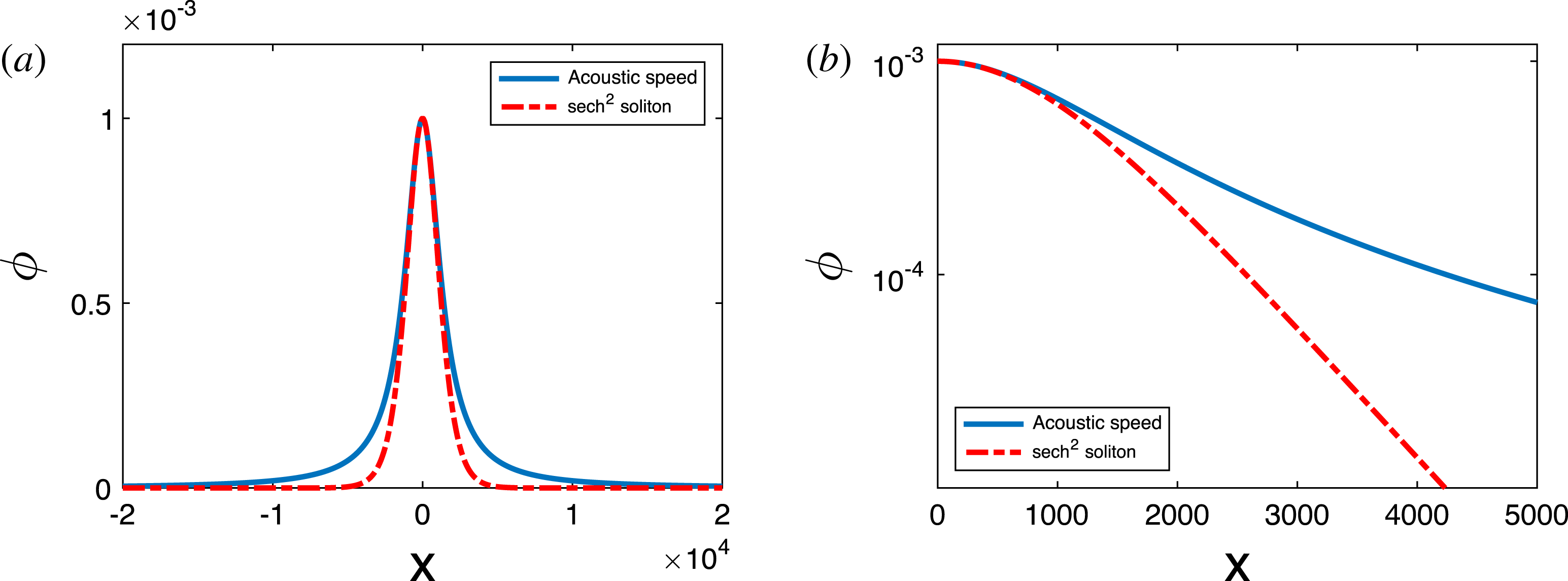
To illustrate the difference between acoustic speed solitons and regular solitons, we compare two solutions with equal amplitude. The first is the acoustic speed soliton solution (5.8) where
 $C_{0}=-10^{-3}$
and
 $D_{0}=1$
. The second is the
 $\text{sech}^{2}$
soliton solution (3.4). Here we want to choose coefficients in such a way that both solutions have the same amplitude and similar profiles near the peak. To achieve this, we require that the second derivatives must be equal at
 $\unicode[STIX]{x1D719}=0$
. This can be achieved by choosing
 $\unicode[STIX]{x1D6FF}M=10^{-3}$
and
 $C_{0}=-B_{1}=10^{3}$
. In both cases we set
 $t=x_{0}=0$
.
Comparison of the acoustic speed soliton (solid line) and the regular
 $\text{sech}^{2}$
soliton (dashed line). In (a) the
 $\unicode[STIX]{x1D719}$
-axis applies a linear scale, while the
 $\unicode[STIX]{x1D719}$
-axis in (b) applies a logarithmic scale.

The results are shown in figure 2, where the solid lines correspond to the acoustic speed soliton, and the dotted lines correspond to the regular soliton. In figure 2(a) we can see that the solutions are similar on the interval
 $-1000\leqslant x\leqslant 1000$
. However, the acoustic speed soliton has much fatter tails. In figure 2(b) we plot the tails on the right hand side of the solutions by using a logarithmic scale for the
 $\unicode[STIX]{x1D719}$
-axis. Here we see that the regular soliton solution decreases linearly due to its exponential rate of decay. However, the decaying rate of the acoustic speed soliton tapers off at larger values of
 $x$
. This clearly illustrates the difference between the exponential decreasing rate of regular solitons and the algebraic decreasing rate of Lorentzian acoustic speed solitons.
5.2 Poor near-critical compositions
$(D_{0}<0)$

To analyse the significance of a poor critical composition in parameter space, consider a poor near-critical composition where
 $D_{0}<0$
. From the soliton solutions (5.4), it follows that the solution is real whenever
 $$\begin{eqnarray}\unicode[STIX]{x1D6FF}M\leqslant C_{0}^{2}/4B_{1}D_{0}.\end{eqnarray}$$
Also, the choice of the
 $\pm$
sign must be chosen in such a way that the denominator remains non-zero for all choices of
 $x$
and
 $t$
. This is achieved by choosing the same sign as
 $C_{0}$
. In other words, we choose the upper positive sign (lower negative sign) when
 $C_{0}>0$
 $(C_{0}<0)$
. This shows that only one of the solutions (5.4) is valid. This is consistent with our analysis in § 2.
It is important to note that this rules out the coexistence of two small-amplitude solitons. However, there may be large-amplitude nonKdV-like solitons that are inaccessible via our analysis. In short, poor near-critical compositions neither implies nor rules out coexistence.
At the critical velocity
 $\unicode[STIX]{x1D6FF}M_{DL}=C_{0}^{2}/4B_{1}D_{0}$
, the solution (5.4) is no longer valid. In this case the Sagdeev potential has a double root at
 $\unicode[STIX]{x1D719}_{r}=-C_{0}/2D_{0}$
, and can be written as
 $$\begin{eqnarray}V(\unicode[STIX]{x1D719},M_{DL})\approx -\unicode[STIX]{x1D719}^{2}\left(\sqrt{-D_{0}}\unicode[STIX]{x1D719}-\frac{C_{0}}{2\sqrt{-D_{0}}}\right)^{2},\end{eqnarray}$$
where
 $M_{DL}=M_{0}+\unicode[STIX]{x1D6FF}M_{DL}$
. If we substitute this potential into the energy integral (2.3), one obtains the following separable equation:
 $$\begin{eqnarray}\frac{\text{d}\unicode[STIX]{x1D719}}{\text{d}\unicode[STIX]{x1D709}}=\pm \sqrt{-2D_{0}}\left(\unicode[STIX]{x1D719}^{2}+\frac{C_{0}}{2D_{0}}\unicode[STIX]{x1D719}\right).\end{eqnarray}$$
One can rewrite the separable equation by completing the square in the bracketed term, and making the transformation
 $\unicode[STIX]{x1D713}=-4D_{0}\unicode[STIX]{x1D719}/C_{0}-1$
. The separable equation (5.11) then becomes
 $$\begin{eqnarray}\frac{\text{d}\unicode[STIX]{x1D713}}{1-\unicode[STIX]{x1D713}^{2}}=\pm \sqrt{-\frac{C_{0}^{2}}{8D_{0}}}\,\text{d}\unicode[STIX]{x1D709}.\end{eqnarray}$$
By integrating the equation, ensuring that the solution satisfies the boundary conditions, and substituting back the original coordinates, one obtains the following double layer solution:
 $$\begin{eqnarray}\unicode[STIX]{x1D719}(x,t)=-\frac{C_{0}}{4D_{0}}\left\{1-\text{tanh}\left[\sqrt{-\frac{C_{0}^{2}}{8D_{0}}}(x-x_{0}-M_{DL}t)\right]\right\}.\end{eqnarray}$$
Here
 $M_{DL}=C_{0}^{2}/4B_{1}D_{0}$
and
 $x_{0}$
is an arbitrary initial position of the double layer. This solution is consistent with reductive perturbation theory, where small-amplitude double layer solutions are governed by the Gardner equation.
These results show that weak double layer solutions are found near poor critical compositions. Therefore poor critical compositions act as sources of weak double layers in the compositional parameter space.
6 Case study: simple model with cold ions and two-temperature electrons
We present a simple case study that allows us to illustrate all the main features of the results obtained above. This is done by considering a well-studied plasma model consisting of a cold fluid ion species and a two-temperature Boltzmann electron species. We also use the model to compare the small-amplitude solitons to those obtained from reductive perturbation theory.
The normalized fluid equations consist of the equations of continuity, momentum, and Poisson’s equation, given by Verheest, Olivier & Hereman (Reference Verheest, Olivier and Hereman2016) as
 $$\begin{eqnarray}\displaystyle & \displaystyle \frac{\unicode[STIX]{x2202}n}{\unicode[STIX]{x2202}t}+\frac{\unicode[STIX]{x2202}}{\unicode[STIX]{x2202}x}(nv)=0, & \displaystyle\end{eqnarray}$$
 $$\begin{eqnarray}\displaystyle & \displaystyle \frac{\unicode[STIX]{x2202}v}{\unicode[STIX]{x2202}t}+v\frac{\unicode[STIX]{x2202}v}{\unicode[STIX]{x2202}x}+\frac{\unicode[STIX]{x2202}\unicode[STIX]{x1D719}}{\unicode[STIX]{x2202}x}=0, & \displaystyle\end{eqnarray}$$
 $$\begin{eqnarray}\displaystyle & \displaystyle \frac{\unicode[STIX]{x2202}^{2}\unicode[STIX]{x1D719}}{\unicode[STIX]{x2202}x^{2}}+n-f\exp (\unicode[STIX]{x1D6FC}_{c}\unicode[STIX]{x1D719})-(1-f)\exp (\unicode[STIX]{x1D6FC}_{h}\unicode[STIX]{x1D719})=0, & \displaystyle\end{eqnarray}$$
respectively. In the fluid equations
 $n$
denotes the ion number density normalized with respect to the equilibrium ion density
 $N_{i}$
while
 $v$
denotes the fluid velocity normalized with respect to the ion-acoustic speed
 $c_{ia}=\sqrt{K_{B}T_{eff}/m_{i}}$
with ion mass
 $m_{i}$
. Here
 $K_{B}$
denotes the Boltzmann constant and
 $T_{eff}=T_{c}/[f+(1-f)\unicode[STIX]{x1D70F}]$
denotes the effective temperature with electron temperature ratio
 $\unicode[STIX]{x1D70F}=T_{c}/T_{h}$
for cool (hot) electron temperature
 $T_{c}$
 $(T_{h})$
. The equilibrium cool electron density
 $f$
is normalized with respect to
 $N_{i}$
. In addition
 $\unicode[STIX]{x1D719}$
denotes the electrostatic potential normalized with respect to
 $K_{B}T_{eff}/e$
where
 $e$
denotes the electron charge, while
 $\unicode[STIX]{x1D6FC}_{c}=T_{eff}/T_{c}$
and
 $\unicode[STIX]{x1D6FC}_{h}=T_{eff}/T_{h}$
. Finally lengths
 $x$
and time
 $t$
are normalized with respect to
 $\unicode[STIX]{x1D706}_{D}=\sqrt{\unicode[STIX]{x1D700}_{0}\unicode[STIX]{x1D705}T_{eff}/(N_{i}e^{2})}$
and
 $\unicode[STIX]{x1D714}_{pi}^{-1}=\sqrt{\unicode[STIX]{x1D700}_{0}m_{i}/N_{i}e^{2}}$
, respectively.
Baluku et al. (Reference Baluku, Hellberg and Verheest2010) showed that critical compositions only arise for electron temperature ratios
 $\unicode[STIX]{x1D70F}<\unicode[STIX]{x1D70F}_{c}$
, where
 $\unicode[STIX]{x1D70F}_{c}=5-2\sqrt{6}\approx 0.10102$
. In order to retain only one degree of freedom
 $(f)$
while ensuring critical densities, we fix the electron temperature ratio
 $\unicode[STIX]{x1D70F}=0.1$
. For this temperature ratio the Sagdeev potential is given by Baluku et al. (Reference Baluku, Hellberg and Verheest2010):
 $$\begin{eqnarray}V(\unicode[STIX]{x1D719},M)=M^{2}[1-(1-2\unicode[STIX]{x1D719}/M^{2})^{1/2}]+\frac{f}{\unicode[STIX]{x1D6FC}_{c}}[1-\exp (\unicode[STIX]{x1D6FC}_{c}\unicode[STIX]{x1D719})]+\frac{1-f}{\unicode[STIX]{x1D6FC}_{h}}[1-\exp (\unicode[STIX]{x1D6FC}_{h}\unicode[STIX]{x1D719})],\end{eqnarray}$$
where
 $\unicode[STIX]{x1D6FC}_{c}=10/(1+9f)$
and
 $\unicode[STIX]{x1D6FC}_{h}=1/(1+9f)$
.
We now proceed to derive the small-amplitude soliton and double layer solutions using our Sagdeev potential analysis.
6.1 Sagdeev analysis
Differentiation of the Sagdeev potential (6.4) shows that
 $$\begin{eqnarray}B_{1}=-1,\quad C_{0}=\frac{3-A_{2}}{6},\quad D_{0}=\frac{15-A_{3}}{24},\end{eqnarray}$$
where
 $$\begin{eqnarray}A_{2}=(1+99f)/(1+9f)^{2},\quad A_{3}=(1+999f)/(1+9f)^{3}.\end{eqnarray}$$
Critical compositions correspond to densities
 $f$
where the coefficient
 $C_{0}$
vanishes. It follows that there are two critical densities (Baluku et al.
Reference Baluku, Hellberg and Verheest2010):
 $$\begin{eqnarray}f_{p}=2/27\approx 0.074\end{eqnarray}$$
and
 $$\begin{eqnarray}f_{r}=1/9\approx 0.111.\end{eqnarray}$$
At
 $f_{p}$
and
 $f_{r}$
one finds that
 $D_{0}=-1/20$
and
 $D_{0}=1/24$
, respectively. Therefore
 $f_{p}$
and
 $f_{r}$
correspond to a poor critical composition and a rich critical composition, respectively.
6.1.1 Poor critical composition
$f_{p}$

We first consider
 $f_{p}$
. Since
 $D_{0}<0$
, the analysis shows that no small-amplitude soliton solutions arise.
It should be noted, however, that the Sagdeev potential has a root
 $\unicode[STIX]{x1D719}_{r}\approx 0.19417$
at the acoustic speed. This corresponds to a large-amplitude acoustic speed soliton. This large-amplitude soliton gives rise to a family of nonKdV-like solitons. This serves as a reminder that the results obtained from our analysis only apply to the small-amplitude regime. Since this paper is concerned with small-amplitude solitons, we do not consider these soliton solutions in more detail.
We now consider near-critical densities that are slightly larger than the critical density
 $f=f_{p}+\unicode[STIX]{x1D6FF}f$
, where
 $\unicode[STIX]{x1D6FF}f\ll 1$
. From (6.5) we get that
 $A_{2}\approx 3+81\unicode[STIX]{x1D6FF}f/25$
and that
 $A_{3}\approx 81/5-(5832/125)\unicode[STIX]{x1D6FF}M$
so that
 $$\begin{eqnarray}C_{0}\approx -27\unicode[STIX]{x1D6FF}f/50,\quad D_{0}\approx -1/20+243\unicode[STIX]{x1D6FF}f/125.\end{eqnarray}$$
It follows that the upper plus sign of solution (5.4) applies. We therefore get the following family of soliton solutions:
 $$\begin{eqnarray}\unicode[STIX]{x1D719}(x,t)=\frac{100\unicode[STIX]{x1D6FF}M}{-27\unicode[STIX]{x1D6FF}f+\sqrt{729\unicode[STIX]{x1D6FF}f^{2}-(500-19440\unicode[STIX]{x1D6FF}f)\unicode[STIX]{x1D6FF}M}\text{cosh}\left[\sqrt{2\unicode[STIX]{x1D6FF}M}(x-Mt)\right]},\end{eqnarray}$$
where
 $M=1+\unicode[STIX]{x1D6FF}M$
. From (5.9) it follows that the solution is valid whenever
 $$\begin{eqnarray}\unicode[STIX]{x1D6FF}M<\frac{729\unicode[STIX]{x1D6FF}f^{2}}{500-19440\unicode[STIX]{x1D6FF}f}.\end{eqnarray}$$
Equation (5.13) shows that the double layer solution is given by
 $$\begin{eqnarray}\unicode[STIX]{x1D719}(x,t)=-\frac{270\unicode[STIX]{x1D6FF}f}{25-972\unicode[STIX]{x1D6FF}f}\left\{1-\text{tanh}\left[\frac{1}{50}\sqrt{729\unicode[STIX]{x1D6FF}f^{2}-(500-19440\unicode[STIX]{x1D6FF}f)\unicode[STIX]{x1D6FF}M}(x-M_{DL}t)\right]\right\},\end{eqnarray}$$
where
 $M_{DL}=1+729\unicode[STIX]{x1D6FF}f^{2}/(500-19440\unicode[STIX]{x1D6FF}f)$
.
6.1.2 Rich critical composition
$f_{r}$

At the critical density
 $f_{r}=1/9$
, we find that
 $D_{0}=1/24$
. The analysis predicts the existence of both positive and negative polarity solitons. From (4.5) it follows that the solutions are given by
 $$\begin{eqnarray}\unicode[STIX]{x1D719}(x,t)=\pm \sqrt{24\unicode[STIX]{x1D6FF}M}\text{sech}\left[\sqrt{2\unicode[STIX]{x1D6FF}M}(x-Mt)\right],\end{eqnarray}$$
where
 $M=1+\unicode[STIX]{x1D6FF}M$
. This solution is valid provided that
 $\unicode[STIX]{x1D6FF}M\ll 1$
.
We next consider rich near-critical compositions that are slightly larger than the critical density
 $f=f_{r}+\unicode[STIX]{x1D6FF}f$
, where
 $\unicode[STIX]{x1D6FF}f\ll 1$
. From (6.6) one can show that
 $A_{2}\approx 3-9\unicode[STIX]{x1D6FF}f/4$
and
 $A_{3}\approx 14+831\unicode[STIX]{x1D6FF}f/8$
. If we substitute these values into (6.5) one obtains
 $$\begin{eqnarray}C_{0}\approx 3\unicode[STIX]{x1D6FF}f/8,\quad D_{0}\approx 1/24+171\unicode[STIX]{x1D6FF}f/64.\end{eqnarray}$$
The soliton solutions of the near-critical compositions are given by (5.4). Substituting the values of
 $C_{0}$
and
 $D_{0}$
(6.14) into this solution we obtain the following two families of soliton solutions:
 $$\begin{eqnarray}\unicode[STIX]{x1D719}(x,t)=\frac{48\unicode[STIX]{x1D6FF}M}{9\unicode[STIX]{x1D6FF}f\pm \sqrt{81\unicode[STIX]{x1D6FF}f^{2}+(96+2052\unicode[STIX]{x1D6FF}f)\unicode[STIX]{x1D6FF}M}\text{cosh}\left[\sqrt{2\unicode[STIX]{x1D6FF}M}(x-x_{0}-Mt)\right]},\end{eqnarray}$$
where
 $M=1+\unicode[STIX]{x1D6FF}M$
and
 $x_{0}$
is an arbitrary initial position of the soliton. Since
 $C_{0}>0$
it follows that the solution corresponding to the upper plus sign gives rise to positive polarity KdV-like solitons, while the lower minus sign gives rise to negative polarity nonKdV-like solitons. From the solution (5.8) it follows that a negative polarity acoustic speed soliton solution is given by
 $$\begin{eqnarray}\unicode[STIX]{x1D719}(x,t)=-\frac{144\unicode[STIX]{x1D6FF}f}{16+1026\unicode[STIX]{x1D6FF}f+27\unicode[STIX]{x1D6FF}f^{2}(x-x_{0}-t)^{2}}.\end{eqnarray}$$
6.2 Reductive perturbation analysis
We now apply reductive perturbation theory to the same model. We introduce the stretching coordinates
 $$\begin{eqnarray}\unicode[STIX]{x1D709}=\unicode[STIX]{x1D700}(x-t)\quad \text{and}\quad \unicode[STIX]{x1D70F}=\unicode[STIX]{x1D700}^{3}t.\end{eqnarray}$$
Here we use
 $\unicode[STIX]{x1D700}$
as a bookkeeping parameter in order to separate different orders of magnitude. We expand the ion number density
 $n$
, the fluid velocity
 $v$
and the electrostatic potential
 $\unicode[STIX]{x1D719}$
as follows:
 $$\begin{eqnarray}\displaystyle & \displaystyle n=1+\unicode[STIX]{x1D700}n_{1}+\unicode[STIX]{x1D700}^{2}n_{2}+\unicode[STIX]{x1D700}^{3}n_{3}+\cdots \,, & \displaystyle\end{eqnarray}$$
 $$\begin{eqnarray}\displaystyle & \displaystyle v=\unicode[STIX]{x1D700}v_{1}+\unicode[STIX]{x1D700}^{2}v_{2}+\unicode[STIX]{x1D700}^{3}v_{3}+\cdots \,, & \displaystyle\end{eqnarray}$$
 $$\begin{eqnarray}\displaystyle & \displaystyle \unicode[STIX]{x1D719}=\unicode[STIX]{x1D700}\unicode[STIX]{x1D719}_{1}+\unicode[STIX]{x1D700}^{2}\unicode[STIX]{x1D719}_{2}+\unicode[STIX]{x1D700}^{3}\unicode[STIX]{x1D719}_{3}\cdots \,. & \displaystyle\end{eqnarray}$$
 $$\begin{eqnarray}n_{1}=v_{1}=\unicode[STIX]{x1D719}_{1}.\end{eqnarray}$$
From Poisson’s equation (6.3), one obtains the compatibility condition
 $$\begin{eqnarray}(1-A_{1})\unicode[STIX]{x1D719}_{1}=0,\end{eqnarray}$$
where
 $$\begin{eqnarray}A_{1}=f\unicode[STIX]{x1D6FC}_{c}+(1-f)\unicode[STIX]{x1D6FC}_{h}=1,\end{eqnarray}$$
so that the compatibility condition (6.20) is satisfied.
At the second order, the equations of continuity (6.1) and momentum (6.2) give
 $$\begin{eqnarray}n_{2}=\unicode[STIX]{x1D719}_{2}+{\textstyle \frac{3}{2}}\unicode[STIX]{x1D719}_{1}^{2},\quad v_{2}=\unicode[STIX]{x1D719}_{2}+{\textstyle \frac{1}{2}}\unicode[STIX]{x1D719}_{1}^{2}\end{eqnarray}$$
while the following compatibility condition follows from Poisson’s equation (6.3):
 $$\begin{eqnarray}(1-A_{1})\unicode[STIX]{x1D719}_{2}+\frac{3-A_{2}}{2}\unicode[STIX]{x1D719}_{1}^{2}=0,\end{eqnarray}$$
where
 $A_{1}$
and
 $A_{2}$
are defined in (6.21) and (6.6), respectively. This condition is satisfied when
 $A_{2}=3$
. However, for near-critical compositions satisfying
 $(3-A_{2})/2\sim O(\unicode[STIX]{x1D700})$
, the second term in the compatibility condition (6.23) is relegated to the third order of Poisson’s equation (6.3), as its contribution is negligible on second-order scales.
Moving to the third-order equations, one can solve the contributions from the equations of continuity (6.1) and momentum (6.2), so that
 $\unicode[STIX]{x2202}n_{3}/\unicode[STIX]{x2202}\unicode[STIX]{x1D709}$
and
 $\unicode[STIX]{x2202}v_{3}/\unicode[STIX]{x2202}\unicode[STIX]{x1D709}$
can be expressed in terms of
 $\unicode[STIX]{x1D719}_{1}$
,
 $\unicode[STIX]{x1D719}_{2}$
and
 $\unicode[STIX]{x1D719}_{3}$
only. Here we retained the near-critical contribution
 $(1/2)(3-A_{2})\unicode[STIX]{x1D719}_{1}^{2}$
in the third-order Poisson’s equation (6.3). After substitution into Poisson’s equation and differentiation one obtains the Gardner equation
 $$\begin{eqnarray}\frac{\unicode[STIX]{x2202}\unicode[STIX]{x1D719}_{1}}{\unicode[STIX]{x2202}\unicode[STIX]{x1D70F}}+\frac{1}{2}\frac{\unicode[STIX]{x2202}^{3}\unicode[STIX]{x1D719}_{1}}{\unicode[STIX]{x2202}\unicode[STIX]{x1D709}^{3}}+a\unicode[STIX]{x1D719}_{1}\frac{\unicode[STIX]{x2202}\unicode[STIX]{x1D719}_{1}}{\unicode[STIX]{x2202}\unicode[STIX]{x1D709}}+b\unicode[STIX]{x1D719}_{1}^{2}\frac{\unicode[STIX]{x2202}\unicode[STIX]{x1D719}_{1}}{\unicode[STIX]{x2202}\unicode[STIX]{x1D709}}=0.\end{eqnarray}$$
Here
 $$\begin{eqnarray}a=\frac{3-A_{2}}{2},\quad b=\frac{15-A_{3}}{4},\end{eqnarray}$$
where
 $A_{2}$
and
 $A_{3}$
are defined in (6.6). A comparison between (6.5) and (6.25) shows that
 $$\begin{eqnarray}a=3C_{0},\quad b=6D_{0}.\end{eqnarray}$$
At the critical densities
 $f_{p}$
and
 $f_{r}$
, one finds that
 $a=0$
, so that the equation reduces to the mKdV equation, given by
 $$\begin{eqnarray}\frac{\unicode[STIX]{x2202}\unicode[STIX]{x1D719}_{1}}{\unicode[STIX]{x2202}\unicode[STIX]{x1D70F}}+\frac{1}{2}\frac{\unicode[STIX]{x2202}^{3}\unicode[STIX]{x1D719}_{1}}{\unicode[STIX]{x2202}\unicode[STIX]{x1D709}^{3}}+b\unicode[STIX]{x1D719}_{1}^{2}\frac{\unicode[STIX]{x2202}\unicode[STIX]{x1D719}_{1}}{\unicode[STIX]{x2202}\unicode[STIX]{x1D709}}=0.\end{eqnarray}$$
The Gardner and mKdV equations are integrable, and their solutions depend on the sign of the cubic nonlinear coefficient
 $b$
.
We now proceed to consider small-amplitude solutions at and near the two critical densities
 $f_{p}$
and
 $f_{r}$
.
6.2.1 Poor critical composition
$f_{p}$

At the critical density
 $f_{p}=2/27$
we get the mKdV equation (6.27) with
 $a=0$
and
 $b=-0.3$
. When
 $b<0$
, the mKdV equation has no soliton solutions that satisfies the boundary conditions. This is in agreement with our Sagdeev analysis.
The Gardner equation (6.24) has well-known soliton solutions given by
 $$\begin{eqnarray}\unicode[STIX]{x1D719}_{1}(\unicode[STIX]{x1D709},\unicode[STIX]{x1D70F})=\frac{6U}{a\pm (a^{2}+6Ub)^{1/2}\text{cosh}\left[\sqrt{2U}(\unicode[STIX]{x1D709}-U\unicode[STIX]{x1D70F})\right]}.\end{eqnarray}$$
For
 $b<0$
, the upper plus (lower minus) sign is chosen for
 $a>0$
 $(a<0)$
. At near-critical densities
 $f=f_{p}+\unicode[STIX]{x1D6FF}f$
, we get that
 $A_{2}\approx 3+81\unicode[STIX]{x1D6FF}f/25$
so that
 $a\approx -81\unicode[STIX]{x1D6FF}f/50$
. Therefore the lower minus sign of the solution (6.28) applies. Finally, by setting
 $\unicode[STIX]{x1D700}=1$
,
 $U=\unicode[STIX]{x1D6FF}M$
and expressing
 $a$
and
 $b$
in terms of
 $C_{0}$
and
 $D_{0}$
, respectively, from (6.25), the solution (6.10) is obtained. Therefore, the same soliton solutions are obtained from the Sagdeev potential analysis and reductive perturbation theory.
Similarly, the same double layer solution is obtained from the two methods. To show this, we note that the Gardner equation (6.24) also has a well-known double layer solution for
 $b<0$
, given by
 $$\begin{eqnarray}\unicode[STIX]{x1D719}_{1}=-\frac{a}{2b}\left\{1-\text{tanh}\left[\sqrt{\frac{-a^{2}}{12b}}\left(\unicode[STIX]{x1D709}+\frac{a^{2}}{6b}\unicode[STIX]{x1D70F}\right)\right]\right\}.\end{eqnarray}$$
From (6.25) one can express the coefficients
 $a$
and
 $b$
in terms of
 $C_{0}$
and
 $D_{0}$
, respectively. By setting
 $\unicode[STIX]{x1D700}=1$
and substituting back into the original coordinates, one recovers the double layer solution (6.12).
6.2.2 Rich critical composition
$f_{r}$

At the critical density
 $f_{r}=1/9$
, the mKdV equation (6.27) has solutions of the form
 $$\begin{eqnarray}\unicode[STIX]{x1D719}_{1}=\pm \sqrt{\frac{6U}{b}}\text{sech}\left[\sqrt{2U}(\unicode[STIX]{x1D709}-U\unicode[STIX]{x1D70F})\right]\end{eqnarray}$$
for arbitrary
 $U>0$
. By substituting the expressions
 $a$
and
 $b$
for
 $C_{0}$
and
 $D_{0}$
, respectively from (6.25), and setting
 $\unicode[STIX]{x1D700}=1$
, one recovers the solution (6.13) obtained from the Sagdeev Taylor series analysis.
We next consider a small perturbation
 $f=f_{r}+\unicode[STIX]{x1D6FF}f$
. Since
 $b>0$
, it follows that the upper plus and lower minus sign solutions of (6.28) are valid. By setting
 $U=\unicode[STIX]{x1D6FF}M$
and
 $\unicode[STIX]{x1D700}=1$
, and expressing
 $a$
and
 $b$
in terms of
 $C_{0}$
and
 $D_{0}$
from (6.25), one recovers the soliton solutions (6.15) obtained from our Sagdeev analysis.
To obtain the acoustic speed solution (6.16), we look for a steady-state (i.e.
 $\unicode[STIX]{x1D70F}$
-independent) solution of the Gardner equation (6.24). By integrating the equation twice in the usual manner, one obtains the following separable differential equation
 $$\begin{eqnarray}\frac{\unicode[STIX]{x2202}\unicode[STIX]{x1D719}_{1}}{\unicode[STIX]{x2202}\unicode[STIX]{x1D709}}=\pm \unicode[STIX]{x1D719}_{1}\sqrt{-\frac{2a}{3}\unicode[STIX]{x1D719}_{1}-\frac{b}{3}\unicode[STIX]{x1D719}_{1}^{2}}.\end{eqnarray}$$
By using the identity (5.7) one obtains the following solution:
 $$\begin{eqnarray}\unicode[STIX]{x1D719}_{1}=-\frac{2a}{b+a^{2}\unicode[STIX]{x1D709}^{2}/3}.\end{eqnarray}$$
If we set
 $\unicode[STIX]{x1D700}=1$
and substitute the expressions
 $a$
and
 $b$
for
 $C_{0}$
and
 $D_{0}$
, respectively from (6.25), the acoustic speed soliton solution (6.16) is obtained.
It should be noted that this solution holds for any choice of
 $b$
. However, when
 $b<0$
, the denominator vanishes at
 $\unicode[STIX]{x1D709}=\pm \sqrt{-3b/a^{2}},$
so that a vertical asymptote forms. Therefore, the solution is bounded only when
 $b>0$
, i.e. for rich near-critical compositions.
This case study therefore shows exact agreement between reductive perturbation theory and our Sagdeev analysis for the model under consideration.
7 Conclusions
In this paper we investigated the observation of coexistence and double layers in a wide variety of plasma models. This was done by studying general properties of small-amplitude solitons at and near critical plasma compositions in the compositional parameter space for fluid models of electrostatic plasmas. A critical composition arises when the coefficient
 $C_{0}$
of the third-order term of the Taylor series vanishes at the acoustic speed. We employed a Taylor series expansion in two variables, an approach not used elsewhere in the literature. The advantage of this approach is that the analysis applies to generalized fluid models with an arbitrary number of species, and applies on the dust, ion and electron time scales. It therefore allows one to obtain global properties of small-amplitude solitons.
The analysis shows that there are two types of critical compositions, depending on the sign of the fourth-order term of the Taylor series expansion at the acoustic speed,
 $D_{0}$
. When
 $D_{0}>0$
, we showed that coexistence arises at critical compositions. We refer to such compositions as rich critical compositions. On the other hand, we refer to critical compositions with
 $D_{0}<0$
as poor critical compositions. This is due to the fact that they support no small-amplitude soliton solutions.
We extended these results by considering small-amplitude solitons near critical compositions. We showed that coexistence arises near rich critical compositions. From this, we can conclude that rich critical compositions behave like sources of coexistence in the compositional parameter space.
We also considered the behaviour of small-amplitude solitons near poor critical compositions. We showed that weak double layers arise near poor critical compositions. From this, we conclude that poor critical compositions behave like sources of double layers in the compositional parameter space.
These results show an interesting link between critical compositions and the phenomena of coexistence and weak double layers. Therefore fluid theory shows that any plasma composition near a critical composition will support either coexistence or weak double layers, irrespective of the time scales involved. This explains the observation of these phenomena in such a wide range of plasma compositions and time scales.
Our analysis also produced a novel analytical expression for the acoustic speed soliton at rich near-critical compositions. We found that these solutions are Lorentzian solitons that decay only at an algebraic rate. As a result, their tails are much fatter than those of regular soliton solutions.
Finally, we illustrated the analysis by means of a case study performed on a fluid plasma consisting of cold ions and two-temperature Boltzmann electrons. As part of the study, we used reductive perturbation theory to compare the results. We found exact agreement between the solutions of the different methods. We also derived the Lorentzian acoustic speed soliton via reductive perturbation theory in the form of a steady-state solution of the Gardner equation. To the best of our knowledge, this is the first time that an acoustic speed soliton solution was obtained via reductive perturbation theory.