





1. Introduction
A sketch of the early stages of coalescence, showing two spherical drops of radius
 $R$
, viscosity
 $\eta$
and density
 $\rho$
, shortly after they have been brought into contact; the shape is described by
 $h(z,t)$
, where
 $z$
is the coordinate along the axis of symmetry. The minimum radius of the bridge connecting the drops is
 $r_0$
and its typical half-width is
 $w = r_0^2$
, while the radius of curvature at the tip is
 $r_c \propto r_0^3$
.

Coalescence is one of the fundamental processes that change the topology of a free surface flow, and as a result has generated long-standing interest (Eggers et al. Reference Eggers, Sprittles and Snoeijer2025). Throughout this paper we will focus on the idealised problem of two drops of Newtonian fluid in a state of equilibrium, being brought into contact at vanishing relative speed, as illustrated in figure 1. Any effect of an outer fluid (or gas) is neglected, as well as any detail of the reconnection process, both of which may influence the early stages of coalescence (Eggers et al. Reference Eggers, Lister and Stone1999; Chireux et al. Reference Chireux, Protat, Risso, Ondarcuhu and Tordjeman2018; Beaty & Lister Reference Beaty and Lister2022, Reference Beaty and Lister2023; Deblais et al. Reference Deblais, Xie, Lewin-Jones, Herrada, Eggers, Sprittles and Bonn2025). We assume the remainder of the evolution to be described by the Navier–Stokes equation with surface tension.
A significant step forward in the understanding of this problem was made by Hopper (Reference Hopper1991, Reference Hopper1993b
, Reference Hopper1984), who solved the two-dimensional Stokes flow problem, in which two ‘drops’ (cylinders) of radius
 $R$
merge under the action of surface tension. This was achieved by recognising that the coalescence dynamics is described by a sequence of simple rational functions, which map the flow domain, represented in the complex plane, onto the unit circle. In the limit of long times, the two drops merge into a single drop of radius
 $\sqrt {2}R$
. We, however, focus on the limit of early times, for which the bridge radius
 $r_0\ll R$
. In contrast to an earlier proposal by Frenkel (Reference Frenkel1945), Hopper’s results show that
 $r_0$
grows almost linearly in time, with the slope behaving logarithmically:
 $\dot {r}_0 \propto \ln t$
.
In Eggers et al. (Reference Eggers, Lister and Stone1999) it was shown that the dynamics of the liquid bridge joining two spherical viscous drops is in fact the same as in the two-dimensional case to leading order. The reason is that the motion is driven by the highly localised curvature at the tip of the bridge. Since the size of the tip is small compared with the bridge radius itself, the curvature at which the tip wraps around the bridge is small compared with the driving curvature, making the local problem effectively two-dimensional. For small
 $\textit{Oh}=\eta/\sqrt{\rho\gamma R}$
(small viscosity), the motion is initially viscous, and crosses over to inviscid motion at
 $r_0 \approx \textit{Oh} R$
(Paulsen et al. Reference Paulsen, Burton and Nagel2011), after which
 $r_0 \propto t^{1/2}$
. Here
 $\eta$
is the viscosity,
 $\rho$
the density, and
 $\gamma$
the surface tension. These trends have been well verified experimentally (Menchaca-Rocha et al. Reference Menchaca-Rocha, Martinez-Davalos, Nunez, Popinet and Zaleski2001; Thoroddsen et al. Reference Thoroddsen, Takehara and Etoh2005; Aarts et al. Reference Aarts, Lekkerkerker, Guo, Wegdam and Bonn2005; Paulsen et al. Reference Paulsen, Burton and Nagel2011; Paulsen Reference Paulsen2013; Xia et al. Reference Xia, He and Zhang2019), but experiments are not sufficiently resolved to identify the expected logarithmic corrections in the viscous regime (Eggers et al. Reference Eggers, Sprittles and Snoeijer2025). In the present paper, we will be concerned exclusively with a regime in which the motion on the scale of
 $r_0$
is viscously dominated.
But regardless of how small
 $r_0$
, Paulsen et al. (Reference Paulsen, Burton, Nagel, Appathurai, Harris and Basaran2012) proposed that inertia always changes the early-time dynamics of
 $r_0$
, turning a logarithmically varying slope into a purely linear behaviour. This claim was based on the idea that viscous coalescence is associated with a small translational acceleration of the drops in the axial direction, which is suppressed by the presence of inertia. However, subsequent numerical simulations (Sprittles & Shikhmurzaev Reference Sprittles and Shikhmurzaev2012a
, Reference Sprittles and Shikhmurzaev2014) showed no evidence of a linear regime. It was confirmed later (Anthony et al. Reference Anthony, Harris and Basaran2020) that, for an initial condition that approximates a point contact, and for very small initial values of the radius
 $r_0$
, the linear scaling expected on the basis of the theory by Paulsen et al. (Reference Paulsen, Burton, Nagel, Appathurai, Harris and Basaran2012) ‘is a relatively poor fit to the simulation data for all times, regardless of the prefactor chosen’.
In this paper, we begin by presenting a more detailed analysis of the early stages of viscous drop coalescence in two and three dimensions, building on earlier work (Morgan Reference Morgan1994; Howison et al. Reference Howison, Morgan and Ockendon1997; Gillow Reference Gillow1998; Munro 2018) as well as work on stationary cusps (Jeong & Moffatt Reference Jeong and Moffatt1992; Eggers Reference Eggers2023; Brandão et al. Reference Brandão, Eggers and Fontelos2026). This work exploits the slenderness of the gap between the two drops, as proposed in Howison et al. (Reference Howison, Morgan and Ockendon1997), so that on an intermediate ‘bridge’ scale the problem is reduced to a linear set of equations on a fixed domain, in which the gap has been reduced to a line. Using this framework, Gillow (Reference Gillow1998) was able to calculate the shape of the profile between the drops in two dimensions, which on the scale of the gap takes the form of a similarity solution (Paulsen Reference Paulsen2013). Subsequently, Munro (Reference Munro2018) established the structure of the asymptotics more clearly by identifying three different regions: the ‘tip’, on the scale of radius of curvature of the meniscus between the two drops, the ‘bridge’, identified above, and finally the ‘drop’ scale, on the scale of the initial drop radius
 $R$
. A similar matching, identifying three different regions, has recently been employed by Beaty & Lister (Reference Beaty and Lister2024) in studying the regime of small Ohnesorge numbers.
Using the viscous dynamics established above, we include the effects of inertia in the regime of large but finite
 $\textit{Oh}$
. As suggested by Paulsen et al. (Reference Paulsen, Burton, Nagel, Appathurai, Harris and Basaran2012), the dominant inertial effects are contained in the accelerated translational motion of the drops along the axis of symmetry, without other deformation. By taking into account the relevant forces quantitatively, we calculate the temporal evolution of the similarity profile for any value of
 $\textit{Oh}$
. We also compute the cross-over in the dynamics of
 $r_0$
, which occurs at
 $r_0/R \approx \sqrt {\ln \textit{Oh}}/\textit{Oh}$
.
1.1. Overview
Our analysis is based on the Navier–Stokes equation, driven by surface tension, which is presented in dimensionless form in the next section. The effect of an outer fluid is neglected. We then describe the essential features of our computational scheme, and discuss how the initial merging of the two drops was implemented. In § 3 we discuss the three asymptotic regions needed to describe the asymptotics of viscous coalescence, shown in figure 2: the tip region of highest curvature, the scale of the liquid bridge between the two drops and finally the scale of the drops themselves. We calculate a complete set of basis functions for the bridge-scale problem, and demonstrate that only two of them are relevant for the coalescence problem. Matching the regions together, we are able to treat the case of infinite
 $\textit{Oh}$
(no inertia), reproducing results of Gillow (Reference Gillow1998) and Munro (Reference Munro2018). Excellent agreement with our numerical simulations is found. In § 4, we formulate the force balance between the liquid bridge and the translational drop motion, deriving equations of motion for the amplitudes of the two bridge-scale basis functions. Integrating the equations of motion, we describe the cross-over between a viscously dominated dynamics, and a dynamics controlled by the translational inertia of the drops. The cross-over, as well the corresponding drop motion, again agrees well with our numerical simulations, without introducing any adjustable parameters. In the final discussion, we present a summary of what we have achieved, and compare with experimental profiles in the limits of purely viscous motion, and motion dominated by drop inertia, finding good agreement in both cases.
2. Problem statement
2.1. Governing equations
The geometry of the problem is shown in figure 1. From now on, we will take the initial radius
 $R$
of the drops as unit of length, and
 $R\eta /\gamma$
as unit of time. As shown in figure 1,
 $h(z,t)$
denotes the radial position of the free surface at time
 $t$
in cylindrical coordinates. Then the Navier–Stokes equation for the axisymmetric, incompressible velocity field
 $\boldsymbol{v}(z,r,t) = v_r \boldsymbol{e}_r + v_z\boldsymbol{e}_z$
with pressure
 $p(z,r,t)$
becomes
 \begin{equation} \frac {1}{\textit{Oh}^2}\left (\frac {\partial \boldsymbol{v}}{\partial t} + (\boldsymbol{v}\boldsymbol{\cdot }{\boldsymbol{\nabla }})\boldsymbol{v}\right ) = {\boldsymbol{\nabla }}\boldsymbol{\cdot }\boldsymbol{\sigma }=-{\boldsymbol{\nabla }} \kern-1pt p + \triangle \boldsymbol{v}, \quad { \boldsymbol{\nabla }}\boldsymbol{\cdot }\boldsymbol{v} = 0, \end{equation}
to be satisfied in the interior of the drops, and where
 $\boldsymbol{\sigma }$
is the stress tensor. With
 $\boldsymbol{n}$
being the outward normal and
 $\kappa$
twice the mean curvature, the stress boundary condition expressing the balance with surface tension becomes
 \begin{equation} \boldsymbol{n}\boldsymbol{\cdot }\boldsymbol{\sigma } = -\kappa \boldsymbol{n} \equiv -\left (\frac {1}{h\left (1 + h'^2\right )^{1/2}} - \frac {h''}{\left (1 + h'^2\right )^{3/2}}\right )\boldsymbol{n}, \end{equation}
where a prime denotes the derivative with respect to the argument. Finally, the kinematic boundary condition for the motion of the free surface can be written as
 \begin{equation} \frac {\partial h}{\partial t} + v_zh' = v_r|_{r=h}. \end{equation}
In the limit in which viscous forces become dominant, (2.1) can be replaced by the Stokes equation
 \begin{equation} {\boldsymbol{\nabla }} \kern-1pt p = \triangle \boldsymbol{v}, \quad {\boldsymbol{\nabla }}\boldsymbol{\cdot }\boldsymbol{v} = 0. \end{equation}
2.2. Computational approach
We consider the full problem, consisting of the Navier–Stokes equation (2.1) subject to conventional boundary conditions (2.2)–(2.3) for the geometry shown in figure 1 (i.e. an axisymmetric coalescence with a symmetry plane at
 $z=0$
). In general, capturing this high-deformation free-boundary problem with the effects of viscosity, inertia and capillarity requires a computational approach. The main challenge then is to simultaneously and accurately describe both the very small spatio-temporal scales associated with the early stages of coalescence (the smallest spatial scale of which is of size
 $r_0^3$
as we will see in the next section) alongside the global motion of the droplets, see the Numerical Methods section in Eggers et al. (Reference Eggers, Sprittles and Snoeijer2025). To do so, we use the arbitrary Lagrangian–Eulerian finite element method, which has been the most successful tool used for resolving capillary flows exhibiting singularities, as reviewed in Anthony et al. (Reference Anthony2023). This permits a multiscale mesh to be designed that allows resolution of the bridge tip’s dynamics with very small elements, whilst retaining computational tractability by allowing for larger elements throughout the bulk of the droplet. The particular code used in this article was originally developed for dynamic wetting flows, with the implementation described in great detail in Sprittles & Shikhmurzaev (Reference Sprittles and Shikhmurzaev2012b
), and then adapted to capture the coalescence of liquid drops in Sprittles & Shikhmurzaev (Reference Sprittles and Shikhmurzaev2012a
, Reference Sprittles and Shikhmurzaev2014) where it has been thoroughly tested. Notably, in figure 2 of Eggers et al. (Reference Eggers, Sprittles and Snoeijer2025) the code has been shown to describe experimental data for the coalescence process across many decades of
 $\textit{Oh}$
and
 $r_0$
.
To be specific, the computations use a relatively standard approach, with Taylor-Hood elements deployed that approximate velocity quadratically and pressure linearly, ensuring that the Ladyzhenskaya–Babuska–Brezzi condition is satisfied (Aziz Reference Aziz2014), with the free surface shape also approximated quadratically. The ‘method of spines’ is then used (Kistler & Scriven Reference Kistler and Scriven1984; Heil Reference Heil2004), with spines following the bipolar coordinate system in order to allow for a highly resolved polar mesh to be focused around the tip of the bridge (Wilson et al. Reference Wilson, Summers, Shikhmurzaev, Clarke and Blake2006) (see image in the Appendix, figure 9). This approach allows for high controlled accuracy but lacks the flexibility of adaptive methods (Anthony et al. Reference Anthony2023). The result of our spatial discretisation is a system of nonlinear differential algebraic equations which are solved using the second-order backward differentiation formula, whose application to the Navier–Stokes equations is described in detail in Gresho & Sani (Reference Gresho and Sani1998), using a time step which automatically adapts during a simulation to capture the appropriate temporal scale at that instant.
Of particular relevance here is the initiation of the simulation from a bridge of small but finite width, which is discussed in Numerical Methods of Sprittles & Shikhmurzaev (Reference Sprittles and Shikhmurzaev2014) and Eggers et al. (Reference Eggers, Sprittles and Snoeijer2025). Here, simulations are initiated with a bridge of size
 $r_0=10^{-4}$
, with the solution of Hopper (Reference Hopper1984) providing an initial condition that both ensures the bridge is smooth at
 $z=0$
and that the free surface far away from the initial point of contact is the undisturbed spherical drop. In the Appendix and in Sprittles & Shikhmurzaev (Reference Sprittles and Shikhmurzaev2014) we show that any contamination from the initial conditions, e.g. the precise initial shape chosen, can be neglected from
 $r_0=10^{-3}$
onwards.
3. Structure of the solution
The asymptotic solution can be broken up into three different regions, which are treated separately in the subsections below. We will then show how they can be matched together, to obtain a complete solution. To understand the origin of the length scales involved in the different regions, we note that the initial condition for the drop shape is
 \begin{equation} h_{in}(z) = \sqrt {1 - (1 - z)^2}, \end{equation}
for the right-hand drop, see figure 1. The other side follows from symmetry. Near the point of contact, this corresponds to
 $h \approx \sqrt {2z}$
, or
 $w = r^2/2$
, for the half-width of the gap between the two drops.
Now imagine coalescence has progressed to produce a bridge of radius
 $r_0$
between the two drops. Then at this scale the typical width between the two drops will be
 $r_0^2$
. This suggests the following similarity ansatz describing the shape of the gap in the form:
 \begin{equation} w(r) = r_0^2 W\left (\tilde {r}\right )\!, \quad \tilde {r}\equiv \frac {r}{r_0}. \end{equation}
This implies that, under appropriate rescalings, gap profiles recorded at different times can be superimposed. For this solution to be regular at the tip, we must have
 $W \approx a (\tilde {r}-1)^{1/2}$
, where
 $a$
is a constant, so that the shape becomes parabolic:
 $r-r_0=z^2/(a^2 r_0^3)$
. Then the radius of curvature
 $r_c$
at the minimum is
 \begin{equation} r_c^{-1} = \left .\frac {\text{d}^2 r}{\text{d} z^2}\right |_{r=r_0} = \frac {2}{a^2 r_0^3}. \end{equation}
In other words, the typical size of the tip becomes
 $r_c \approx r_0^3 \ll r_0^2$
, as pointed out in Eggers et al. (Reference Eggers, Lister and Stone1999).
To summarise, four different length scales come into play. The tip of the bridge connecting the two drops has a typical size
 $r_0^3$
; the bridge has a radial extension of
 $r_0\ll 1$
and a typical width
 $r_0^2$
; finally, the drops themselves are of size unity. Throughout the construction of our solution, we assume that Oh is sufficiently large, so that inertia is negligible and we can use Stokes’ equation, (2.4). The only inertial effects come into play through a translational motion of the drops, as discussed in § 4.
The three different asymptotic regions. On the scale of the tip radius
 $r_c \sim r_0^{3}$
, the interface is a (locally two-dimensional) parabola. On the scale of the bridge radius
 $r_0$
, the gap between the two drops, which is of size
 $w \sim r_0^2$
, collapses to two lines. On the scale of the drop size itself, two spheres of unit radius touch.

3.1. Tip scale
On the scale of the tip size
 $r_c\propto r_0^3$
, the interface has the form of a parabola, as shown in figure 2. Since the tip of the bridge traces out a ring of size
 $r_0$
, much larger than the tip size
 $r_0^3$
, the local solution is effectively two-dimensional. Thus for the inner region, one can use an exact solution of the two-dimensional Stokes equation, which corresponds to a uniformly translating parabolic interface. We have used the same solution in our analysis of stationary cusps (Brandão et al. Reference Brandão, Eggers and Fontelos2026), where the translational motion is compensated by an external flow. To recover the far field of the velocity, we integrate the two-dimensional solutions over a ring of radius
 $r_0$
.
As indicated on the left of figure 2, in units of
 $r_c$
the interface has the form
 \begin{equation} Y = \sqrt {2X}, \mbox{with}\;X=\frac {r-r_0}{r_c}, \quad Y=\frac {z}{r_c}, \end{equation}
where the tip has been placed at the origin of the coordinate system. The corresponding Stokes flow, driven by the surface tension of the interface, has been calculated by Hopper (Reference Hopper1993a ), mapping the exterior of the parabola (the flow domain) onto the upper half-plane
 \begin{equation} X + iY = 2 v(\zeta ) \equiv 2\left (\zeta ^2 + i\zeta \right )\!, \end{equation}
where
 $\zeta$
real corresponds to the free surface (3.4). An explicit solution can be found in the Goursat representation (Jeong & Moffatt 1992), in which the streamfunction of the flow is written in terms of two holomorphic functions
 $f$
and
 $g$
 \begin{equation} \psi = \textrm{Im} \left \{f(z) + \bar {z}g(z)\right \}. \end{equation}
Then the steady flow around the parabola (3.5) is given by
 \begin{equation} f = \frac {i}{2} v'(\zeta )\bar {v}(\zeta ) G(\zeta ), \quad g = -\frac {i}{2} v'(\zeta ) G(\zeta ), \end{equation}
where
 \begin{equation} G = \frac {1}{2\pi i \sqrt {1 + 4\zeta ^2}} \ln \left (\frac {2\zeta -\sqrt {1 + 4\zeta ^2}} {2\zeta +\sqrt {1 + 4\zeta ^2}}\right )\!, \end{equation}
and
 $\bar {v}(\zeta )=\overline {v(\bar {\zeta })}$
is the conjugate function. Brandão et al. (Reference Brandão, Eggers and Fontelos2026) show that this results in a tangential velocity along the interface already given by Eggers (Reference Eggers2023)
 \begin{equation} u_0(\phi ) = -\frac {1}{\pi }\ln (\sqrt {1 + \phi ^2}+\phi ), \quad \phi = \sqrt {2 X}. \end{equation}
In the limit
 $X\rightarrow \infty$
, using the slenderness of the parabola, the velocity in the radial direction becomes (Brandão et al. Reference Brandão, Eggers and Fontelos2026)
 \begin{equation} u = -\frac {\ln (8X)}{2\pi }. \end{equation}
This result is valid for
 $r_0^3 \ll r-r_0 \ll r_0$
, on a scale much larger than the size of the tip on one hand, and on a scale where the curvature of the tip of the bridge, as it curves around the
 $z$
-axis, is not yet felt on the other. The velocity (3.10) is also the far-field velocity of a stokeslet (the solution to the Stokes equation in response to a point force, (Pozrikidis Reference Pozrikidis1992)) of strength
 $2$
in two dimensions, pulling in the
 $r$
-direction. The force comes from the pull of the two sides of the interface, generated by surface tension.
However, in order to find how the tip of the bridge moves in the radial direction, we have to include all contributions coming from the scale of
 $r_0$
, i.e. coming from the ring of forces traced out by the meniscus. To this end we compare (3.10) with the velocity generated by the forcing
 $2\delta (r-r_0)\delta (z)\boldsymbol{e}_r$
coming from the tip. The result, using Hankel transforms, is (Eggers et al. Reference Eggers, Lister and Stone1999)
 \begin{align} v_r(r,z,t) & = \frac {r_0}{2}\int _0^{\infty } J_1(kr)J_1(kr_0)(1-kz)e^{-kz} \mathrm{d}k ,\end{align}
 \begin{align} v_z(r,z,t) & = -\frac {r_0}{2}\int _0^{\infty } J_0(kr)J_1(kr_0)kze^{-kz} \mathrm{d}k , \end{align}
where the
 $J_n$
are Bessel functions. Here, we only need the radial velocity in the
 $z=0$
plane, which for
 $r\gt r_0$
becomes (Gradshteyn & Ryzhik 1980)
 \begin{equation} v_r = \frac {r_0}{2}\int _0^{\infty } J_1(kr)J_1(kr_0)\mathrm{d}k = \frac {1}{\pi } \left [K\left (\frac {r_0}{r}\right ) - E\left (\frac {r_0}{r}\right )\right ]\!, \end{equation}
where
 $K(m)$
and
 $E(m)$
are elliptic integrals of the first and second kinds, respectively, as defined in Gradshteyn & Ryzhik 1980).
In order to compare with the locally two-dimensional result (3.10), we expand (3.13) near
 $r\approx r_0$
 \begin{equation} v_r \approx \frac {1}{2\pi }\left [-\ln \frac {r-r_0}{r_0} + 3\ln 2 - 2\right ]. \end{equation}
Since (3.10) is valid in a frame of reference in which the tip of the cusp is stationary, while in a laboratory frame the tip moves at a speed
 $\dot {r}_0$
outwards, in the range
 $r_0^3\ll r-r_0 \ll r_0$
(3.14) must equal (3.10), with
 $X = (r-r_0)/r_c$
, and
 $\dot {r}_0$
added to it. Clearly, the two expressions match if we identify (Munro 2018)
 \begin{equation} \dot {r}_0 = \frac {1}{2\pi }\ln \frac {64 r_0}{e^2 r_c}, \end{equation}
which agrees with the leading-order result of Eggers et al. (Reference Eggers, Lister and Stone1999) as
 $r_0/r_c \rightarrow \infty$
.
Indeed, the right-hand side of (3.15) corresponds to the velocity field generated by a two-dimensional stokeslet at a distance
 $r_c$
, the logarithm being cut off at
 $r_0$
, the scale at which the stokeslets, located on a ring of radius
 $r_0$
, cancel each other out. In addition to the result of Eggers et al. (Reference Eggers, Lister and Stone1999), we have now calculated the numerical factor inside the logarithm, which determines the vertical shift in a plot
 $\dot {r}_0(r_0/r_c)$
. For comparison, the corresponding result in two dimensions, for the merging of two cylinders, is
 \begin{equation} \dot {r}_0 = \frac {1}{2\pi }\ln \frac {16 r_0}{r_c}, \end{equation}
as can be checked comparing with Hopper’s (Reference Hopper1990) exact solution, or repeating the above calculation for a pair of opposing stokeslets instead of a ring. As expected (cf. Eggers et al. Reference Eggers, Lister and Stone1999), (3.15) and (3.16) agree to leading order in the limit
 $r_0/r_c \rightarrow \infty$
, but the constants are different.
To summarise, we have matched the local flow near the tip to the flow generated by a ring of forces, produced by surface tension pulling at the tip. This yields the speed of the retracting tip in terms of the tip radius
 $r_c$
.
3.2. Bridge scale
The geometry on the scale of the bridge is shown in the middle of figure 2. Inside the fluid domain, we solve Stokes’ equation (2.4) for an incompressible fluid, which can be written in terms of the streamfunction
 $\psi$
satisfying
 $E^4 \psi = 0$
(Happel & Brenner 1983), where in cylindrical coordinates the operator
 $E^2$
is defined by
 \begin{equation} E^2\psi = \left (\frac {\partial ^2 }{\partial r^2} - \frac {1}{r}\frac {\partial }{\partial r} + \frac {\partial ^2 }{\partial z^2}\right )\psi . \end{equation}
The components of the velocity field are found from
 $\psi$
using
 \begin{equation} v_r = \frac {1}{r}\frac {\partial \psi }{\partial z}, \quad v_z = -\frac {1}{r}\frac {\partial \psi }{\partial r}. \end{equation}
The free surface is defined by
 $w(r)$
for
 $r\gt r_0$
, on which the stress boundary condition (2.2) holds; the kinematic boundary condition (2.3) takes the form
 \begin{equation} \frac {\partial w}{\partial t} + v_r\frac {\partial w}{\partial r} = v_z, \end{equation}
on the surface
 $z = w(r)$
.
As will be confirmed self-consistently below, the width of the gap is of the form (3.2), and thus of the order
 $r_0^2$
. This means when we introduce the rescaled coordinates
 $\tilde {r} = r/r_0$
and
 $\tilde {z} = z/r_0$
, in the limit
 $r_0\rightarrow 0$
the interface is located at
 $|\tilde {r}|\gt 1$
,
 $\tilde {z}=0$
, corresponding to a domain with a double slit, as shown in figure 2. However, since we are on scale
 $r_0$
, we still have to solve the full axisymmetric problem. Next, keeping in mind that (3.19) now has to be solved on the line
 $\tilde {z} = 0$
, we estimate the size of the velocity field, by combining (3.19) with (3.2) to find
 \begin{equation} v_z \sim \frac {\partial w}{\partial t} \sim r_0\dot {r}_0 (2W - \tilde {r}W'). \end{equation}
Thus the velocity field has the structure
 $\boldsymbol{v} = \boldsymbol{v}_{\textit{Stokes}} + r_0\dot {r}_0 \boldsymbol{V}$
, or in terms of the streamfunction
 \begin{equation} \psi = \psi _{\textit{Stokes}} + r_0^3\dot {r}_0 \varPsi (\tilde {r},\tilde {z}), \end{equation}
where
 $\psi _{\textit{Stokes}}$
is the streamfunction corresponding to (3.11), (3.12), coming from the asymptotics for
 $r\gg r_c$
. The integral can be performed as (Gradshteyn & Ryzhik 1980)
 \begin{equation} \psi _{\textit{Stokes}}(\tilde {r},\tilde {z}) = \frac {\tilde {r}\tilde {z}}{2}\int _0^{\infty } J_1(k \tilde {r})J_1(k)e^{-k\tilde {z}} \mathrm{d}k = \frac {\tilde {z}\sqrt {\tilde {r}}}{2\pi } \mathrm{Q}_{\tfrac {1}{2}}\left (\frac {1+\tilde {r}^2+\tilde {z}^2}{2\tilde {r}}\right )\!, \end{equation}
where
 $Q_{{1}/{2}}(x)$
is a Legendre function of half-integral degree, which can also be expressed through elliptic integrals (Abramowitz & Stegun 1968).
We only need this solution for
 $\tilde {z} = 0$
, where using (3.21) and (3.22) we can write
 \begin{equation} v_r = \frac {1}{2\pi \sqrt {\tilde r}}\, \mathrm{Q}_{\tfrac {1}{2}}\left ( \frac {1+\tilde r^2}{2\tilde r} \right )+ r_0\dot {r}_0 V_r, \quad v_z = r_0\dot {r}_0 V_z, \end{equation}
to leading order as
 $r_0\rightarrow 0$
. Since
 $w = O(r_0^2)$
, as well as
 $v_r = O(1)$
and
 $v_z = O(r_0 \dot {r}_0)$
, it follows that
 $v_r \partial _r w\sim r_0$
and
 $v_z\sim r_0\dot {r}_0$
, and hence (3.19) simplifies to the linear equation
 $\partial _t w = v_z$
, which in view of the similarity form (3.2) takes the form
 \begin{equation} 2W-\tilde {r}W' = -\frac {1}{\tilde {r}}\varPsi _{\tilde r}, \quad \mathrm{on}\, \tilde {z} = 0. \end{equation}
To summarise, we have written the similarity solution
 $W$
for the shape of the interface on the bridge scale as a linear equation on a fixed domain. Next, we have to calculate the right-hand side of (3.24), which we write as a superposition of basis functions.
3.3. Basis functions
The perturbation
 $(V_r,V_z)$
satisfies Stokes’ equation, i.e. we have to find a streamfunction
 $\varPsi (\tilde {r},\tilde {z})$
with
 $E^4\varPsi = 0$
in three-dimensional space, excepting
 $\tilde {z}=0,|\tilde {r}|\gt 1$
, and the velocity components are
 \begin{equation} V_r = \frac {1}{\tilde {r}}\frac {\partial \varPsi }{\partial \tilde {z}}, \quad V_z = -\frac {1}{\tilde r}\frac {\partial \varPsi }{\partial \tilde {r}}. \end{equation}
As in Brandão et al. (Reference Brandão, Eggers and Fontelos2026), the normal stress coming from surface tension vanishes on
 $\tilde {z}=0,|\tilde {r}|\gt 1$
, so the perturbation
 $(V_r,V_z)$
satisfies the stress-free conditions
 $\boldsymbol{ n}\boldsymbol{\cdot }\boldsymbol{\sigma }\boldsymbol{\cdot }\boldsymbol{n} = 0$
and
 $\boldsymbol{n}\boldsymbol{\cdot }\boldsymbol{\sigma }\boldsymbol{\cdot }\boldsymbol{t} = 0$
, and on the disk
 $\tilde {z}=0,|\tilde {r}|\lt 1$
it satisfies the symmetry conditions
 $V_z = 0$
and
 $\partial _{\tilde {z}}V_r = 0$
; from this it also follows that the shear stress vanishes. Using the Stokes equation to eliminate the pressure, in summary we are looking for a solution of
 $E^4\varPsi = 0$
, subject to the conditions on
 $\tilde {z} = 0$
 \begin{equation} \begin{cases} \varPsi =0,\; \varPsi _{\tilde {z}\tilde {z}} = 0 & |\tilde {r}|\lt 1,\\ \tilde {r}(\varPsi _{\tilde {r}}/\tilde {r})_{\tilde {r}}-\varPsi _{\tilde {z}\tilde {z}}=0,\; \varPsi _{\tilde {z}\tilde {z}\tilde {z}}+ 3\varPsi _{\tilde {z}\tilde {r}\tilde {r}}- 3\varPsi _{\tilde {z}\tilde {r}}/\tilde {r} = 0 & |\tilde {r}|\gt 1. \end{cases} \end{equation}
To describe the flow on the scale of the bridge, we represent this solution as a superposition of basis functions, which we discuss now.
The boundary conditions (3.26) are analogous to the stress-free and symmetry conditions imposed on a single slit when describing a stationary cusp in two dimensions (Eggers & Fontelos Reference Eggers and Fontelos2015; Brandão et al. Reference Brandão, Eggers and Fontelos2026). Therefore, we can order the basis functions of the full problem in terms of their (singular) behaviour near the edge at
 $\tilde {z}=0,\tilde {r}=1$
. To this end we put
 $\tilde {r} = 1 - \rho \cos \theta , \tilde {z} = -\rho \sin \theta$
and consider the local behaviour as
 $\rho \rightarrow 0$
. As shown in Eggers & Fontelos (Reference Eggers and Fontelos2015), there are two types of solutions. The first has integer exponents
 $\rho ^n$
and has a streamfunction of the form
 \begin{equation} \varPsi = \rho ^n\left [\sin (n\theta ) - \sin ((n-2)\theta )\right ]\!, \quad n=1,2,\ldots , \end{equation}
counting only the non-singular solutions. The second type has half-integer scaling exponents
 $\rho ^{n-1/2}$
, with streamfunction
 \begin{equation} \varPsi = \rho ^{(2n-1)/2}\left [\sin \left (\frac {2n-1}{2}\theta \right ) + \frac {2n-1}{5-2n}\sin \left (\frac {2n-5}{2}\theta \right )\right ]\!, \quad n=1,2,\ldots \;. \end{equation}
We note that the streamfunctions (3.27) satisfy
 $\varPsi =\varPsi _{\theta \theta }=0$
at
 $\theta =\pi$
and the streamfunctions (3.28) satisfy
 $\varPsi _{\theta }=\varPsi _{\theta \theta \theta }=0$
at
 $\theta =\pi$
. Again, we only have included solutions which are not too singular at the origin. Finally, there is
 \begin{equation} \varPsi = -\frac {\rho \sin \theta }{4\pi }\ln \left (\frac {\rho }{a}\right )\!, \end{equation}
where
 $a$
is a positive constant. The logarithmic solution (3.29) (Brandão et al. Reference Brandão, Eggers and Fontelos2026) corresponds to the velocity field generated by a point force of unit strength, pulling in the
 $x$
-direction, i.e. a stokeslet.
As shown in more detail in Appendix A, we find a solution satisfying boundary conditions (3.26) for each of the possible local behaviours of
 $\psi$
near the tip
 $\tilde {r}=1,\tilde {z}=0$
, as described by (3.27) or (3.28). The three-dimensional axisymmetric solution corresponding to the stokeslet (3.29) is (3.22), the flow generated by a ring of stokeslets. Using the integral representation, it can be checked that all boundary conditions (3.26) are satisfied. We will number each basis function by its similarity exponent near the tip, i.e.
 $\varPsi _{\lambda } = O(\rho ^{\lambda })$
, where
 $\lambda$
can be either an integer or a half-integer.
A key observation in the construction of three-dimensional solutions for the half-integer case, detailed in Appendix A, relies on the observation that the condition of vanishing shear stress for
 $\tilde {r}\gt 1$
can be replaced by the condition
 $V_r = \varPsi _{\tilde {z}} = 0$
; as a result,
 $E^4\varPsi =0$
factorises into
 $E^2\varPsi =\varphi$
(with conditions
 $\varPsi = 0$
for
 $\tilde {r} \lt 1$
and
 $\varPsi _{\tilde {z}} = 0$
for
 $\tilde {r} \gt 1$
, at
 $\tilde {z} = 0$
) and
 $E^2\varphi = 0$
(with conditions
 $\varphi = 0$
for
 $\tilde {r} \lt 1$
and
 $\varphi _{\tilde {z}} = 0$
for
 $\tilde {r} \gt 1$
, at
 $\tilde {z} = 0$
). In addition, the presence of mixed boundary conditions for
 $\varPsi$
makes it more suitable to write
 $E^2$
in oblate spheroidal coordinates
 $(\xi ,\eta )$
, defined by
 $\tilde {z}+i\tilde {r} =\sinh (\xi +i\eta )$
, and this enables us to find closed-form solutions. In the case of half-integer solutions, we find two sequences, one becoming increasingly singular (decreasing exponent), the other with increasing similarity exponent.
The first sequence has the form
 \begin{equation} \varphi _{n}=\frac {\lambda (1-\zeta ^{2})P_{n}(\lambda ,\zeta )}{(\lambda ^{2}+\zeta ^{2})^{2n-1}}, \quad E^2\psi _{\tfrac {5}{2}-n} = \varphi _n, \quad n \geqslant 1, \end{equation}
where
 $P_n$
is a polynomial in two variables
 $\lambda =\sinh \xi$
and
 $\zeta = \cos \eta$
;
 $\psi _{({5}/{2})-n}$
is then found through another two integrations. The asymptotic behaviour of
 $\varphi _n$
is
 \begin{equation} \varphi _{n} = O(\rho ^{1/2-n}), \quad \varphi _n = \frac {C_n}{\tilde {r}},\; \tilde {r}\rightarrow \infty , \end{equation}
which is increasingly singular for increasing
 $n$
.
The second sequence is of the form
 \begin{equation} \varphi _{-n} = G_n^{(-1/2)}(\zeta )H_n^{(-1/2)}(\lambda ) , \quad E^2\psi _{n+\tfrac {3}{2}} = \varphi _{-n}, \quad n \geqslant 1, \end{equation}
where the
 $G_n$
are even Gegenbauer polynomials in
 $\zeta$
and
 $H_n^{(-1/2)}$
Gegenbauer functions of the second kind in
 $\lambda$
. Now, for
 $n\ge 1$
,
 \begin{equation} \varphi _{-n} = O(\rho ^{n-1/2}), \quad \varphi _{-n} = C_n \tilde {r}^{2n},\; \tilde {r}\rightarrow \infty , \end{equation}
which means that all solutions (3.32) have velocities which grow at infinity. As a result, they cannot be matched to a static drop solution. Details of the basis functions of type (3.32) are given in Appendix A.
Next, we come to integer solutions. Leaving the details to Appendix A (see table 2), solutions with linear and quadratic local behaviours, and with finite velocities on the axis
 $\tilde {r}=0$
, are in cylindrical coordinates
 \begin{equation} \psi _1 = \tilde {r}^2\tilde {z}, \quad \psi _2 = \tilde {r}^4\tilde {z}-4\tilde {r}^2\tilde {z}^3-\tilde {r}^2\tilde {z}. \end{equation}
It can be checked that the local behaviour of the integer solutions for small
 $\rho$
is given by (3.27). All integer solutions have velocities which grow at least linearly at infinity, and thus again cannot be matched to a stationary outer solution.
We aim to write
 $\varPsi (\tilde {r},\tilde {z})$
as a superposition of the basis functions
 $\psi _{\lambda }$
, analogous to Brandão et al. (Reference Brandão, Eggers and Fontelos2026). Near
 $\tilde {r}=1$
, the second term of the left-hand side of (3.24) behaves like
 $(\tilde {r}-1)^{-1/2}$
, so
 $\varPsi$
can at most be as singular as
 $(\tilde {r}-1)^{1/2}$
, which means that only functions from the first series (3.30) with
 $n\le 2$
can contribute. As for the second series (3.32), all solutions correspond to unlimited growth of the velocity at infinity, and therefore cannot contribute. Thus, the only relevant solutions are
 $\psi _{{1}/{2}}$
and
 $\psi _{{3}/{2}}$
, whose explicit form in oblate spheroidal coordinates is obtained from (3.30)
 \begin{equation} \psi _{\tfrac {1}{2}} = \frac {\lambda ^3 \big(1-\zeta ^2 \big)}{\lambda ^2+\zeta ^2}, \quad \psi _{\tfrac {3}{2}} = \big(1-\zeta ^2 \big)\big[\lambda - \big(1+\lambda ^2 \big) \mathrm{arctan}\lambda \big]. \end{equation}
These two basis functions have already been singled out by Munro (Reference Munro2018), and by Gillow (Reference Gillow1998) for the two-dimensional case, but without justification for this particular choice. The pressures corresponding to (3.35) are found by integrating (4-15.5) of Happel & Brenner (Reference Happel and Brenner1983); the result, for future reference, is
 \begin{equation} P_{\tfrac {1}{2}} = -2\zeta \frac {\lambda ^4+3\lambda ^2(1-\zeta ^2)-\zeta ^2}{(\lambda ^2+\zeta ^2)^3}, \quad P_{\tfrac {3}{2}} = -\frac {4\zeta }{\lambda ^2+\zeta ^2}. \end{equation}
In summary, on the bridge scale we can always write the streamfunction as a superposition of the form
 \begin{equation} \varPsi = A\psi _{\tfrac {1}{2}} + B\psi _{\tfrac {3}{2}}, \end{equation}
with basis functions
 $\psi _{ {1}/{2}}$
and
 $\psi _{ {3}/{2}}$
known explicitly. Below we will determine the amplitudes
 $A$
and
 $B$
by matching to the tip on one hand, and to the drop on the other.
3.4. The similarity profile
Equation (3.24) for the similarity profile can be integrated as (a subscript denoting the derivative)
 \begin{equation} W = \tilde {r}^2\int _1^{\tilde {r}} \frac {\varPsi _{\rho }(\rho ,\tilde {z}=0)}{\rho ^4}\text{d}\rho . \end{equation}
We only need
 $\psi _{1/2},\psi _{3/2}$
for
 $\tilde {z}=0, \tilde {r}\gt 1$
, in which case
 $\zeta =0$
and
 $\lambda =\sqrt {\tilde {r}^2-1}$
, and so
 \begin{equation} \psi _{\tfrac {1}{2}}(\tilde {r},0) = \sqrt {\tilde {r}^{2}-1}, \quad \psi _{\tfrac {3}{2}}(\tilde {r},0) = \sqrt {\tilde {r}^2-1}- \tilde {r}^2\arctan \sqrt {\tilde {r}^2-1}. \end{equation}
Writing
 $\varPsi$
as the superposition (3.37), with
 $A,B$
constants, we obtain
 $W = A W_{ {1}/{2}} + B W_{ {3}/{2}}$
, with
 \begin{equation} W_{\tfrac {1}{2}} = \frac {1}{2}\left(\sqrt {\tilde {r}^2-1} + \tilde {r}^2\mathrm{arctan}\sqrt {\tilde {r}^2-1}\right)\!, \quad W_{\tfrac {3}{2}} = \left (1-\frac {\tilde {r}^2}{2}\right )\mathrm{arctan}\sqrt {\tilde {r}^2-1} - \frac {\sqrt {\tilde {r}^2-1}}{2}. \end{equation}
Once we have identified the outer region on the scale of the drop, we are in a position to match all three regions.
3.5. Drop scale and the Stokes limit
The outer region is on the scale of the drops, which is unity; see the right of figure 2. To leading order, the drops on the outer scale still have their static equilibrium shape, given by (3.1). The inner limit of this outer solution is
 \begin{equation} w = \frac {r^2}{2}, \end{equation}
to be compared with (3.2). Namely, the outer limits of the solutions (3.40) are
 \begin{equation} W_{\tfrac {1}{2}} \approx \frac {\pi \tilde {r}^2}{4}, \quad W_{\tfrac {3}{2}} \approx -\frac {\pi \tilde {r}^2}{4}, \quad \tilde {r}\rightarrow \infty , \end{equation}
and thus
 \begin{equation} w = r_0^2W \approx r_0^2 \frac {r^2}{r_0^2}\left (A\frac {\pi }{4} - B\frac {\pi }{4}\right ). \end{equation}
Comparing with (3.41), we obtain the condition
 \begin{equation} \frac {1}{2} = \frac {\pi }{4}(A-B), \end{equation}
which expresses matching to the drop.
On the other hand, matching the intermediate (bridge) region to the tip, we note that
 $W_{{1}/{2}} \approx \sqrt {2(\tilde {r}-1)}$
for
 $\tilde {r}\rightarrow 1$
, while by definition,
 $W_{{3}/{2}} \propto (\tilde {r}-1)^{3/2}$
, which is subdominant. Thus, the inner limit of the intermediate solution behaves like
 $w \approx A r_0^2\sqrt {2}(r/r_0-1)^{1/2}$
. Now the interface of the tip solution according to (3.4) is
 \begin{equation} w = r_c\sqrt {2}\sqrt {\frac {r-r_0}{r_c}} = r_c^{1/2}r_0^{1/2} \sqrt {2}(r/r_0-1)^{1/2}, \end{equation}
and so
 $A r_0^{3/2} = r_c^{1/2}$
, or
 \begin{equation} r_c = A^2 r_0^3. \end{equation}
Finally, there is another condition associated with the fact that in Stokes flow, the force one drop exerts on the other must vanish exactly. To compute this force, we consider the far field of the solutions (3.35) at the intermediate (bridge) scale. In the limit
 $\tilde {r}^2 + \tilde {z}^2\rightarrow \infty$
they are
 \begin{equation} \psi _{\tfrac {1}{2}} = \frac {\tilde {r}^2}{\big(\tilde {z}^2+\tilde {r}^2 \big)^{1/2}}, \quad \psi _{\tfrac {3}{2}} = -\frac {\pi \tilde {r}^2}{2} + \frac {2\tilde {r}^2}{ \big(\tilde {z}^2+\tilde {r}^2 \big)^{1/2}}; \end{equation}
the first contribution to
 $\psi _{{3}/{2}}$
corresponds to a constant velocity
 $v_z = \pi$
. We will see below that this results in a uniform translation of the drops, while keeping their shape. The leading contribution to
 $\psi _{{1}/{2}}$
and the second contribution to
 $\psi _{{3}/{2}}$
correspond to stokeslets of strengths
 $-8\pi$
and
 $-16\pi$
, respectively, whose total contribution must vanish, to fulfil the requirement of a vanishing total force; this results in the condition
 $A + 2B = 0$
. In the next section, we will recover the same relation in the limit
 $\textit{Oh}\rightarrow \infty$
, when we formulate a more systematic calculation of the force exerted on one of the drops. Together with (3.44), this finally yields
 \begin{equation} A=\frac {4}{3\pi }, \quad B=-\frac {2}{3\pi } \end{equation}
for the Stokes limit.
To summarise, by matching three different regions we have determined all free constants of the local solutions in the tip, bridge and drop regions. We are now in a position to calculate the time dependence of all physical quantities, such as the bridge radius
 $r_0$
, as well as the shape of the gap between the drops.


(a) A comparison of the scaling function
 $W(\tilde {r})$
, as defined by (3.2), between full numerical simulations (solid line) and asymptotic theory, as described by (3.54) and (3.53), for two and three dimensions, respectively. The numerical results for
 $W(\tilde {r})$
come from a rescaling of snapshots of the full profiles at
 $r_0\approx 10^{-3}$
. (b) Comparison of the rescaled profile from a full numerical simulation at
 $r_0=10^{-1}$
(solid line), with the scaling function (3.53) (dashed line), and the composite solution (3.55) (dotted line).

3.6. Results in two and three dimensions
Using (3.48) and (3.46), we now have
 \begin{equation} r_c = \frac {16}{9\pi ^2} r_0^3, \end{equation}
which is a refinement of our previous estimate
 $r_c\sim r_0^3$
. Inserting this into (3.15), we finally obtain the equation of motion for the bridge in three dimensions
 \begin{equation} \dot {r}_0 \approx \frac {1}{\pi }\ln \frac {6\pi }{e r_0}, \end{equation}
which is marked accordingly in figure 3. This is to be compared with the two-dimensional result
 \begin{equation} \dot {r}_0\approx \frac {1}{\pi }\ln \frac {8}{r_0}, \end{equation}
both of which were found by Munro (Reference Munro2018), following the same lines as above. The two-dimensional result can of course also be inferred from an analysis of Hopper’s (Reference Hopper1990) exact solution. There is good agreement with theory as long as
 $r_0\lesssim 10^{-1.5}$
, while the difference between two and three dimensions is seen clearly.
Throughout this paper, we will be content with deriving an equation of motion of the form (3.50) or (3.51), from which
 $r_0(t)$
can be found by (numerical) integration. To leading order, both (3.50) and (3.51) yield
 \begin{equation} r_0(t) \approx -\frac {t}{\pi }\ln t, \end{equation}
as calculated in Eggers et al. (Reference Eggers, Lister and Stone1999).
Next, superimposing
 $W_{{1}/{2}}$
and
 $W_{{3}/{2}}$
, taken from (3.40), and using the amplitudes (3.48), we obtain the similarity profile given by Munro (Reference Munro2018)
 \begin{equation} W = \frac {1}{\pi }\left [\mathrm{arctan}\sqrt {\tilde {r}^2-1} \left (\tilde {r}^2 - \frac {2}{3}\right ) + \sqrt {\tilde {r}^2-1}\right ]\!, \end{equation}
to be compared with the two-dimensional result provided by Gillow (Reference Gillow1998)
 \begin{equation} W = \frac {\tilde {r}}{2}\sqrt {\tilde {r}^2-1}, \end{equation}
as shown in figure 4(a). To assure convergence, we have chosen a very early time, corresponding to
 $r_0 = 10^{-3}$
, to compute the similarity profiles according to (3.2). The similarity profiles (dashed lines) are seen to agree well with numerical simulations (solid lines), while there is a significant difference between two and three dimensions.
Convergence can be improved by constructing a composite solution from the similarity profile
 $W(\tilde {r})$
, combined with the outer solution (3.1). From the inner limit of the outer solution we find the overlap (3.41), so that the composite solution becomes (Hinch Reference Hinch1991)
 \begin{equation} w(r) = r_0^2 W\left (\frac {r}{r_0}\right ) + 1 - \sqrt {1 - r^2} - \frac {r^2}{2}. \end{equation}
This composite solution, transformed to similarity variables (dotted line), agrees uniformly with the numerical simulation (solid line), even at
 $r_0 = 10^{-1}$
, as seen in figure 4(b); there is a slight discrepancy with only the similarity profile (dashed line). Comparing the size of the correction with the similarity profile relative to the solution itself, the region of validity of
 $W(\tilde {r})$
scales like
 $r_0^{-1}$
, consistent with figure 4.
Examining the asymptotics of
 $W$
for large
 $\tilde {r}$
, one finds
 $W\approx \tilde {r}^2/2 - 1/4$
and
 $W\approx \tilde {r}^2/2 -1/3$
, in two and three dimensions, respectively. Thus in real space, the extrapolated end
 $z_s$
of the right drop is at
 \begin{equation} z_s = -\frac {r_0^2}{4}\; (\mathrm{2}\text{-}\textrm{D}), \quad z_s = -\frac {r_0^2}{3}\; (\mathrm{3}\text{-}\textrm{D}), \end{equation}
which implies a translational motion of the drops in the viscous limit.
Physically, this is interesting since it implies an intimate coupling between local small-scale dynamics and global motion. It also means that, by measuring the position of one of the drop ends, one can infer the bridge radius. However, if
 $\textit{Oh}$
is finite, inertial effects have to be taken into account, which inhibits this translational motion, as pointed out by Paulsen et al. (Reference Paulsen, Burton, Nagel, Appathurai, Harris and Basaran2012). In the next section, we will study the effect of this translational motion more systematically, as a result of which
 $A$
and
 $B$
are no longer given by the original expressions (3.48).
4. Inertial corrections
4.1. Force balance
To account for inertia, we balance the total force exerted on one drop via the neck with the translational inertia of the drop. Otherwise, we assume that all motion is governed by the Stokes dynamics (2.4). Using the Reynolds transport theorem on (2.1) as well as the divergence theorem, we obtain
 \begin{equation} \frac {1}{\textit{Oh}^2}\frac {\text{d}}{\text{d}t}\int _{\mathcal{D}(t)} \boldsymbol{v} \text{d}^3x = \int _{\mathcal{D}(t)} {\boldsymbol{\nabla }}\boldsymbol{\cdot }\boldsymbol{\sigma } \text{d}^3 x = -\int _{\mathcal{C}_0(t)} \boldsymbol{e}_z\boldsymbol{\cdot }\boldsymbol{\sigma }\,\text{d}s + \int _{\mathcal{S}_d(t)}\boldsymbol{n}\boldsymbol{\cdot }\boldsymbol{\sigma }\,\text{d}s, \end{equation}
where
 $\mathcal{D}(t)$
is the domain of the drop with
 $z\gt 0$
,
 $\mathcal{C}_0(t)$
is the cross-section of the neck and
 $\mathcal{S}_d=\partial \mathcal{D}\setminus \mathcal{C}_0$
the free surface of the drop. Using the boundary condition (2.2) on the last integral of (4.1) and manipulating the resulting surface integral as in Eggers & Fontelos (Reference Eggers and Fontelos2005), we arrive at the force balance
 \begin{equation} \frac {1}{\textit{Oh}^2}\frac {\text{d}}{\text{d}t}\int _{\mathcal{D}(t)} v_z \text{d}^3x = -\int _{\mathcal{C}_0(t)} \sigma _{zz}ds - 2\pi r_0(t). \end{equation}
The force balance (4.2) has the form of Newton’s equation for the centre of mass motion of one of the drops. The left-hand side is the acceleration (note that
 $\textit{Oh}^{-2}\propto \rho$
), the two terms on the right-hand side of (4.2) represent the total force on the drop, coming from the total stress over the neck surface and from surface tension, respectively. In Paulsen et al. (Reference Paulsen, Burton, Nagel, Appathurai, Harris and Basaran2012), only the surface tension term was considered. We will see below that the stress term is equally important, and cancels out surface tension to leading order as
 $r_0\rightarrow 0$
, making the total force
 $\propto r_0^2$
instead of
 $\propto r_0$
.
We first calculate the integral on the left of (4.2), which comes from the translational motion of the drop. Indeed, the leading-order contribution to (3.21) in the far field comes from the first term of
 $\psi _{{3}/{2}}$
in (3.47), which results in a constant velocity
 $v_z=\pi B r_0\dot {r}_0$
. Integrating that over the volume of a spherical drop we obtain
 \begin{equation} \int _{\mathcal{D}(t)} v_z \text{d}^3x \approx \frac {4B\pi ^2}{3}r_0\dot {r}_0. \end{equation}
On the other hand, the far-field contribution from
 $\psi _{\textit{Stokes}}$
in (3.21) vanishes when averaged in the radial direction. In the bridge region, the velocity is
 $O(1)$
, but the volume is
 $O(r_0^3)$
, and thus its contribution is negligible.
Next, to calculate the integral on the right of (4.2), we separate out a narrow rim of width
 $\epsilon$
from around the meniscus, in order to account for the singular contribution coming from the tip of size
 $r_0^3$
 \begin{equation} \int _{\mathcal{C}_0(t)} \sigma _{zz}ds = 2\pi \int _0^{r_0-\epsilon } \sigma _{zz} r \text{d}r + 2\pi \int _{r_0-\epsilon }^{r_0} \sigma _{zz} r \text{d}r, \end{equation}
with
 $r_c \ll \epsilon \ll r_0$
. Evaluating the second integral of (4.4), since the rim is much narrower than
 $r_0$
, the flow can be considered as two-dimensional, and corresponds to Hopper’s parabolic solution (3.7). In this representation, the normal stress on an arbitrary boundary can be written as (Crowdy & Tanveer 1998)
 \begin{equation} \boldsymbol{n}\boldsymbol{\cdot }\boldsymbol{\sigma } = 2i\frac {\text{d}H}{ds}, \end{equation}
where
 $s$
is the arclength along the boundary, and
 \begin{equation} H = g(z)+z\overline {g'(z)}+\overline {f'(z)}. \end{equation}
Here, the
 $x$
- and
 $y$
-components of
 $\boldsymbol{n}\boldsymbol{\cdot }\boldsymbol{\sigma }$
are understood as the real and imaginary parts of a complex expression, respectively. Now the integrated stress over the boundary is given by the difference in
 $H$
between the end points, which we can write as
 $\zeta =i\sqrt {\epsilon /(2 r_c)}$
and
 $\zeta =0$
in the mapping of (3.5). Explicitly, putting
 $\zeta = i\xi /2$
,
 $H(\xi )$
is
 \begin{equation} H(\xi ) = \frac {\xi +(\xi ^2-\xi -1)\mathrm{arccosh}(\xi )/\sqrt {\xi ^2-1}}{(\xi ^2-1)\pi }. \end{equation}
Thus, in the limit of
 $r_0\rightarrow 0$
, transforming to tip-scale variables (cf. (3.4), where
 $\varSigma _{zz}$
refers to the dimensionless version of the corresponding stress component)
 \begin{equation} \int _{r_0-\epsilon }^{r_0} \sigma _{zz} r \text{d}r \approx r_0\int _{-\epsilon /r_c}^0\varSigma _{zz}\,\text{d}X = 2r_0 \big(H\big(\sqrt {2\epsilon /r_c} \big)-H(0)\big). \end{equation}
Now
 $H(0)=1/2$
, while for large
 $\xi$
 \begin{equation} H(\xi ) = \frac {1}{\pi \xi }\ln (2e\xi ) + O(\xi ^{-2}\ln \xi ). \end{equation}
Thus the leading contribution to the second integral on the right of (4.4) is
 $-2\pi r_0$
, which cancels the contribution from surface tension on the right of (4.2). As a result, we have to go to the next order in calculating (4.4), which comes from the logarithm in (4.9). Using (3.46) and (3.15), (4.9) can be estimated as
 \begin{gather} H(\xi )\approx \frac {\ln 2 e\xi }{\pi \xi }\approx \frac {A r_0}{2\pi }\sqrt {\frac {r_0}{2\epsilon }}\ln \frac {8 e^2\epsilon }{r_c} \approx A r_0\dot {r}_0\sqrt {\frac {r_0}{2\epsilon }} \frac {\ln \frac {8e^2\epsilon }{r_c}}{\ln \frac {64r_0}{e^2r_c}}\approx A r_0\dot {r}_0\sqrt {\frac {r_0}{2\epsilon }} \left (1+ \frac {\ln \frac {e^4\epsilon }{8 r_0}}{\ln \frac {64}{e^2A^2r_0^2}}\right )\!. \end{gather}
Now we choose
 $\epsilon = r_0/\lvert \ln r_0\rvert \ll r_0$
, so that the contribution to the second integral in (4.4) becomes
 \begin{equation} 2 A r_0^2\dot {r}_0\left (\sqrt {\frac {r_0}{2\epsilon }} + O\left (\frac {\ln (\ln r_0)}{\lvert \ln r_0\rvert ^{1/2}}\right )\right )\!, \end{equation}
with a correction in brackets which goes to zero as
 $r_0\rightarrow 0$
. In calculating the first integral on the right of (4.4) we expect (4.11) to cancel, since the end result (4.4) of course has to be independent of
 $\epsilon$
.
To evaluate the first integral, we find
 $\sigma _{zz}$
in terms of the two solutions (3.35) on the bridge scale, whose pressure distributions are given by (3.36). We only need the stress for
 $\tilde {z}=0$
, but now
 $\tilde {r}\lt 1$
, as opposed to (3.39), so that in oblate spheroidal coordinates
 $\lambda =0$
and
 $\zeta =\sqrt {1-\tilde {r}^2}$
. Since both
 $\psi _{{1}/{2}}$
and
 $\psi _{{3}/{2}}$
behave like
 $\lambda ^3$
for
 $\lambda \rightarrow 0$
, the deviatoric stress contributions vanish exactly for
 $z=0$
, and we only have to consider the pressure, which from (3.36) becomes
 \begin{equation} P_{\tfrac {1}{2}}=\frac {2}{\left (1-\tilde {r}^2\right )^{3/2}}, \quad P_{\tfrac {3}{2}}=-\frac {4}{\left (1-\tilde {r}^2\right )^{1/2}}. \end{equation}
The integrals can be performed trivially, and rewriting them in bridge-scale variables as defined by (3.21) yields
 \begin{equation} \int _0^{r_0-\epsilon } \sigma _{zz} r \text{d}r = -r_0^2\dot {r}_0\int _0^{1-\epsilon /r_0} P \tilde {r} \text{d}\tilde {r}= r_0^2\dot {r}_0\left [2A+4B-A\sqrt {\frac {2r_0}{\epsilon }}-4B\sqrt {\frac {2\epsilon }{r_0}}\right ]. \end{equation}
The third term in square brackets indeed cancels exactly against (4.11) above, while the fourth term vanishes for
 $\epsilon \rightarrow 0$
. In summary, the total contribution to the force coming from the neck becomes
 \begin{equation} \int _{\mathcal{C}_0(t)} \sigma _{zz}\,\text{d}s \approx -2\pi r_0 + 4\pi r_0^2\dot {r}_0 (A+2B), \end{equation}
so that, to leading order, Newton’s equation (4.2) for the drop becomes
 \begin{equation} \frac {1}{\textit{Oh}^2}\frac {\text{d}}{\text{d}t}\left (B r_0\dot {r}_0\right ) = -\frac {3}{\pi }\left (A+2B\right )r_0^2\dot {r}_0. \end{equation}
In the limit of large
 $\textit{Oh}$
, we find
 $A + 2B = 0$
, as deduced before in the Stokes limit. On the other hand, for very early times inertia (i.e. the left-hand side of (4.15)) dominates and we have
 $B=0$
. In both limiting cases the coefficients are constants. In general, however, the coefficients
 $A$
and
 $B$
are now time-dependent, and we compute this time dependence next. This will come from a matching condition toward the drop scale, requiring (3.1) as an initial condition, since the drops have not yet moved.
4.2. Amplitude equation
In order to find the time dependence of the two amplitudes
 $A(t)$
and
 $B(t)$
, we need another relation between the two in addition to (4.15). To that end we solve once again the kinematic equation (3.19), in which the second term on the left is subdominant. Hence, in view of (3.23) and (3.25), using the superposition (3.37)
 \begin{equation} \frac {\partial w}{\partial t} = -\frac {A(t)}{r} \frac {\partial \psi _{\tfrac {1}{2}}}{\partial r} - \frac {B(t)}{r} \frac {\partial \psi _{\tfrac {3}{2}}}{\partial r} = r_0\dot {r}_0\left (-\frac {A(t)}{\sqrt {(r/r_0)^2-1}} + 2 B(t)\mathrm{arctan}\sqrt {(r/r_0)^2-1}\right ). \end{equation}
The initial condition (3.1) corresponds to
 $w(r,t=0) = r^2/2$
. In contrast to the viscous case of the previous section, the amplitudes
 $A$
and
 $B$
are now time-dependent, and we must integrate the kinematic condition in time, since
 $W$
in (3.2) is no longer time-independent. Integrating (4.16) in time, we obtain
 \begin{equation} w(r,t) = \frac {r^2}{2} + \int _0^t \left (-\frac {A(t')}{\sqrt {(r/r_0)^2-1}} +2 B(t')\mathrm{arctan}\sqrt {(r/r_0)^2-1}\right )r_0\dot {r}_0\text{d}t', \end{equation}
and since
 $w(r_0,t) = 0$
, we arrive at the condition
 \begin{equation} \frac {r_0^2}{2} = \int _0^t\left (\frac {\omega A(t')}{\sqrt {(r/r_0)^2-1}} -2 B(t')\mathrm{arctan}\sqrt {(r/r_0)^2-1}\right ) r_0\dot {r}_0, \text{d}t', \end{equation}
which using the transformation
 $\omega = r_0(t')$
can be written as
 \begin{equation} \frac {r_0^2}{2} = \int _0^{r_0}\frac {A(\omega )\omega } {\sqrt {(r_0/\omega )^2-1}}\text{d}\omega - \int _0^{r_0}2\omega B(\omega )\mathrm{arctan}\sqrt {(r_0/\omega )^2-1} \textrm{d} \omega . \end{equation}
Integrating the second integral on the right of (4.19) by parts, and putting
 $\bar {A}=A - 2/\pi$
, (4.19) becomes
 \begin{equation} \int _0^{r_0}\frac {1}{\sqrt {(r_0/\omega )^2-1}}\left [ \omega \bar {A}(\omega )-\frac {2}{\omega }\int _0^{\omega } \omega ' B(\omega ')\text{d}\omega '\right ] \text{d}\omega = 0. \end{equation}
Since this is true for general
 $r_0$
, the expression in square brackets must vanish, i.e.
 \begin{equation} r_0^2\bar {A}(r_0)- 2\int _0^{r_0}\omega ' B(\omega ')\text{d}\omega ' = 0. \end{equation}
Differentiating with respect to
 $r_0$
, we obtain in terms of the original variable
 $A$
 \begin{equation} \frac {\text{d}A}{\text{d}r_0} = \frac {2}{r_0}\left (B(r_0)-A(r_0) + \frac {2}{\pi }\right )\!, \end{equation}
which must be solved together with the force balance (4.15).
To achieve this, we replace time as the independent variable in (4.15) by a parametric dependence on
 $r_0$
, using
 $({{\text{d}}/{\text{d}t}}) = \dot {r}_0( {\text{d}}/{\text{d}r_0})$
. Also, for convenience, we introduce
 $r_s = \sqrt {r_c/r_0}$
, so that
 $A = r_s/r_0$
. Then from (4.15) we find
 \begin{equation} \frac {\text{d}}{\text{d}r_0}\left (B r_0\dot {r}_0\right ) = -\frac {3}{\pi }\left (A + 2B\right )r_0^2\textit{Oh}^2, \end{equation}
where
 \begin{equation} \dot {r}_0 = \frac {1}{\pi }\ln \frac {8}{e r_s} = \frac {1}{\pi }\ln \frac {8}{e A r_0} \end{equation}
can be used to eliminate
 $\dot {r}_0$
in favour of
 $r_s$
or
 $A$
. Then (4.22) and (4.23) become a system of equations for
 $A(r_0),B(r_0)$
.
The amplitudes
 $A$
(a) and
 $B$
(b) as functions of
 $l=\ln r_0$
, but shifted as suggested by the definition of
 $\sigma$
, for
 $\textit{Oh} = 10$
(dotted line) and
 $\textit{Oh} = 100$
(solid line). The dashed line is the universal profile (4.31).

To find
 $A(r_0)$
numerically, it is advantageous to switch to the logarithmic variable
 $l = \ln r_0$
, so that the system for the amplitudes
 $A,B$
becomes (abbreviating
 $L = \ln (8/(e A e^l))$
)
 \begin{gather} \frac {\text{d}A}{\text{d} l} = 2 B - 2A + \frac {4}{\pi }, \end{gather}
 \begin{gather} \frac {\text{d}B}{\text{d} l} = \left [-3(A+2B)e^{2l}\textit{Oh}^2 + B\left ( \frac {2B+4/\pi }{A}-1-L\right )\right ]L^{-1}. \end{gather}
For large and negative
 $l$
, the initial condition is
 $A = 2/\pi$
,
 $B = 0$
, while for large and positive
 $l$
one reaches the Stokes limit (3.48), for which
 $A=4/(3\pi )$
and
 $B=-2/(3\pi )$
.
Instead of integrating (4.25), (4.26) numerically, we can find an analytical solution in the limit of large
 $\textit{Oh}$
. To that end, we rescale the independent variable according to
 $\sigma = r_0({\textit{Oh}}/{\sqrt {\ln \textit{Oh}}})$
; then, from (4.22), we find
 \begin{equation} \frac {\text{d}(\sigma ^2 A)}{\text{d}\sigma } = 2\sigma B + \frac {4\sigma }{\pi }. \end{equation}
Moreover, noting that
 \begin{equation} \dot {r}_0 = \frac {1}{\pi }\ln \frac {8}{e A} - \frac {1}{\pi }\ln r_0 = \frac {1}{\pi }\left (\ln \frac {8}{e A} - \ln \sigma + \ln \textit{Oh} - \frac {1}{2}\ln \left (\ln \textit{Oh}\right ) \right ) \approx \frac {1}{\pi }\ln \textit{Oh}, \end{equation}
the force balance (4.23) simplifies to
 \begin{equation} \frac {\text{d} (B\sigma )}{\text{d}\sigma } = -3(A+2B)\sigma ^2. \end{equation}
The two equations (4.27) and (4.29) can be combined into a single equation for
 $\bar {A} = A - 2/\pi$
 \begin{equation} \frac {\text{d}^2 \big(\sigma ^2\bar {A} \big)}{\text{d}\sigma ^2} + 6\sigma \frac {\text{d} \big(\sigma ^2\bar {A} \big)}{\text{d}\sigma } = -6\sigma ^2\bar {A} -\frac {12\sigma ^2}{\pi }. \end{equation}
The unique solution of (4.30) which is finite for
 $\sigma \rightarrow 0$
results in
 \begin{equation} \bar {A} = -\frac {2}{3\pi } + \frac {2}{9\pi \sigma ^2}\big (1 - e^{-3\sigma ^2}\big), \quad B = -\frac {2}{3\pi }\big(1-e^{-3\sigma ^2}\big). \end{equation}
From (4.31) one recovers that for early times (
 $\sigma \rightarrow 0$
)
 $\bar {A}=0$
, while for late times
 $\bar {A}=-2/(3\pi )$
. The universal profiles (4.31) are plotted as the dashed lines in figure 5, and compared with the numerical solution of the full system (4.25), (4.26) for
 $\textit{Oh}=10$
and
 $100$
. There is good collapse of the two numerical profiles, and good agreement with the shape of the limiting universal profile for large
 $\textit{Oh}$
. As for the shift, the convergence onto the limiting profile is, however, slow, and we will use numerical solutions of (4.22), (4.23) for our quantitative comparison with numerical simulations.
The radial tip speed
 $\dot {r}_0$
(a,b) and the relative shift of the droplets
 $z_s/r_0^2$
(c,d) as a function of
 $\log _{10}r_0$
, for
 $\textit{Oh} = 100$
(a,c) and
 $\textit{Oh} = 10$
(b,d). The solid lines are the theory, as found from (4.24) for
 $\dot {r}_0$
and from (4.40) below;
 $A$
is found by solving the system (4.25), (4.26). The symbols are the results of our numerical simulations described in § 2.2.

We are now in a position to compute, for a given
 $\textit{Oh}$
, the meniscus speed
 $\dot {r}_0$
as a function of
 $\log _{10} r_0$
, as seen on the top of figure 6 for
 $\textit{Oh}=100$
(a) and
 $\textit{Oh}=10$
(b). To compute
 $\dot {r}_0$
, we use (4.24), for which we need
 $A(r_0)$
as well. To this end we compute
 $A(l=\ln r_0)$
from integrating the system (4.25), (4.26), which contains
 $\textit{Oh}$
as a parameter. The circles are the data from corresponding full numerical simulations, as described in § 2.2. For small
 $r_0$
, the numerics agree very well with the predicted linear dependence
 \begin{equation} \dot {r}_0 = \frac {1}{\pi }\ln \frac {4\pi }{e}-\frac {\ln 10}{\pi }\log _{10} r_0, \end{equation}
which crosses over to
 \begin{equation} \dot {r}_0 = \frac {1}{\pi }\ln \frac {6\pi }{e}-\frac {\ln 10}{\pi }\log _{10} r_0 \end{equation}
for late times. The corresponding shift is visible clearly for
 $\textit{Oh}=100$
, but for
 $\textit{Oh}=10$
is masked by corrections coming from the fact that
 $r_0$
is no longer small compared with the drop radius
 $1$
, and therefore our asymptotic theory no longer applies.
To clarify this, and to illustrate the intimate connection between the scaling of
 $\dot {r}_0$
and the inertia-limited motion of the drops, we also plot the position of the drops
 $z_s$
relative to their initial values at the bottom of figure 6. This shift is simplest to compute on the basis of the entire gap profile, which we calculate in the next subsection; the result is given in (4.40). As expected, the shift is of the order of the gap width, so we normalise the result dividing by
 $r_0^2$
. This makes our numerical results very sensitive to errors in the drop positions, which are computed on a much coarser grid than the gap region. To mitigate this fact, the numerical calculation of
 $z_s$
was based on the centre of mass of the drops, to cancel out errors. As seen in figure 6, our numerics captures the position of the cross-over very well, and in the case of
 $\textit{Oh}=10$
in particular, the shape of the cross-over profile calculated theoretically. We do not report numerical results for
 $r_0\lt 0.01$
in the case of
 $\textit{Oh}=100$
, and
 $r_0\lt 0.018$
in the case of
 $\textit{Oh}=10$
, because round-off errors become prohibitively large.
4.3. Gap profile
The gap profile
 $w(r,t)$
can again be found from the kinematic equation (4.16), given in terms of a superposition of modes
 $\psi _{{1}/{2}}$
and
 $\psi _{{3}/{2}}$
. For early times,
 $B=0$
and
 $A = 2/\pi$
, so separating
 $w$
into the profile
 $w = A r_0^2 W_{{1}/{2}}$
for early times, and a remainder
 $\bar {w}$
, we have
 \begin{equation} w(r,t) = \frac {r_0^2}{\pi }\left(\sqrt {\tilde {r}^2-1} + \tilde {r}^2\mathrm{arctan}\sqrt {\tilde {r}^2-1}\right) + \bar {w}(r,t), \end{equation}
where
 \begin{equation} \frac {\partial \bar {w}}{\partial t} = -\frac {\bar {A} r_0\dot {r}_0} {\sqrt {\tilde {r}^2-1}} + 2B r_0\dot {r}_0 \mathrm{arctan}\sqrt {\tilde {r}^2-1} = \left (\bar {A} r_0^2\dot {r}_0\frac {\text{d}}{\text{d}r_0} + 2B r_0\dot {r}_0\right ) \mathrm{arctan}\sqrt {\tilde {r}^2-1} . \end{equation}
Using (4.22) or
 $({\text{d}(r_0^2\bar {A})}/{\text{d}r_0}) = 2 r_0 B$
, we obtain
 \begin{equation} \frac {\partial \bar {w}}{\partial t} = \dot {r}_0\frac {\text{d}}{\text{d}r_0} \left (\bar {A} r_0^2\mathrm{arctan}\sqrt {\tilde {r}^2-1}\right) = \frac {\text{d}}{\text{d}t} \left(\bar {A} r_0^2\mathrm{arctan}\sqrt {\tilde {r}^2-1}\right)\!. \end{equation}
We can now integrate to find
 \begin{equation} \bar {w} = \bar {A} r_0^2\mathrm{arctan}\sqrt {\tilde {r}^2-1}+ G(r), \end{equation}
and using (4.34), we conclude that, in the limit
 $r_0\rightarrow 0$
(since
 $\bar {A}=A-2/\pi \rightarrow 0$
), we obtain
 \begin{equation} w(r,t) = \frac {r^2}{2} + G(r), \quad r_0\rightarrow 0. \end{equation}
Comparing with the initial condition
 $w(r,0) = r^2/2$
this implies
 $G(r) = 0$
, so finally the thickness profile in the bridge region is
 $w = r_0^2 W(\tilde {r},t)$
, with
 \begin{equation} W(\tilde {r},t) = \frac {\sqrt {\tilde {r}^2-1}}{\pi } + \frac {\tilde {r}^2}{\pi }\mathrm{arctan}\sqrt {\tilde {r}^2-1} + \bar {A}\,\mathrm{arctan}\sqrt {\tilde {r}^2-1}. \end{equation}
This result gives the gap thickness profile for any given time
 $t$
. It is no longer a similarity solution, in that the rescaled profile
 $W$
itself through
 $A$
depends on time. However, in the limits of early times (
 $\bar {A}=0$
), and late times (
 $\bar {A}=-2/(3\pi )$
), similarity solutions are recovered. An example of a profile in the transition region between early and late times is shown in figure 7, and compared with numerical simulations. In the main panel, we compare a rescaled numerical profile at
 $\textit{Oh}=100$
and
 $r_0 = 0.0123$
(solid line) with the theoretical prediction (4.39) with
 $\bar {A}=-0.062$
(dashed line), which comes from integrating (4.25),(4.26). Almost perfect agreement is found over a wide range of the rescaled variable, as shown in the main panel as well as the inset, showing a close-up of the tip region.
The inclusion of inertial effects is key to reach this level of agreement. This is demonstrated by the fact that the profile which is calculated on the basis of the Stokes equation alone (the dot dashed line in the inset), lies far off the true profile. The formula (4.39) also reveals a remarkable symmetry of the coalescence problem, in that there is only a single parameter
 $\bar {A}$
appearing in it. This means the profile for a different value of
 $\textit{Oh}$
, but with
 $r_0$
chosen such that
 $\bar {A}$
is the same, will have an identical profile. This prediction is checked as well in the inset of figure 7, by plotting the rescaled profile for
 $\textit{Oh}=10$
and
 $r_0=0.1$
obtained from numerical simulations, as the dotted line. The very close agreement between the two numerical curves (the solid and dotted lines), which both correspond to the same value
 $\bar {A}=-0.062$
, confirms this theoretical prediction. This agreement is best seen in a smaller region around the tip (as shown in the inset), since
 $r_0 = 0.1$
is not small enough for the numerical profile to have converged onto a similarity profile on the scale of the entire window shown in figure 7.
As a corollary to (4.39), we can infer the shift of the drops, which move toward one another virtually without deformation, except in the bridge region. Namely, analysing (4.39) for large
 $\tilde {r}$
, we find
 $W \approx \tilde {r}^2/2 + \pi \bar {A}/2$
. Thus the drop shift is
 \begin{equation} z_s = \frac {\pi \bar {A}}{2}r_0^2, \end{equation}
which we have compared with numerical simulations in figure 6. At early times (small
 $r_0$
), the shift vanishes, and eventually crosses over to its maximum value for purely viscous drops.
Comparison of the theoretical bridge profile (4.39) (dashed line) with a numerical simulation of drop coalescence (solid line). The numerical profile has been rescaled according to
 $w = r_0^2 W(\tilde {r})$
, and taken at
 $\textit{Oh} = 100$
and
 $r_0 = 0.0123$
. From this, we obtain
 $\bar {A} = -0.062$
in (4.39). In the inset, the dotted line is the rescaled numerical profile for
 $\textit{Oh} = 10$
and
 $r_0 = 0.1$
, for which
 $\bar {A}$
has the same value, so that the two numerical profiles collapse. The purely viscous prediction (3.53) is shown as the dot-dashed line for comparison.

5. Discussion
Comparison of experimental neck shapes (symbols, from Paulsen (Reference Paulsen2013) with theory for
 $\textit{Oh}=370$
(a) and
 $\textit{Oh}=0.62$
(b). All theoretical data have been fitted to match the experimental values of
 $r_0$
. The black solid lines on the left half of each profile are the results of full numerical calculations of the Navier–Stokes equation (see Sprittles & Shikhmurzaev (Reference Sprittles and Shikhmurzaev2014)), for
 $\textit{Oh}=\infty$
(a), and
 $\textit{Oh}=1$
(b). The right half of each profile presents a comparison with our theory. In (a), we compare with (4.39) with
 $\bar {A}=-2/(3\pi )$
(black dashed lines), representing viscously dominated drop motion. In (b), we compare with (4.39) with
 $\bar {A}=0$
(coloured dashed lines), representing inertially dominated drop motion. For comparison, on the right of each profile we also show the Stokes flow prediction (
 $\bar {A}=-2/(3\pi )$
) as the black dashed lines.

In figure 8 we compare the predictions of our theory with experimental data of drop shapes for
 $\textit{Oh}=370$
(a) and for
 $\textit{Oh}=0.62$
(b), taken from Paulsen (Reference Paulsen2013). We focus on the profiles, since accurate experimental results for
 $r_0(t)$
are very difficult to obtain, as discussed in more detail in Eggers et al. (Reference Eggers, Sprittles and Snoeijer2025).
In developing our theory, we have always required that
 $\textit{Oh}\gg 1$
, to ensure that viscosity prevails on the scale of the entire drop (apart from translational motion, which is taken into account). One might think it is enough to require
 $\textit{Oh}\gg r_0/R$
, which on phenomenological grounds is taken as the condition for viscous coalescence (Paulsen et al. Reference Paulsen, Burton and Nagel2011). However, in the absence of a proper theory of the transition between viscous and inertial scaling, we are not able to make a definitive statement on the smallest value of
 $\textit{Oh}$
for which our theory is applicable. It is in this spirit that we apply our theory to an experiment at
 $\textit{Oh}=0.62$
, which at least lies in the range of viscous scaling.
The results of our theory are always shown on the right-hand side of each (symmetric) profile, the left-hand side is reserved for comparison with full numerical simulations of the Navier–Stokes equation. On account of the transition taking place around
 $r_0\propto 1/\textit{Oh}$
(neglecting log factors), we predict that inertia plays no role for
 $\textit{Oh}=370$
, while inertia arrests translation of the drops for
 $\textit{Oh}=0.62$
. As a result, our prediction for the profiles in (a) is (4.39) with
 $\bar {A}=-2/(3\pi )$
(black dashed lines), while it is
 $\bar {A}=0$
in (b). This works well until, with increasing
 $r_0$
, the agreement fails in the wings of the profiles, as our assumption of asymptotically small
 $r_0$
is no longer satisfied. This is confirmed by the good agreement with a full numerical simulation on the left of each profile (black solid lines), demonstrating that all the modelling assumptions of our calculation are satisfied, the only shortcoming of theory being that it does not work for values of
 $r_0$
which have become comparable to unity. The fact that all inertial effects were neglected in the simulation (
 $\textit{Oh}=\infty$
) does not affect the comparison, because for
 $\textit{Oh}=370$
inertial effects are uniformly small.
On the other hand, in figure 8(b) (
 $\textit{Oh}=0.62$
), we predict that inertia dominates the translational motion of the drops, which means that we now put
 $\bar {A}=0$
in the theoretical prediction (4.39) for the similarity profile (coloured dashed lines on the right of the profiles). The agreement is good for the smallest
 $r_0$
, significantly better than the agreement with the black dashed line, which is the result for Stokes flow (drop inertia neglected, putting
 $\bar {A}=-2/(3\pi )$
in (4.39)). This trend continues as
 $r_0$
increases, but there are significant deviations owing to
 $r_0$
no longer being small, so our asymptotic theory applies less and less. This is seen once more comparing with the solid lines on the left of each profile, showing full numerical simulations of the Navier–Stokes equation at
 $\textit{Oh}=1$
. Although the Ohnesorge number used for the simulation does not perfectly match the value of the experiment is not a concern, since for
 $\textit{Oh}=1$
we are still in the regime of inertially dominated drop motion.
Let us highlight once more that, while Paulsen et al. (Reference Paulsen, Burton, Nagel, Appathurai, Harris and Basaran2012) first raised the possibility of translational inertia playing a role in the early stages of drop coalescence, they claimed a cross-over for (neglecting logarithmic corrections)
 $r_0 \approx 1/\textit{Oh}^2$
, while we show that a cross-over takes place for
 $r_0 \approx 1/\textit{Oh}$
instead. This fact does not change the leading-order logarithmic correction to the meniscus speed
 $\dot {r}_0$
, which was predicted by the viscous theory of Eggers et al. (Reference Eggers, Lister and Stone1999). Instead, inertia is felt in the sub-leading terms of the dynamics of
 $r_0$
, which we compute. Concomitant with these corrections, the gap profile between the drops varies with time on the scale of the gap width
 $r_0^2$
, to accommodate the inertia-dependent position of the two drops’ centres of mass. This is a novel effect which shows how a similarity description can in part be controlled by boundary conditions. This contrasts with e.g. the case of drop breakup (Eggers Reference Eggers1993), for which the breakup profile is universal, regardless of boundary conditions.
5.1. Microphysics of initial contact
Additional effects that could modify the early stages of coalescence are discussed in Eggers et al. (Reference Eggers, Sprittles and Snoeijer2025), alongside a consideration of the experimental challenges in accessing this regime. Perhaps most prominent is the potential for the outer phase (e.g. air) to deform the droplet during its approach, through lubrication forces, and thus invalidate the assumption of sphericity. However, experiments in Paulsen (Reference Paulsen2013) suggest that this can be mitigated by going sufficiently slowly and recent simulations (Deblais et al. Reference Deblais, Xie, Lewin-Jones, Herrada, Eggers, Sprittles and Bonn2025) support this result. These simulations suggest that contact is initiated by a van der Waals-driven jump of the interface, occurring over a gap of tens of nanometres, and the dynamics of this jump to contact has been recently investigated theoretically in more detail in Beaty & Lister (Reference Beaty and Lister2022, Reference Beaty and Lister2023). On top of these effects, thermal fluctuations drive nanoscale interfacial waves that can lead to off-centre contacts for nanodrops, see Perumanath et al. (Reference Perumanath, Borg, Chubynsky, Sprittles and Reese2019), introducing stochasticity into the coalescence process.
Attempts to resolve these microscopic features have been made using molecular simulations, with promising progress made for both understanding the contact mechanism as well as confirming continuum predictions for regime scalings (Pothier & Lewis Reference Pothier and Lewis2012; Perumanath et al. Reference Perumanath, Borg, Chubynsky, Sprittles and Reese2019; Joshi et al. Reference Joshi, Basaran and Corti2025). However, despite all these advances, much remains to be learned about the multiscale nature of this seemingly innocuous phenomenon.
Funding
R.B. acknowledges funding from the NSERC (Discovery Grant RGPIN-2026-06977); M.A.F. acknowledges financial support through projects PID2022–139524NB-I00 and PID2023-150166NB-I00; J.E.S. would like to acknowledge funding from the EPSRC (grant reference UKRI3193). We are grateful to L. Neville for inspiring discussions.
Declaration of interests
The authors report no conflict of interest.
Appendix A. Basis functions for the double-slit domain
In this appendix, we provide details for the streamfunctions
 $\psi _{\lambda }\propto \rho ^{\lambda }$
, valid on the bridge scale, satisfying boundary conditions (3.26). Focusing on the case
 $\lambda \gt 0$
, which is the physically relevant one, the similarity exponent
 $\lambda$
can be either integer or half-integer, see (3.27), (3.28). For ease of notation, we omit the tildes on top of the independent variables. Note that
 $(r \lt 1, z = 0)$
corresponds to
 $(\lambda = 0, 0 \lt \zeta \lt 1)$
in oblate spheroidal coordinates, and
 $(r \gt 1, z = 0)$
to
 $(\lambda \gt 0, \zeta = 0)$
.
A.1 The half-integer case
The boundary conditions are
 $\psi _z = 0$
and
 $\varphi _z = 0$
for
 $(r \gt 1, z = 0)$
, which we write as
 $\psi _{\eta } = \sqrt {1-\zeta ^2}\psi _{\zeta } = 0$
and
 $\varphi _{\eta } = \sqrt {1-\zeta ^2}\varphi _{\zeta } = 0$
for
 $(\lambda \gt 0, \zeta = 0)$
. On the interval
 $(\lambda = 0, 0 \lt \zeta \lt 1)$
, we impose that both
 $\psi$
and
 $\varphi$
vanish.
In the first series of solutions, we write
 \begin{equation} E^{2}\psi _{\tfrac {5}{2}-n}=\varphi _{n}, \quad n=1,2,\ldots . \end{equation}
We choose
 $\varphi _{n}(\lambda , \zeta )$
such that
 $\varphi _{n} = 0$
at
 $(\lambda = 0, 0 \lt \zeta \lt 1)$
and
 $\varphi _{n,\eta } = \sqrt {1-\zeta ^2}\varphi _{n,\zeta } = 0$
for
 $(\lambda \gt 0, \zeta = 0)$
by writing
 \begin{equation} \varphi _{n}=\frac {\lambda (1-\zeta ^{2})P_{n}(\lambda , \zeta )}{(\lambda ^{2}+\zeta ^{2})^{2n-1}}, \end{equation}
and searching for a polynomial
 $P_{n}(\lambda , \zeta )$
that provides a solution to
 $E^{2}\varphi _{n}=0$
. The first three solutions are:
-
(i)
 $n = 1, \quad P_{1}(\lambda , \zeta )=1$
;
-
(ii)
$n = 2, \quad P_{2}(\lambda , \zeta )=\lambda ^{2}-3\zeta ^{2}-3\zeta ^{2}\lambda ^{2}+\lambda ^{4}$
; -
(iii)
$n = 3, \quad P_{3}(\lambda , \zeta )=\lambda ^{4}+5\zeta ^{4}-10\zeta ^{2}\lambda ^{2}+3\lambda ^{6}-7\zeta ^{6} +5\zeta ^{4}\lambda ^{2}-17\zeta ^{2}\lambda ^{4}+\frac {7}{4}\zeta ^{8} +\frac {21}{2}\zeta ^{4}\lambda ^{4} +\frac {15}{4}\lambda ^{8}$
.


Cases where
 $n \geqslant 3$
provide solutions too singular to be physically relevant.
Next, we consider the second series of solutions
 \begin{equation} E^{2}\psi _{n+\tfrac {3}{2}}=\varphi _{-n}, \quad n=1,2,\ldots , \end{equation}
where
 $E^{2}\varphi _{-n}=0$
. By expressing
 $E^{2}$
in oblate spheroidal coordinates, we arrive at
 \begin{equation} \left ( \frac {\lambda ^{2}+1}{\lambda ^{2}+\zeta ^{2}}\frac {\partial ^{2}}{\partial \lambda ^{2}} + \frac {1-\zeta ^{2}}{\lambda ^{2}+\zeta ^{2}}\frac {\partial ^{2}}{\partial \zeta ^{2}} \right ) \varphi _{-n}=0. \end{equation}
A standard separation-of-variables technique leads to
 \begin{equation} \varphi _{-n}=G_{n}^{(-1/2)}(\zeta )H_{n}^{(-1/2)}(\lambda ), \end{equation}
where
 $G_{n}^{(-1/2)}(\zeta )$
is an even Gegenbauer polynomial in
 $\zeta$
and
 $H_{n}^{(-1/2)}(\lambda )$
is a second-kind Gegenbauer function in
 $\lambda$
. In order to satisfy the boundary conditions, we search for Gegenbauer polynomials and functions that are even in
 $\zeta$
and odd in
 $\lambda$
, respectively,
 \begin{equation} \begin{aligned} G_{1}^{(-1/2)}(\zeta ) &= (1-\zeta ^{2}), \\ G_{2}^{(-1/2)}(\zeta ) &= (1-\zeta ^{2}) ( 1-5\zeta ^{2} ), \\ &\vdots \end{aligned} \end{equation}
and
 \begin{equation} \begin{aligned} H_{1}^{(-1/2)}(\lambda ) &= (1+\lambda ^{2}) \arctan \lambda + \lambda , \\ H_{2}^{(-1/2)}(\lambda ) &= (1+6\lambda ^{2}+5\lambda ^{4}) \arctan \lambda + \frac {13}{3}\lambda + 5\lambda ^{3}. \end{aligned} \end{equation}
In the general case one can write
 \begin{equation} H_{m}^{(-1/2)}(\lambda )=P_{2m}(\lambda )\arctan \lambda + \lambda Q_{2m-2}(\lambda ), \end{equation}
with suitable polynomials
 $P_{2m}(\lambda )$
and
 $Q_{2m-2}(\lambda )$
, whose detailed form will not be pursued here. Once the corresponding functions
 $\varphi _n$
and
 $\varphi _{-n}$
have been found, we compute the streamfunctions by solving (A1) and (A3) under the established boundary conditions.
Polynomial solutions to
 $E^4\psi =0$
of order
 $2l+1$
,
 $l \geqslant 0$
, in cylindrical coordinates, even in
 $r$
and odd in
 $z$
.

Table 1. Long description
A table titled ‘Polynomial solutions to of order , , in cylindrical coordinates, even in and odd in .’ The table has two columns: Exponent and Solution (ψ). It contains three rows. Row 1: Exponent, 1; Solution (ψ), r^2 z. Row 2: Exponent, 2; Solution (ψ), r^2 z(r^2 - 4z^2 - 1). Row 3: Exponent, 3; Solution (ψ), r^2 z(r^4 - (12z^2 + 2)r^2 + 8z^4 + 8z^2 + 1)s.
Polynomial basis functions of order
 $2l+1$
,
 $l\ge 1$
, satisfying (A9) and (3.26), with exponent
 $\lambda =l$
near the tip.

Table 2. Long description
A table titled ‘Polynomial basis functions of order, satisfying (A9) and (3.26), with exponent near the tip.’ The table has two columns: Order and Solution (ψ). The Order column lists the orders 1, 3, 5, 7, and 9. The Solution (ψ) column lists the corresponding polynomial basis functions for each order. Row 1: Order 1, Solution z. Row 2: Order 3, Solution z^3, r^2z. Row 3: Order 5, Solution r^4z, r^2z^3. Row 4: Order 7, Solution 2r^4z^3 - r^6z, 8r^2z^5 - 5r^6z. Row 5: Order 9, Solution 48r^4z^5 - 80r^6z^3 + 15r^8z, 32r^2z^7 - 140r^6z^3 + 35r^8z.
A.2 The integer case
We start our discussion of the integer case by noting that the equation
 \begin{equation} E^{4}\psi =0 \end{equation}
has explicit polynomial solutions of increasing order
 $2l+1$
(
 $l \ge 0$
), as shown in table 1. Of those,
 $z$
,
 $z^3$
and
 $r^2 z$
satisfy (A9) as well as all boundary conditions (3.26); however,
 $z$
and
 $z^3$
produce a singular velocity component
 $v_r$
and must therefore be excluded, leaving
 $r^2 z$
as the only solution of order three. Regarding the generic case of
 $l \ge 2$
: for the solution to exhibit the correct symmetry, we require even powers in
 $r$
and odd powers in
 $z$
, of which there are
 $l$
monomials. Then, of the boundary conditions (3.26), the first two symmetry conditions and the vanishing shear stress condition are satisfied automatically. Condition (A9) produces
 $l-2$
linear equations for the coefficients, so that there are
 $l-(l-2)=2$
monomials left at each order which satisfy the equation. Thus, the general solution is a linear combination of these two solutions. By using a linear combination of the two solutions shown in table 1 at each order, we ensure that the normal stress boundary condition of (3.26) is also satisfied. We further combine these with solutions of lower order so that
 $\psi$
exhibits an increasing power-law behaviour with an integer exponent
 $\lambda = l$
at the cusp tip.
Appendix B. Additional numerical details
Images from the start of a coalescence simulation showing the layout of the mesh and extreme resolution near the tip of the bridge.

Bridge radius
 $r_0$
as a function of time for Stokes flow computations compared with Hopper’s analytic solution, the long-dashed line. Curve 1 is for three-dimensional free spheres with an initial bridge of radius
 $r_{0}=10^{-4}$
, curve 2 the same except that initially
 $r_0=10^{-3}$
and curve 3 is for two-dimensional free cylinders with an initial
 $r_0=10^{-4}$
.

A typical finite element mesh used for our computations is shown in figure 9, demonstrating that we have huge amounts of resolution near the bridge tip with coarser elements further away. For this class of mesh, reducing the initial radius
 $r_0$
leads to more elements being added to the graded mesh, and thus provides a check on the convergence of the scheme. Furthermore, we can compare with Hopper’s analytic solution for two-dimensional coalescence, which should agree with two-dimensional computations for all times and three-dimensional ones for early times. In figure 10, for the three-dimensional case we show that going from an initial
 $r_0=10^{-3}$
down to
 $r_0=10^{-4}$
(as used in the article) leads to an increased region of agreement with Hopper’s solution for the early stages, as we would hope, and that the two-dimensional computations agree for later times as well. It also shows that in our set-up the initial conditions contaminate the first decade of
 $r_0$
after the computation is initiated but can be neglected thereafter.

 R
 η
 ρ
 h(z,t)
 z
 r0
 w=r02
 rc∝r03
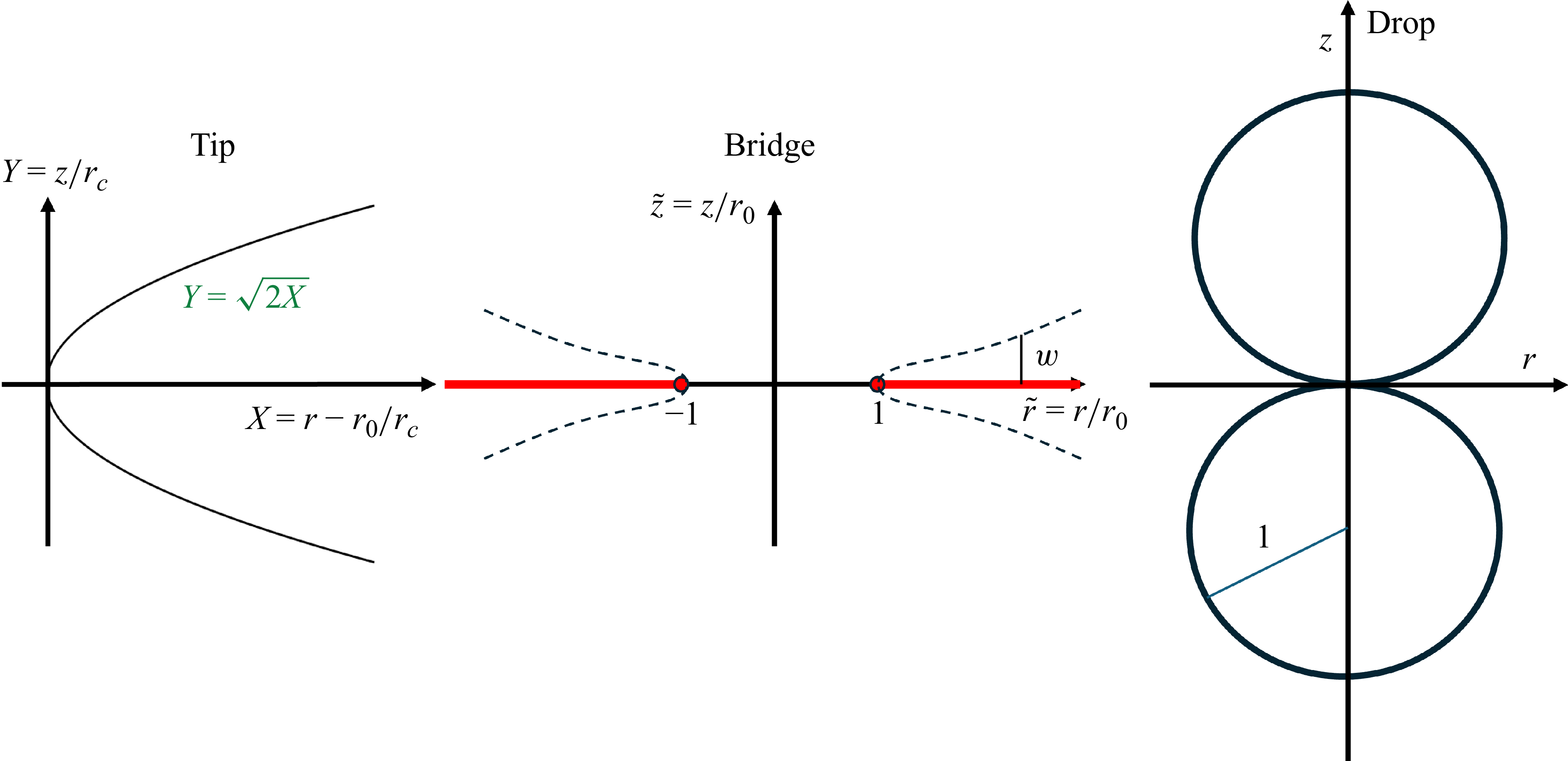
 rc∼r03
 r0
 w∼r02
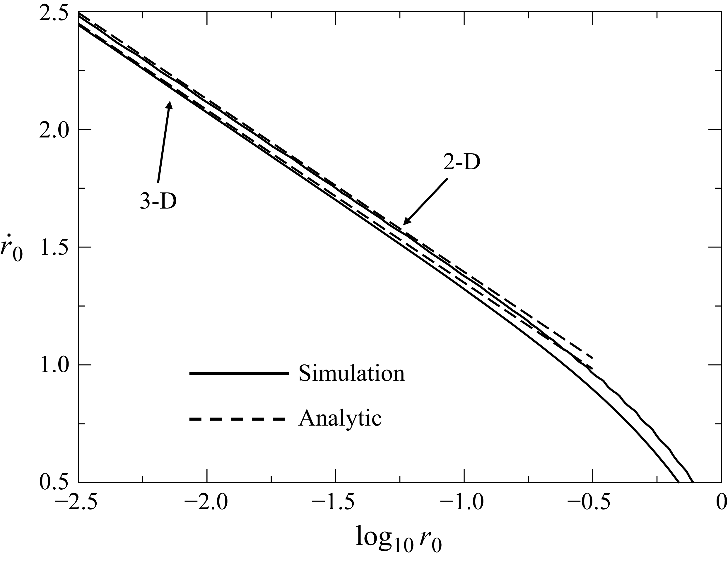
 r0
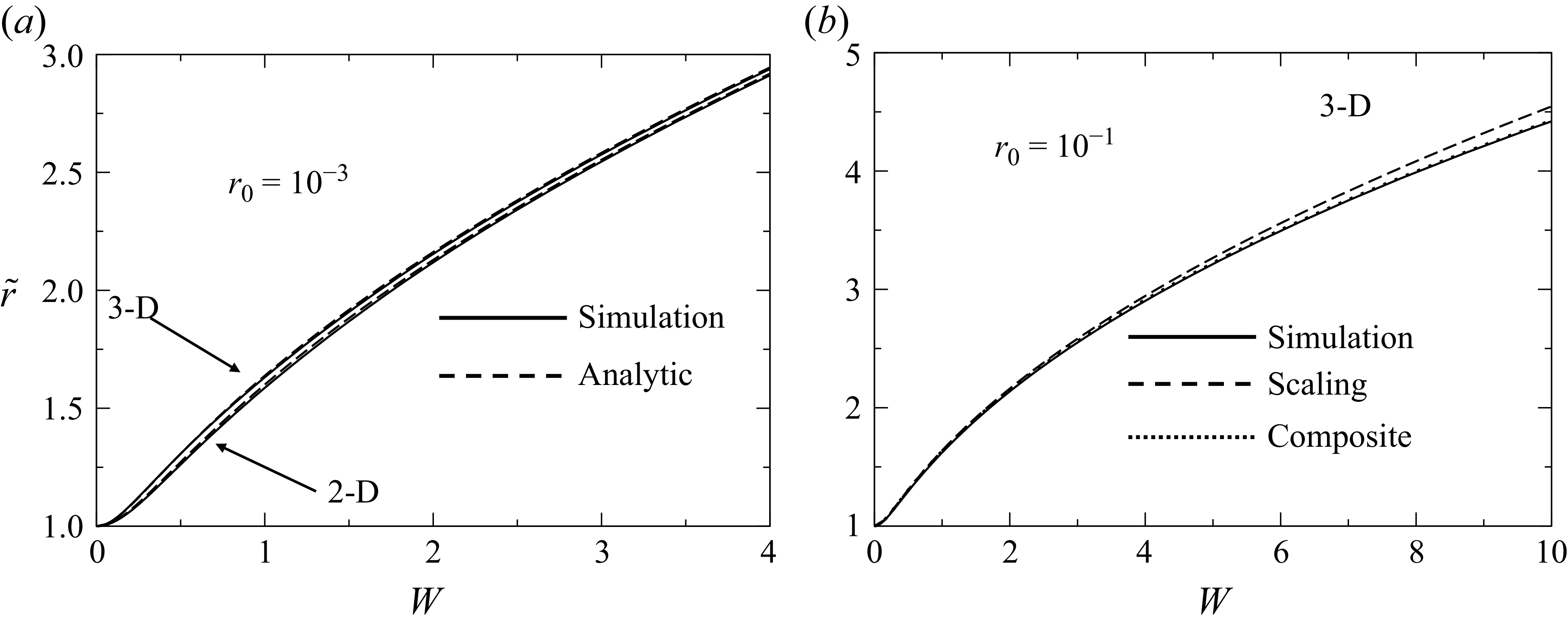
 W(r~)
 W(r~)
 r0≈10−3
 r0=10−1
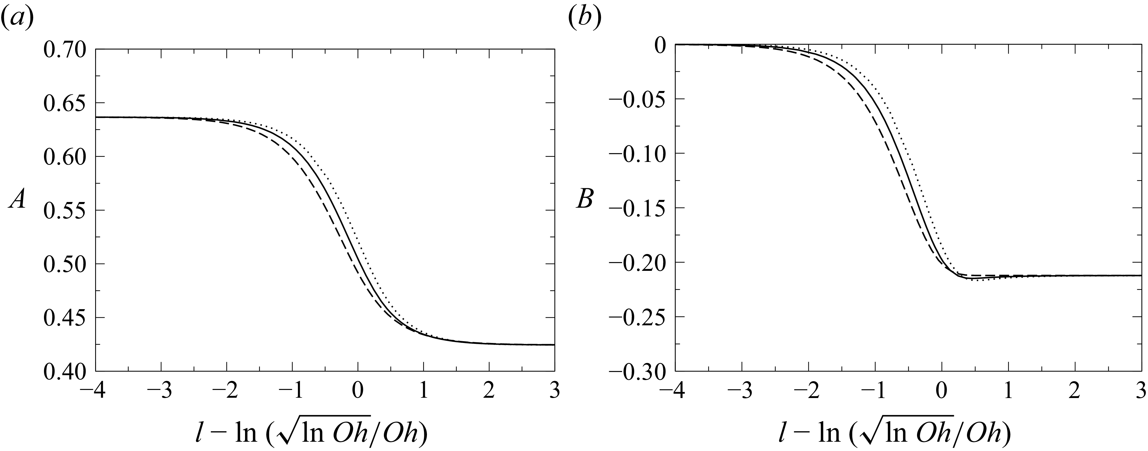
 A
 B
 l=lnr0
 σ
 Oh=10
 Oh=100

 r˙0
 zs/r02
 log10r0
 Oh=100
 Oh=10
 r˙0
 A

 w=r02W(r~)
 Oh=100
 r0=0.0123
 A¯=−0.062
 Oh=10
 r0=0.1
 A¯

 Oh=370
 Oh=0.62
 r0
 Oh=∞
 Oh=1
 A¯=−2/(3π)
 A¯=0
 A¯=−2/(3π)

 E4ψ=0
 2l+1
 l⩾0
 r
 z
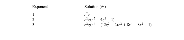
 2l+1
 l≥1
 λ=l


 r0
 r0=10−4
 r0=10−3
 r0=10−4

 Open access

