2 Base flow

We are interested in perturbations developing in the core of a moving vortex structure which constitutes our base flow. We assume that there exist a (moving) local frame where the base flow is locally and, to first approximation, a stationary straight axisymmetric vortex with axial flow. This hypothesis implies that the local curvature radius $\unicode[STIX]{x1D705}$ of the vortex centreline and the shortest distance $\unicode[STIX]{x1D6FF}$ to other vortex structures are both large compared to the core size $a$ of the vortex. In other words, the vortex structure can be described at leading order as a filament. The weak background speed associated with the change of frame is also neglected, which is justified for the applications that we consider in § 8 (Blanco-Rodriguez et al. Reference Blanco-Rodriguez, Le Dizès, Selçuk, Delbende and Rossi2015).

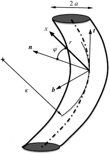
The vortex core dynamics is analysed using a local ‘cylindrical’ coordinate system ( $r,\unicode[STIX]{x1D711},s$ ) constructed from the local Frenet frame ( $\boldsymbol{t},\boldsymbol{n},\boldsymbol{b}$ ) attached to the vortex centreline (see Callegari & Ting Reference Callegari and Ting1978), as described in figure 1.

Figure 1.

Sketch of the local coordinate system in the Frenet frame ( $\boldsymbol{t},\boldsymbol{n},\boldsymbol{b}$ ) of the centreline.

This coordinate system is not orthogonal, but it is related to the orthogonal curvilinear coordinate system ( $r,\unicode[STIX]{x1D703},s$ ) if $\unicode[STIX]{x1D703}=\unicode[STIX]{x1D711}+\int ^{s}\unicode[STIX]{x1D70F}\,\text{d}s$ , $\unicode[STIX]{x1D70F}$ being the torsion. In this frame, the internal vortex structure can be decomposed into multipolar components $f=f_{0}(r)+f_{1}(r)\text{e}^{\text{i}\unicode[STIX]{x1D711}}+f_{2}(r)\text{e}^{2\text{i}\unicode[STIX]{x1D711}}+\cdots$ . Moreover, if we assume that $\unicode[STIX]{x1D705}$ and $\unicode[STIX]{x1D6FF}$ are of the same order, each multipolar component can be expanded in terms of a single parameter $\unicode[STIX]{x1D700}=a/\unicode[STIX]{x1D705}$ .

The leading-order monopolar component is the prescribed underlying straight vortex of velocity–pressure field $\boldsymbol{U}_{m}=(0,V^{(0)}(r),W^{(0)}(r),P^{(0)}(r))$ . Here, we consider the Batchelor vortex profile defined by

(2.1a ) $$\begin{eqnarray}\displaystyle & \displaystyle V^{(0)}=\frac{1-\text{e}^{-r^{2}}}{r}, & \displaystyle\end{eqnarray}$$

(2.1b ) $$\begin{eqnarray}\displaystyle & \displaystyle W^{(0)}=W_{0}\text{e}^{-r^{2}}. & \displaystyle\end{eqnarray}$$

$a$

$\unicode[STIX]{x1D6FA}_{max}^{(0)}=\unicode[STIX]{x1D6E4}/(2\unicode[STIX]{x03C0}a^{2})$

$\unicode[STIX]{x1D6E4}$

$W_{0}$

(2.2) $$\begin{eqnarray}W_{0}=\frac{W_{max}^{(0)}}{\unicode[STIX]{x1D6FA}_{max}^{(0)}a}.\end{eqnarray}$$

Here, we assume that $W_{0}\leqslant 0.5$ such that the vortex remains unaffected by the inviscid swirling-jet instability (Mayer & Powell Reference Mayer and Powell1992).

The dipolar correction is of order $\unicode[STIX]{x1D700}$ and is due to local curvature effects only, as was calculated by Callegari & Ting (Reference Callegari and Ting1978). If the vortex centre is conveniently chosen as a stagnation point of the radial and azimuthal velocity components, a parameter-free expression of this correction is obtained as

(2.3) $$\begin{eqnarray}\boldsymbol{U}_{d}\sim \unicode[STIX]{x1D700}\,\text{Re}(\boldsymbol{U}^{(1)}\text{e}^{\text{i}\unicode[STIX]{x1D711}})=\frac{\unicode[STIX]{x1D700}}{2}\left(\begin{array}{@{}c@{}}\text{i}U^{(1)}(r)\\ V^{(1)}(r)\\ W^{(1)}(r)\\ P^{(1)}(r)\end{array}\right)\text{e}^{\text{i}\unicode[STIX]{x1D711}}+\text{c.c.},\end{eqnarray}$$

where expressions for $U^{(1)}$ , $V^{(1)}$ , $W^{(1)}$ , $P^{(1)}$ are provided in appendix A.

The quadripolar correction responsible for the elliptic instability appears at second order in $\unicode[STIX]{x1D700}$ . As shown in Blanco-Rodriguez et al. (Reference Blanco-Rodriguez, Le Dizès, Selçuk, Delbende and Rossi2015), this correction can be divided into two parts

(2.4) $$\begin{eqnarray}\boldsymbol{U}_{q}\sim \unicode[STIX]{x1D700}^{2}\,\text{Re}((S\boldsymbol{U}^{(2)}+\boldsymbol{U}_{\unicode[STIX]{x1D700}}^{(2)})\text{e}^{2\text{i}\unicode[STIX]{x1D711}})=\frac{\unicode[STIX]{x1D700}^{2}}{2}\left\{S\left(\begin{array}{@{}c@{}}\text{i}U^{(2)}(r)\\ V^{(2)}(r)\\ W^{(2)}(r)\\ P^{(2)}(r)\end{array}\right)+\left(\begin{array}{@{}c@{}}\text{i}U_{\unicode[STIX]{x1D700}}^{(2)}(r)\\ V_{\unicode[STIX]{x1D700}}^{(2)}(r)\\ W_{\unicode[STIX]{x1D700}}^{(2)}(r)\\ P_{\unicode[STIX]{x1D700}}^{(2)}(r)\end{array}\right)\right\}\text{e}^{2\text{i}\unicode[STIX]{x1D711}}+\text{c.c.},\end{eqnarray}$$

where $\boldsymbol{U}^{(2)}$ and $\boldsymbol{U}_{\unicode[STIX]{x1D700}}^{(2)}$ are also provided in appendix A. The second term is a local term generated by curvature. The first term is a strain field contribution: its velocity field reduces to a pure strain field of strain rate $S_{ext}=2\unicode[STIX]{x1D700}^{2}S$ as $r\rightarrow \infty$ . As explained in Blanco-Rodriguez et al. (Reference Blanco-Rodriguez, Le Dizès, Selçuk, Delbende and Rossi2015), the parameter $S$ is the only term which changes from one configuration to another. As we shall see in § 8, it can vanish for helices or vortex ring arrays.

3 Perturbation equations

The dimensionless form of the Euler equations in the orthogonal curvilinear coordinate system $(r,\unicode[STIX]{x1D703},s)$ reads (see Callegari & Ting Reference Callegari and Ting1978)

(3.1a ) $$\begin{eqnarray}\displaystyle & \displaystyle U_{t}+UU_{r}+\frac{V}{r}(U_{\unicode[STIX]{x1D703}}-V)+\frac{WU_{s}}{h}+P_{r}+\frac{\unicode[STIX]{x1D700}}{h}W^{2}\cos \unicode[STIX]{x1D711}=0, & \displaystyle\end{eqnarray}$$

(3.1b ) $$\begin{eqnarray}\displaystyle & \displaystyle V_{t}+UV_{r}+\frac{V}{r}(V_{\unicode[STIX]{x1D703}}+U)+\frac{WV_{s}}{h}+\frac{P_{\unicode[STIX]{x1D703}}}{r}-\frac{\unicode[STIX]{x1D700}}{h}W^{2}\sin \unicode[STIX]{x1D711}=0, & \displaystyle\end{eqnarray}$$

(3.1c ) $$\begin{eqnarray}\displaystyle & \displaystyle W_{t}+UW_{r}+\frac{V}{r}W_{\unicode[STIX]{x1D703}}+\frac{WW_{s}}{h}+\frac{P_{s}}{h}-\frac{\unicode[STIX]{x1D700}}{h}(U\cos \unicode[STIX]{x1D711}-V\sin \unicode[STIX]{x1D711})W=0, & \displaystyle\end{eqnarray}$$

(3.1d ) $$\begin{eqnarray}\displaystyle & \displaystyle \frac{1}{r}(rU)_{r}+\frac{V_{\unicode[STIX]{x1D703}}}{r}+\frac{W_{s}}{h}+\frac{\unicode[STIX]{x1D700}}{h}(U\cos \unicode[STIX]{x1D711}-V\sin \unicode[STIX]{x1D711})=0, & \displaystyle\end{eqnarray}$$

$h=1-\unicode[STIX]{x1D700}r\cos \unicode[STIX]{x1D711}$

$\unicode[STIX]{x1D711}=\unicode[STIX]{x1D703}-\unicode[STIX]{x1D6FC}\unicode[STIX]{x1D700}s$

$\unicode[STIX]{x1D6FC}=\unicode[STIX]{x1D70F}/\unicode[STIX]{x1D705}$

The perturbation equations are obtained by linearizing the Euler equations around the base flow $\boldsymbol{U}\sim \boldsymbol{U}^{(0)}+\text{Re}(\unicode[STIX]{x1D700}\boldsymbol{U}^{(1)}\text{e}^{\text{i}\unicode[STIX]{x1D711}}+\unicode[STIX]{x1D700}^{2}(S\boldsymbol{U}^{(2)}+\boldsymbol{U}_{\unicode[STIX]{x1D700}}^{(2)})\text{e}^{2\text{i}\unicode[STIX]{x1D711}})$ . One should note that we do not consider the monopolar and dipolar corrections to the base flow of the order $\unicode[STIX]{x1D700}^{2}$ as they do not contribute to the elliptic instability. After linearizing, we obtain for the velocity–pressure field $\boldsymbol{u}=(-\text{i}u,v,w,p)$ of the perturbation, a system of the form:

(3.2) $$\begin{eqnarray}\displaystyle (\text{i}\unicode[STIX]{x2202}_{t}\unicode[STIX]{x1D644}+\text{i}\unicode[STIX]{x2202}_{s}\unicode[STIX]{x1D64B}+\unicode[STIX]{x1D648})\boldsymbol{u} & = & \displaystyle \unicode[STIX]{x1D700}(\text{e}^{\text{i}\unicode[STIX]{x1D711}}\unicode[STIX]{x1D649}_{+}^{(1)}+\text{e}^{-\text{i}\unicode[STIX]{x1D711}}\unicode[STIX]{x1D649}_{-}^{(1)})\boldsymbol{u}+\unicode[STIX]{x1D700}^{2}\unicode[STIX]{x1D63F}\boldsymbol{u}\nonumber\\ \displaystyle & & \displaystyle +\,\unicode[STIX]{x1D700}^{2}(\text{e}^{2\text{i}\unicode[STIX]{x1D711}}(S\unicode[STIX]{x1D649}_{+}^{(2)}+\unicode[STIX]{x1D649}_{\unicode[STIX]{x1D700}+}^{(2)})+\text{e}^{-2\text{i}\unicode[STIX]{x1D711}}(S\unicode[STIX]{x1D649}_{-}^{(2)}+\unicode[STIX]{x1D649}_{\unicode[STIX]{x1D700}-}^{(2)}))\boldsymbol{u},\end{eqnarray}$$

where the operators $\unicode[STIX]{x1D644}$ , $\unicode[STIX]{x1D64B}$ , $\unicode[STIX]{x1D648}=\unicode[STIX]{x1D648}(-\text{i}\unicode[STIX]{x2202}_{\unicode[STIX]{x1D711}})$ , $\unicode[STIX]{x1D63F}=\unicode[STIX]{x1D63F}(-\text{i}\unicode[STIX]{x2202}_{s})$ , $\unicode[STIX]{x1D649}_{\pm }^{(1)}=\unicode[STIX]{x1D649}_{\pm }^{(1)}(-\text{i}\unicode[STIX]{x2202}_{\unicode[STIX]{x1D711}},-\text{i}\unicode[STIX]{x2202}_{s})$ , $\unicode[STIX]{x1D649}_{\pm }^{(2)}=\unicode[STIX]{x1D649}_{\pm }^{(2)}(-\text{i}\unicode[STIX]{x2202}_{\unicode[STIX]{x1D711}},-\text{i}\unicode[STIX]{x2202}_{s})$ and $\unicode[STIX]{x1D649}_{\unicode[STIX]{x1D700}\pm }^{(2)}=\unicode[STIX]{x1D649}_{\unicode[STIX]{x1D700}\pm }^{(2)}(-\text{i}\unicode[STIX]{x2202}_{\unicode[STIX]{x1D711}},-\text{i}\unicode[STIX]{x2202}_{s})$ are defined in appendix B.

The left-hand side corresponds to the inviscid perturbation equations of the undeformed Batchelor vortex. The dipolar term (first term) on the right-hand side is responsible for the curvature instability while the quadripolar term (third term) is responsible for the elliptic instability. Note that the perturbation equations for a straight vortex in a strain field (of strain rate $S_{ext}$ ) are obtained from (3.2) by setting $\unicode[STIX]{x1D700}\rightarrow 0$ while keeping $2\unicode[STIX]{x1D700}^{2}S=S_{ext}$ constant.

In this work, we shall also consider weak viscous effects on the perturbations which amount to add a fourth term on the right-hand side of the form

(3.3) $$\begin{eqnarray}\frac{\text{i}}{\mathit{Re}}\unicode[STIX]{x1D651}(-\text{i}\unicode[STIX]{x2202}_{\unicode[STIX]{x1D711}},-\text{i}\unicode[STIX]{x2202}_{s})\boldsymbol{u},\end{eqnarray}$$

where $\unicode[STIX]{x1D651}(-\text{i}\unicode[STIX]{x2202}_{\unicode[STIX]{x1D711}},-\text{i}\unicode[STIX]{x2202}_{s})$ is given by (B 3), and the Reynolds number, $\mathit{Re}$ , by

(3.4) $$\begin{eqnarray}\mathit{Re}=\frac{\unicode[STIX]{x1D6FA}_{max}^{(0)}a^{2}}{\unicode[STIX]{x1D708}}=\frac{\unicode[STIX]{x1D6E4}}{2\unicode[STIX]{x03C0}\unicode[STIX]{x1D708}},\end{eqnarray}$$

with $\unicode[STIX]{x1D708}$ the kinematic viscosity.

4 Growth rate expression for the elliptic instability

As explained by Moore & Saffman (Reference Moore and Saffman1975), the elliptic instability results from the resonant coupling of two Kelvin modes of the undeformed vortex with the quadripolar (elliptic) correction to the vortex. Kelvin modes are normal mode solutions of the left-hand side of (3.2). If they are written as

(4.1) $$\begin{eqnarray}\boldsymbol{u}=\tilde{\boldsymbol{u}}(r)\text{e}^{\text{i}ks+\text{i}m\unicode[STIX]{x1D711}-\text{i}\unicode[STIX]{x1D714}t},\end{eqnarray}$$

$\tilde{\boldsymbol{u}}$ satisfies

(4.2) $$\begin{eqnarray}(\unicode[STIX]{x1D714}\unicode[STIX]{x1D644}-k\unicode[STIX]{x1D64B}+\unicode[STIX]{x1D648}(m))\tilde{\boldsymbol{u}}=0.\end{eqnarray}$$

In the following, we shall assume that each Kelvin mode is normalized such that its pressure amplitude $\tilde{p}$ satisfies

(4.3) $$\begin{eqnarray}\tilde{p}\underset{r\rightarrow 0}{{\sim}}r^{|m|}.\end{eqnarray}$$

Two Kelvin modes of characteristics $(\unicode[STIX]{x1D714}_{A},k_{A},m_{A})$ and $(\unicode[STIX]{x1D714}_{B},k_{B},m_{B})$ are resonantly coupled via the quadripolar correction if they satisfy the condition of resonance (assuming $m_{A}<m_{B}$ )

(4.4a-c ) $$\begin{eqnarray}\unicode[STIX]{x1D714}_{A}=\unicode[STIX]{x1D714}_{B},\quad k_{A}=k_{B},\quad m_{A}=m_{B}-2.\end{eqnarray}$$

The coupling leads to a growth of the Kelvin mode combination with a maximum growth rate scaling as $\unicode[STIX]{x1D700}^{2}$ . Fukumoto (Reference Fukumoto2003) actually explained that for instability there is an additional condition on the energy of the waves which must be opposite or null. For each resonant configuration, a growth rate expression can be obtained from an orthogonality condition using a classical multiple-scale analysis. Details of the method can be found for instance in Eloy & Le Dizès (Reference Eloy and Le Dizès1999). The analysis is more complicated in the presence of curvature because additional terms come from a double interaction with the dipolar field. At order $\unicode[STIX]{x1D700}$ , each Kelvin mode creates contributions of the same frequency and axial wavenumber but azimuthal wavenumber $m\pm 1$ :

(4.5) $$\begin{eqnarray}\boldsymbol{u}_{\pm }^{(1)}=\unicode[STIX]{x1D700}\tilde{\boldsymbol{u}}_{\pm }^{(1)}\text{e}^{\text{i}ks+\text{i}(m\pm 1)\unicode[STIX]{x1D711}-\text{i}\unicode[STIX]{x1D714}t},\end{eqnarray}$$

where

(4.6) $$\begin{eqnarray}(\unicode[STIX]{x1D714}\unicode[STIX]{x1D644}-k\unicode[STIX]{x1D63D}+\unicode[STIX]{x1D648}(m\pm 1))\tilde{\boldsymbol{u}}_{\pm }^{(1)}=\unicode[STIX]{x1D649}_{\pm }^{(1)}(m,k)\tilde{\boldsymbol{u}}.\end{eqnarray}$$

Then, at order $\unicode[STIX]{x1D700}^{2}$ , these contributions generate, by interacting a second time with the dipolar terms, terms of azimuthal wavenumbers $m$ and $m\pm 2$ . These last terms are similar to the terms generated by a single interaction of the initial Kelvin mode with the quadripolar terms. They will, then, provide an additional contribution to the coupling terms. The terms of azimuthal wavenumber $m$ are by contrast expected to modify the frequency of the mode.

The final result can be written as an expression for the complex frequency $\unicode[STIX]{x1D714}$ of the Kelvin mode combination as a function of the axial wavenumber $k$ :

(4.7) $$\begin{eqnarray}\displaystyle & & \displaystyle \left(\unicode[STIX]{x1D714}-\unicode[STIX]{x1D714}_{c}-\text{i}\,\text{Im}\,(\unicode[STIX]{x1D714}_{A})-Q_{A}(k-k_{c})-\text{i}\frac{V_{A}}{\mathit{Re}}-\unicode[STIX]{x1D700}^{2}D_{A}^{(\unicode[STIX]{x1D700})}\right)\nonumber\\ \displaystyle & & \displaystyle \qquad \times \left(\unicode[STIX]{x1D714}-\unicode[STIX]{x1D714}_{c}-\text{i}~\text{Im}\,(\unicode[STIX]{x1D714}_{B})-Q_{B}(k-k_{c})-\text{i}\frac{V_{B}}{\mathit{Re}}-\unicode[STIX]{x1D700}^{2}D_{B}^{(\unicode[STIX]{x1D700})}\right)\nonumber\\ \displaystyle & & \displaystyle \quad =\unicode[STIX]{x1D700}^{4}(SR_{AB}+R_{AB}^{(\unicode[STIX]{x1D700})})(SR_{BA}+R_{BA}^{(\unicode[STIX]{x1D700})}),\end{eqnarray}$$

where it is implicitly assumed that $\unicode[STIX]{x1D714}$ and $k$ are close to the resonant frequency $\unicode[STIX]{x1D714}_{c}$ and wavenumber $k_{c}$ of the 2 modes. The coefficients of this equation are obtained as scalar products with the adjoint Kelvin modes $\tilde{\boldsymbol{u}}_{A}^{\dagger }$ and $\tilde{\boldsymbol{u}}_{B}^{\dagger }$

(4.8a,b ) $$\begin{eqnarray}Q_{A}=\frac{\langle \tilde{\boldsymbol{u}}_{A}^{\dagger },\unicode[STIX]{x1D64B}\,\tilde{\boldsymbol{u}}_{A}\rangle }{\langle \tilde{\boldsymbol{u}}_{A}^{\dagger },\unicode[STIX]{x1D644}\,\tilde{\boldsymbol{u}}_{A}\rangle },\quad Q_{B}=\frac{\langle \tilde{\boldsymbol{u}}_{B}^{\dagger },\unicode[STIX]{x1D64B}\,\tilde{\boldsymbol{u}}_{B}\rangle }{\langle \tilde{\boldsymbol{u}}_{B}^{\dagger },\unicode[STIX]{x1D644}\,\tilde{\boldsymbol{u}}_{B}\rangle },\end{eqnarray}$$

(4.8c,d ) $$\begin{eqnarray}V_{A}=\frac{\langle \tilde{\boldsymbol{u}}_{A}^{\dagger },\unicode[STIX]{x1D651}\,\tilde{\boldsymbol{u}}_{A}\rangle }{\langle \tilde{\boldsymbol{u}}_{A}^{\dagger },\unicode[STIX]{x1D644}\,\tilde{\boldsymbol{u}}_{A}\rangle },\quad V_{B}=\frac{\langle \tilde{\boldsymbol{u}}_{B}^{\dagger },\unicode[STIX]{x1D651}\,\tilde{\boldsymbol{u}}_{B}\rangle }{\langle \tilde{\boldsymbol{u}}_{B}^{\dagger },\unicode[STIX]{x1D644}\,\tilde{\boldsymbol{u}}_{B}\rangle },\end{eqnarray}$$

(4.8e,f ) $$\begin{eqnarray}R_{AB}=\frac{\langle \tilde{\boldsymbol{u}}_{A}^{\dagger },\unicode[STIX]{x1D649}_{+}^{(2)}(m_{B},k_{B})\,\tilde{\boldsymbol{u}}_{B}\rangle }{\langle \tilde{\boldsymbol{u}}_{A}^{\dagger },\unicode[STIX]{x1D644}\,\tilde{\boldsymbol{u}}_{A}\rangle },\quad R_{BA}=\frac{\langle \tilde{\boldsymbol{u}}_{B}^{\dagger },\unicode[STIX]{x1D649}_{-}^{(2)}(m_{A},k_{A})\,\tilde{\boldsymbol{u}}_{A}\rangle }{\langle \tilde{\boldsymbol{u}}_{B}^{\dagger },\unicode[STIX]{x1D644}\,\tilde{\boldsymbol{u}}_{B}\rangle },\end{eqnarray}$$

(4.9a ) $$\begin{eqnarray}\displaystyle D_{A}^{(\unicode[STIX]{x1D700})} & = & \displaystyle \frac{\langle \tilde{\boldsymbol{u}}_{A}^{\dagger },(\unicode[STIX]{x1D63F}(k_{A})\tilde{\boldsymbol{u}}_{A}+\unicode[STIX]{x1D649}_{+}^{(1)}(m_{A}-1,k_{A})\,\tilde{\boldsymbol{u}}_{A-}^{(1)}+\unicode[STIX]{x1D649}_{-}^{(1)}(m_{A}+1,k_{A})\,\tilde{\boldsymbol{u}}_{A+}^{(1)})\rangle }{\langle \tilde{\boldsymbol{u}}_{A}^{\dagger },\unicode[STIX]{x1D644}\,\tilde{\boldsymbol{u}}_{A}\rangle },\end{eqnarray}$$

(4.9b ) $$\begin{eqnarray}\displaystyle D_{B}^{(\unicode[STIX]{x1D700})} & = & \displaystyle \frac{\langle \tilde{\boldsymbol{u}}_{B}^{\dagger },(\unicode[STIX]{x1D63F}(k_{B})\tilde{\boldsymbol{u}}_{B}+\unicode[STIX]{x1D649}_{+}^{(1)}(m_{B}-1,k_{B})\,\tilde{\boldsymbol{u}}_{B-}^{(1)}+\unicode[STIX]{x1D649}_{-}^{(1)}(m_{B}+1,k_{B})\,\tilde{\boldsymbol{u}}_{B+}^{(1)})\rangle }{\langle \tilde{\boldsymbol{u}}_{B}^{\dagger },\unicode[STIX]{x1D644}\,\tilde{\boldsymbol{u}}_{B}\rangle },\end{eqnarray}$$

(4.9c ) $$\begin{eqnarray}\displaystyle R_{AB}^{(\unicode[STIX]{x1D700})} & = & \displaystyle \frac{\langle \tilde{\boldsymbol{u}}_{A}^{\dagger },(\unicode[STIX]{x1D649}_{\unicode[STIX]{x1D700}-}^{(2)}(m_{B},k_{B})\,\tilde{\boldsymbol{u}}_{B}+\unicode[STIX]{x1D649}_{-}^{(1)}(m_{B}-1,k_{B})\,\tilde{\boldsymbol{u}}_{B-}^{(1)})\rangle }{\langle \tilde{\boldsymbol{u}}_{A}^{\dagger },\unicode[STIX]{x1D644}\,\tilde{\boldsymbol{u}}_{A}\rangle },\end{eqnarray}$$

(4.9d ) $$\begin{eqnarray}\displaystyle R_{BA}^{(\unicode[STIX]{x1D700})} & = & \displaystyle \frac{\langle \tilde{\boldsymbol{u}}_{B}^{\dagger },(\unicode[STIX]{x1D649}_{\unicode[STIX]{x1D700}+}^{(2)}(m_{A},k_{A})\,\tilde{\boldsymbol{u}}_{A}+\unicode[STIX]{x1D649}_{+}^{(1)}(m_{A}+1,k_{A})\,\tilde{\boldsymbol{u}}_{A+}^{(1)})\rangle }{\langle \tilde{\boldsymbol{u}}_{B}^{\dagger },\unicode[STIX]{x1D644}\,\tilde{\boldsymbol{u}}_{B}\rangle },\end{eqnarray}$$

(4.10) $$\begin{eqnarray}\langle \boldsymbol{u}_{1},\boldsymbol{u}_{2}\rangle =\int _{0}^{\infty }\boldsymbol{u}_{1}^{\star }\boldsymbol{\cdot }\boldsymbol{u}_{2}r\,\text{d}r=\int _{0}^{\infty }(u_{1}^{\star }u_{2}+v_{1}^{\star }v_{2}+w_{1}^{\star }w_{2}+p_{1}^{\star }p_{2})r\,\text{d}r.\end{eqnarray}$$

The right-hand side of (4.7) represents the coupling terms. Those proportional to $S$ are associated with the strain field while the others correspond to the additional contributions due to the local curvature. The left-hand side of (4.7) gives the dispersion relation of each Kelvin mode close to the resonant point. The terms proportional to $\unicode[STIX]{x1D700}^{2}$ are correction terms induced by curvature. They are not present in a straight vortex configuration. Note also the presence of the terms $\text{i}\text{Im}(\unicode[STIX]{x1D714}_{A})$ and $\text{i}\text{Im}(\unicode[STIX]{x1D714}_{B})$ in the brackets on the left-hand side. These terms have been added to take into account a weak inviscid damping of the modes $A$ and $B$ at the resonant point, associated with the presence of a critical layer singularity (Le Dizès Reference Le Dizès2004). As we shall see below, only one of the two modes exhibits such a damping.

It is worth mentioning that the coefficients $R_{AB}$ , $R_{BA}$ , $R_{AB}^{(\unicode[STIX]{x1D700})}$ and $R_{BA}^{(\unicode[STIX]{x1D700})}$ depend on the normalization of the Kelvin modes. However, equation (4.7) does not, which means that the product on the right-hand side, as well as all the coefficients on the left-hand side, are independent of the Kelvin mode normalization.

The relative amplitude and phase of the resonant Kelvin modes are also provided by the coefficients of (4.7). If the resonant configuration is written as

(4.11) $$\begin{eqnarray}\boldsymbol{u}=a_{A}\tilde{u} _{A}\text{e}^{\text{i}ks+\text{i}m_{A}\unicode[STIX]{x1D711}-\text{i}\unicode[STIX]{x1D714}t}+a_{B}\tilde{u} _{B}\text{e}^{\text{i}ks+\text{i}m_{B}\unicode[STIX]{x1D711}-\text{i}\unicode[STIX]{x1D714}t},\end{eqnarray}$$

where $a_{A}$ and $a_{B}$ are the complex amplitudes of the two Kelvin modes $A$ and $B$ normalized by (4.3), we obtain an amplitude ratio

(4.12) $$\begin{eqnarray}K_{BA}=\frac{a_{B}}{a_{A}}=\frac{\displaystyle \unicode[STIX]{x1D714}-\unicode[STIX]{x1D714}_{c}-\text{i}\,\text{Im}\,(\unicode[STIX]{x1D714}_{A})-Q_{A}(k-k_{c})-\text{i}\frac{V_{A}}{\mathit{Re}}-\unicode[STIX]{x1D700}^{2}D_{A}^{(\unicode[STIX]{x1D700})}}{\unicode[STIX]{x1D700}^{2}(SR_{AB}+R_{AB}^{(\unicode[STIX]{x1D700})})}.\end{eqnarray}$$

5 Resonant Kelvin mode characteristics

The conditions of resonance are not affected by curvature effects at leading order, so the characteristics of the resonant Kelvin modes are the same as for straight configurations. For a Batchelor vortex, these characteristics have already been obtained by Lacaze et al. (Reference Lacaze, Ryan and Le Dizès2007).

For each value of $m$ and $k$ , there exists a discrete number of Kelvin modes, which are identified by a third label $n$ , characterizing their radial complexity (typically, the number of radial oscillation in the vortex core). For a Rankine vortex (with or without axial flow), these modes are neutral with frequencies in the interval $[(m-2)+kW_{0},(m+2)+kW_{0}]$ . For a smooth vortex profile, such as that of the Batchelor vortex, some of the modes become damped owing to the presence of a critical point singularity (point $r_{c}$ where $\unicode[STIX]{x1D714}-m\unicode[STIX]{x1D6FA}^{(0)}(r_{c})-kW^{(0)}(r_{c})=0$ ) in their radial structure (Le Dizès & Lacaze Reference Le Dizès and Lacaze2005; Fabre et al. Reference Fabre, Sipp and Jacquin2006). This damping effect becomes strong when the critical point is within the vortex core. This effect introduces a strong difference in the Kelvin mode spectra of Batchelor and Rankine vortices. Numerous resonances which are possible for the Rankine vortex (Lacaze et al. Reference Lacaze, Birbaud and Le Dizès2005) are not present for the Batchelor vortex, because one of the corresponding modes is now strongly damped (Lacaze et al. Reference Lacaze, Ryan and Le Dizès2007).

Eloy & Le Dizès (Reference Eloy and Le Dizès2001) and Lacaze et al. (Reference Lacaze, Ryan and Le Dizès2007) also observed that the resonant combinations that are the best coupled (that is, providing the largest growth rates) correspond to branches with the same label $n$ . These resonant combinations, termed ‘principal’ modes, have been denoted $(m_{A},m_{B},n)$ where $m_{A}$ and $m_{B}$ are the azimuthal numbers of the two resonant Kelvin modes and $n$ their branch label.

For the Batchelor vortex, Lacaze et al. (Reference Lacaze, Ryan and Le Dizès2007) showed that the principal modes $(-1,1,n)$ progressively disappear as $W_{0}$ increases because a critical point in the structure of the Kelvin mode $B$ ( $m_{B}=1$ ) appears and moves toward the vortex centre. They also showed that other principal modes, which were not present for $W_{0}=0$ , becomes unstable as $W_{0}$ increases.

In an inviscid framework, many resonant configurations were found to give a similar growth rate. As soon as viscosity is present, the complicated structures involving large $m$ , $k$ or $n$ are expected to be strongly damped. For moderate Reynolds numbers (say $\mathit{Re}<10\,000$ ), Lacaze et al. (Reference Lacaze, Ryan and Le Dizès2007) showed that the stability diagram for $W_{0}\leqslant 0.5$ involves only 3 different modes, which are the principal modes $(-1,1,1)$ , $(-2,0,2)$ , $(-2,0,1)$ .

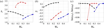
The characteristics of these modes are recalled in figure 2. We have plotted the wavenumber, frequency and critical layer damping of each mode only in the interval where it is expected to exist, that is $0\leqslant W_{0}\leqslant 0.3$ for $(-1,1,1)$ , $0.15\leqslant W_{0}\leqslant 0.35$ for $(-2,0,2)$ and $0.3\leqslant W_{0}\leqslant 0.5$ for $(-2,0,1)$ . On one side of the interval the mode disappears because one of the two resonant waves becomes too strongly damped. It corresponds to the Kelvin mode $B$ ( $m_{B}=1$ ) in $(-1,1,1)$ when $W_{0}>0.3$ and to the Kelvin mode $A$ ( $m_{A}=-2$ ) in $(-2,0,2)$ and $(-2,0,1)$ when $W_{0}<0.15$ and $W_{0}<0.3$ , respectively.

Figure 2.

Characteristics of the principal modes $(-1,1,1)$ (black squares), $(-2,0,2)$ (red triangles), $(-2,0,1)$ (blue circles) as a function of $W_{0}$ . (a) Axial wavenumber $k_{c}$ ; (b) frequency (real part) $\unicode[STIX]{x1D714}_{c}$ ; (c) critical layer damping $\text{Im}(\unicode[STIX]{x1D714}_{A})$ (or $\text{Im}(\unicode[STIX]{x1D714}_{B})$ ) of the resonant Kelvin mode (mode  $B$ with $m_{B}=1$ for $(-1,1,1)$ and mode  $A$ with $m_{A}=-2$ for $(-2,0,2)$ and $(-2,0,1)$ ). The solid lines correspond to the fits provided in appendix C.

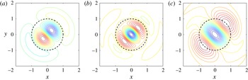
In figure 3, we have displayed the typical spatial structure of the three principal modes for a given set of parameters. We have plotted the vorticity contour of the most unstable principal mode for a particular phase where both Kelvin modes are visible. For each case, we have provided the axial wavenumber, the frequency and the amplitude ratio $K_{BA}$ , defined in (4.12), of the two Kelvin modes that compose the principal mode. Note that the wavenumber and frequency of the principal modes are slightly different from the resonant values $k_{c}$ and $\unicode[STIX]{x1D714}_{c}$ , which are reported in table 1. This shift depends on the values of $\unicode[STIX]{x1D700}$ , $S$ and $\mathit{Re}$ considered.

Figure 3.

Spatial structure of the most dangerous principal modes for typical values of the parameters (here $S=1$ , $\unicode[STIX]{x1D700}^{2}=0.1$ , and $\mathit{Re}=10\,000$ ). Contours of the axial vorticity of the principal mode in an $(x,y)$ plane defined as $\text{Re}[(\tilde{\unicode[STIX]{x1D701}}_{A}(r)\text{e}^{-\text{i}m_{A}\unicode[STIX]{x1D711}}+K_{BA}\tilde{\unicode[STIX]{x1D701}}_{B}(r)\text{e}^{-\text{i}m_{B}\unicode[STIX]{x1D711}})\text{e}^{-\text{i}\unicode[STIX]{x03C0}/2}]$ where $\tilde{\unicode[STIX]{x1D701}}_{A}$ and $\tilde{\unicode[STIX]{x1D701}}_{B}$ are the axial vorticity amplitude of the Kelvin modes $A$ and  $B$ . (a) Mode $(-1,1,1)$ for $W_{0}=0$ ( $k=2.2408$ , $\unicode[STIX]{x1D714}=0.1607\text{i}$ , $K_{BA}=-0.9994\text{i}$ ). (b) Mode $(-2,0,2)$ for $W_{0}=0.2$ ( $k=3.7742$ , $\unicode[STIX]{x1D714}=-0.3759+0.1288\text{i}$ , $K_{BA}=-0.0258+0.3580\text{i}$ ). (c) Mode $(-2,0,1)$ for $W_{0}=0.4$ ( $k=1.9635$ , $\unicode[STIX]{x1D714}=-0.3302+0.1362\text{i}$ , $K_{BA}=-0.0659+1.1721\text{i}$ ).

Table 1.

Characteristics of the main principal modes.

In figure 3, we can clearly see the azimuthal wavenumbers that compose each principal mode. The branch label parameter is also visible. For both modes $(-1,1,1)$ and $(-2,0,1)$ there is a single radial oscillation corresponding to the branch label $n=1$ , while in mode $(-2,0,2)$ , we observe two oscillations as expected for the branch label $n=2$ . The Kelvin mode $m=-2$ of the principal modes $(-2,0,1)$ and $(-2,0,2)$ possesses a critical point singularity (at $r_{c}\approx 2.49$ and $r_{c}\approx 2.36$ , respectively) which is sufficiently far away to not affect the spatial structure of the principal mode in the vortex core.

6 Coefficients of the growth rate formula

In this section we provide the coefficients of the growth rate formula for the resonant configurations giving rise to the principal modes $(-1,1,1)$ , $(-2,0,2)$ , $(-2,0,1)$ .

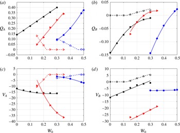
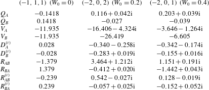
These coefficients are obtained by computing the integrals defined by (4.8) and (4.9) using the same numerical technique as in Lacaze et al. (Reference Lacaze, Ryan and Le Dizès2007). The results are displayed in figures 4 and 5. For each coefficient, we have also plotted an approximate expression, which is provided in appendix C and which corresponds to a simple polynomial fit of the numerical data. These expressions can be used to obtain the elliptic instability growth rate for any values of $W_{0}$ , $\unicode[STIX]{x1D700}$ , $S$ and $\mathit{Re}$ . It is worth mentioning that the linear coefficients $Q_{A}$ , $Q_{B}$ , $V_{A}$ and $V_{B}$ are real when there is no critical layer damping. The coefficients $Q_{A}$ and $V_{A}$ for $(-1,1,1)$ and $Q_{B}$ and $V_{B}$ for $(-2,0,1)$ and $(-2,0,2)$ are therefore always real as they concern the resonant mode with no critical layer ( $m_{A}=-1$ for $(-1,1,1)$ , $m_{B}=0$ for $(-2,0,1)$ and $(-2,0,2)$ ). The imaginary parts of the coefficients $Q_{A}$ and $V_{A}$ (respectively $Q_{B}$ and $V_{B}$ ) become non-zero when $\text{Im}(\unicode[STIX]{x1D714}_{A})$ (respectively $\text{Im}(\unicode[STIX]{x1D714}_{B})$ ) becomes important. The expression $\text{Im}(\unicode[STIX]{x1D714}_{A})+\text{Im}(Q_{A})(k-k_{c})$ represents an approximation to the critical layer damping of the mode $A$ close to $k_{c}$ . It is clear that this expression does not apply when it becomes positive. This has to be kept in mind when using (4.7) away from  $k_{c}$ .

Figure 4.

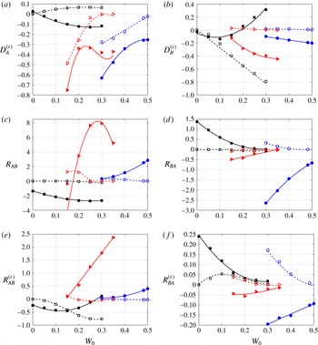
Linear coefficients of the growth rate formula for the principal modes $(-1,1,1)$ (black squares), $(-2,0,2)$ (red triangles), $(-2,0,1)$ (blue circles) as a function of $W_{0}$ . Filled and empty symbols are real part and imaginary part, respectively. The solid and dashed lines are the linear or quadratic fits given in appendix C. (a) $Q_{A}$ , (b) $Q_{B}$ , (c) $V_{A}$ , (d) $V_{B}$ . The coefficients $Q_{B}$ and $V_{B}$ (respectively $Q_{A}$ and $V_{A}$ ) are purely real for the modes $(-2,0,2)$ and $(-2,0,1)$ (respectively for the mode $(-1,1,1)$ ).

Figure 5.

Coupling coefficients of the growth rate formula for the principal modes $(-1,1,1)$ (black squares), $(-2,0,2)$ (red triangles), $(-2,0,1)$ (blue circles) as a function of $W_{0}$ . Filled and empty symbols are real part and imaginary part, respectively. The solid and dashed lines are the polynomial fits given in appendix C. (a)  $D_{A}^{(\unicode[STIX]{x1D700})}$ , (b) $D_{B}^{(\unicode[STIX]{x1D700})}$ , (c) $R_{AB}$ , (d) $R_{BA}$ , (e) $R_{AB}^{(\unicode[STIX]{x1D700})}$ , (f) $R_{BA}^{(\unicode[STIX]{x1D700})}$ .

The coefficients $D_{A}^{(\unicode[STIX]{x1D700})}$ , $D_{B}^{(\unicode[STIX]{x1D700})}$ , $R_{AB}$ , $R_{BA}$ , $R_{AB}^{(\unicode[STIX]{x1D700})}$ and $R_{BA}^{(\unicode[STIX]{x1D700})}$ are coupling coefficients which are generated by interaction with the dipolar and quadripolar corrections to the vortex. The coefficients $R_{AB}$ , $R_{BA}$ are only due to interaction with the strain part of the quadripolar correction. They are the same as those in a straight vortex configuration and were computed in Lacaze et al. (Reference Lacaze, Ryan and Le Dizès2007). The other coupling coefficients are all associated with curvature effects. Note in particular they contain a contribution coming from an interaction with the curvature correction $\boldsymbol{u}_{\pm }^{(1)}$ of each mode (see expressions (4.9a–d )). This function has an intricate structure which may involve one or two critical points. Consequently, the coupling coefficients $D_{A}^{(\unicode[STIX]{x1D700})}$ , $D_{B}^{(\unicode[STIX]{x1D700})}$ , $R_{AB}^{(\unicode[STIX]{x1D700})}$ and $R_{BA}^{(\unicode[STIX]{x1D700})}$ are in general complex even when there is no critical layer damping on the mode itself. Note in particular that the imaginary part of $D_{A}^{(\unicode[STIX]{x1D700})}$ and $D_{B}^{(\unicode[STIX]{x1D700})}$ can be positive, which means that curvature effects on a single Kelvin mode can become destabilizing. This effect is weak but it implies that resonance is a priori not necessary for instability. This surprising result would clearly deserve further studies.

In the following, we shall focus on the three modes $(-1,1,1)$ , $(-2,0,2)$ and $(-2,0,1)$ for the particular values $W_{0}=0$ , $0.2$ and $0.4$ , respectively. The spatial structures of these modes, as well as their frequencies and wavenumbers, have been provided in figure 3 and table 1. The other coefficients of the growth rate equation are given in table 2.

7 Curvature effect

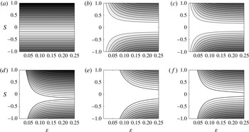
In figure 6, we display the contour levels of the maximum growth rate $\unicode[STIX]{x1D70E}_{max}/\unicode[STIX]{x1D700}^{2}$ for the three modes $(-1,1,1)$ , $(-2,0,2)$ and $(-2,0,1)$ at the values $W_{0}=0$ , 0.2 and 0.4, respectively. Figure 6(a–c) is for an infinite Reynolds number, while (d–f) is for $\mathit{Re}=5000$ . Note the qualitative difference between figure 6(a) and the other panels. The maximum inviscid growth $\unicode[STIX]{x1D70E}_{max}/\unicode[STIX]{x1D700}^{2}$ of the mode $(-1,1,1)$ for $W_{0}=0$ is found not to depend on $\unicode[STIX]{x1D700}$ . For the other modes, $\unicode[STIX]{x1D70E}_{max}/\unicode[STIX]{x1D700}^{2}$ depends on $\unicode[STIX]{x1D700}$ ; this is due to the critical layer damping of the Kelvin mode  $A$ . The inviscid limit is peculiar because the domain of instability covers the entire parameter space. Only the mode $(-1,1,1)$ becomes marginal when $S\approx -0.1735$ . The modes $(-2,0,1)$ and $(-2,0,2)$ are unstable for all values of $S$ but their growth rate is very weak in a large region of the parameter space.

Figure 6.

Contour levels of the maximum instability growth rate $\unicode[STIX]{x1D70E}_{max}/\unicode[STIX]{x1D700}^{2}$ in the $(\unicode[STIX]{x1D700},S)$ plane for $\mathit{Re}=\infty$ (a–c) and $\mathit{Re}=5000$ (d–f). (a,d) Mode $(-1,1,1)$ for $W_{0}=0$ , (b,e) mode $(-2,0,2)$ for $W_{0}=0.2$ , (c,f) mode $(-2,0,1)$ for $W_{0}=0.4$ . Contours are every 0.1. The marginal curve ( $\unicode[STIX]{x1D70E}_{max}=0$ ) is indicated by a thick solid line.

Table 2.

Coefficients of the growth rate equation for the modes $(-1,1,1)$ , $(-2,0,2)$ and $(-2,0,1)$ at the values $W_{0}=0$ , 0.2 and 0.4, respectively.

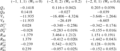
As soon as viscosity is present, a threshold in $\unicode[STIX]{x1D700}$ appears for instability to occur. This threshold increases as $\mathit{Re}$ decreases. For $\mathit{Re}=5000$ , it is already important, as observed in figure 6(d–f). For $\unicode[STIX]{x1D700}=0.25$ , viscosity has stabilized the mode $(-1,1,1)$ in $-0.2<S<-0.15$ , the mode $(-2,0,2)$ in $-0.18<S<0.18$ and the mode $(-2,0,1)$ in $-0.08<S<0.06$ . It should be noted that the viscous damping is stronger on the mode $(-2,0,2)$ (b,e) than on the other modes, as expected from the larger value of the resonant wavenumber of this mode (see table 1).

8 Applications

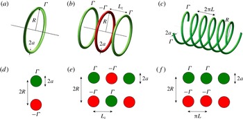
In this section, we apply the results to three different configurations: a single ring, an array of alternate vortex rings and a system of 2 helices as illustrated in figure 7. Each configuration is compared to the equivalent straight configuration, that is a counter-rotating vortex pair, a double array of alternate vortex pairs and a double array of co-rotating vortices, respectively (see figure 7). For both curved and straight configurations, we consider the three different values $W_{0}=0,0.2,0.4$ for which we provide the maximum growth rate of the most unstable modes $(-1,1,1)$ , $(-2,0,2)$ and $(-2,0,1)$ , respectively.

Figure 7.

Sketch of the considered vortex structures. Curved (a–c) and equivalent straight (d–f) configurations. From left to right: a single vortex ring (two counter-rotating vortices), an array of alternate vortex rings (a double array of alternate vortices) and two helices (a double array of co-rotating vortices).

8.1 Vortex ring

For a single ring of radius $R$ and vortex core radius $a$ , the parameter $S$ is given by Blanco-Rodriguez et al. (Reference Blanco-Rodriguez, Le Dizès, Selçuk, Delbende and Rossi2015)

(8.1) $$\begin{eqnarray}S=S^{Ri}=-\frac{3}{16}\left[\log \left(\frac{8}{\unicode[STIX]{x1D700}}\right)-\frac{4}{3}\right],\end{eqnarray}$$

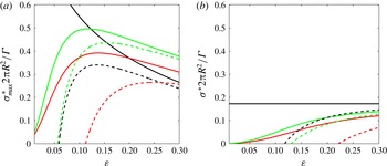
where $\unicode[STIX]{x1D700}=a/R$ . For a given value of the jet parameter $W_{0}$ , the non-dimensionalized elliptic instability growth rate $\unicode[STIX]{x1D70E}_{max}$ is a function of $\unicode[STIX]{x1D700}$ only. In figure 8(a), we have plotted $\unicode[STIX]{x1D70E}_{max}/\unicode[STIX]{x1D700}^{2}$ , that is the dimensional growth rate $\unicode[STIX]{x1D70E}_{max}^{\ast }$ normalized by $\unicode[STIX]{x1D6E4}/(2\unicode[STIX]{x03C0}R^{2})$ for $W_{0}=0$ , 0.2 and 0.4 and two values of the Reynolds number. Figure 8(a) has to be compared with the same plot for 2 straight counter-rotating vortices distant of $2R$ (figure 8 b). We clearly see by comparing these figures that curvature enhances the elliptic instability growth rate. This increase is mainly due to a larger local strain field felt by the vortex ring. In particular, this strain field varies as $\unicode[STIX]{x1D700}^{2}\log (\unicode[STIX]{x1D700})$ for small $\unicode[STIX]{x1D700}$ which explains the divergence of the normalized inviscid growth rate of the mode $(-1,1,1)$ for small $\unicode[STIX]{x1D700}$ in figure 8(a). For the other two modes, the inviscid instability growth rate goes to zero for small $\unicode[STIX]{x1D700}$ due the critical layer damping of the mode  $A$ . In the presence of viscosity, there is an instability threshold in $\unicode[STIX]{x1D700}$ for each mode. The instability threshold is larger for the straight vortices than for the ring.

Figure 8.

Maximum elliptic instability growth rate $\unicode[STIX]{x1D70E}_{max}/\unicode[STIX]{x1D700}^{2}=\unicode[STIX]{x1D70E}_{max}^{\ast }2\unicode[STIX]{x03C0}R^{2}/\unicode[STIX]{x1D6E4}$ versus $\unicode[STIX]{x1D700}=a/R$ for a vortex ring of radius $R$ (a) and 2 counter-rotating vortices distant of $2R$ (b), both of core size  $a$ . Black lines: $W_{0}=0$ (mode $(-1,1,1)$ ), red lines: $W_{0}=0.2$ (mode $(-2,0,2)$ ), green lines: $W_{0}=0.4$ (mode $(-2,0,1)$ ). Solid lines are for $\mathit{Re}=\infty$ , dashed lines for $\mathit{Re}=5000$ . For both cases, the perturbation wavenumber is assumed not to be discretized (see figure 9).

Figure 9.

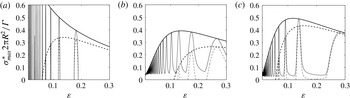
Elliptic instability growth rate $\unicode[STIX]{x1D70E}_{max}/\unicode[STIX]{x1D700}^{2}=\unicode[STIX]{x1D70E}_{max}^{\ast }2\unicode[STIX]{x03C0}R^{2}/\unicode[STIX]{x1D6E4}$ for a vortex ring of radius $R=1/\unicode[STIX]{x1D700}$ for $\mathit{Re}=\infty$ (solid lines) and $\mathit{Re}=5000$ (dashed lines). Thick lines are the maximum growth rate curves plotted in figure 8(a), thin lines are the growth rate curves assuming that the instability wavenumbers are discretized and only take the values $k_{n}=2\unicode[STIX]{x03C0}n\unicode[STIX]{x1D700},n=1,2,3,\ldots$ . (a) $W_{0}=0$ (mode $(-1,1,1)$ ), (b) $W_{0}=0.2$ (mode $(-2,0,2)$ ), (c) $W_{0}=0.4$ (mode $(-2,0,1)$ ).

Figure 8(a) does not take into account that for a ring, the axial wavenumber is discretized and can only take the values $k_{n}=2\unicode[STIX]{x03C0}n/R,n=1,2,3,\ldots$ , that is $k_{n}=2\unicode[STIX]{x03C0}n\unicode[STIX]{x1D700}$ when non-dimensionalized by the core radius. If we take into account this constraint we obtain the growth rate curves shown in figure 9. As can be seen on this figure, the discretization of the wavenumber has a strong influence. Without axial flow, the vortex ring is found to be unstable in short intervals of $\unicode[STIX]{x1D700}$ only. A similar stabilizing effect is observed in the presence of axial flow but if the Reynolds number is sufficiently large, the growth rate remains positive. This is a consequence of the destabilizing effect of the curvature on one of the Kelvin modes when $W_{0}\neq 0$ , which was already noted above. It is worth mentioning that the elliptic instability does not necessarily disappear when the growth rate of the mode that we have considered vanishes. Instead, we expect the growth of other modes associated with different wavenumbers.

For the first mode ( $(-1,1,1)$ at $W_{0}=0$ ), our results can be compared to those obtained by Widnall & Tsai (Reference Widnall and Tsai1977) for a Rankine vortex profile. In the inviscid limit, they obtained with our normalization $\unicode[STIX]{x1D70E}_{max}/\unicode[STIX]{x1D700}^{2}=[(0.214\log (8/\unicode[STIX]{x1D700})-0.228)^{2}-0.028]^{1/2}$ . For the Batchelor vortex with $W_{0}=0$ (that is the Lamb–Oseen vortex), we obtain $\unicode[STIX]{x1D70E}_{max}/\unicode[STIX]{x1D700}^{2}=(0.2585\log (8/\unicode[STIX]{x1D700})-0.5841)$ . The third stabilizing term which is present in the Widnall & Tsai formula corresponds to a detuning effect associated with the coefficients $D_{A}^{(\unicode[STIX]{x1D700})}$ and $D_{B}^{(\unicode[STIX]{x1D700})}$ . This term can be cancelled by slightly modifying the axial wavenumber of the resonant waves, an operation that was not performed by Widnall & Tsai. If we suppress this term, the elliptic instability growth rate of the Lamb–Oseen vortex ring is then found to be smaller than of a Rankine vortex ring as soon as $\unicode[STIX]{x1D700}>0.003$ . This comes from a stronger stabilizing effect of the curvature on the Lamb–Oseen vortex because for straight vortices the opposite result can be proved (Eloy & Le Dizès Reference Eloy and Le Dizès1999).

8.2 Array of alternate vortex rings

We consider an array of alternate vortex rings of radius $R$ and separated by a distance $L_{z}$ (see figure 7). Adapting the results of Blanco-Rodriguez et al. (Reference Blanco-Rodriguez, Le Dizès, Selçuk, Delbende and Rossi2015) obtained for an array of identical rings, we immediately get for an array of ring of alternate signs

(8.2) $$\begin{eqnarray}S=S^{Ri}+S^{DRi},\end{eqnarray}$$

where $S^{Ri}$ is given by (8.1) and

(8.3) $$\begin{eqnarray}S^{DRi}=\frac{1}{4}\mathop{\sum }_{n=1}^{\infty }(-1)^{n}\unicode[STIX]{x1D6EC}_{n}^{3/2}\left(\left(1-\frac{4}{n^{2}\unicode[STIX]{x1D706}^{2}}\right)\boldsymbol{E}(\unicode[STIX]{x1D6EC}_{n})-\boldsymbol{K}(\unicode[STIX]{x1D6EC}_{n})\right),\end{eqnarray}$$

with

(8.4) $$\begin{eqnarray}\unicode[STIX]{x1D6EC}_{n}=\left(1+\frac{n^{2}L_{z}^{2}}{4R^{2}}\right)^{-1},\end{eqnarray}$$

where $\boldsymbol{K}(Z)$ and $\boldsymbol{E}(Z)$ are complete elliptic integrals of the first and second kind, respectively.

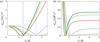
Contrary to vortex rings of the same sign, rings of alternate sign can provide a strain parameter $S$ that can vanish. For $\unicode[STIX]{x1D700}=a/R=0.1$ , $S$ vanishes for $L_{z}/R\approx 1.368$ . In figure 10, we have plotted the maximum inviscid growth rate of the elliptic instability modes documented above for an array of alternate vortex rings and for the equivalent configuration with straight vortices (array of straight counter-rotating vortex pairs of alternate sign). For large $L_{z}/R$ , the growth rate curves converge to the values obtained for a single ring and for a single vortex pair (which is that obtained for $a/R=0.1$ in figure 8). For small $L_{z}/R$ , both configurations provide the same growth rates, that of a single array of straight vortices of alternate sign. Note however that $a/L_{z}$ must remain small for the asymptotic solution to be valid. The results of figure 10 obtained for $a/R=0.1$ are therefore not expected to apply for $L_{z}/R$ smaller than approximately 0.5.

Figure 10.

Maximum elliptic instability growth rate versus $L_{z}/R$ of an array of alternate vortex rings (solid lines) and of an array of straight counter-rotating vortex pairs of alternate sign (dashed lines) for $\unicode[STIX]{x1D700}=a/R=0.1$ and $\mathit{Re}=\infty$ . Black lines: $W_{0}=0$ (mode $(-1,1,1)$ ), red lines: $W_{0}=0.2$ (mode $(-2,0,2)$ ), green lines: $W_{0}=0.4$ (mode $(-2,0,1)$ ). (a) Normalization with $\unicode[STIX]{x1D6E4}/(2\unicode[STIX]{x03C0}L_{z}^{2})$ . (b) Normalization with $\unicode[STIX]{x1D6E4}/(2\unicode[STIX]{x03C0}R^{2})$ . The vertical lines on (a) indicate the value of $L_{z}/R$ where the local strain rate vanishes for each configuration.

Note, finally, that the discretization of the instability wavenumber in an array of rings, which has not been taken into account in figure 10, is similar to that of a single ring. We have assumed that the maximum growth rate was reached for $\unicode[STIX]{x1D700}=0.1$ for the three cases. This is not true. A particular value of $\unicode[STIX]{x1D700}$ exists close to 0.1 where the maximum growth rate is reached but it is actually different for each mode. For the first case (mode $(-1,1,1)$ at $W_{0}=0$ ), this occurs for $\unicode[STIX]{x1D700}=0.12$ , while it is $\unicode[STIX]{x1D700}=0.104$ and $\unicode[STIX]{x1D700}=0.091$ for the second and third cases (mode $(-2,0,2)$ at $W_{0}=0.2$ and mode $(-2,0,1)$ at $W_{0}=0.4$ , respectively).

8.3 Two helical vortices

Blanco-Rodriguez et al. (Reference Blanco-Rodriguez, Le Dizès, Selçuk, Delbende and Rossi2015) have obtained an expression of the strain parameter for $N$ helical Batchelor vortices of radius $R$ and pitch $L$ . For $N=2$ , their expression reduces to

(8.5) $$\begin{eqnarray}\displaystyle S^{MHe} & = & \displaystyle -\frac{3}{16}\log \left(\frac{\unicode[STIX]{x1D6FC}}{(\unicode[STIX]{x1D6FC}^{2}+1)^{3/2}2\unicode[STIX]{x1D700}}\right)-\frac{16(\unicode[STIX]{x1D6FC}^{2}+1)^{3}+\unicode[STIX]{x1D6FC}^{2}(20\unicode[STIX]{x1D6FC}^{4}+12\unicode[STIX]{x1D6FC}^{2}+9)}{96\unicode[STIX]{x1D6FC}^{2}}\nonumber\\ \displaystyle & & \displaystyle +\,\frac{1}{2}\unicode[STIX]{x1D6FC}(\unicode[STIX]{x1D6FC}^{2}+1)^{3/2}+\mathop{\sum }_{m=1}^{\infty }S_{m}(\unicode[STIX]{x1D6FC})\end{eqnarray}$$

with

(8.6a,b ) $$\begin{eqnarray}\unicode[STIX]{x1D6FC}=\frac{L}{R},\quad \unicode[STIX]{x1D700}=\frac{Ra}{R^{2}+L^{2}},\end{eqnarray}$$

and

(8.7) $$\begin{eqnarray}\displaystyle S_{m}(\unicode[STIX]{x1D6FC}) & = & \displaystyle \unicode[STIX]{x1D6FC}(\unicode[STIX]{x1D6FC}^{2}+1)^{3/2}+\frac{3}{16m}-\frac{2(1+\unicode[STIX]{x1D6FC}^{2})^{3}m}{\unicode[STIX]{x1D6FC}^{2}}+\frac{8m^{2}(\unicode[STIX]{x1D6FC}^{2}+1)^{5/2}}{\unicode[STIX]{x1D6FC}^{3}}\nonumber\\ \displaystyle & & \displaystyle \times \,\left(-I_{2m-1}\left(\frac{2m}{\unicode[STIX]{x1D6FC}}\right)+\unicode[STIX]{x1D6FC}I_{2m}\left(\frac{2m}{\unicode[STIX]{x1D6FC}}\right)\right)\left(K_{2m-1}\left(\frac{2m}{\unicode[STIX]{x1D6FC}}\right)+\unicode[STIX]{x1D6FC}K_{2m}\left(\frac{2m}{\unicode[STIX]{x1D6FC}}\right)\right)\nonumber\\ \displaystyle & & \displaystyle +\,4m(\unicode[STIX]{x1D6FC}^{2}+1)^{3/2}I_{2m}\left(\frac{2m}{\unicode[STIX]{x1D6FC}}\right)\left(K_{2m-1}\left(\frac{2m}{\unicode[STIX]{x1D6FC}}\right)+\unicode[STIX]{x1D6FC}K_{2m}\left(\frac{2m}{\unicode[STIX]{x1D6FC}}\right)\right),\end{eqnarray}$$

where $K_{n}(z)$ and $I_{n}(z)$ are modified Bessel functions.

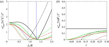
As for alternate rings, the strain rate parameter $S$ can vanish for particular values of $\unicode[STIX]{x1D6FC}$ . This leads to a drop in the elliptic instability growth rate. In figure 11, we have plotted the maximum inviscid growth rate as a function of $L/R$ for $a/R=0.1$ for the three different modes already considered for the ring. The growth rate of the helical vortex configuration is compared to the equivalent ‘straight’ configuration obtained by considering a longitudinal cut of the helical configuration, that is a double array of co-rotating vortices (see figure 7). We observe that for small $L/R$ and for large $L/R$ , both configurations give the same growth rates, which are that of a single array of straight co-rotating vortices and of a straight vortex pair. For intermediate values of $L/R$ , the curves of straight and helical configurations exhibit the same qualitative behaviour: the inviscid growth rate of the mode $(-1,1,1)$ vanishes at a single value of $L/R$ , while the modes $(-2,0,2)$ and $(-2,0,1)$ are stabilized in a finite interval of $L/R$ . However, the numerical values for both configurations are very different. The point of vanishing of the inviscid growth rate of the mode $(-1,1,1)$ occurs at the place where the local strain field felt by the vortex vanishes for the straight configuration. It is slightly shifted to a smaller value for the helical configuration: this is an effect of the additional contribution to the growth rate due to curvature. For $L/R\gtrsim 1$ , the straight configuration is found to be more unstable than the helical one, while it is the opposite for $L/R\lesssim 1$ .

Figure 11.

Maximum elliptic instability growth rate versus $L/R$ of two helical vortices (solid lines) and of an double array of straight co-rotating vortices (dashed lines) for $a/R=0.1$ and $\mathit{Re}=\infty$ . Black lines: $W_{0}=0$ (mode $(-1,1,1)$ ), red lines: $W_{0}=0.2$ (mode $(-2,0,2)$ ), green lines: $W_{0}=0.4$ (mode $(-2,0,1)$ ). (a) Normalization with $\unicode[STIX]{x1D6E4}/(2\unicode[STIX]{x03C0}^{3}L^{2})$ . (b) Normalization with $\unicode[STIX]{x1D6E4}/(2\unicode[STIX]{x03C0}R^{2})$ . The vertical lines on (a) indicate the value of $L/R$ where the local strain rate vanishes for each configuration.

As for the ring arrays, we have to keep in mind that $L/R$ is a priori of $O(1)$ in the asymptotic analysis. Small values of $L/R$ can be considered as long as $a/L$ remains also small. In figure 11, this constraint requires $L/R$ to be much larger than 0.1.