


1. Introduction
Phase-changing liquid films are used for transferring intense heat loads in refrigeration systems (Fernández-Seara & Pardiñas Reference Fernández-Seara and Pardiñas2014) and thermal-management devices such as vapour chambers (Bulut et al. Reference Bulut, Kandlikar and Sozbir2019), grooved heat pipes (Bertossi et al. Reference Bertossi, Lataoui, Ayel, Romestant and Bertin2009) and pulsating heat pipes (Zhang & Nikolayev Reference Zhang and Nikolayev2023). In vapour chambers specifically, heat generated by localised three-dimensional electronic components must be efficiently spread over a larger condenser surface to match the dimensions of the heat sink (Singh & Yesudasan Reference Singh and Yesudasan2025). This multidirectional heat-spreading process is accompanied by capillary-driven liquid transport from the condenser towards the evaporator, leading to non-negligible inertial and extensional effects within the liquid film. Accurately accounting for these effects is crucial for predicting film evolution, interfacial stability and dry-out phenomena. However, the analysis of phase-changing film flows and the development of control strategies to enhance heat transfer are hindered by the high computational cost of the full governing equations (Patankar et al. Reference Patankar, Weibel and Garimella2018) and the limited validity range of existing reduced-order models (Mohamed & Biancofiore Reference Mohamed and Biancofiore2020; Nikolayev Reference Nikolayev2021). To address these limitations. I developed a novel three-dimensional (3-D) integral model that captures the dominant linear and nonlinear dynamics over a broad range of Reynolds numbers while reducing the computational cost by several orders of magnitude.
The dynamics of phase-changing liquid films is commonly described by long-wave models, valid for film aspect ratios
 $\varepsilon \ll 1$
(see reviews by Oron et al. Reference Oron, Davis and Bankoff1997; Craster & Matar Reference Craster and Matar2009; Chattopadhyay et al. Reference Chattopadhyay, Mukhopadhyay and Barua2019). These models are classified by their range of validity in Reynolds number
 ${\textit{Re}}$
(Kalliadasis et al. Reference Kalliadasis, Ruyer-Quil, Scheid and Velarde2011, § 4.9). At low
 ${\textit{Re}}$
, the film dynamics is described by a single Benney–type (BE) equation derived by expanding the dependent variables in powers of
 $\varepsilon$
(Benney Reference Benney1966; Burelbach et al. Reference Burelbach, Bankoff and Davis1988). Using a modified Benney-type equation, Burelbach et al. (Reference Burelbach, Bankoff and Davis1988) studied evaporating films over horizontal plates with particular attention to the dry-out dynamics. For inclined films, Joo et al. (Reference Joo, Davis and Bankoff1991) showed that nonlinear interactions among the Kapitza (H), Marangoni (M) and evaporative (E) modes govern wave breaking, secondary structure formation and dry out, with strong sensitivity to initial conditions. In three dimensions, the mode-coupled H–M and H–E modes generate spanwise-fingering patterns that cannot arise from either mode alone (Joo et al. Reference Joo, Davis and Bankoff1993, Reference Joo, Davis and Bankoff1996).
For larger
 ${\textit{Re}}$
, Mohamed & Biancofiore (Reference Mohamed and Biancofiore2020) showed that the linearised Benney equation overpredicts maximum growth rates and underpredicts cutoff wavenumbers compared with the linearised Navier–Stokes solution, particularly for
 ${{\textit{Re}}} \gtrsim 10$
. Integral-equation models derived via Galerkin projection (Ruyer-Quil & Manneville Reference Ruyer-Quil and Manneville2002) are better suited for moderate
 ${\textit{Re}}$
regimes. Representative examples include the integral boundary-layer model (Aktershev & Alekseenko Reference Aktershev and Alekseenko2013), employing a parabolic trial function, and the weighted-integral boundary-layer (WIBL) model, using polynomial trial and test functions (Craster & Matar Reference Craster and Matar2009; Kalliadasis et al. Reference Kalliadasis, Ruyer-Quil, Scheid and Velarde2011). To reduce discrepancies with the full Navier–Stokes solution, Scheid et al. (Reference Scheid, Kalliadasis, Ruyer-Quil and Colinet2008) developed a simplified second-order WIBL formulation retaining
 $O(\varepsilon ^2)$
viscous corrections while neglecting second-order inertial terms. Although successful in various liquid-film problems (Samanta Reference Samanta2014; Scheid et al. Reference Scheid, Kofman and Rohlfs2016), such models have not yet been used for phase-changing films.
Developing a simplified second-order WIBL model for phase-changing films is crucial for designing control strategies that enhance heat transfer via free-surface waves. For non-evaporating films, experiments (Frisk & Davis Reference Frisk and Davis1972) and simulations (Goren & Mani Reference Goren and Mani1968) show that surface waves can increase heat transfer by up to 80 % relative to flat-film conditions (Miyara Reference Miyara1999). More recent studies (Yoshimura et al. Reference Yoshimura, Nosoko and Nagata1996; Collignon et al. Reference Collignon, Caballina, Lemoine, Markides and Castanet2023) indicate that both periodic and solitary waves substantially enhance heat and mass transfer. In condensing films, Aktershev & Alekseenko (Reference Aktershev and Alekseenko2013) found that specific wave structures increase heat transfer through the combined effects of localised thinning and large recirculation zones.
Achieving such wave states requires control strategies that strongly influence the film dynamics. In practical situations, such as sealed heat pipes (Zhang & Nikolayev Reference Zhang and Nikolayev2021; Pagliarini et al. Reference Pagliarini, Iwata and Bozzoli2023), the free surface is inaccessible, and boundary modifications for mass injection are infeasible. Modulating the substrate temperature thus emerges as the most practical control approach, motivating the development of non-isothermal reduced-order models. Cellier & Ruyer-Quil (Reference Cellier and Ruyer-Quil2020) introduced a novel 2-D second-order thermal model known as the
 $\theta$
model, using thermal relaxation modes as trial functions. This model agrees well with the full energy equation even at large Biot and Péclet numbers (up to
 $O(100)$
). Yet such approaches have not been extended to variable-substrate heating and phase-changing films.
In this work, I develop a model for a liquid film flowing over an incline, in contact with its pure vapour phase, which is assumed to be passive and at saturation pressure and temperature (§ 2). A 3-D simplified second-order WIBL model is coupled to a modified
 $\theta$
model accounting for varying substrate temperatures (§ 3). Assuming weakly evaporating conditions, the interfacial mass flux is taken as a linear function of the free-surface temperature, with the proportionality coefficient derived from the linearised Boltzmann-equation moment method (Aursand & Ytrehus Reference Aursand and Ytrehus2019, § 2.6.4). Sultan et al. (Reference Sultan, Boudaoud and Amar2005) and, more recently, Mohamed & Biancofiore (Reference Mohamed and Biancofiore2024), developed a more general mass-flux closure accounting for both kinetic- and diffusion-driven phase change. The diffusion-limited regime is typically encountered in evaporating films or droplets surrounded by air, where the gas phase becomes nearly saturated with vapour near the free surface. In vapour chambers, however, the intense convective transport in the vapour phase prevents significant accumulation of vapour near the interface. Therefore, gas-phase diffusion does not constitute the dominant resistance to phase change. For this reason, and consistently with common practice in the vapour-chamber literature, a kinetic model was adopted for the mass-flux closure (Patankar et al. Reference Patankar, Weibel and Garimella2018).
The capabilities of the present reduced-order modelling framework for non-isothermal liquid films are summarised in table 1, which compares its features with those of existing models available in the literature.
Comparison of representative long-wave reduced-order models for non-isothermal thin liquid films, highlighting their dimensionality, treatment of the temperature field, inclusion of spatial and temporal substrate-temperature variations (
 $\unicode{x2714}$
), accounting for phase change and long-wave asymptotic order.

Table 1. Long description
A table comparing various models for non-isothermal thin liquid films. The table has 9 rows and 7 columns. The columns are labeled Model, Dim., Var. temp., Substrate temp. var., Phase change, and Order. The rows list different models with their respective attributes. Row 1: Burelbach et al. (1988), Benney, 2-D, no values, no values, Weakly evap., O(ε). Row 2: Joo et al. (1991), Benney, 3-D, no values, no values, Weakly evap., O(ε). Row 3: Scheid et al. (2002), Benney, 2-D, Linear, checkmark, no values, O(ε). Row 4: Ruyer-Quil et al. (2005), WIBL, 2-D, WIBL, no values, no values, O(ε²). Row 5: Scheid et al. (2008), WIBL, 3-D, WIBL, no values, no values, O(ε²). Row 6: Thompson et al. (2019), WIBL, 2-D, Projection, checkmark, no values, O(ε²). Row 7: Cellier & Ruyer-Quil (2020), WIBL, 2-D, θ model, no values, no values, O(ε²). Row 8: This work, WIBL, 3-D, θ model, checkmark, Weakly evap., O(ε²).
The simplified model is validated against the full governing equations. In the linear regime, predictions are compared with linearised 3-D Navier–Stokes equations for both evaporating and condensing films. In the nonlinear regime, film evolution under spatially and temporally varying substrate temperatures is compared with the solution of the Navier–Stokes equation in COMSOL Multiphysics. Finally, the simplified 3-D model is used to investigate the effects of substrate-temperature modulation, showing that it can prevent dry out in evaporating films and modify free-surface wave structures, thereby providing a foundation for control strategies.
2. Problem description
Figure 1 shows the 3-D evaporating/condensing liquid film flowing over a flat plate inclined at an angle
 $\beta$
to the horizontal. The liquid is in contact with its pure vapour phase, which is assumed mechanically and thermodynamically passive and held at the saturation pressure
 $p_s$
and temperature
 $T_s$
(as in Burelbach et al. Reference Burelbach, Bankoff and Davis1988). The liquid has density
 $\rho$
, dynamic viscosity
 $\mu$
, thermal conductivity
 $\lambda$
, thermal diffusivity
 $\kappa$
, surface tension
 $\sigma$
, latent heat
 $L_v$
and thermal capacity at constant pressure
 $C_{\!p}$
, while the vapour density is
 $\rho _v$
.
Schematic representation of a 3-D liquid film flowing under the effect of gravity
 $g$
over a substrate inclined at an angle
 $\beta$
to the horizontal, with an imposed temperature distribution
 $\eta (x,z,t)$
. The phase-changing film is bounded above by its pure vapour phase at saturation pressure
 $p_s$
and temperature
 $T_s$
, with an interfacial mass flux
 $J$
across the free surface.

A Cartesian reference frame
 $\mathcal{O}(x,y,z)$
is defined on the substrate with the
 $x$
-axis streamwise, the
 $y$
-axis normal to the substrate pointing toward the free surface and the
 $z$
-axis spanwise. At the free surface, a local orthonormal reference frame
 $\mathcal{O}(\boldsymbol{n},\boldsymbol{t}_x,\boldsymbol{t}_z)$
is defined, where
 $\boldsymbol{n}$
is the outward unit normal and
 $\boldsymbol{t}_x$
,
 $\boldsymbol{t}_z$
are the tangential unit vectors along the streamwise and spanwise directions, respectively. These vectors are defined as
 \begin{equation} \boldsymbol{n} = \frac {(-\partial _x h, 1, -\partial _z h)^T}{n}, \qquad \boldsymbol{t}_x = \frac {(1, \partial _x h, 0)^T}{t_x}, \qquad \boldsymbol{t}_z = \frac {(0, \partial _z h, 1)^T}{t_z}, \end{equation}
where
 $n$
,
 $t_x$
and
 $t_z$
read
 \begin{equation} n = (1 + (\partial _x h)^2 + (\partial _z h)^2)^{1/2},\quad t_x = (1+(\partial _x h)^2)^{1/2},\quad t_z = (1+(\partial _z h)^2)^{1/2}. \end{equation}
In the remaining, I use the shorthand notation
 $\partial _x h = \partial h/\partial x$
.
The film flows down the inclined plate under the effect of the gravitational acceleration vector
 $\boldsymbol{g}=(g\sin {(\beta)},-g\cos {(\beta)},0)^{T}$
. The solid substrate is held at a prescribed temperature
 $\eta (x,z,t)$
, while the liquid is characterised by its free-surface height
 $h(x,y,t)$
, velocity field
 $\boldsymbol{u}=(u,v,w)^{{T}}$
, pressure
 $p(x,y,z,t)$
and temperature
 $T(x,y,z,t)$
fields with the free-surface temperature
 $T_{\textit{fs}}(x,z,t)$
, streamwise
 $q_x(x,z,t)$
and spanwise
 $q_z(x,z,t)$
flow rates defined as
 \begin{equation} T_{\textit{fs}}(x,z,t)=T|_{y=h},\quad q_x(x,z,t) = \int _{0}^{h}\, u(x,y,z,t)\, {\rm d}y, \quad q_z(x,z,t) = \int _{0}^{h}\, w(x,y,z,t)\, {\rm d}y. \end{equation}
The difference between the liquid temperature at the free surface and the vapour saturation temperature induces both a change in surface tension and a mass flux
 $J(x,z,t)$
due to phase change. Following common practice for thermocapillary flows and previous studies of evaporating films (Palmer Reference Palmer1976), I model these relations as linear functions of
 $T_{\textit{fs}}$
, which read
 \begin{equation} \sigma \bigl (T_{\textit{fs}}\bigr )=\sigma _0-\frac {{\rm d}\sigma }{{\rm d}T}\Big |_{T_s}\bigl (T_{\textit{fs}}-T_s\bigr ), \qquad J=\zeta \bigl (T_{\textit{fs}}-T_s\bigr ), \end{equation}
where
 $\sigma _0$
is the surface tension at the saturation temperature
 $T_s$
, and
 $\zeta$
is the interfacial mass-transfer coefficient. This coefficient is defined as (Aursand & Ytrehus Reference Aursand and Ytrehus2019, § 2.6.4)
 \begin{equation} \zeta = (1.64\,\alpha )\,\rho ^v \, \frac {L_v}{T_s^{3/2}}\, \sqrt {\frac {M_w}{2\pi R_g}}, \end{equation}
where
 $\alpha$
is the accommodation coefficient,
 $M_w$
is the molecular weight of the liquid and
 $R_g$
is the universal gas constant.
The linear mass-flux relation is defined as the linearised Boltzmann-equation moment method (BEMM) model, which accounts for the mass, momentum and energy balance in the Knudsen layer between the free surface and the vapour bulk. This simplified relation is valid in the limit of weak evaporation, corresponding to small driving forces
 $\Delta Z$
. The driving force is the difference between the saturation pressure associated with the free-surface temperature
 $p_s(T_{\textit{fs}})$
of the liquid and the vapour pressure
 $p_s$
. By linearising the saturation line
 $p_s(T)$
,
 $\Delta Z$
is approximated as a function of
 $T_{\textit{fs}}$
, reading
 \begin{equation} \Delta Z = \frac {L_v M_w}{R_g T_s}\,\frac {T_{\textit{fs}}-T_s}{T_s}. \end{equation}
Following the linear assumption (2.4), the linear approximation for the mass flux at the free surface is valid for
 $ \Delta Z\ll 1$
.
2.1. Scaling quantities and non-dimensional groups
The scaling quantities are based on the characteristic viscous scales and the mean film thickness
 $d_0$
at the initial time
 $t=0$
(Williams & Davis Reference Williams and Davis1982; Burelbach et al. Reference Burelbach, Bankoff and Davis1988; Mohamed & Biancofiore Reference Mohamed and Biancofiore2020), which corresponds to the Nusselt flat-film thickness in non-volatile conditions (Kalliadasis et al. Reference Kalliadasis, Ruyer-Quil, Scheid and Velarde2011, § 2.2). The scaling quantities read
 \begin{equation} h_{\textit{ref}} = d_0, \qquad u_{\textit{ref}} = \frac {\nu }{d_0}, \qquad p_{\textit{ref}} = \frac {\rho \nu ^2}{d_0^2},\qquad J_{\textit{ref}} = \frac {\lambda \Delta T_{\textit{ref}}}{d_0 L_v},\qquad t_{\textit{ref}} = \frac {d_0^2}{\nu }, \end{equation}
where
 $\Delta T_{\textit{ref}}$
is the reference temperature difference.
Based on these scaling quantities, the dependent and independent variables are scaled accordingly as follows:
 \begin{equation} (x,y,z)\rightarrow (\hat {x},\hat {y},\hat {z})\,h_{\textit{ref}}, \quad t\rightarrow \hat {t}\,t_{\textit{ref}},\quad (u,v,w)\rightarrow (\hat {w},\hat {v},\hat {w})\,u_{\textit{ref}}, \quad p\rightarrow \hat {p}\,p_{\textit{ref}}, \end{equation}
with the substrate-temperature profile
 $\eta$
, the temperature field
 $T$
and the free-surface temperature
 $T_{\textit{fs}}$
scaled as
 \begin{equation} \eta \rightarrow T_s + \hat {\eta }\,\Delta T_{\textit{ref}},\qquad T\rightarrow T_s + \hat {\theta }\,\Delta T_{\textit{ref}},\qquad T_{\textit{fs}}\rightarrow T_s + \hat {\theta }_s\,\Delta T_{\textit{ref}}, \end{equation}
where
 $\hat {\bullet }$
denotes the non-dimensional variables.
For the derivation of the reduced-order models in § 3.1, slow spatial
 $\hat {X}$
and
 $\hat {Z}$
and time
 $\hat {T}$
scales are introduced. In addition, to guarantee the consistency of the continuity equation, the wall-normal velocity
 $v$
is assumed to be a small quantity. The slow scales read:
 \begin{equation} \hat {X} = \varepsilon \,\hat {x}, \qquad \hat {Z} = \varepsilon \,\hat {z}, \qquad \hat {T} = \varepsilon \, \hat {t}, \qquad \hat {v} = \varepsilon \, \hat {V}, \end{equation}
where
 $\varepsilon \ll 1$
is the film aspect ratio parameter.
The non-dimensional groups arising from the scalings (2.8) and (2.9) are classified into three main categories: hydrodynamic, thermal and phase change. The hydrodynamic non-dimensional numbers are the Reynolds (
 ${\textit{Re}}$
) and the inclination number (
 ${\textit{Ct}}$
) and the non-dimensional surface tension number (
 $\varGamma$
) which are defined as
 \begin{equation} {{\textit{Re}}} =\frac {d_0^3\,g\,\sin {\beta }}{\nu ^2}, \qquad {{\textit{Ct}}} = \frac {d_0^3\,g\,\cos {\beta }}{\nu ^2} = {{\textit{Re}}}\cot \beta , \qquad \varGamma = \frac {\sigma _0\,d_0}{3\rho \nu ^2}. \end{equation}
This definition of
 ${\textit{Re}}$
corresponds to three times the Reynolds number based on the Nusselt scaling,
 ${\textit{{Re}}}_N$
(Kalliadasis et al. Reference Kalliadasis, Ruyer-Quil, Scheid and Velarde2011, § 2.2). Furthermore, replacing
 $d_0$
with the capillary length
 $l_v$
in
 $\varGamma$
yields the classical expression of the Kapitza number
 ${\textit{Ka}}$
.
The relevant thermal non-dimensional numbers are the Prandtl (
 ${\textit{Pr}}$
) number, the Marangoni (
 ${Ma}$
) number and the Marangoni–Reynolds (
 ${\textit{{Re}}}_{M}$
) number, which quantifies the ratio of inertial to viscous effects in thermocapillary-driven motion. These non-dimensional numbers are defined as
 \begin{equation} \textit{Pr} = \frac {\nu \rho C_{\!p}}{\lambda },\quad \quad {\textit{Ma}} = \frac {({\rm d}\sigma /{\rm d}T)\,d_0\,\rho \,C_{\!p}\,\Delta T_{\textit{ref}}}{2\mu \lambda },\quad \quad {\textit{{Re}}}_M = \frac {{\textit{Ma}}}{\textit{Pr}} = \frac {\rho U_{tc} d_0}{2 \mu }, \end{equation}
where
 $U_{tc}$
is the characteristic thermocapillary velocity scale reading
 \begin{equation} U_{tc} = \frac {({\rm d}\sigma /{\rm d}T) \Delta T_{\textit{ref}}}{\mu }. \end{equation}
The non-dimensional group associated with the phase change are the evaporation number (
 ${E}$
), accounting for the ratio between characteristic viscous
 $t_{\textit{ref}}$
over evaporative
 $t_E$
time scales, the vapour recoil number (
 ${Vr}$
), quantifying the strength of the vapour recoil effect, and the kinetic energy (
 $\varPi$
) number, accounting for the intensity of the kinetic energy lost at the free surface due to the phase change. These numbers read
 \begin{equation} {{E}} = \frac {t_{\textit{ref}}} {t_E} =\frac {\lambda \Delta T_{\textit{ref}}}{L_v\,\rho \,\nu },\qquad {\textit{Vr}} = \frac {2{{E}}^2\,\rho }{3\rho _v},\qquad \varPi = \frac {{{E}}^2\,\rho ^2}{2\rho _v^2}\frac {\nu ^2}{d_0^2\,L}. \end{equation}
The non-equilibrium number
 ${K}$
accounts for the thermodynamic equilibrium at the free surface, and is defined as
 \begin{equation} {{K}} = \frac {J_{\textit{ref}}}{\zeta \Delta T_{\textit{ref}}} = \left(\frac {\lambda \,T_s^{3/2}}{r(\alpha )\,d_0\,\rho _{v}\,L^2}\right)\sqrt {\frac {2\pi \,R_g}{M_w}}. \end{equation}
A value of
 ${{K}}=0$
corresponds to the quasi-equilibrium limit, in which the free-surface temperature
 $T_{\textit{fs}}$
is equal to the saturation temperature
 $T_s$
, which in non-dimensional terms corresponds to
 $\hat {\theta }_s=0$
. In the non-volatile limit (
 ${{E}} \rightarrow 0$
), the mass flux at the free surface
 $\hat {J}$
is zero and
 ${K}$
reduces to the inverse of the Biot number, which quantifies the heat transfer from the liquid to the vapour phase.
The reader is referred to table 2 for an overview of the non-dimensional numbers, including their definitions and physical meanings.
Non-dimensional numbers with their definition and physical meaning.

Table 2. Long description
A table with three columns and nine rows. The columns are labeled ‘Nondimensional number’, ‘Definition‘, and ‘Physical meaning‘. The rows list various non-dimensional numbers along with their definitions and physical meanings. Row 1: Reynolds (Re), (d^3 g sin(β)) / v^2, Inertial over viscous stresses. Row 2: Inclination (Ct), (d^3 g sin(β)) / v^2, Measure hydrostatic pressure. Row 3: Surface tension (Γ), (σ d0) / (ρ l v^2), Surface tension over inertia. Row 4: Prandtl (Pr), (ν ρ Cp) / λ, Momentum diffusivity over thermal diffusivity. Row 5: Marangoni (Ma), (γ ΔT d0) / (2 μ κ), Surface tension gradient over inertia. Row 6: Evaporation (E), J_ref / (ρ l ref), Ratio viscous to evaporation time scales. Row 7: Vapour recoil (Vr), E^2 / D, Vapour-recoil force. Row 8: Kinetic energy (Π), E^2 / (D^2 L), Measure kinetic energy flux at the free surface. Row 9: Non-equilibrium (K), J_ref / (ξ ΔT ref), Degree thermodynamic non equilibrium free surface.
2.2. Non-dimensional governing equations
The phase-changing liquid film is described by the non-dimensional mass, momentum and energy conservation equations, which read
 \begin{equation} \boldsymbol{\nabla }\boldsymbol{\cdot }\hat {\boldsymbol{u}} = 0, \end{equation}
 \begin{equation} \partial _t\hat {\boldsymbol{u}} + \hat {\boldsymbol{u}}\boldsymbol{\cdot }\boldsymbol{\nabla }\hat {\boldsymbol{u}} = -\boldsymbol{\nabla }\! \hat {p} +{\nabla} ^2\hat {\boldsymbol{u}} + \hat {\boldsymbol{g}}, \end{equation}
 \begin{equation} \textit{Pr}(\partial _t\hat {\theta } + \hat {\boldsymbol{u}}\boldsymbol{\cdot }\boldsymbol{\nabla }\hat {\theta }) ={\nabla} ^2\hat {\theta }, \end{equation}
where the non-dimensional gravitational acceleration vector
 $\hat {\boldsymbol{g}}$
is given by
 \begin{equation} \hat {\boldsymbol{g}} = ({{\textit{Re}}},-{{\textit{Ct}}},0) ^T. \end{equation}
The kinematic boundary conditions at the substrate (
 $\hat {y}=0$
) read
 \begin{equation} \hat {\boldsymbol{u}} = \boldsymbol{0}, \qquad \hat {\theta } = \hat {\eta }. \end{equation}
At the free surface (
 $\hat {y}=\hat {h}$
), the kinematic boundary condition enforcing the film continuity reads
 \begin{equation} -{{E}} \hat {J}n = \partial _t\hat {h} + \hat {u}\partial _x\hat {h} - v + \hat {w}\,\partial _z\hat {h}, \end{equation}
the thermal boundary, which expresses the heat exchanged with the vapour phase via latent heat and kinetic energy, reads
 \begin{equation} \hat {J} + \varPi \hat {J^3} = - \boldsymbol{\nabla }\hat {\theta }\boldsymbol{\cdot }\boldsymbol{\hat {n}}, \end{equation}
where
 $\hat {J}$
is expressed as a function of
 $\hat {\theta }_s$
via the non-dimensional version of the constitutive relation (2.4), reading
 \begin{equation} \hat {J} = {{K}}^{-1}\,\hat {\theta }_s. \end{equation}
The normal and tangential stress boundary conditions read
 \begin{equation} \frac {3{\textit{Vr}}\hat {J}^2}{2} - \hat {p} + ({\hat {{\unicode{x1D64B}}}}\boldsymbol{\cdot }\boldsymbol{\hat {n}})\boldsymbol{\cdot }\boldsymbol{\hat {n}} = - \left(3\varGamma - \frac {{\textit{Ma}}}{\textit{Pr} }\hat {\theta }_s \right)\boldsymbol{\nabla} _s\boldsymbol{\cdot }\boldsymbol{\hat {n}}, \end{equation}
 \begin{equation} ({\hat {{\unicode{x1D64B}}}}\boldsymbol{\cdot }\boldsymbol{\hat {n}})\boldsymbol{\cdot }\boldsymbol{\hat {t}}_x = \frac {2{\textit{Ma}}}{\textit{Pr} }\partial _x\hat {\theta }_s, \qquad ({\hat {{\unicode{x1D64B}}}}\boldsymbol{\cdot }\boldsymbol{\hat {n}})\boldsymbol{\cdot }\boldsymbol{\hat {t}}_z = \frac {2{\textit{Ma}}}{\textit{Pr} }\partial _z\hat {\theta }_s, \end{equation}
where
 ${\hat {{\unicode{x1D64B}}}}=\boldsymbol{\nabla }\boldsymbol{\hat {u}}+\boldsymbol{\nabla }\boldsymbol{\hat {u}}^T$
is the deviatoric stress tensor and
 $\boldsymbol{\nabla} _s=({\unicode{x1D644}} - \boldsymbol{n}\otimes \boldsymbol{n})\boldsymbol{\cdot }\boldsymbol{\nabla}$
is the surface gradient operator, with
 $\otimes$
representing the dyadic product. For simplicity, the set of governing equations with the corresponding boundary conditions is referred to as the full-model equations in contrast to the reduced-order model equations, which are presented in § 3.1.
By neglecting phase-change effects (
 ${{E}} = {\textit{Vr}} = \varPi = 0$
) and adopting the Nusselt scaling, the above governing equations and boundary conditions reduce to those describing a non-isothermal falling liquid film (Kalliadasis et al. Reference Kalliadasis, Ruyer-Quil, Scheid and Velarde2011, § 2.1).
2.3. Weakly evaporating/condensing flat-state solutions
Considering weak evaporating/condensing conditions (
 ${{E}}\ll 1$
), with a constant and uniform substrate temperature
 $\hat {\eta }$
, the full-model equations admit a slowly varying (
 $\partial _t = O({{E}})$
) and flat (
 $\partial _x \sim 0$
and
 $\partial _z \sim 0$
) film solution. Adapting the derivation described by Burelbach et al. (Reference Burelbach, Bankoff and Davis1988), this solution is given by
 \begin{equation} \overline {H}(\hat {t}) = -K + \sqrt {({{K}}+1)^2-2\,{{E}}\hat {\eta }\hat {t}},\quad \overline {J} = \frac {\hat {\eta }}{\overline {H}(\hat {t})+{{K}}},\quad \overline {U} = {{\textit{Re}}}\overline {H}\,(\hat {t})^2 \left(\bar {y} - \frac {\bar {y}^2}{2}\right)\!, \end{equation}
 \begin{equation} \overline {V} = 0, \qquad \overline {W} = 0, \qquad \overline {P} = {{\textit{Ct}}}\,\overline {H}\,(\hat {t})(1-\bar {y}) + \frac {3}{2}{\textit{Vr}}\bar {J}^2, \qquad \overline {\varTheta } = \hat {\eta }-\overline {J}\,\bar {y}\,\overline {H}, \end{equation}
where
 $\bar {y}=\hat {y}/\hat {h}$
.
In terms of streamwise
 $\overline {Q}_x$
and spanwise
 $\overline {Q}_z$
flow rates and free-surface temperature
 $\overline {\varTheta }_s$
, the solution (2.23) reads
 \begin{equation} \overline {Q}_x = \int _0^{\overline {H}}\,\overline {U}\,{\rm d}\hat {y} = {{\textit{Re}}}\frac {\overline {H}^3}{3}, \quad \overline {Q}_z = \int _0^{\overline {H}}\,\overline {W}\,{\rm d}\hat {y} =0, \quad \overline {\varTheta }_s = \overline {\varTheta }|_{\hat {y}=\overline {H}} = \frac {\hat {\eta }{{K}}}{\overline {H}+{{K}}}. \end{equation}
Depending on the value of
 $\hat {\eta }$
, the film is classified as either evaporating (
 $\hat {\eta }\gt 0$
), when the substrate temperature exceeds the vapour saturation temperature, or condensing (
 $\hat {\eta }\lt 0$
), when the substrate temperature is below the vapour saturation temperature.
In evaporating conditions, the film thins uniformly and disappears at the dry out
 $\hat {t}_d$
given by
 \begin{equation} \hat {t}_d = \frac {1 + 2\,{{K}}}{2{{E}}\hat {\eta }}. \end{equation}
For
 $\hat {\eta }=1$
, the solution recovers the result of Mohamed & Biancofiore (Reference Mohamed and Biancofiore2020) for an evaporating film on an inclined substrate. Furthermore, assuming a horizontal plate (
 ${{\textit{Ct}}} = 0$
), it reduces to the classical solution for an evaporating film originally derived by Burelbach et al. (Reference Burelbach, Bankoff and Davis1988).
When
 ${{E}} = 0$
(the no-evaporation or quasi-equilibrium limit), the solution (2.23) reduces to the classic Nusselt flat-film solution for falling films considered in Kalliadasis et al. (Reference Kalliadasis, Ruyer-Quil, Scheid and Velarde2011, § 2.2) and by Kelly et al. (Reference Kelly, Davis and Goussis1986) for layers with thermocapillarity.
3. Methodology
In this section, I present the Benney-like single-equation model (derived in Joo et al. Reference Joo, Davis and Bankoff1991) and describe the derivation of the WIBL reduced-order model with temperature variations (§ 3.1). I also derive the equations governing the dynamics of small-amplitude waves (§ 4.1) by linearising the WIBL and the full governing equations about the weakly evaporating flat-state solution.
3.1. Derivation reduced-order model
Both the Benney-like and the WIBL reduced-order models rest on the assumptions of weak evaporation
 ${E}$
, strong surface tension
 $\varGamma$
and small variations of kinetic energy
 $\varPi$
at the free surface, reading
 \begin{equation} {{E}} = \varepsilon \,\overline {{{E}}}, \qquad \varGamma = \varepsilon ^{-3}\,\overline {\varGamma }, \qquad \varPi = \varepsilon ^2\,\overline {\varPi }, \end{equation}
where
 $\overline {\bullet }$
denotes
 $O(1)$
quantities and
 $\varepsilon \ll 1$
is the liquid-film parameter, representing the ratio of the characteristic film thickness to the film length. This quantity also accounts for the slow variation of the film in both space and time, as expressed in (2.10).
The starting point for the derivation of the simplified models is the set of second-order boundary-layer equations consistent up to
 $O(\varepsilon ^2)$
(reported in Appendix A). These equations are obtained by rescaling the non-dimensional governing equations and boundary conditions from § 2.2 onto the slow temporal and spatial scales defined in (2.10), applying the assumptions in (3.1) and retaining terms up to
 $O(\varepsilon ^{2})$
.
Based on this set of equations, the integral continuity equation is obtained by integrating the continuity equation (2.16a ) across the film thickness and making use of the kinematic condition at the free surface (2.19), which yields
 \begin{equation} \partial _T \hat {h} + \partial _X \hat {q}_x + \partial _Z \hat {q}_z = -\overline {{{E}}} \hat {J}. \end{equation}
The main difference between the Benney-like and WIBL approaches lies in the representation of the flow rates,
 $\hat {q}_x$
and
 $\hat {q}_z$
and the free-surface temperature
 $\hat {\theta }_s$
. In the Benney-like model, these quantities are enslaved to the film thickness,
 $\hat {h}$
, through an explicit analytical relation, whereas in the WIBL framework,
 $\hat {q}_x$
,
 $\hat {q}_z$
and
 $\hat {\theta }_s$
are free to evolve independent from
 $\hat {h}$
via dedicated integral equations.
3.1.1. Single film-thickness evolution equation
The Benney-like model, derived in two dimensions by Joo et al. (Reference Joo, Davis and Bankoff1991) and then extended to three dimensions by Joo et al. (Reference Joo, Davis and Bankoff1993), neglects terms of order
 $O(\varepsilon)$
or higher in the boundary-layer equation. The starting point of its derivation consists in expanding the dependent variables in
 $\varepsilon$
, reading
 \begin{equation} \hat {u}\approx \hat {u}_0 + \varepsilon \hat {u}_1,\quad \hat {V}\approx \hat {V}_0 + \varepsilon \hat {V}_1,\quad \hat {w}\approx \hat {w}_0 + \varepsilon \hat {w}_1,\quad \hat {p}\approx \hat {p}_0 + \varepsilon \hat {p}_1,\quad \hat {\theta }\approx \hat {\theta }_0. \end{equation}
Injecting (3.3) in the boundary-layer equations, solving the equations at successive orders in
 $\varepsilon$
, computing the flow rate using expressions (2.3) and then substituting the result along with the approximated mass flux
 $\hat {J}$
into (3.2), one obtains the single evolution equation for
 $\hat {h}$
, which in three dimensions reads
 \begin{align} \hat {h}_T &+ \frac {\bar {{{E}}}}{\hat {h}+{{K}}} + {{\textit{Re}}}\hat {h}^2\hat {h}_X + \frac {2{{\textit{Re}}}^2}{15}\partial _X(\hat {h}^6 \hat {h}_X) + \frac {5\bar {{{E}}}{{\textit{Re}}}}{24}\,\partial _X\!\left (\frac {\hat {h}^4}{\hat {h}+{{K}}}\right ) \nonumber \\ &+ \boldsymbol{\nabla }\!\boldsymbol{\cdot }\!\Bigg \{\Bigg [\left (\frac {\hat {h}}{\hat {h}+{{K}}}\right )^2 \left [\frac {{{K}}{\textit{Ma}}}{\textit{Pr} } + {\textit{Vr}}\left (\frac {\hat {h}}{\hat {h}+{{K}}}\right ) \right ] - \frac {{{\textit{Ct}}}}{3}\hat {h}^3 \Bigg ]\boldsymbol{\nabla }\hat {h} \nonumber \\ &+ \bar {\varGamma }\,\hat {h}^3 \boldsymbol{\nabla }({\nabla} ^2\hat {h})\Bigg \} + \bar {{{E}}}\textit{Pr} \left (\frac {\hat {h}}{\hat {h}+{{K}}}\right )^3 \left [ \frac {\bar {{{E}}}}{3(\hat {h}+{{K}})} + \frac {{{\textit{Re}}}}{120}(7\hat {h}-15{{K}})\hat {h}\,\hat {h}_X \right ] = 0. \end{align}
Modelling assumptions and range of validity of the present WIBL-
 $\theta$
model for evaporating and condensing films.

Table 3. Long description
A table summarizing modeling assumptions and their validity ranges for evaporating and condensing films. The table has two columns: Assumption/regime and Validity range and justification. It contains eight rows, each detailing a specific assumption and its corresponding validity range and justification. Row 1: Long-wave approximation, Film aspect ratio epsilon is less than or equal to 1. Breaks down when short-wave modes dominate or strong capillary ridges form. Row 2: Weak-to-moderate inertia, Reynolds number is between 20 and 30. Accuracy decreases for larger Reynolds number where O(epsilon squared) inertial corrections and short-wave instabilities become significant. Row 3: Strong surface tension, Gamma is O(epsilon to the power of negative 3). Surface tension terms appearing at O(1). Alternatively, I consider O(epsilon squared) terms, this assumption can be relaxed to Gamma is O(epsilon to the power of negative 2). Row 4: Linearised phase-change mass flux, Valid for small interfacial temperature jumps delta Z is much less than 1 ((2.6)). Corresponds to linearised kinetic boundary conditions and diffusion-limited vapour transport. Row 5: Moderate evaporation/condensation intensity, Evaporation number E is O(epsilon) or smaller. For large E, interfacial temperature variations induce short-scale dynamics not captured by long-wave theory. Row 6: Variable density and viscosity, Viscosity and density are considered constant. This assumption is valid as long as the temperature variation across the film is not significant and the non-equilibrium number is small K is less than 1. Row 7: Moderate substrate-temperature variation, Variations on scales O(1/epsilon) or slower. Sharp heating fronts generate small-scale structures that the model does not capture. Row 8: No vapour dynamics, Vapour is assumed to be mechanically and thermally passive, maintained at its saturation pressure and temperature. This assumption is valid for sufficiently rapid vapour equilibration and a large vapour thermal capacity relative to that of the liquid film.
Neglecting terms associated with liquid-film phase change (
 $\overline {{{E}}} = {\textit{Vr}} = \overline {\varPi }=0$
) and adopting Nusselt scaling, the above equation reduces to the standard equation for a thermocapillary liquid film (Scheid et al. Reference Scheid, Ruyer-Quil, Thiele, Kabov, Legros and Colinet2005).
3.1.2. Second-order simplified weighted-integral boundary-layer equations
To derive the WIBL model, I assume that the film’s dynamics remains close to the quasi-steady solution introduced in § 2.3, with only small corrections of order
 $O(\varepsilon)$
for the inertial term and
 $O(\varepsilon ^2)$
for the other terms. This assumption implies that the flow preserves coherent wall-normal structure, determined by the viscous–gravity balance in the momentum equations and by the diffusion-dominated behaviour of the energy equation. The assumptions and parameter regimes under which the present WIBL model is valid are summarised in table 3.
Within this framework, the WIBL and
 $\theta$
models are obtained by computing the
 $O(\varepsilon)$
corrections analytically and subsequently applying gauge conditions to derive the evolution equations for
 $\hat {q}_x$
,
 $\hat {q}_z$
and
 $\hat {\theta }_s$
.
The velocity
 $\hat {u}$
,
 $\hat {V}$
and
 $\hat {w}$
and the temperature
 $\hat {\theta }$
are decomposed into the sum of its weakly evaporating steady-state profile
 $\overline {U},\overline {\varTheta }$
, plus terms representing the deviation of the flow rate and temperature distributions from the base state
 $\hat u^{(0)}$
,
 $\hat w^{(0)}$
and
 $\hat {\theta }^{(0)}$
at
 $O(1)$
, and small corrections
 $\hat u^{(1)}$
,
 $\hat w^{(1)}$
and
 $\hat \theta ^{(1)}$
at
 $O(\varepsilon)$
. The resulting approximate expressions for the field quantities are given by
 \begin{equation} \hat {u} \approx \overline {U} + \hat {u}^{(0)} + \hat u^{(1)}, \qquad \hat w \approx \overline U + \hat w^{(0)} + \hat w^{(1)}, \qquad \hat \theta \approx \overline {\varTheta } + \hat \theta ^{(0)} + \hat \theta ^{(1)}. \end{equation}
Although the steady-state solution has only a streamwise velocity component, the spanwise velocity
 $\hat {w}$
is assumed to represent a perturbation of the streamwise base profile, following standard practice in liquid-film reduced-order modelling.
The wall-normal velocity
 $\hat {V}$
is calculated by integrating the continuity equation (A1a
) with only
 $O(1)$
terms and considering the non-penetrability boundary condition at the boundary (A2), which gives
 \begin{equation} \hat {V} = -\int \partial _X(\overline {U} + \hat {u}^{(0)}) + \partial _Z(\overline {U} + \hat {w}^{(0)})\;{\rm d}\hat {y}. \end{equation}
The quantities
 $\hat {u}^{(0)}$
,
 $\hat {w}^{(0)}$
and
 $\hat {\theta }^{(0)}$
are written as the product of a function of
 $\bar {y}$
, which characterises the wall-normal structure of the flow, and amplitude functions
 $a_u^{(0)}(\hat {X},\hat {Z},\hat {T})$
,
 $a_w^{(0)}(\hat {X},\hat {Z},\hat {T})$
and
 $a_\theta ^{(0)}(\hat {X},\hat {Z},\hat {T})$
, corresponding respectively to the streamwise velocity, the spanwise velocity and the free-surface temperature. The components
 $\hat {u}^{(0)}$
,
 $\hat {w}^{(0)}$
and
 $\hat {\theta }^{(0)}$
therefore read
 \begin{equation} \hat u^{(0)} = a_u^{(0)}\!\left (\bar {y} - \frac {\bar {y}^2}{2}\right)\!, \qquad \hat w^{(0)} = a_w^{(0)}\!\left (\bar {y} - \frac {\bar {y}^2}{2}\right )\!, \qquad \hat \theta ^{(0)} = a_\theta ^{(0)}\,v_1(\bar {y}), \end{equation}
where the wall-normal velocity profile structure is equal to the one in the weakly evaporating film solution in (2.23) and
 $v_1(\bar {y})$
represents a linear combination of the first two relaxation thermal eigenmodes with
 $v_1(\bar {y}=1)=1$
. The derivation of this function will be detailed later.
For convenience in the physical interpretation of the results, the values of the amplitude functions are expressed in terms of
 $\hat {h}$
,
 $\hat {q}_x$
,
 $\hat {q}_z$
and
 $\hat {\theta }_s$
. Replacing the decompositions (3.5) up to
 $O(1)$
with (3.7) in the definitions (2.3) gives
 \begin{equation} \int _0^{\hat h} \bigl (\overline U + \hat u^{(0)}\bigr )\,{\rm d}\hat y = \hat q_x, \qquad \int _0^{\hat h} \bigl (\overline U + \hat w^{(0)}\bigr )\,{\rm d}\hat y = \hat q_z, \qquad \overline \varTheta \bigl (\hat h\bigr ) + \hat \theta \bigl (\hat h\bigr )^{(0)} = \hat \theta _s. \end{equation}
Solving (3.8) gives the values of the amplitude functions, reading
 \begin{equation} a_u^{(0)} = \frac {3(\hat q_x - \overline Q_x)}{\hat h}, \qquad a_w^{(0)} = \frac {3(\hat q_z - \overline Q_z)}{\hat h}, \qquad a_\theta ^{(0)} = \hat \theta _s - \overline \varTheta \bigl (\hat h\bigr ). \end{equation}
The wall-normal temperature structure
 $v_1$
is obtained as a linear combination of the two thermal relaxation eigenmodes associated with the eigenvalues with the largest real parts. These modes are determined by solving the linearised temperature equation without convective effects, then approximating their shapes using polynomial functions.
The linearised temperature equation is obtained assuming that the liquid film is in equilibrium under weak evaporation, with a flat-film thickness
 $\overline {H}$
, and considering a small perturbation of the temperature profile,
 $\tilde {\theta } \ll \overline {\varTheta }$
. The solution of the perturbed energy equation (2.16c
) without convective effects is then sought in the form of normal modes in the long-wave limit (i.e.
 $\partial _x \rightarrow 0$
and
 $\partial _{xx} \rightarrow 0$
), which yields
 \begin{equation} \tilde {\theta } = \hat {\tau }(\bar {y})\,exp(\omega \hat {t}), \end{equation}
where
 $\hat {\tau }(\bar {y})$
is the complex amplitude and
 $\omega$
is the complex pulsation.
Injecting (3.10) into the temperature equation for the perturbation temperature and considering the boundary conditions (2.19) and (2.20), gives the following eigenvalue problem with eigenfunction
 $\hat {\tau }(\bar {y})$
and eigenvalue
 $\omega$
, which reads:
 \begin{equation} \textit{Pr} \overline {H}^2\omega \tilde {\tau } = \partial _{yy}\tilde {\tau },\qquad \hat {\tau }|_0 = 0, \qquad (\partial _{y}\hat {\tau })|_{\bar {y}=1} + \tilde {J}\;\overline {H} = 0, \end{equation}
where the wall-normal derivatives are expressed in terms of
 $\bar {y}$
and
 $\tilde {J}$
is assumed proportional to the variation of temperature at the free surface
 $\tilde {J} = \tilde {\theta }|_{\overline {y}=1}{{K}}^{-1}$
.
The solution of the eigenvalue problem (3.11) reads
 \begin{equation} \hat {\tau } = \sin (l\,\bar {y}),\qquad \omega =-\frac {l^2}{\textit{Pr} \overline {H}^2}, \end{equation}
where
 $l$
is a solution of the following equation:
 \begin{equation} \cot {(l)}\,l + \overline {H}/K = 0. \end{equation}
All the eigenvalues
 $\omega$
are negative real numbers corresponding to the relaxation modes from the self-similar temperature profile. Considering asymptotic condition
 $\hat {h}/{{K}}\rightarrow 0$
and
 $\hat {h}/{{K}}\rightarrow \infty$
the solution of (3.13) reads
 \begin{equation} l_n = n\pi \quad \textrm {for} \quad \overline {H}/{{K}}\rightarrow 0,\quad \text{and}\quad l_n = \frac {\pi }{2} + \pi n \quad \textrm {for} \quad \overline {H}/{{K}}\rightarrow \infty , \end{equation}
with
 $n\in \mathbb{N}^+$
.
At large times, only the relaxation eigenmodes with the largest real eigenvalues affect the temperature evolution. Thus only the first two eigenmodes,
 $\hat {\tau }^{(1)}$
and
 $\hat {\tau }^{(2)}$
, associated with
 $n = 1$
and
 $n = 2$
, are considered. For convenience in the construction of the integral model, their values are expressed through approximating functions,
 $\hat {\tau }^{(1)'}$
and
 $\hat {\tau }^{(2)'}$
, respectively, which are based on low-order polynomials with rational fractions. Following the derivation in (Cellier et al. Reference Cellier, Candel and Le2020), the approximated first two eigenfunctions read
 \begin{equation} \hat {\tau }^{(1)'} = \overline {y}(2-\overline {y}) + \frac {\overline {H}}{{{K}}}\overline {y}(1-\overline {y}), \quad \hat {\tau }^{(2)'} = -12\bar {y} \left(\frac {2}{3}-\bar {y}\right) \left(\frac {5}{4}-\bar {y}\right) + 2\frac {\overline {H}}{{{K}}}\bar {y}(1-\bar {y}) \left(\bar {y}-\frac {1}{2}\right)\!. \end{equation}
Figure 2 shows a comparison between the first two long-wave eigenfunctions,
 $\nu _{k=0}^1$
(red continuous line) and
 $\nu _{k=0}^2$
(blue continuous line), computed numerically, and their corresponding polynomial approximations,
 $\hat {\nu }_1$
(red dashed line with squares) and
 $\hat {\nu }_2$
(blue dashed line with circles), for
 $\overline {H}/{{K}}$
equal to (a)
 $10^{-3}$
, (b)
 $16$
and (c)
 $10^{5}$
. The eigenfunctions are scaled by their maximum absolute value. As shown, the polynomial approximations reproduce the behaviour of the numerical eigenfunctions with reasonable accuracy, particularly in the regime of large
 $\overline {H}/{{K}}$
.
Long-wave eigenfunctions
 $\nu _{k=0}^1$
(red contentious line) and
 $\nu _{k=0}^2$
(blue contentious line) and their polynomial approximations
 $\hat {\nu }_1$
(red dashed line with squares) and
 $\hat {\nu }_2$
(blue dashed line with circles) for
 $\overline {H}/{{K}}$
equal to (a)
 $10^{-3}$
, (b)
 $16$
and (c)
 $10^{5}$
.

The structure of the temperature profile in the wall-normal direction,
 $v_1(\bar {y})$
, introduced in (3.9), is expressed as a linear combination of the approximated eigenfunctions (3.15). The coefficients of this linear combination are determined by imposing the following boundary conditions:
 \begin{equation} \tilde {\nu }_1\big |_{1} = 1, \qquad \partial _{yy}\tilde {\nu }_1\big |_{1} = 0. \end{equation}
The resulting expression for
 $v_1(\bar {y})$
reads
 \begin{equation} \hat {\nu }_1 = \bar {y} \left[3 - 3\bar {y} + \bar {y}^2 + \frac {\overline {H}}{{{K}}}\big (2 - 3\bar {y} + \bar {y}^2\big )\right]\!. \end{equation}
Now that I have defined the wall-normal structures and the amplitude functions of the first-order terms for the velocity and temperature fields (3.5), I proceed to compute the first-order corrections
 $\hat u^{(1)}, \hat w^{(1)}, \hat \theta ^{(1)}$
and then derive the integral equations.
The values of the correction terms
 $\hat {u}^{(1)}$
,
 $\hat {w}^{(1)}$
and
 $\hat {\theta }^{(1)}$
are obtained by solving the system (B1) together with the boundary conditions (B2) and (B3), which for brevity have been reported in Appendix B.1.
The evolution equations for
 $\hat {q}_x$
,
 $\hat {q}_z$
and
 $\hat {\theta }_s$
, are obtained by imposing the following conditions:
 \begin{equation} \int _{0}^{\hat {h}} \hat {u}^{(1)} \, {\rm d}\hat {y} = 0, \qquad \int _{0}^{\hat {h}} \hat {w}^{(1)} \, {\rm d}\hat {y} = 0, \qquad \hat {\theta }^{(1)}\big |_{\hat {y}=\hat {h}} = 0, \end{equation}
which are consistent with (3.8) and can be viewed as gauge conditions, defining one among an infinite number of possible velocity decompositions (Samanta et al. Reference Samanta, Ruyer-Quil and Goyeau2011). By imposing conditions (3.18), I obtain a set of nonlinear hyperbolic partial differential equations (PDEs), which, for conciseness, are presented below in a compact form

where
 $\hat {J}$
is linked to
 $\hat {\theta }_s$
by the constitutive relation (2.21) and the expressions of the individual terms, along with their physical interpretations, are provided in Appendix B.2.
The final set of equations for the WIBL model, valid up to
 $O(\varepsilon )$
in the inertial terms and up to
 $O(\varepsilon ^2)$
in the remaining terms with substrate-temperature variations in space and time
 $\hat {\eta }(\hat {X},\hat {T})$
, consists of the continuity equation (3.2), together with the evolution equations (3.19), complemented by the constitutive relation (2.21).
The non-volatile limit corresponds to local thermodynamic equilibrium at the liquid–vapour interface, for which the vapour pressure equals the saturation pressure at the free surface (
 $p_v=p_{s}(T_{\textit{fs}})$
) and no net mass flux occurs across the interface (
 $\hat {J}=0$
). Nevertheless, small temperature variations may still exist along the free surface without substantially altering the local equilibrium conditions. These temperature gradients induce variations in surface tension, thereby generating thermocapillary stresses. The more restrictive isothermal limit corresponds to a uniform temperature field in both the liquid and vapour phases, including at the free surface. As a result, neither phase-change effects (
 $\overline {{{E}}}={\textit{Vr}}=\overline {\varPi }=0$
) nor thermocapillary stresses
 $({\textit{Ma}}=0)$
can arise in this case.
For the non-volatile case and under Nusselt (isothermal) scaling, the continuity and flow rate equations reduce to the thermocapillary falling-film formulation of Kalliadasis et al. (Reference Kalliadasis, Ruyer-Quil, Scheid and Velarde2011, Chapter 8), while, assuming
 $\hat {\eta }$
constant, the thermal equation recovers the 2-D
 $\theta$
model derived by Cellier & Ruyer-Quil (Reference Cellier and Ruyer-Quil2020), with
 ${{K}}^{-1}= {Bi}$
.
The derived WIBL model is consist for
 $\varepsilon \rightarrow 0$
, as expanding the variables
 $\hat {q}_x$
,
 $\hat {q}_z$
and
 $\hat {\theta }_s$
in
 $\varepsilon$
and solving at successive orders yields the relations used in the construction of the single-equation models in § 3.1.1.
3.2. Linear dynamics
In this subsection, I present the linearised governing equations used to investigate linear-stability characteristics of the base-state solution introduced in § 2.3.
To derive these equations, the dependent variable of the Navier–Stokes equations and of the WIBL model are decomposed into their base-state components (2.23) and (2.24), and a small perturbation, reading
 \begin{equation} \begin{gathered} \hat {u} = \overline {U}(\hat {y}) + \iota \tilde {u}(x,y,t),\quad \hat {v} = \overline {V}(\hat {y}) + \iota \tilde {v}(x,y,t),\quad \hat {w} = \overline {W}(\hat {y}) +\iota \tilde {w}(x,y,t),\\ \hat {\theta } = \overline {\varTheta }(\hat {y}) + \iota \tilde {\theta }(x,y,t), \quad \hat {p} = \overline {P}(\hat {y}) + \iota \tilde {p}(x,y,t),\quad \hat {J} = \overline {J} + \iota \tilde {J}(x,t), \quad \hat {h} = \overline {H} + \iota \tilde {h}(x,t),\\ \hat {\theta }_s = \overline {\varTheta }_s + \iota \tilde {\theta }_s,\quad \hat {q}_x = \overline {Q}_x + \iota \tilde {q}_x,\quad \hat {q}_z = \overline {Q}_z + \iota \tilde {q}_z \end{gathered} \end{equation}
where
 $\iota \ll 1$
is a small number and
 $\tilde {\bullet }$
represent the perturbation quantities at
 $O(1)$
.
Substituting the decomposition (3.20) into the full-model equations (presented in § 2.2) and into the WIBL equations (3.2), (3.19) and (2.21), and retaining terms up to
 $O(\iota )$
gives the linearised system governing the evolution of perturbation quantities. Following Joo et al. (Reference Joo, Davis and Bankoff1991) and Mohamed & Biancofiore (Reference Mohamed and Biancofiore2020), the term proportional to
 ${E}$
in the free-surface kinematic condition and in the linearised integral continuity equation is omitted, as it represents the ratio between the initial perturbation amplitude and the evolving base-state film thickness, and therefore does not affect the temporal growth or decay of the perturbations.
The linearised full-model equations are further simplified by eliminating the streamwise and spanwise velocity components. For clarity, the complete derivation of these equations is provided in the supplement material which is available at https://doi.org/10.1017/jfm.2026.11912.
The solution of the linearised equations is sought in the form of normal modes, reading
 \begin{equation} \begin{pmatrix}\tilde {v}\\[3pt] \hat {\theta }\\[3pt] \hat {h}\\[3pt] \hat {J}\end{pmatrix} = \text{Re} \begin{pmatrix}\phi (\hat {y})\\[3pt] \hat {\tau }(\hat {y})\\[3pt] \xi \\[3pt] \mathscr{J}\end{pmatrix}\textrm {exp}\big(i(\boldsymbol{k}\boldsymbol{\cdot }(\hat {x},\hat {z})^T-\omega \,\hat {t}\,)\big),\;\begin{pmatrix}\tilde {q}_x\\[3pt] \tilde {q}_z\\[3pt] \tilde {\theta }_s\end{pmatrix} = \text{Re} \begin{pmatrix}q_x^{\prime }\\[3pt] q_z^{\prime }\\[3pt] \theta _s^{\prime }\end{pmatrix}\textrm {exp}\big(i(\boldsymbol{k}\boldsymbol{\cdot }(\hat {x},\hat {z})^T-\omega \,\hat {t}\,)\big), \end{equation}
where
 $\phi (\hat {y})$
,
 $\tau (\hat {y})$
,
 $\xi$
,
 $\mathscr{J}$
,
 $q_x^{\prime }$
,
 $q_z^{\prime }$
and
 $\theta _s^{\prime }$
are the complex amplitudes,
 $\boldsymbol{k} = (k_x,k_z)^T$
is the wavenumber vector, with
 $k_x$
and
 $k_z$
the real streamwise and spanwise components,
 $\omega =\omega _r + i \omega _i$
is the complex pulsation, with
 $\omega _i$
representing the perturbation growth rate. The disturbance propagates in the direction defined by the angle
 $\varphi = \tan ^{-1}(k_z/k_x)$
with respect to the
 $\hat {x}$
-axis with phase velocity
 $c=\omega _r/\lVert \boldsymbol{k} \rVert$
. For convenience in the long-wave solution, the cosine of the angle
 $\varphi$
is expressed by the variable
 $\hat {k}_{x1}$
, which is defined as
 \begin{equation} \hat {k}_{x1} = \cos {(\varphi )} = k_x/\lVert \boldsymbol{k} \rVert . \end{equation}
Substituting (3.21) into the linearised equations yields the dispersion relation linking
 $\boldsymbol{k}$
to
 $\omega$
.
For the reduced-order models, the dispersion relation is given by a nonlinear algebraic equation, which is solved numerically using the Python routine scipy.optimize.root. For the linearised full-model equations, the dispersion relation is provided by the solution of a generalised eigenvalue problem, where the amplitude functions are the eigenfunctions and
 $\omega$
is the eigenvalue. This eigenvalue problem, known as the Orr–Sommerfeld eigenvalue problem, reads
 \begin{equation} (D^2-\lVert \boldsymbol{k} \rVert ^2)^2\phi + i[(\omega - k_x\overline {U})(D^2-\lVert \boldsymbol{k} \rVert ^2)+D^2\overline {U}k_x] \phi = 0, \end{equation}
 \begin{equation} (D^2 - \lVert \boldsymbol{k} \rVert ^2)\tau - \textit{Pr} [\phi D\overline {\varTheta } -i (\omega -k_x\overline {U})\tau ]= 0, \end{equation}
and with boundary conditions at
 $\hat {y}=0$
 \begin{equation} \phi = 0, \qquad \tau = 0, \end{equation}
with boundary conditions at the free-surface (
 $\hat {y}=\hat {h}$
), reading
 \begin{equation} \xi = \frac {\phi |_{\hat {h}}}{i(k_x\overline {U}|_{\overline {H}}-\omega )}, \end{equation}
 \begin{equation} \begin{gathered} \Big [(D^2-3 \lVert \boldsymbol{k} \rVert ^2) + i(\omega -k_x\overline {U}|_{\overline {H}})\Big ]D\phi +\\+ \lVert \boldsymbol{k} \rVert ^2\Big [-3\mathscr{J}\,\overline {J}\,{\textit{Vr}} + \xi \Big (-{{\textit{Ct}}} + \lVert \boldsymbol{k} \rVert ^2\Big (2\frac {{\textit{Ma}}}{\textit{Pr} }\overline {\varTheta }|_{\overline {H}}-3\varGamma \Big )\Big )\Big ] = 0 ,\end{gathered} \end{equation}
 \begin{equation} (D^2 +\lVert \boldsymbol{k} \rVert ^2)\phi + \lVert \boldsymbol{k} \rVert ^2\frac {2{\textit{Ma}}}{\textit{Pr} }(\xi D\varTheta + \tau ) - ik_x(D^2\overline {U})|_{\overline {H}}\,\xi = 0, \end{equation}
 \begin{equation} (3\overline {J}^2\varPi + 1)\mathscr{J} + D\hat {\tau }|_{\overline {H}} + \xi D^2\varTheta |_{\overline {H}} = 0, \end{equation}
 \begin{equation} \mathscr{J} = \frac {\tau |_{\overline {H}}}{{{K}}} + \frac {D\varTheta |_{\overline {H}}}{{{K}}}\xi , \end{equation}
where
 $D(\bullet )=\partial _{y}(\bullet )$
is the wall-normal differential operator.
In the case of streamwise perturbations (
 $k_z=0$
), the above generalised eigenvalue problem reduces to the one used by Mohamed & Biancofiore (Reference Mohamed and Biancofiore2020). Furthermore, neglecting the phase-change terms
 $\mathscr{J}=0$
, the problem reduces to the one for a falling liquid film with thermocapillary effects, which is reduced to the Orr–Sommerfeld problem in Kalliadasis et al. (Reference Kalliadasis, Ruyer-Quil, Scheid and Velarde2011, § 3.2).
Under long-wave conditions,
 $\lVert \boldsymbol{k} \rVert \ll 1$
, the Orr–Sommerfeld (OS) eigenvalue problem (3.23), (3.24) and (3.25) was also solved by expanding both the eigenfunctions and the eigenvalue
 $\omega$
in a power series of
 $\lVert \boldsymbol{k} \rVert$
, truncated at second order. The expansion takes the form
 \begin{equation} \phi \approx \phi _0 \lVert \boldsymbol{k} \rVert + i \phi _1 \lVert \boldsymbol{k} \rVert ^2 , \quad \tau \approx \tau _0 + \tau _1 \lVert \boldsymbol{k} \rVert ,\quad \xi \approx \xi _0 + i\xi _1 \lVert \boldsymbol{k} \rVert ^2, \quad \omega \approx \omega _0 \lVert \boldsymbol{k} \rVert + i \omega _1 \lVert \boldsymbol{k} \rVert ^2. \end{equation}
Moreover, a strong surface tension condition is assumed, which corresponds to taking the term associated with the surface tension number
 $\varGamma$
in the normal stress boundary condition (3.25b
) to be of order
 $O(1)$
. This assumption can be expressed as
 \begin{equation} \varGamma = \lVert \boldsymbol{k} \rVert ^{-2} \, \varGamma _1. \end{equation}
The approximate values of the eigenfunctions and eigenvalue are obtained by substituting the expansions (3.26) into the OS eigenvalue problem and solving the resulting equations at successive orders in
 $\lVert \boldsymbol{k} \rVert$
. The growth rate and the phase speed obtained with this asymptotic expansion coincide with the solution of the dispersion relation obtained by (Joo et al. Reference Joo, Davis and Bankoff1991) with the Benny-type equation valid up to
 $O(\varepsilon )$
. The resulting solutions are presented in § 4.1.
Regarding the numerical implementation of the OS problem, the eigenvalue problem (3.23), (3.24) and (3.25) was solved numerically using the Chebyshev–tau spectral method (Chapter VII Lanczos Reference Lanczos1988; Johnson Reference Johnson1996) using the Python routine numpy.linalg.eig. Following McFadden et al. (Reference McFadden, Murray and Boisvert1990), the presence of spurious eigenvalues is mitigated by zeroing the last two rows of the differentiation matrices associated with the second derivatives on the right-hand side of the discretised generalised eigenvalue problem. To ensure convergence, a mesh-independence study was performed by comparing the error in the most unstable eigenvalue across different values of
 $N$
, using
 $N=80$
as the reference (see supplementary material). The results indicate that
 $N=20$
provides sufficient accuracy for the most unstable mode while maintaining low computational costs. To further minimise the occurrence of spurious eigenvalues, the solution of the OS problem was repeated with
 $N=20$
and
 $N=50$
, and only those eigenvalues whose relative difference in magnitude, measured using the Euclidean norm
 $\lVert \boldsymbol{\cdot }\rVert$
, remained below
 $0.1$
were retained, following the recommendation of Gardner et al. (Reference Gardner, Trogdon and Douglass1989).
To investigate the growth rate of 3-D waves, I formulated an optimisation problem to identify combinations of non-dimensional parameters and flow conditions that yield the largest growth rate,
 $\omega _i$
, for a perturbation with
 $k_z \neq 0$
. This optimisation was carried out using the non-local algorithm differential evolution, as implemented in the scipy.optimize library. In addition, I explored the
 $({{\textit{Re}}}, \beta )$
parameter space while keeping the remaining non-dimensional groups fixed to determine the boundary separating cases in which the most unstable mode is purely streamwise from those in which it is fully three-dimensional. This threshold was obtained by performing a line search in
 ${\textit{Re}}$
for each prescribed value of
 $\beta$
, and repeating the procedure across successive values of
 $\beta$
.
3.3. Set-up of nonlinear simulations
In this subsection, I outline the set-up used for the 2-D and 3-D nonlinear simulations of an evaporating liquid film subject to spatially varying substrate heating. The 2-D evaporating film is simulated by solving the WIBL model via a Fourier pseudo-spectral method (described in Appendix C) and the full governing equations implemented in COMSOL. In contrast, the 3-D simulations are performed exclusively with the WIBL model, as the computational cost of solving the full-model equations is prohibitive with the available resources, as highlighted by Dietze et al. (Reference Dietze, Rohlfs, Nährich, Kneer and Scheid2014) for a 3-D falling film.
In both the 2-D and 3-D cases, I consider a film flowing over a substrate inclined at
 $\beta = 15^{\circ }$
with water as the working fluid, in equilibrium with its vapour at the saturation temperature,
 $T_{\textit{sat}} = 300\,\mathrm{K}$
. The liquid thermophysical properties are evaluated at
 $300\,\mathrm{K}$
and treated as constant in both space and time. Weak evaporation conditions are assumed, corresponding to an evaporation number
 ${{E}} = 0.01$
. The values of these properties, along with the relevant non-dimensional parameters, are summarised in table 4.
Physical properties, reference quantities and non-dimensional groups for the nonlinear simulation in two and three dimensions, considering a water liquid film over a flat plate inclined at
 $\beta =15^{\circ }$
with respect to the horizontal at
 $T=300\,$
K.

Table 4. Long description
The table is divided into three main sections: Physical properties, Reference quantities, and Non-dimensional groups. It contains 12 rows and 4 columns. The first section, Physical properties, includes the following rows: Density (rho) with a value of 995.6 kg/m^3, Vapour density (rho_v) with a value of 0.03 kg/m^3, Surface tension gradient (dgamma/dT) with a value of 0.15 mN/(m*K), Thermal expansion coefficient (alpha) with a value of 0.10, Dynamic viscosity (mu) with a value of 0.85 mPa*s, Surface tension (gamma_0) with a value of 71.97 mN/m, Latent heat of vaporization (L_v) with a value of 2.256 MJ/kg, Thermal conductivity (lambda) with a value of 0.60 W/(m*K), Specific heat capacity (C_p) with a value of 4.18 kJ/(kg*K), Gas constant (R_g) with a value of 8.314 J/(mol*K), Molecular weight (M_g) with a value of 0.018 kg/mol, and Kinematic viscosity (nu) with a value of 0.85 mm^2/s. The second section, Reference quantities, includes the following rows: Reference film thickness (h_ref) with a value of 162.691 micrometers, Reference temperature difference (Delta T_ref) with a value of 31.96 K, Reference length (x_ref) with a value of 2850 micrometers, and Reference time (t_ref) with a value of 31 milliseconds. The third section, Non-dimensional groups, includes the following rows: Eotvos number (E) with a value of 0.01, Capillary number (Ca) with a value of 56, Reynolds number (Re) with a value of 15, Marangoni number (Ma) with a value of 7.75 x 10^-4, Prandtl number (Pr) with a value of 6, Peclet number (Pe) with a value of 2.21, and Jacob number (K) with a value of 0.04.
Different substrate-heating configurations were investigated. In the 2-D simulation, spatio-temporal temperature variations were considered. For the 3-D simulations, five cases were examined: isothermal conditions, constant evaporation, constant condensation, oscillatory temperature and harmonic temperature variation in both space and time. In the space–time variable-heating case, the harmonic function follows an exponential ramp to avoid abrupt transients at startup. Table 5 summarises the substrate-temperature conditions used in each configuration.
Summary of substrate-temperature functions used for the 2-D and 3-D nonlinear simulations.

Table 5. Long description
The table presents substrate-temperature functions used for 2-D and 3-D nonlinear simulations. It is divided into two main dimensions: 2-D and 3-D. For the 2-D dimension, the table shows an equation involving sine function with variables X-hat and T-hat. It also lists conditions for isothermal, constant evaporation, and constant condensation. For the 3-D dimension, the table shows equations involving cosine functions with variables X-hat, Z-hat, and T-hat for oscillating and variable temperature conditions.
For the variable-heating simulations, the amplitude of the substrate-temperature fluctuations is set to 0.3 with zero mean, to achieve intense heating while ensuring the constraint on the free-surface temperature given by (2.6). This constraint determines the validity limit of the linearised mass-flux approximation (2.4) with (2.5). By substituting the definition of the non-dimensional free-surface temperature from (2.9) into (2.6), the condition that must be satisfied by the free-surface temperature becomes
 \begin{equation} \hat {\theta }s \ll \frac {R_g,T_s^2}{L_v,M_w,\Delta T{\mathrm{ref}}} = 0.56, \end{equation}
which remains above the maximum temperature the substrate reaches during the simulation.
For the 2-D simulations, a domain of non-dimensional length
 $L = 60$
is considered, with periodic boundary conditions. The simulation is run for a non-dimensional time
 $T = 100$
, starting from an initially flat liquid film,
 $\hat {h}(\hat {X},0) = 1$
, and an isothermal liquid at the saturation temperature,
 $\hat {\theta }(\hat {X},\hat {y}) = 0$
. The velocity, pressure and flow rate fields are initialised according to the base-state relations given in (2.23) and (2.24).
The solutions obtained from the WIBL model, expressed in terms of the liquid-film thickness
 $\hat {h}_{\textit{WIBL}}$
and the free-surface temperature
 $\hat {\theta }_{s,\textit{WIBL}}$
, are compared against the corresponding full-model solutions, denoted by
 $\hat {h}_{\textit{full}}$
and
 $\hat {\theta }_{s,\textit{full}}$
. The overall percentage errors for the liquid-film thickness,
 $E_{h,{rel}}(\hat {T})$
, and for the free-surface temperature,
 $E_{\theta _s,\textit{rel}}(\hat {T})$
, are defined as
 \begin{equation} E_{h,{rel}}(\hat {T}) = \frac { \sqrt {\int _0^L \!\big \| \hat {h}_{\textit{WIBL}} - \hat {h}_{\textit{full}} \big \|_2 \, \mathrm{d}\hat {X}} }{\sqrt {\int _0^L \!\big \| \hat {h}_{\textit{full}} \big \|_2 \, \mathrm{d}\hat {X}}},\quad E_{\theta _s,\textit{rel}}(\hat {T}) = \frac {\sqrt {\int _0^L \!\big \| \hat {\theta }_{s,\textit{WIBL}} - \hat {\theta }_{s,\textit{full}} \big \|_2 \, \mathrm{d}\hat {X}} }{\sqrt {\int _0^L \!\big \| \hat {\theta }_{s,\textit{full}} \big \|_2 \, \mathrm{d}\hat {X}}}, \end{equation}
where
 $\| \bullet \|_2$
denotes the
 $L_2$
norm of the variable evaluated at the grid points, with the COMSOL solution remapped over the grid used to solve the WIBL model.
For the 3-D simulations, the domain is a square region defined as
 $\varOmega = \{(\hat {X},\hat {Z}) \in \mathbb{R}^2 \, | \, 0 \lt \hat {X} \lt L,\, 0 \lt \hat {Z} \lt L\}$
with
 $L = 60$
, and periodic boundary conditions are applied in both directions. The final simulation time is
 $\hat {T} = 100$
, consistent with the 2-D runs.
To trigger the development of nonlinear waves, the initial condition consists of a small localised perturbation of the film thickness defined as
 \begin{equation} \hat {h}(\hat {X},\hat {Z},0) = 1 + 0.1 \exp \!\left (-\frac {(\hat {X} - L/4)^2 + (\hat {Z} - L/2)^2}{10}\right )\!, \end{equation}
a uniform substrate temperature equal to the vapour saturation temperature (
 $\hat {\eta } = 0$
), and a flow rate defined by the steady-state relation (2.24).
The results obtained with the different substrate-heating profiles are compared in terms of the time evolution of the minimum film thickness at each time step
 $\hat {T}_k$
,
 $\hat {h}_{\textit{min}}$
, and the spatially averaged mass flux at the free surface, which read
 \begin{equation} \hat {h}_{\textit{min}}(\hat {T}_k) = \textit{min}(\hat {h}(\hat {X},\hat {T}_k),\qquad \langle \hat {J} \rangle _{\varOmega }(\hat {T}_k) = \frac {1}{|\varOmega |} \int _{\varOmega } \frac {\hat {\theta }_s(\hat {X},\hat {Z},\hat {T}_k)}{{{K}}} \, \mathrm{d}\hat {X} \, \mathrm{d}\hat {Z}. \end{equation}
Regarding the numerical implementation, the WIBL equations are discretised in space using a Fourier pseudo-spectral method (Dutykh Reference Dutykh2016) on an equispaced grid of 200 nodes for both the 2-D and 3-D cases (see Appendix C for details). Time integration is carried out using the adaptive Runge–Kutta method of order 5(4) available in scipy.integrate library.
The full-model equations are solved in COMSOL Multiphysics using an arbitrary Lagrangian–Eulerian moving-mesh formulation, in which the interface displacement in the
 $y$
-direction satisfies the kinematic boundary condition at the free surface (2.19). A mesh convergence study (reported in the supplementary material) shows that a mesh with 16 574 elements provides sufficient accuracy. To adequately resolve the thermal and momentum boundary layers that develop near both the substrate and the free surface, the mesh contains ten layers of quadrilateral elements with a stretching factor of 1.5. Time integration is performed using the implicit backwards differentiation formula solver with automatic step-size control and a relative tolerance of
 $10^{-4}$
for residual error control.
4. Results
In this section, I present the results for the linear (§ 4.1) and nonlinear (§ 4.2) dynamics of the 3-D evaporating and condensing liquid film, with particular emphasis on comparing the WIBL prediction with that of the full-model equations.
4.1. Linear-stability analysis
This subsection presents a 3-D linear-stability analysis of the weakly evaporating/condensing flat-film solution introduced in § 2.3. The substrate temperature
 $\hat {\eta }$
is assumed uniform and treated as a control parameter, with
 $\hat {\eta }=1$
corresponding to evaporation and
 $\hat {\eta }=-1$
to condensation. Neutral-stability curves, growth rates and phase speeds are analysed as functions of the wavenumber and key non-dimensional parameters. Predictions from the WIBL model are compared with numerical solutions of the OS eigenvalue problem and with long-wave asymptotic results, which provide analytical estimates near the instability threshold and explicit expressions for the critical parameters. The long-wave solution also serves as a benchmark for assessing the accuracy of the WIBL model, as its predicted growth rates and phase speeds are consistent with those of the 2-D Benney equation (Joo et al. Reference Joo, Davis and Bankoff1991).
For the comparison between the WIBL, OS and long-wave (LW) predictions, the following parameters are fixed:
 ${{E}}=0.2$
,
 $\varPi =0$
,
 $\varGamma =1000$
,
 ${\textit{Pr}} =7$
and
 ${{K}}=0.01$
. The inclination angle
 $\beta$
, Reynolds number
 ${\textit{Re}}$
, vapour-recoil number
 ${Vr}$
, Marangoni number
 ${Ma}$
, mean film thickness
 $\overline {H}$
and non-dimensional time
 $\hat {t}$
are specified on a case-by-case basis. Unless otherwise stated, all results are reported using the scaling (2.8). The WIBL predictions are shown by red dashed lines with squares, LW asymptotic results by blue dash-dotted lines with triangles and OS solutions by solid black lines. For reference, the hydrodynamic mode alone is indicated by dashed grey lines.
In what follows, I first analyse the LW asymptotic solution, then compare WIBL and OS predictions for streamwise and spanwise perturbations, and finally identify the transition between streamwise- and spanwise-dominated instabilities in the
 ${\textit{Re}}$
–
 $\beta$
parameter space.
In the LW limit
 $\lVert \boldsymbol{k} \rVert \ll 1$
, the OS eigenvalue problem (3.23)–(3.25) is solved via an asymptotic expansion in
 $\lVert \boldsymbol{k} \rVert$
(3.26). Substituting this expansion into the governing equations and solving at leading order yields
 \begin{equation} \phi _0(\hat {y}) = \hat {y}^2, \qquad \tau _0(\hat {y}) = \frac {2i\hat {\eta }\hat {y}}{\hat {k}_{x1} {{\textit{Re}}}(\overline {H}+{{K}})^2}, \qquad \omega _0 = {{\textit{Re}}}\overline {H}^{\,2}\,\hat {k}_{x1}, \end{equation}
and at solving at first order yields
 \begin{equation} \begin{aligned} \phi _1(\hat {y}) =& \frac {\hat {y}^3\left ((h+{{K}})^3 \left (60\,\varGamma _1+20\, {{\textit{Ct}}}+\overline {H}\,\hat {k}_{x1}^2\,{{\textit{Re}}}^2\hat {y}\,(\hat {y}-5 \overline {H})\right )-60\hat {\eta }^2 {\textit{Vr}}\right )}{60\,\hat {k}_{x1}\,{{\textit{Re}}}(\overline {H}+{{K}})^3}, \end{aligned} \end{equation}
 \begin{equation} \begin{aligned} \tau _1(\hat {y}) =& \frac {\hat {y}}{60\,\hat {k}_{x1}^2\,\textit{Pr} \,{{\textit{Re}}}^2(\overline {H}+{{K}})^5} \Big [ -5\overline {H}^4\,\textit{Pr} \,\big (72\,\varGamma _1 + 24\,{{\textit{Ct}}} - \hat {k}_{x1}^2\,{{\textit{Re}}}^2\,({{K}}^3\,(6\textit{Pr} +8)\\& + 12\,{{K}}\textit{Pr} \,\hat {y}^2 - 3\,\textit{Pr} \,\hat {y}^3)\big ) + \overline {H}^3\,\textit{Pr} \,\big (\!-360\,{{\textit{Ct}}}\,{{K}} + \hat {k}_{x1}^2\,\textit{Pr} \,{{\textit{Re}}}^2\,(20\,{{K}}^4 + 60\,{{K}}^2\,\hat {y}^2\\& - 50\,{{K}}\hat {y}^3 + 3\,\hat {y}^4) -1080\,\varGamma _1\,{{K}}\big ) + \overline {H}^2\,{{K}}\,\textit{Pr} \,\big (\!-360\,{{\textit{Ct}}}\,{{K}} + \hat {k}_{x1}^2\,\textit{Pr} \,{{\textit{Re}}}^2\hat {y}^2\,(20\,{{K}}^2\\& - 60\,{{K}}\hat {y} + 9\,\hat {y}^2) - 1080\,\varGamma _1\,{{K}}\big ) + 3\,\overline {H}\,\big (\!-10\,{{K}}^3\,\textit{Pr} \,(12\,\varGamma _1 + 4\,{{\textit{Ct}}} + \hat {k}_{x1}^2\,\textit{Pr} \,{{\textit{Re}}}^2\,\hat {y}^3)\\& + 3\,{{K}}^2\,\hat {k}_{x1}^2\,\textit{Pr} ^2\,{{\textit{Re}}}^2\,\hat {y}^4 + 80\,{{K}}\,{\textit{Ma}} + 120\,\textit{Pr} \,{\textit{Vr}}\big ) - 8\,\overline {H}^7\,\hat {k}_{x1}^2\,(\textit{Pr} -5)\,\textit{Pr} \,{{\textit{Re}}}^2\\& + 2\,\overline {H}^6\,{{K}}\hat {k}_{x1}^2 \,\textit{Pr} (60-13 \textit{Pr} )\,{{\textit{Re}}}^2 + 4\,\overline {H}^5\,\hat {k}_{x1}^2\,\textit{Pr} \,{{\textit{Re}}}^2\,(5\,\textit{Pr} \,\bar {y}^2 - 2\,{{K}}^2\,(\textit{Pr} -15))\\& + {{K}}^2\,\big ({{K}}\hat {k}_{x1}^2\,\textit{Pr} ^2\,{{\textit{Re}}}^2\,\hat {y}^3\,(3\hat {y} - 5{{K}}) + 240\,{\textit{Ma}}\big ) \Big ], \end{aligned} \end{equation}
 \begin{equation} \omega _1 = -\varGamma _1\,\overline {H}^3 - \frac {{{\textit{Ct}}}}{3}\,\overline {H}^3 + \frac {2}{15}\,\overline {H}^6\,\hat {k}_{x1}^2\, {{\textit{Re}}}^2 +\frac {\hat {\eta }^2 \,\overline {H}^3\,{\textit{Vr}}}{(\overline {H}+{{K}})^3}+\frac {\hat {\eta }\,\overline {H}^2\,{{K}}\,{\textit{Ma}}}{\textit{Pr} \,(\overline {H}+{{K}})^2}. \end{equation}
The eigenvalues
 $\omega = \omega _0\lVert \boldsymbol{k}\rVert + i\omega _1\lVert \boldsymbol{k}\rVert ^2$
coincide with those obtained by solving the algebraic dispersion relation associated with the 3-D Benney equation, as reported in Joo et al. (Reference Joo, Davis and Bankoff1993). In addition, considering the non-dimensional film thickness
 $ \overline {H} = 1$
, evaporating conditions (
 $\hat {\eta } = 1$
) and purely streamwise perturbations (
 $\hat {k}_{x1}=1,\hat {k}_z=0$
), the leading-order solution coincides with that found by Mohamed & Biancofiore (Reference Mohamed and Biancofiore2020).
For the isothermal case,
 $\omega _0$
is real, corresponding to a travelling wave with neither growth nor decay, known as the Goldstone mode (Kalliadasis et al. Reference Kalliadasis, Ruyer-Quil, Scheid and Velarde2011, § 3.5). The phase speed associated with this neutral wave,
 $c_0 = \omega _0$
, is proportional to
 ${{\textit{Re}}}\overline {H}^{2}$
and depends on the orientation of the wavenumber vector
 $\hat {k}_{x1}$
. As a consequence, thinner films or perturbations more closely aligned with the 2-D streamwise direction (
 $\hat {k}_{x1}=1$
) propagate faster than 3-D perturbations with a component in the spanwise direction (
 $\hat {k}_{x1}\neq 0$
). The normal velocity eigenfunction,
 $\phi _0$
, depends solely on
 $\hat {y}^2$
, while the temperature eigenfunction,
 $\hat {\tau }$
, is linear in
 $\hat {y}$
and inversely proportional to the orientation of
 $\boldsymbol{k}$
,
 ${\textit{Re}}$
and
 $(\overline {H} + {{K}})^2$
. Considering spanwise perturbations (
 $k_{x1} \to 0$
), stronger convective effects (larger
 ${\textit{Re}}$
) or thinner films (smaller
 $\overline {H}$
) lead to an increased amplitude of the temperature variation. As
 $\tau _0$
is imaginary, it is shifted by
 $\pi /2$
relative to the film profile
 $\xi$
, with temperature maxima coinciding with troughs and temperature minima coinciding with crests. A similar behaviour occurs in the condensation case (
 $\hat {\eta }=-1$
), with a phase shift of
 $-\pi /2$
.
Considering the first-order solution,
 $\omega _1$
, this is a purely imaginary quantity representing the temporal growth rate of the perturbation. In its expression, the hydrodynamic contribution, associated with
 ${\textit{Ct}}$
, and the inertial contribution, associated with
 ${\textit{Re}}$
, are independent of
 $\hat {\eta }$
and therefore unaffected by the phase-change regime of the film. The vapour recoil contribution is consistently destabilising, whereas the surface tension term is always stabilising. The only term that changes sign between evaporation (
 $\hat {\eta }=1$
) and condensation (
 $\hat {\eta }=-1$
) is the thermocapillary (Marangoni) term. Since thermocapillary stresses drive fluid from cold to hot regions along the interface, this mechanism promotes wave growth in evaporating films (moving fluid from the trough to the crest) and suppresses wave growth in condensing films (moving fluid from the crest to the trough).
Among the various contributions, the inertial term exhibits the largest increase with film thickness
 $\overline {H}$
. The surface tension and hydrostatic pressure terms scale as
 $\overline {H}^{3}$
, the vapour recoil term scales as
 $\overline {H}^3 / (\overline {H} + {{K}})^3$
and the thermocapillary term scales as
 $\overline {H}^2 / (\overline {H} + {{K}})^2$
. Moreover, the thermocapillary is the only term that depends linearly on
 ${K}$
in the numerator. This occurs because, in the stress balance equation for the small-amplitude perturbation (3.25b
), the thermocapillary effects are weighted by the mean free-surface temperature
 $\overline {\varTheta }_s|_{\overline {H}}$
(2.24), which is linear in
 ${K}$
at the numerator.
The magnitude of the cutoff wavenumber
 $\boldsymbol{k}_c$
, which defined the threshold between unstable (
 $\boldsymbol{k}\lt \boldsymbol{k}_c$
) and stable (
 $\boldsymbol{k}\gt \boldsymbol{k}_c$
) wavenumbers, is calculated by setting the imaginary part of
 $\omega$
in (3.26) to zero and solving for
 $\lVert \boldsymbol{k} \rVert$
, which gives the non-trivial solution reading
 \begin{equation} \lVert \boldsymbol{k}_c \rVert = \sqrt {\frac {1}{\varGamma }}\sqrt {\frac {\hat {\eta }\,{{K}}\,{\textit{Ma}}}{(\overline {H}+{{K}})^2\,\textit{Pr} \,\overline {H}} + \frac {\hat {\eta }^2\,{\textit{Vr}}}{(\overline {H}+{{K}})^3}-\frac {{{\textit{Ct}}}}{3}+ \frac {2}{15}\,\overline {H}^3\,\hat {k}_{x1}^2\,{{\textit{Re}}}^2}. \end{equation}
In the case without phase change (
 ${\textit{Vr}}=0$
) and thermocapillary effects (
 ${\textit{Ma}}=0$
), the critical wavenumber depends on the balance of hydrostatic (
 ${\textit{Ct}}$
) and inertial (
 ${\textit{Re}}$
) effects that underpin the H mode instability, also known as the Kapitza instability. At the same time, purely spanwise perturbations remain linearly stable. In a phase-changing film, the instability in the spanwise direction is driven by vapour recoil and thermocapillary effects, with hydrostatic pressure providing stabilisation.
For 3-D perturbations, the condition for
 ${\textit{Re}}$
to have a stable liquid film for any wavenumber is obtained by imposing that the argument inside the square root in (4.3) is negative, which gives the condition reading
 \begin{equation} {\textit{{Re}}}_{c-}\lt {{\textit{Re}}}\lt {\textit{{Re}}}_{c+}, \end{equation}
where
 ${\textit{{Re}}}_{c-}\gt 0$
and
 ${\textit{{Re}}}_{c+}\gt 0$
represent the minimum and the maximum critical Reynolds numbers, respectively, which are given by
 \begin{align} {\textit{{Re}}}_{c\pm } = \frac {\sqrt {5}}{4\overline {H}^3 \hat {k}_{x1}^2}\left (\sqrt {5}\cot {\beta }\pm \sqrt {5(\cot {\beta })^2-\frac {24\hat {\eta }\overline {H}^2\hat {k}_{x1}^2 \left (\hat {\eta }\,\overline {H}\textit{Pr} {\textit{Vr}}+\overline {H}{{K}} {\textit{Ma}}+{{K}}^2{\textit{Ma}}\right )}{\textit{Pr} (\overline {H}+{{K}})^3}}\right )\!, \end{align}
where
 ${\textit{Ct}}$
was replaced with its definition (2.11), to express it as a function of
 ${\textit{Re}}$
.
Setting
 ${\textit{Vr}} = 0$
, assuming
 $\overline {H} = 1$
, and considering 2-D streamwise perturbations, the above expression recovers the critical conditions for a falling liquid film, which represent a balance between hydrostatic and inertial forces Kalliadasis et al. (Reference Kalliadasis, Ruyer-Quil, Scheid and Velarde2011, § 3.5).
The vapour recoil and thermocapillary effects reinforce the destabilising influence of inertia, leading to a smaller critical Reynolds number
 ${\textit{{Re}}}_{c+}$
. Furthermore, the imbalance between phase-change effects and hydrostatic pressure gives rise to an additional critical Reynolds number
 ${\textit{{Re}}}_{c-}$
, below which the system becomes unstable again and is primarily governed by vapour recoil and thermocapillary mechanisms.
To have a positive
 ${\textit{{Re}}}_{c-}$
, the non-dimensional group and the inclination angle
 $\beta$
should respect the following condition:
 \begin{equation} \cot {\beta }\geqslant 2 \sqrt {\frac {6}{5}} \sqrt {\frac {\hat {\eta }\overline {H}^2\,\hat {k}_{x1}^2\, \left (\overline {H}\,{{K}}\,{\textit{Ma}}+\hat {\eta }\overline {H}\,\textit{Pr} \,{\textit{Vr}}+{{K}}^2\, {\textit{Ma}}\right )}{\textit{Pr} \,(\overline {H}+{{K}})^3}}. \end{equation}
A critical minimal Reynolds number arises under both condensing and evaporating conditions, provided that the vapour recoil and Marangoni effects dominate over the hydrostatic contribution. The inclination angle
 $\beta$
increases as
 $\hat {k}_{x1}$
decreases, since larger spanwise components in the 3-D perturbations correspond to weaker inertial effects. As a consequence, the hydrostatic pressure needs to balance only the phase-change and thermocapillary effects, leading to a broader range of
 $\beta$
values for which a critical minimal Reynolds number cannot be attained.
Considering the case without hydrostatic pressure, such as a vertical condensing liquid film subject to streamwise perturbations, under these conditions, (4.5) still admits a critical Reynolds number, which is expressed as
 \begin{equation} {\textit{{Re}}}_c = \frac {1}{\overline {H}^3}\left (\sqrt {\frac {15}{2}} \sqrt {\frac {\overline {H}^2({{K}}{\textit{Ma}}(\overline {H}+{{K}})-\overline {H}\textit{Pr} {\textit{Vr}})}{\textit{Pr} (\overline {H}+{{K}})^3}}\right )\!. \end{equation}
In the absence of phase-change effects, the liquid film would be unstable for all values of
 ${\textit{Re}}$
. However, in the present case, the stabilising thermocapillary effects counteract the destabilising influence of vapour recoil. Thus, for (4.7) to admit a real solution, the ratio
 ${\textit{Ma}}/\textit{Pr}$
, defined as the Marangoni–Reynolds number in (2.12), must satisfy the following condition:
 \begin{equation} \frac {{\textit{Ma}}}{\textit{Pr} }={\textit{{Re}}}_M \gt {\textit{{Re}}}_{M_c},\quad \text{with} \quad {\textit{{Re}}}_{M_c} = \frac {\overline {H}\,{\textit{Vr}}}{{{K}}\,(\overline {H}+{{K}})}, \end{equation}
where
 ${\textit{{Re}}}_{M_c}$
is the critical Marangoni–Reynolds number.
Critical Marangoni–Reynolds number
 ${\textit{{Re}}}_{M_c}$
for spanwise perturbations as a function of
 $\overline {H}$
and
 ${\textit{Ct}}$
for
 ${\textit{Vr}}=0.5$
in (a) evaporating (
 $\hat {\eta }=1$
) and (b) condensing conditions (
 $\hat {\eta }=-1$
).

Linear-stability properties of an isothermal vertically falling film in terms of (a) neutral curve in the plane (
 $k_x,{{\textit{Re}}}$
) and (b) growth rate
 $\omega _i$
as a function of
 $k_x$
for
 ${{\textit{Re}}}=20,40,60,80$
given by the WIBL equations (red dashed line with squares) and the OS eigenvalue problem solved with LW expansion (blue dash-dotted line) and numerically (black continuous line) for vertical film with 2-D streamwise perturbations with
 $\varGamma =1000$
and
 $\overline {H}=1$
.

Considering now spanwise perturbations (
 $\hat {k}_{x1}=0$
), the critical Marangoni–Reynolds number
 ${\textit{{Re}}}_{M_c}$
is obtained by setting the argument of the square root in (4.3) to zero, which gives
 \begin{equation} {\textit{{Re}}}_{M_c} = \frac {\overline {H}\,\left ({{\textit{Ct}}}\,(\overline {H}+{{K}})^3-3\hat {\eta }^2{\textit{Vr}}\right )}{3\hat {\eta }\,{{K}}\,(\overline {H}+{{K}})}. \end{equation}
A critical condition exists in both the evaporating and condensing regimes, depending on whether the film is falling (
 ${{\textit{Ct}}} \gt 0$
;
 $0 \lt \beta \lt \pi /2$
) or hanging (
 ${{\textit{Ct}}} \lt 0$
;
 $\pi /2 \lt \beta \lt \pi$
). Moreover, a critical condition can also occur in the absence of the stabilising influence of hydrostatic pressure
 ${{\textit{Ct}}} = 0$
(
 $\beta = \pi /2$
). For such a vertical falling film, the existence of a threshold is possible only in the condensing regime (
 $\hat {\eta }=-1$
).
Figure 3 shows the range of
 ${\textit{{Re}}}_{M_c}\gt 0$
and their corresponding values (in grey), as given by (4.9), plotted as functions of the liquid-film thickness
 $\overline {H}$
and the inclination number
 ${\textit{Ct}}$
for
 ${\textit{Vr}} = 0.5$
, considering (a) the evaporating and (b) the condensing regimes, with the red dashed line indicating the threshold between positive and negative values. In the evaporating regime, the admissible region is confined to the upper-right corner, corresponding to the early stages of evaporation when
 $\overline {H}$
remains above approximately 0.7, and the film is either mildly inclined or characterised by very low Reynolds numbers. As the film thins below 0.7, temperature variations at the free surface become sharper, and the vapour recoil effect tends to dominate. In contrast, in the condensing regime, the admissible region is broader, exhibits sharper variations and extends primarily into the negative half-plane of
 ${\textit{Ct}}$
, indicating its association with hanging-film configurations. Although in this setting the pressure exerts a destabilising influence, the stabilising thermocapillary effect compensates for both the destabilising pressure and vapour recoil effects.
Although the asymptotic LW approach provides closed-form expressions for the growth rate and the associated critical non-dimensional parameters, its linear-stability predictions are accurate only at small wavenumbers and for low
 ${\textit{Re}}$
, as extensively demonstrated in the isothermal falling-film literature. Figure 4 presents a comparison of (a) the cutoff wavenumber as a function of
 ${\textit{Re}}$
and (b) the growth rate
 $\omega _i$
as a function of the streamwise wavenumber
 $k_x$
for several values of
 ${\textit{Re}}$
, considering a vertical film (
 $\beta =\pi /2$
) with
 $\overline {H}=1$
and 2-D, streamwise H-mode perturbations (thermal and phase-change effects are neglected). The WIBL model accurately reproduces the neutral-stability curve up to moderately large Reynolds numbers, whereas the LW approximation deviates from the OS solution for
 ${{\textit{Re}}}\gt 20$
. Beyond this range, WIBL tends to underpredict the threshold wavenumber, while the LW approximation overpredicts it. In terms of growth rates, the WIBL model captures both the location and the magnitude of the most unstable mode, although it slightly underpredicts the maximum growth rate for
 ${{\textit{Re}}}\gt 20$
.
Neutral curves in (
 ${{\textit{Re}}},k_x)$
with
 $k_z=0$
obtained solving the linearised WIBL model (red dashed line with squares) and the Navier–Stokes equation solve numerically (continuous black line) and with the LW expansion (dash-dotted line with triangles) for
 ${\textit{Ma}}=10$
and
 ${\textit{Vr}}=4$
and numerical solution of Navier–Stokes for
 ${\textit{Ma}}={\textit{Vr}}=0$
(grey dashed line) for inclination angle
 $\beta$
equals to (a) 90
 $^\circ$
and (b) 15
 $^\circ$
.

In terms of stability characteristics involving also M and E modes, figure 5 shows the neutral curve for
 ${\textit{Ma}}=10$
and
 ${\textit{Vr}}=4$
for an inclination angle
 $\beta$
of (a)
 $\pi /2$
and (c)
 $\pi /6$
for
 $\overline {H}=1$
. The Marangoni and vapour recoil effects are most significant at small Reynolds numbers when inertia does not have a dominant role. As
 ${\textit{Re}}$
increases, the H mode becomes dominant; consequently, the neutral curve obtained from the OS eigenvalue problem tends to the solution obtained without
 ${Ma}$
and
 ${Vr}$
. The simplified LW model and the asymptotic expansion agree well with the OS solution up to
 ${{\textit{Re}}}=20$
for the LW model and up to
 ${{\textit{Re}}}=40$
for the WIBL model. In both cases, the error between the WIBL prediction and the OS result remains below
 $0.05$
. Moreover, the neutral curve predicted by the WIBL model systematically underestimates the instability threshold, as observed above for the H mode.
(a,b) Growth rate
 $\omega _i$
and (c,d) phase speed
 $c$
as functions of
 $k_x$
for
 $k_z=0$
, with
 $\overline {H}=1$
,
 ${\textit{Vr}}=4$
and
 ${\textit{Ma}}=10$
obtained using the WIBL model (red dashed lines with markers), the numerical (continuous black lines) and the LW (dash-dotted lines with triangles) solutions of the Navier–Stokes equations and the numerical solution of the Navier–Stokes equations for
 ${\textit{Ma}}={\textit{Vr}}=0$
(grey dashed lines), for inclination angles
 $\beta$
equal to (a,c)
 $\pi /2$
and (b,d)
 $\pi /6$
and
 ${{\textit{Re}}}=10$
, 15 and 20.

Although there is good agreement between the LW predictions and the numerical OS solutions for the neutral-stability curves at low Reynolds numbers, noticeable differences arise in their predicted growth rates. Figure 6 presents the (a,b) growth rate
 $\omega _i$
and (c,d) phase speed
 $c$
for
 $10 \leqslant {{\textit{Re}}} \leqslant 20$
and inclination angles
 $\beta$
of (a,c)
 $\pi /2$
and (b,d)
 $\pi /6$
, for an evaporating liquid film with
 $\overline {H}=1$
. The destabilising effects of vapour recoil and thermocapillarity reinforce the inertial instability, resulting in larger maximum values of
 $\omega _i$
for all
 ${\textit{Re}}$
. Furthermore, the maximum shifts slightly toward higher
 $k_x$
values. In most cases, the LW model overestimates the maximum
 $\omega _i$
, whereas the WIBL prediction agrees very well with the OS solution. This discrepancy can influence the development of nonlinear waves and modal interactions in fully nonlinear simulations, as artificial amplification of small-amplitude perturbations can lead to different trajectories and stationary states. For
 $\beta = \pi /6$
, the maximum
 $\omega _i$
decreases across all
 ${\textit{Re}}$
as the stabilising hydrostatic effect becomes more significant, and again the WIBL model shows excellent agreement with the OS results.
Regarding the phase speed
 $c$
, it initially decreases relative to its LW value as
 $ k_x$
increases, then rises again at larger
 $k_x$
. Both vapour recoil and thermocapillary effects slightly reduce the wave speed compared with the purely hydrodynamic (H-mode) case. Across all simulated scenarios, the WIBL predictions show excellent agreement with the OS results, whereas the LW approximation remains accurate only in the limit
 $k \to 0$
. As the Reynolds number increases, the minimum phase speed decreases, and the subsequent increase in
 $c$
with
 $k$
becomes less pronounced. The curves for
 $\beta = \pi /6$
display a similar trend, with smaller variation between the maximum and minimum values and slightly higher peak speeds. In this case as well, the WIBL predictions match the OS results almost perfectly.
(a,b) Neutral-stability curves in the (
 ${Ma}$
,
 $k_z$
) plane for
 ${{\textit{Re}}}=0.1$
,
 ${\textit{Pr}} =7$
,
 ${{K}}=0.01$
,
 $\varGamma =1000$
and
 $\beta =90^\circ$
, shown for different values of
 ${Vr}$
with
 $\overline {H}=1$
and (c,d) growth rates
 $\omega _i$
as a function of
 $k_z$
for
 ${\textit{Ma}}=1$
and 50 with
 ${\textit{Vr}}=2$
considering (a,c) evaporation and (b,d) condensation. The predictions from the WIBL model (red dashed lines with markers), the numerical (continuous black lines) and the LW (dash-dotted lines with triangles) solution of Navier–Stokes are compared against the numerical solution of the Navier–Stokes equations for
 ${\textit{Vr}}=0$
(grey dashed lines).

Considering spanwise perturbations, figure 7 shows (a,b) the neutral curves in the
 $({\textit{Ma}},k_z)$
plane and (c,d) the corresponding growth rates as functions of
 $k_z$
, including solutions without vapour recoil (grey dashed lines), for
 $\overline {H}=1$
under (a,c) evaporating and (b,d) condensing conditions, and for various values of
 ${Vr}$
. Overall, within the examined parameter range, predictions from the OS analysis, the WIBL model and the LW solution are in excellent quantitative agreement. In both evaporation and condensation, the cutoff wavenumber
 $k_z$
is of
 $O(10^{-2})$
, with slightly larger values in the evaporating case, reflecting the destabilising influence of the Marangoni effect. During evaporation, the film becomes increasingly susceptible to transverse perturbations as
 ${Ma}$
increases, since stronger Marangoni forcing destabilises the interface. Vapour recoil further enhances destabilisation, so that for
 ${\textit{Vr}} \neq 0$
the film can become unstable even at
 ${\textit{Ma}}=0$
. In contrast, under condensing conditions, increasing
 ${Ma}$
shifts the neutral curve toward lower wavenumbers, indicating that thermocapillary effects are stabilising.
The LW solution exhibits only mild sensitivity to
 ${Ma}$
, as the Marangoni contribution in the LW scaling is multiplied by the small ratio
 $K/\textit{Pr}$
, explaining the limited variation of the LW neutral curves. Similar trends are observed in the growth rates, where vapour recoil significantly increases the maximum
 $\omega _i$
relative to the thermocapillary-only case (grey line). In both evaporation and condensation, the spanwise growth rates remain three orders of magnitude smaller than the corresponding streamwise values, highlighting that, for vertical liquid films, streamwise perturbations dominate over spanwise perturbations.
Neutral curve at different times for
 $\beta = \pi /12$
,
 $\varPi = 0$
,
 $\varGamma = 1000$
,
 ${\textit{Pr}} = 7$
,
 ${\textit{Vr}} = 4$
,
 ${{K}} = 0.01$
,
 ${{E}} = 0.1$
,
 $\hat {\eta } = 1$
,
 ${\textit{Ma}} = 10$
at time
 $\hat {t}$
equal to (a–c)
 $0.3\,\hat {t}_d$
and (b–d)
 $0.6\,\hat {t}_d$
for (a,b) evaporation and (c,d) condensation, obtained from the WIBL model (red dashed lines with markers), the numerical (continuous black lines and grey dotted line for
 $\hat {t}=0$
) and the LW (dash-dotted lines with triangles) solutions of the Navier–Stokes equations.

The destabilising effects of vapour recoil and thermocapillarity are enhanced/reduced when the film thins/thickens during evaporation/condensation. Figure 8 presents the neutral curves in the
 $(k_x, Re)$
plane for streamwise perturbations for different instants of time with respect to the dry-out time
 $\hat {t}_d$
, (a and c)
 $\hat {t}=0.3 \hat {t}_D$
and (b and d)
 $\hat {t}=0.6 \hat {t}_d$
, considering (a,b) evaporation and (c,d) condensation. For reference, the neutral curve at
 $\hat {t}=0$
is plotted as a grey dashed line. In the evaporation case, as the liquid film thins, the unstable wavenumber range shrinks due to the stronger influence of viscous effects. Concurrently, the minimum of the neutral curve shifts toward higher Reynolds numbers, and the maximum Reynolds number increases. This trend arises because, for thinner films, thermal effects become more pronounced, enhancing the destabilising influence of thermocapillarity and vapour recoil. Both LW and WIBL accurately capture this evolution. Moreover, as the film becomes thinner, their predictions deviate less from the OS solution over a broader range of Reynolds numbers, since inertial effects are weakened.
(a,b) Growth rate
 $\omega _i$
and (c,d) phase speed
 $c$
for (a,c) evaporation and (b,c) condensation for different film thicknesses
 $\overline {H}$
(1 and 0.5 for evaporation) and (1 and 1.5 for condensation) considering
 $\beta = \pi /12$
,
 ${{\textit{Re}}}=20$
,
 $\varPi = 0$
,
 $\varGamma = 1000$
,
 ${\textit{Pr}} = 7$
,
 ${\textit{Vr}} = 4$
,
 ${{K}} = 0.01$
,
 ${{E}} = 0.1$
,
 ${\textit{Ma}} = 10$
.

The opposite trend occurs for condensation. As the film thickens, the unstable wavenumber region expands, although the variation is less pronounced than in the evaporation case. A thicker film strengthens inertial effects, thereby increasing the discrepancy between the WIBL and OS solutions and causing divergence at lower Reynolds numbers. In this case, the minimum of the neutral curve shifts slightly toward lower Reynolds numbers, while the maximum
 $k_x$
at
 ${{\textit{Re}}}=0$
remains unchanged. This behaviour reflects the reduced influence of thermal effects at the free surface in thicker films, together with the stabilising role of the Marangoni effect. As shown by the analytical LW solution, the contributions of thermocapillarity and Marangoni effects scale approximately as
 $h^{-3}$
for small
 $k_x$
.
Evaporation and condensation have a marked influence on the growth rates of the most unstable modes. Figure 9 shows (a,b) the growth rates and (c,d) the corresponding phase speeds for (a,c) evaporating and (b,d) condensing films of varying thickness
 $\overline {H}$
, with the OS prediction for the H-mode indicated by the grey dashed line. As the film becomes thicker, both the growth rate and phase speed increase, and the curves converge toward the H-mode prediction, reflecting the dominance of the hydrodynamic mode in this regime. Conversely, as the film thins, both quantities decrease in magnitude, while discrepancies with respect to the isolated H-mode solution become more pronounced, owing to the increasing influence of the M- and E-modes.
Across all cases, the WIBL model captures these trends with excellent accuracy, closely matching the OS results. In contrast, the(LW approximation increasingly deviates from the OS growth-rate predictions for
 $\overline {H} \geqslant 1$
, and fails to reproduce the correct phase-speed behaviour except in the thinnest-film case
 $\overline {H}=0.5$
, where the LW scaling inherent to the H- and E-modes remains valid.
Although the growth rates associated with spanwise perturbations are typically an order of magnitude smaller than those of streamwise perturbations in the cases examined above, this does not guarantee that spanwise modes are always less unstable. Since Squire’s theorem has not been established for liquid films with phase change, it is not certain that streamwise disturbances (
 $k_z = 0$
) always yield the largest growth rate
 $\omega _i^*$
. To investigate in which condition 3-D perturbation might be the most unstable, the location of the maximum growth rate
 $\omega _i^*$
in the
 $(k_x, k_z)$
plane was analysed by solving an optimisation problem involving the non-dimensional numbers and the flow conditions, as described in § 3.2.
Table 6 reports the results of this optimisation, listing representative parameter combinations for which
 $\omega _i^*$
corresponds to a non-zero spanwise wavenumber (
 $k_z \neq 0$
), as obtained from numerical solutions of the OS problem. In all such cases, the most unstable mode occurs for nearly pure spanwise perturbations with
 $k_x \approx 0$
, and for inclination angles between
 $160^\circ$
and
 $170^\circ$
, corresponding to an almost horizontal hanging film.
Values of the non-dimensional groups, including the inclination angle
 $\beta$
, substrate temperature
 $\hat {\eta }$
and evaporation/condensation time
 $\hat {t}$
, for which the maximum growth rate
 $\omega _i^*$
has
 $k_z^* \neq 0$
, along with their associated indices (idx), ordered by ascending
 ${\textit{Re}}$
.

Table 6. Long description
The table presents values of non-dimensional groups, including inclination angle, substrate temperature, and evaporation/condensation time, for which the maximum growth rate has been achieved. It lists these values along with their associated indices, ordered by ascending values of a specific parameter. The table has 15 rows and 18 columns. Column headers include idx, Re, β, Π, Γ, Pr, Vr, K, Ma, E, i, η, kx*, and kz*. Each row provides specific values for these parameters. For example, Row 1: idx, 1; Re, 25; β, 178.5; Π, 1000; Γ, 7; Pr, 4; Vr, 0.01; K, 10; Ma, 0.808; E, 0; i, 0; η, -1; kx*, 8.03E-05; kz*, 0.259. Row 2: idx, 2; Re, 44.65; β, 170.727; Π, 649.669; Γ, 2.00; Pr, 0.76; Vr, 0.73; K, 9.20; Ma, 0.522; E, 3.18; i, 1; η, -1; kx*, 8.03E-05; kz*, 0.259. The table continues in this manner, providing detailed values for each parameter combination. The data is organized to show the relationship between these non-dimensional groups and their impact on the maximum growth rate.
Neutral curve for evaporation at different times
 $\beta = \pi /12$
,
 $\varPi = 0$
,
 $\varGamma = 1000$
,
 ${\textit{Pr}} = 7$
,
 ${\textit{Vr}} = 2$
,
 ${{K}} = 0.01$
,
 ${{\textit{Re}}} = 0.1$
for (a) evaporation and (b) condensation.

Moving to the spanwise perturbations, figure 10 presents the neutral curve in the
 $(k_z, {\textit{Ma}})$
plane for
 $k_x=0$
, considering the liquid film at different times during (a) evaporation and (b) condensation. As the film thins or thickens, the range of unstable wavenumbers expands or contracts, respectively. As with streamwise perturbations, thermal effects become increasingly important as the film thins, whereas their influence diminishes as the film thickens. A noteworthy observation is the difference in the rates of stabilisation and destabilisation. At the same time, the film becomes unstable much more rapidly under evaporation than under condensation. Specifically, in evaporation, the value of the neutral curve at
 $\hat {t}=0$
is less than half of its value at
 $\hat {t}=0.6$
, whereas under condensation, the neutral curve at
 $\hat {t}=0$
is still less than twice its value at
 $\hat {t}=0.6$
. This indicates that evaporation significantly enhances film instability, whereas condensation also improves stability for spanwise perturbations.
Threshold between streamwise (below) and spanwise (above) dominated instability obtained with the WIBL model (red dashed line with squares) and by solving the OS eigenvalue problem (black continuous line), shown in the
 $(\beta ,{{\textit{Re}}})$
plane for cases (a) 8 and (b) 1.

This spanwise-dominated instability is not represented by the LW solution, which consistently links
 $\omega _i^*$
to a streamwise disturbance. By maximising the imaginary part of
 $\omega \approx \omega _0 \lVert \boldsymbol{k} \rVert + i \omega _1 \lVert \boldsymbol{k} \rVert ^2$
with respect to
 $k_x$
and
 $k_z$
considering the solution (4.2c
),
 $\omega _i^*$
is given by
 \begin{equation} \omega _i^* = -\frac {{{\textit{Ct}}}\overline {H}^3}{3}+\frac {\overline {H}^3{\textit{Vr}}}{(\overline {H}+{{K}})^3}+\frac {\overline {H}^9 {{\textit{Re}}}^4}{36 \varGamma }+\frac {\hat {\eta }\overline {H}^2 {{K}}{\textit{Ma}}}{\textit{Pr} (\overline {H}+{{K}})^2}, \end{equation}
with associated maximum streamwise
 $k_x^*$
and spanwise
 $k_z^*$
wavenumber components reading
 \begin{equation} k_x^* = \frac {\overline {H}^3{{\textit{Re}}}}{6\varGamma }, \qquad k_z^* = 0. \end{equation}
(a,b) Maximum streamwise
 $\omega _{ix}^*$
and spanwise
 $\omega _{iz}^*$
growth rates with the associated wavenumbers
 $k_x^*$
and
 $k_z^*$
for using parameter set 1 in table 6 with
 $Re = 80$
keeping the non-dimensional number constants and varying
 $\beta$
and (c,d) growth rate
 $\omega _i$
(colours) in the wavenumbers space (
 $k_x,k_z$
) for inclination angle
 $\beta$
equals to (c)
 $170^{\circ }$
and (d)
 $174^{\circ }$
with the position of the maximum growth rate
 $\omega _i^*$
(green square).

In contrast, the WIBL model captures the spanwise-dominated regime with reasonable accuracy. For fixed non-dimensional parameters and flow conditions, I tracked the threshold separating streamwise- and spanwise-dominant instabilities in the
 $({{\textit{Re}}},\beta )$
plane and compared predictions from the OS equations with those from the WIBL formulation. Figure 11 shows this threshold as given by the WIBL model (red dashed line with square markers) and by the OS computations (black solid line), along with the regions of streamwise-dominated (below) and spanwise-dominated (above) instability corresponding to parameter sets (a) 8 and (b) 1 in table 6. The two curves agree closely for small
 ${\textit{Re}}$
, where inertia is weak. The transition reflects the Rayleigh–Taylor mechanism overtaking the Kapitza (streamwise) mode, thereby switching the linear operator’s most unstable direction.
This mode switch is evident when examining the evolution of the maximum growth rate
 $\omega _i^*$
in both directions. Figure 12 reports (a) the streamwise and spanwise wavenumbers
 $k_x^*$
and
 $k_z^*$
associated with the largest growth rate
 $\omega _i^*$
, and (b) the corresponding maximum growth rates
 $\omega _{ix}^*$
and
 $\omega _{iz}^*$
along x and z, respectively, as functions of the inclination angle
 $\beta$
. Results are shown for the OS solution (black continuous lines with markers) and the WIBL model (dashed lines with markers), using parameter set 1 in table 6 for
 ${{\textit{Re}}}=80$
and varying
 $\beta$
in the range
 $168^{\circ }$
–
 $174^{\circ }$
(highlighted in figure 11
b by the loosely dashed grey segment). The figure also displays the full dependence of
 $\omega _i(k_x,k_z)$
for
 $\beta =170^{\circ }$
and
 $174^{\circ }$
, with the global maximum marked by a green square. As
 $\beta$
increases, the spanwise maximum growth rate exceeds the streamwise one, and the associated spanwise wavenumber exceeds the streamwise counterpart. This confirms that, for sufficiently steep inclinations, the spanwise mode dominates because Rayleigh–Taylor destabilisation outweighs inertial effects in the streamwise direction. The WIBL model reproduces this behaviour with good accuracy, capturing both the growth rates and their associated wavenumbers, in agreement with the OS results.
Increasing
 $\beta$
beyond the transition also induces a qualitative change in the topology of
 $\omega _i(k_x,k_z)$
. In the streamwise-dominated regime, the growth rate decreases as perturbations acquire a stronger spanwise component. In contrast, in the spanwise-dominated regime, the growth rate increases with spanwise wavenumber, reaching its maximum at
 $k_x \neq 0$
. This behaviour results from the combined amplification of the Rayleigh–Taylor and Kapitza instabilities: as the film approaches vertical, gravity becomes increasingly destabilising in the spanwise direction, leading to larger spanwise growth rates and reshaping the instability landscape.
4.2. Nonlinear test cases with substrate temperature varying in space and time
This subsection analyses the nonlinear response of the liquid film to unsteady and spatially non-uniform substrate-temperature variations in two and three dimensions, with physical properties and non-dimensional groups reported in table 5 and following the set-up described in § 3.3. In two dimensions, WIBL predictions for the evolution of the free-surface profile and surface temperature are compared with full-model simulations. In three dimensions, the WIBL equations are solved on a square periodic domain to investigate the evolution of an initial hump under three thermal conditions: an isothermal substrate, a spatially uniform but time-dependent substrate temperature and a substrate with combined spatial and temporal temperature variations. The film dynamics is characterised by the minimum film thickness
 $\hat {h}_{\textit{min}}$
and the spatially averaged surface mass flux
 $\langle \hat {J} \rangle _{\varOmega }$
.
Error between the simulation of the full-model equation and the WIBL equations expressed in percentage for (a) the film thicknesses and (b) the free-surface temperature for a 2-D simulation with substrate-temperature variations.

For the 2-D simulations, figure 13 reports the relative error between the WIBL and COMSOL predictions, expressed as a percentage using (3.29), for (a) the film thickness
 $\hat {h}$
and (b) the free-surface temperature
 $\hat {\theta }_s$
. The WIBL model reproduces both quantities with reasonable accuracy, with errors remaining below
 $3\,\%$
for thickness and
 $7\,\%$
for temperature.
The thickness error oscillates throughout the simulation, with its amplitude gradually decreasing. A sharp spike appears at startup due to the sudden change in substrate temperature, even though the temporal forcing is exponentially smoothed. After this transient, the error drops below
 $2\,\%$
, before increasing slightly once
 $\hat {T}\gt 70$
, where it remains in the range
 $2$
%–
 $2.5\,\%$
. These oscillations arise from small-scale surface structures created by intense local mass fluxes. Because such short-wavelength features lie outside the assumptions of the boundary-layer formulation, the reduced model captures them only approximately.
The free-surface temperature exhibits similar oscillations but with a shorter period. Following an initial spike around
 $\hat {T}\approx 15$
, the error falls below
 $5\,\%$
and then gradually increases for
 $\hat {T}\gt 40$
, reaching approximately
 $7\,\%$
by the end of the simulation. The oscillation amplitude increases slowly over time, whereas the frequency remains nearly constant. These variations are likely driven by small-scale interfacial features that modulate heat transport. Additionally, the leading-order temperature approximation
 $\hat {\theta }^{(0)}$
, based on thermal relaxation eigenfunctions, cannot fully reproduce the rapid temperature variations introduced by the imposed substrate heating.
Evolution of the free-surface thickness (a,c,e) and temperature (b,d,f) in the nonlinear test case, obtained by solving the WIBL equations (dashed red line with squares) and the full governing equations (solid black line), with harmonic temperature variation of the substrate shown (green dash-dotted line, right
 $y$
-axis) for different time steps.

Evolution of (a) the minimum film thickness
 $\hat {h}_{\textit{min}}$
and (b) the spatially averaged free-surface mass flux
 $\langle \hat {J}\rangle _{\varOmega }$
, considering the flat-film weakly evaporating solution (purple solid line), the isothermal case (grey dashed line), the steady-state substrate temperature with evaporation
 $\hat {\eta }=0.3$
(blue dashed line with squares) and condensation
 $\hat {\eta }=-0.3$
(red dashed line with triangles), as well as a substrate temperature oscillating in time (green dotted line with circles) and varying in space and time (orange solid line with crosses).

Liquid-film thickness
 $\hat {h}$
(colour map) for the isothermal case at different times.

Evolution of the 3-D liquid-film thickness
 $\hat {h}$
(colour map) for non-isothermal cases, shown at three different time instances. (a) Constant substrate temperature
 $\hat {\eta }=0.3$
(evaporation). (b) Constant substrate temperature
 $\hat {\eta }=-0.3$
(condensation). (c) Oscillating substrate temperature in time.

Comparison between substrate temperature (a,c,e) and free-surface thickness (b,d,f) in the travelling-wave test case at three time instants. Left axes: non-dimensional substrate temperature (green dash-dotted, right
 $y$
-axis in the original plot); right axes: free-surface thickness.

Further insight is provided by examining the time evolution of thickness and free-surface temperature. Figure 14 compares the trajectories predicted by WIBL (red dashed line with squares) with those from COMSOL (solid black line), together with the imposed substrate temperature (blue dashed line, right axis). The WIBL model captures the free-surface temperature with only minor amplitude discrepancies. The evolution of film thickness is also well reproduced overall. However, short-wavelength structures generated in the full model appear with a slight phase shift and weaker damping in the WIBL solution, consistent with the validity limit of the LW approximation. The agreement at this moderate Reynolds number confirms that the reduced model can accurately describe the nonlinear dynamics when its limitations are acknowledged.
These benefits come at a fraction of the computational cost: the WIBL simulation required under one minute of CPU time, compared with over ten hours for the corresponding COMSOL computation. Because a full 3-D COMSOL simulation would need several weeks with the available resources, a direct 3-D comparison was not feasible.
The 3-D dynamics under variable-substrate heating was therefore analysed exclusively with the WIBL model. Figure 15 shows the evolution of (a) the minimum film thickness
 $\hat {h}_{\textit{min}}$
and (b) the spatially averaged mass flux
 $\langle \hat {J} \rangle _{\varOmega }$
defined in (3.31), for an initial-hump configuration. The curves correspond to the isothermal case (grey dashed line), to constant heating and cooling (
 $\hat {\eta }=0.3$
and
 $\hat {\eta }=-0.3$
), to the weakly evaporating/condensing base-state solutions (solid purple) and to temporally or spatio-temporally varying substrate temperatures (green dotted and orange solid).
In the isothermal case,
 $\hat {h}_{\textit{min}}$
oscillates around unity with a long period before settling near
 $\hat {h}\approx 0.95$
, indicating that the film approaches a travelling-wave regime with only mild variation in wave amplitude. For the weakly evaporating flat-film solutions, the minimum thickness at which dry out occurs is
 $\hat {t}_d=10$
. Nonlinear simulations with constant heating exhibit the same trend, drying out early in both evaporation and condensation. In the evaporating case, the predicted dry-out time
 $\hat {t}_d\approx 10$
closely matches the base-state estimate, confirming that nonlinear wave development does not significantly alter the global evaporation dynamics. As the film thins, thermal effects dominate over advection, and the system evolves toward the weakly evaporating solution. In the condensing case, the film dries out at
 $\hat {T}\approx 18$
. After initially following the increasing trend of the flat-film solution and peaking around
 $\hat {T}\approx 5$
,
 $\hat {h}_{\textit{min}}$
undergoes oscillations with a steadily decreasing envelope. This behaviour is associated with the onset of Kapitza-type instabilities. As the film thickens, inertial effects strengthen and destabilise the interface, leading to wave growth and, eventually, blow-up of the WIBL solution. Because steep gradients and rupture lie beyond the LW regime, these results must be interpreted with caution.
When the substrate temperature varies in time or in both space and time, the film does not undergo dry out. For temporal oscillations,
 $\hat {h}_{\textit{min}}$
responds nearly harmonically, oscillating between
 $\hat {h}\approx 1.05$
and
 $\hat {h}\approx 0.90$
. In the travelling-temperature case, multiple harmonics appear, with slowly decaying amplitude, before the thickness settles near
 $\hat {h}\approx 0.90$
. In both scenarios, the long-time minimum thickness approaches the values of the isothermal configuration.
The behaviour of the spatially averaged mass flux mirrors that of the minimum thickness. Under constant heating, the mean mass flux closely follows the base-state prediction, with only a small deviation near dry out in the condensation case. Under temporal forcing, it oscillates at a single dominant frequency with small amplitude. When the substrate temperature varies in space and time, the mean mass flux rapidly decays to values of order
 $5\times 10^{-3}$
and remains near zero thereafter, reflecting the zero-mean periodic forcing.
The full spatio-temporal evolution further illustrates these trends. Figure 16 shows that, under isothermal conditions, the initial hump develops into 3-D waves that gradually align in the streamwise direction. In the absence of vapour recoil or thermocapillarity, hydrodynamic effects dominate, favouring streamwise alignment.
Figure 17 summarises the dynamics for constant heating, constant cooling and temporal oscillations. In the evaporating case, the falling hump creates a shallow trough that steadily thins by evaporation and eventually dries out; the phase speed decreases as the film thins, producing a steep rear-facing peak. In the condensing case, enhanced spreading leads to rapid development of streamwise-dominated waves, with capillary ripples preceding a large hump; as the crest steepens under gravity, dry out occurs. During temporal oscillations, the film again spreads in the spanwise direction, but the overall pattern resembles that of the isothermal case.
Finally, figure 18 contrasts the isothermal configuration with a substrate temperature varying in both space and time. In the isothermal case, wave amplitudes remain mild, with structures largely aligned streamwise. Under travelling heating, vapour-recoil and evaporation effects distort the wave pattern and gradually lock it to the imposed temperature wave: crests form above hot regions, troughs above cool ones. Alternating heating and cooling zones delay the formation of dry spots relative to the constant-temperature case.
5. Conclusion
Phase-changing liquid films are used to enhance heat transfer in a wide range of thermal-management systems. Yet their analysis and control are often hindered by the high computational cost of solving the full set of governing equations. To circumvent this problem, I developed a non-isothermal WIBL model for 3-D evaporating and condensing films flowing over an inclined surface, also accounting for spatial and temporal variations in the substrate temperature. The derivation is based on second-order LW equations, assuming weak evaporation/condensation and strong surface tension conditions. The first-order velocity and temperature corrections, in the film parameter
 $\varepsilon$
, are computed analytically, and suitable gauge conditions are enforced to obtain a closed system of three nonlinear hyperbolic PDEs for the film thickness, the streamwise and spanwise flow rates and the free-surface temperature. This reduced formulation enables fast simulations while retaining a high degree of fidelity to the full governing equations.
Model performance was assessed against the full system’s linear and nonlinear dynamics. In the linear regime, the WIBL formulation significantly improves upon classical Benney-type models, accurately predicting maximum growth rates and cutoff wavenumbers across a broad range of wavenumbers and Reynolds numbers. Although discrepancies appear for
 ${{\textit{Re}}}\gt 40$
, the model remains robust; it systematically underestimates short-wave amplification, thereby avoiding unphysical instabilities in nonlinear computations. The LW OS analysis reveals a critical Reynolds number for vertical condensing films, set by the interplay of thermocapillary and vapour-recoil effects. For hanging films, this study identified a threshold that separates streamwise- and spanwise-dominated instabilities, reflecting a mode switch between Kapitza and Rayleigh–Taylor mechanisms as the inclination angle increases. This transition, absent in simpler LW models, is reproduced by the WIBL formulation with reasonable accuracy for small
 ${\textit{Re}}$
and large inclination angles (
 $\beta \gt 170^\circ$
).
Nonlinear simulations with sharp substrate-temperature variations show that the WIBL model maintains quantitative accuracy within approximately
 $3\,\%$
to
 $7\,\%$
of the full governing equations in two dimensions, while reducing computational time by several orders of magnitude. The free-surface temperature is captured with high accuracy, although some short-wave features remain under-resolved due to the limitations of the LW assumption. Three-dimensional simulations reveal that condensing films undergo dry out driven by H-mode amplification, while condensation enhances lateral momentum redistribution, producing hump-like streamwise structures with capillary ripples. Substrate-temperature oscillations accelerate the onset of 3-D waves. Overall, spatial and temporal variations in material properties strongly influence the film dynamics, enabling control of interfacial mass flux and delaying dry out.
The reduced-order model developed in this work captures the essential dynamics of phase-changing films at a fraction of the computational cost of the full governing equations. This makes the WIBL framework well suited to extensive parametric exploration, nonlinear-stability analysis and control-oriented studies. In particular, it provides a promising foundation for designing optimal substrate-temperature control strategies, for example, to maximise heat transfer over a prescribed time horizon without altering the substrate topography. Nonetheless, some limitations persist: the LW approximation deteriorates when strong short-wave structures arise or when the film approaches dry out, and the assumptions of continuum vapour transport and simplified interfacial kinetics become restrictive when the vapour layer is thick or far from equilibrium. In addition, to bridge the gap to practical applications, particularly under high heat-flux conditions, it will be necessary to account for variations in material properties as a function of film temperature.
Several extensions could naturally overcome these limitations. The velocity and temperature profiles used in the model formulation can be adjusted to account for changes in the flow structure as the film approaches dry-out conditions via an asymptotic analysis. Furthermore, under intense evaporation conditions, the simplified linear relation for the mass flux can be replaced by the solution of the BEMM model, which requires solving the continuity, momentum and energy equations across the Knudsen layer in the vicinity of the free surface.
Supplementary material
Supplementary material is available at https://doi.org/10.1017/jfm.2026.11912.
Acknowledgements
The author gratefully thanks Professor R. Kerswell for helpful discussions and Professor B. Scheid for his valuable comments and suggestions.
Funding
F.P. is supported by a postdoctoral fellowship from the Foundation Wiener-Anspach.
Declaration of interests
The author reports no conflict of interest.
Appendix A. Derivation of the second-order boundary-layer equations
The boundary-layer equations are obtained by assuming (3.1) and introducing the slow spatial and temporal scales
 $\hat {X}$
and
 $\hat {T}$
and the slowly varying vertical velocity
 $\hat {V}$
(2.10) into the governing equations (2.16) and the boundary conditions (2.18), (2.19), (2.20) and (2.22), retaining terms up to
 $O(\varepsilon ^2)$
, gives the set of simplified governing equations, reading
 \begin{gather} \partial _{X}\hat {u} + \partial _{y}\hat {V} + \partial _Z\hat {w} = 0, \end{gather}
 \begin{gather} \varepsilon (\partial _T\hat {u} + \hat {u}\partial _{X}\hat {u} + \hat {V}\partial _{y}\hat {u} + \hat {w}\partial _Z\hat {u}) = -\varepsilon \partial _X\hat {p} + \partial _{yy}\hat {u} + \varepsilon ^2(\partial _{\textit{XX}}\hat {u} + \partial _{\textit{ZZ}}\hat {u}) +{{\textit{Re}}}, \end{gather}
 \begin{gather} \varepsilon ^2(\partial _T\hat {V} + \hat {u}\partial _X\hat {V} + \hat {V}\partial _y\hat {V} + \hat {w}\partial _Z\hat {V}) = -\partial _y\hat {p} +\varepsilon \partial _{yy}\hat {V} - {{\textit{Ct}}}, \end{gather}
 \begin{gather} \varepsilon (\partial _T\hat {w} + \hat {u}\partial _{X}\hat {w} + \hat {V}\partial _{y}\hat {w} + \hat {w}\partial _Z\hat {w}) = -\varepsilon \partial _Z\hat {p} + \partial _{yy}\hat {w} + \varepsilon ^2(\partial _{\textit{XX}}\hat {w} + \partial _{\textit{ZZ}}\hat {w}), \end{gather}
 \begin{gather} \varepsilon \textit{Pr} (\partial _T\hat {\theta } + \hat {u}\partial _X\hat {\theta } + \hat {V}\partial _y\hat {\theta } + \hat {w}\partial _Z\hat {\theta }) = \partial _{yy}\hat {\theta } + \varepsilon ^2(\partial _{\textit{XX}}\hat {\theta } + \partial _{\textit{ZZ}}\hat {\theta }), \end{gather}
with boundary conditions at the substrate (
 $\hat {y}=0$
) reading
 \begin{equation} \hat {u}=0,\qquad \hat {w}=0,\qquad \hat {V}=0,\qquad \hat {\theta }=\hat {\eta }, \end{equation}
and at the free surface (
 $\hat {y}=\hat {h}$
), the boundary conditions read
 \begin{gather} \hat {V} = \partial _{T}\hat {h} + \hat {u}\partial _{X}\hat {h} + \hat {w}\partial _{Z}\hat {h} + \overline {{{E}}}\hat {J}, \end{gather}
 \begin{gather} \hat {p}= 2\varepsilon (\partial _y\hat {V} - \partial _X\hat {h}\partial _y\hat {u}-\partial _Z\hat {h}\partial _y\hat {w}) - 3\varepsilon ^{-1}\overline {\varGamma }(\partial _{\textit{XX}}\hat {h} + \partial _{\textit{ZZ}}\hat {h}), \end{gather}
 \begin{gather} \partial _y\hat {u} = -2\varepsilon \frac {{\textit{Ma}}}{\textit{Pr} }\partial _X\hat {\theta }_s + \varepsilon ^2\big (\partial _Z\hat {h}(\partial _Z\hat {u}+\partial _X\hat {w}) + 2\partial _X\hat {h}(2\partial _X\hat {u} + \partial _Z\hat {w}) - \partial _X\hat {V}\big ), \end{gather}
 \begin{gather} \partial _y\hat {w} = -2\varepsilon \frac {{\textit{Ma}}}{\textit{Pr} }\partial _Z\hat {\theta }_s + \varepsilon ^2\big (\partial _X\hat {h}(\partial _Z\hat {u}+\partial _X\hat {w}) + 2\partial _Z\hat {h}(2\partial _Z\hat {u} + \partial _X\hat {w}) - \partial _Z\hat {V}\big ), \end{gather}
 \begin{gather} \hat {J}\Big (1 + \frac {\varepsilon ^2}{2}\big ((\partial _X\hat {h})^2 + (\partial _Z\hat {h})^2\big )\Big ) + \varepsilon ^2\overline {\varPi }\hat {J}^3 = -\partial _y\hat {\theta } + \varepsilon ^2(\partial _X\hat {\theta }\,\partial _X\hat {h} + \partial _Z\hat {\theta }\,\partial _Z\hat {h}), \end{gather}
where
 $\hat {J}$
is expressed by the constitutive relation (2.21).
Integration (A1c
) in
 $\hat {y}$
, retaining terms up to
 $O(\varepsilon )$
, and making use of the dynamic boundary condition (A3b
), I obtain the pressure field
 $\hat {p}$
, which reads
 \begin{equation} \hat {p} = {\textit{Ct}}(\hat {h}-\hat {y}) + \varepsilon \Big (\partial _y\hat {V} + (\partial _y\hat {V})|_{\hat {y}=\hat {h}}\Big ) - 3\,\varepsilon ^{-1}\,\overline {\varGamma }\,(\partial _{\textit{XX}}\hat {h} + \partial _{\textit{ZZ}}\hat {h}). \end{equation}
Since the pressure gradients
 $\partial _X\hat {p}$
and
 $\partial _Z\hat {p}$
appear at order
 $O(\varepsilon )$
in the simplified streamwise (A1b
) and spanwise (A1d
) momentum equations, to be consistent at
 $O(\varepsilon ^2)$
, I have retained only terms up to
 $O(\varepsilon )$
in the derivation of
 $\hat {p}$
. The shear stress terms
 $\partial _y \hat {u}$
and
 $\partial _y \hat {w}$
have been neglected as they are at most
 $O(\varepsilon )$
quantities according to the boundary conditions (A3c
) and (A3d
).
Replacing (A4) in (A1b ) and (A1d ) and making use of the continuity equation (A1a ), gives
 \begin{equation} \begin{gathered} \varepsilon (\partial _T\hat {u} + \hat {u}\partial _{X}\hat {u} + \hat {V}\partial _{y}\hat {u} + \hat {w}\partial _Z\hat {u}) = \partial _{yy}\hat {u} + 3\overline {\varGamma }(\partial _{\textit{XXX}}\hat {h} + \partial _{\textit{XZZ}}\hat {h}) + {{\textit{Re}}}+\\ - \varepsilon \,{{\textit{Ct}}}\,\partial _X\hat {h} +\varepsilon ^2\,\Big (2\partial _{\textit{XX}}\hat {u} + \partial _{\textit{XZ}}\hat {w} + \partial _{\textit{ZZ}}\hat {u} - \partial _X\Big ((\partial _y\hat {V})|_{\hat {y}=\hat {h}}\Big )\Big ), \end{gathered} \end{equation}
 \begin{equation} \begin{gathered} \varepsilon (\partial _T\hat {w} + \hat {u}\partial _{X}\hat {w} + \hat {V}\partial _{y}\hat {w} + \hat {w}\partial _Z\hat {w}) = \partial _{yy}\hat {w} + 3\,\overline {\varGamma }\,(\partial _{\textit{XXZ}}\hat {h} + \partial _{ZZZ}\hat {h}) +\\ - \varepsilon \,{{\textit{Ct}}}\,\partial _Z\hat {h} +\varepsilon ^2\Big (\partial _{\textit{XX}}\hat {w} + \partial _{\textit{XZ}}\hat {u} + 2\partial _{\textit{ZZ}}\hat {w} - \partial _Z\Big ((\partial _y\hat {V})|_{\hat {y}=\hat {h}}\Big )\Big ). \end{gathered} \end{equation}
The set of equations (A1a
), (A1e
) and (A5), together with the boundary conditions (A2), (A3a
), (A3c
), (A3d
), (A3e
) and the constitutive relation (2.21), form the set of boundary-layer equations and boundary conditions consistent at
 $O(\varepsilon ^2)$
. By neglecting phase-change effects (
 $\overline {E} = {\textit{Vr}} = \overline {\varPi } = 0$
), the boundary-layer equations reduce to those for a non-isothermal falling liquid film (Kalliadasis et al. Reference Kalliadasis, Ruyer-Quil, Scheid and Velarde2011, § 4.1).
Appendix B. Details for the WIBL integral model derivation
B.1.
Governing equation for
 $O(\varepsilon )$
correction terms

In this subsection, I present the governing equation for the
 $O(\varepsilon )$
correction terms,
 $\hat u^{(1)}, \hat w^{(1)}$
and
 $\hat \theta ^{(1)}$
, used in the derivation of the WIBL model. By substituting the approximated fields (3.5) and (3.6) into the boundary-layer equations (A1), and using the continuity equation (A1a
) together with the boundary conditions (A2) and (A3), while retaining the inertial terms at
 $O(\varepsilon )$
and all other terms at
 $O(\varepsilon ^2)$
, and considering
 $\hat {J}=O(1)$
, I obtain the following set of equations governing the correction terms at
 $O(\varepsilon )$
, reading:
 \begin{align} \partial _{yy}\hat {u}^{(1)} &= \varepsilon \big [(\partial _T + (\overline {U} + \hat {u}^{(0)})\partial _X + \hat {V}\partial _y + (\overline {U} + \hat {w}^{(0)})\partial _Z) (\overline {U} + \hat {u}^{(0)})\big ]\nonumber \\ &\quad - \varepsilon ^2\big [2\partial _{\textit{XX}}(\overline {U} + \hat {u}^{(0)}) + \partial _{\textit{ZZ}}(\overline {U} + \hat {u}^{(0)}) + \partial _{\textit{XZ}}(\overline {U} + \hat {w}^{(0)}) - \partial _X((\partial _y\hat {V})|_{\hat {y}=\hat {h}})\big ], \\[-12pt]\nonumber \end{align}
 \begin{align} &\quad - \partial _{yy}(\overline {U} + \hat {u}^{(0)}) - {{\textit{Re}}} + \varepsilon \big ({{\textit{Ct}}}\,\partial _X\hat {h} + 3{\textit{Vr}}\,\hat {J}\partial _X\hat {J}\big ) - 3\overline {\varGamma }(\partial _{\textit{XXX}}\hat {h} + \partial _{ZZX}\hat {h}),\nonumber \\ \partial _{yy}\hat {w}^{(1)} &= \varepsilon (\partial _T + (\overline {U} + \hat {u}^{(0)})\partial _X + \hat {V}\partial _y + (\overline {U} + \hat {w}^{(0)})\partial _Z) (\overline {U} + \hat {w}^{(0)})\nonumber \\ &\quad - \varepsilon ^2\big [\partial _{\textit{XX}}(\overline {U} + \hat {w}^{(0)}) + 2\partial _{\textit{ZZ}}(\overline {U} + \hat {w}^{(0)}) + \partial _{\textit{XZ}}(\overline {U} + \hat {u}^{(0)}) - \partial _Z((\partial _y\hat {V})|_{\hat {y}=\hat {h}})\big ], \\[-12pt]\nonumber \end{align}
 \begin{align} &\quad - \partial _{yy}(\overline {U} + \hat {w}^{(0)}) + \varepsilon \big ({{\textit{Ct}}}\,\partial _Z\hat {h} + 3{\textit{Vr}}\,\hat {J}\partial _Z\hat {J}\big ) - 3\overline {\varGamma }(\partial _{\textit{XXZ}}\hat {h} + \partial _{ZZZ}\hat {h}),\nonumber \\ \partial _{yy}\hat {\theta }^{(1)} &= \varepsilon \,\textit{Pr} (\partial _T + (\overline {U} + \hat {u}^{(0)})\partial _X + \hat {V}\partial _y + (\overline {U} + \hat {w}^{(0)})\partial _Z) (\overline {\varTheta } + \hat {\theta }^{(0)})\nonumber \\ &\quad - (\partial _{\textit{XX}} + \partial _{\textit{ZZ}})(\overline {\varTheta } + \hat {\theta }^{(0)}) - \partial _{yy}\hat {\theta }^{(0)}. \end{align}
The boundary conditions at the substrate
 $\bar {y}=0$
read
 \begin{equation} \hat {u}^{(1)} = 0 \qquad \hat {w}^{(1)} = 0 \qquad \hat {\theta }^{(1)} = 0, \end{equation}
and at the free-surface
 $\bar {y}=1$
read
 \begin{align} \partial _y\hat {u}^{(1)} =& \varepsilon ^2\Big [ \partial _Z\hat {h}\Big (\partial _Z(\overline {U} + \hat {u}^{(0)}) + \partial _X(\overline {U} + \hat {w}^{(0)})\Big ) + \\[-12pt]\nonumber \end{align}
 \begin{align} &\quad + 2\partial _X\hat {h}\Big (2\partial _X(\overline {U} + \hat {u}^{(0)}) + \partial _Z(\overline {U} + \hat {w}^{(0)})\Big ) \Big ] - \varepsilon ^2\,\partial _X\hat {V} - 2\varepsilon \,\frac {{\textit{Ma}}}{\textit{Pr} }\,\partial _X\hat {\theta }_s,\nonumber \\ \partial _y\hat {w}^{(1)} =& \varepsilon ^2\Big [ 2\partial _Z\hat {h}\Big (\partial _X(\overline {U} + \hat {u}^{(0)}) + 2\partial _Z(\overline {U} + \hat {w}^{(0)})\Big ) + \\[-12pt]\nonumber \end{align}
 \begin{align} &\quad + \partial _X\hat {h}\Big (\partial _Z(\overline {U} + \hat {u}^{(0)}) + \partial _X(\overline {U} + \hat {w}^{(0)})\Big ) \Big ] - \varepsilon ^2\,\partial _Z\hat {V} - 2\varepsilon \,\frac {{\textit{Ma}}}{\textit{Pr} }\,\partial _Z\hat {\theta }_s,\nonumber \\ \partial _y\hat {\theta }^{(1)} =& -\hat {J}\Big [1 + \frac {\varepsilon ^2}{2}\Big ((\partial _X\hat {h})^2 + (\partial _Z\hat {h})^2\Big )\Big ] - \varepsilon ^2\overline {\varPi }\hat {J}^3 - \partial _y(\overline {\varTheta } + \hat {\theta }^{(0)}) \\[-12pt]\nonumber \end{align}
 \begin{align} &\quad + \varepsilon ^2\Big ( \partial _X\hat {h}\,\partial _X(\overline {\varTheta } + \hat {\theta }^{(0)}) + \partial _Z\hat {h}\,\partial _Z(\overline {\varTheta } + \hat {\theta }^{(0)}) \Big ). \end{align}
The inertial terms at
 $O(\varepsilon ^2)$
, which are neglected in (B1), read
 \begin{equation} (\partial _T + (\overline {U} + \hat {u}^{(0)})\,\partial _X + \hat {V}\,\partial _y + (\overline {W} + \hat {w}^{(0)})\,\partial _W)\,\hat {u}^{(1)}, \end{equation}
 \begin{equation} (\partial _T + (\overline {U} + \hat {u}^{(0)})\,\partial _X + \hat {V}\,\partial _y + (\overline {W} + \hat {w}^{(0)})\,\partial _W)\,\hat {w}^{(1)}, \end{equation}
 \begin{equation} \textit{Pr} \,(\partial _T + (\overline {U} + \hat {u}^{(0)})\,\partial _X + \hat {V}\,\partial _y + (\overline {W} + \hat {w}^{(0)})\,\partial _W)\,\hat {\theta }^{(1)}. \end{equation}
Neglecting these second-order corrections is reasonable, as these terms are generally small compared with the dominant advective contributions. Moreover, including such terms in the derivation of the reduced-order model would yield significantly more complex formulations with a narrower range of applicability, as shown by Scheid et al. (Reference Scheid, Ruyer-Quil and Manneville2006).
B.2. Description terms appearing in WIBL integral model
In this subsection, I discuss the physical interpretation of the terms appearing in the WIBL model introduced in § 3.1.2. Each term is denoted as
 $F_{i,j}^{(k)}$
, where the subscript
 $i$
identifies the equation it belongs to (streamwise
 $x$
, spanwise
 $z$
momentum or free-surface temperature
 $\hat {\theta }$
),
 $j$
denotes the physical effect and the superscript
 $k$
represents the order in
 $\varepsilon$
. A special emphasis is placed on their relations with the boundary-layer equations presented in Appendix A. The explicit expressions for the terms in the streamwise (3.19a), and spanwise (3.19b) integral equations read

where the terms
 $F_{x,{in}}^{(1)}$
and
 $F_{z,{in}}^{(1)}$
denote the inertial contributions arising from the integration of the left-hand sides of (A5a
) and (A5b
), respectively. Using the continuity equation (A1a
) to replace
 $\partial _T \hat {h}$
in the derivation introduces a convection term that is linearly dependent on the evaporation mass flux at the free surface
 $\hat {J}$
weighted by the flow rate. The terms
 $F_{x,{shb}}^{(2)}$
and
 $F_{z,{shb}}^{(2)}$
represent bulk shear stresses associated with
 $\partial _{\textit{XZ}}\hat {w}$
and
 $\partial _{\textit{XZ}}\hat {u}$
, while
 $F_{x,{shfs}}$
and
 $F_{z,{shfs}}$
account for the shear stress effects at the free surface at
 $O(1)$
and
 $O(\varepsilon )$
, as specified by the boundary conditions (A3c
) and (A3d
). The terms
 $F_{x,{el}}$
and
 $F_{z,{el}}$
correspond to streamwise viscosity diffusion effects in the streamwise and spanwise directions, associated with
 $\partial _{yy}\hat {u}$
,
 $\partial _{\textit{XX}}\hat {u}$
and
 $\partial _{\textit{ZZ}}\hat {u}$
in the streamwise integral momentum equation, and with
 $\partial _{yy}\hat {w}$
,
 $\partial _{\textit{XX}}\hat {w}$
and
 $\partial _{\textit{ZZ}}\hat {w}$
in the spanwise integral momentum equation. The contribution
 $F_{x,{g}}^{(0)}$
arises from gravitational acceleration acting in the streamwise direction. Finally, the terms
 $F_{x,{p}}$
and
 $F_{z,{p}}$
correspond to pressure contributions, which include the surface tension associated with
 $\overline {\varGamma }$
at
 $O(1)$
, the hydrostatic pressure proportional to
 ${\textit{Ct}}$
and vapour-recoil
 ${Vr}$
effects at
 $O(\varepsilon )$
, and viscous effects at
 $O(\varepsilon ^2)$
. The mass flux at the free surface
 $\hat {J}$
associated with phase change contributes to both the streamwise and spanwise integral momentum equations as a local term in
 $F_{,{in}}$
and as a non-local term through the vapour recoil pressure in
 $F_{,p}$
. As a consequence, in the evaporating regime (
 $\hat {J} \gt 0$
), phase change reduces the film’s momentum and, therefore, its kinetic energy. As a result, the wave amplitude and phase speed both decrease. In contrast, under condensing conditions, the liquid gains kinetic energy.
Moving to the equation for the free-surface temperature evolution (3.19c ), the explicit expressions for the terms appearing in this equation are given by
 \begin{align} F_{\theta ,conv}^{(1)} :=& \Big (3\textit{Pr} \,\hat {h}\,(14\,\overline {{{E}}}\, \hat {J}\,(\hat {\theta }_s\,(7\hat {h}-2{{K}})+2{{K}}\hat {\eta })-38\hat {q}_x\, \hat {\theta }_s\,\partial _X\hat {h}-38\hat {q}_z\,\hat {\theta }_s\,\partial _Z\hat {h} \notag \\&\quad -2\hat {h}\,(7{{K}}\,\partial _T\hat {\eta }+19(-\hat {\theta }_s(\partial _X\hat {q}_x+\partial _Z\hat {q}_z)+\hat {q}_x \partial _X\hat {\theta }_s+\hat {q}_z\,\partial _Z\hat {\theta }_s))+11{{K}}\hat {\eta }\,\partial _X\hat {q}_x \notag \\&\quad - 11{{K}}\hat {\theta }_s\,\partial _X\hat {q}_x -11{{K}}\hat {q}_x\,\partial _X\hat {\eta }-164{{K}}\hat {q}_x\,\partial _X\hat {\theta }_sd+11{{K}}\hat {\eta }\partial _Z\hat {q}_z \notag \\&\quad -11 {{K}}\hat {\theta }_s\,\partial _Z\hat {q}_z -11{{K}}\hat {q}_z\,\partial _Z\hat {\eta }-164{{K}}\hat {q}_z\,\partial _Z\hat {\theta }_s)\Big )/(14\,\textit{Pr} \,\hat {h}^2\,(7\hat {h}+27\,{{K}})) \notag \\ F_{\theta,\textit{diff}}^{(0)} :=& (840{{K}}\,(\hat {\eta }-\hat {\theta }_s)-840\, \hat {h}\,\hat {\theta }_s)/(14{{K}}^2\,\textit{Pr} \hat {h}^2\,(7\hat {h}+27{{K}})), \notag \\ F_{\theta,\textit{diff}}^{(2)} :=& \Big (14\,(\hat {h}\,(3\hat {h}(14\partial _X\hat {h}\,\partial _X\hat {\theta }_s+{{K}}\,(\partial _{\textit{ZZ}}\hat {\eta }+\partial _{\textit{XX}}\hat {\eta }+9\partial _{\textit{ZZ}}\hat {\theta }_s+9\partial _{\textit{XX}}\hat {\theta }_s)) \\&\quad +6\partial _Z\hat {h}\,(\partial _Z\hat {\theta }_s\,(7\hat {h}-2{{K}})+2{{K}}\,\partial _Z\hat {\eta })+12{{K}}\,\partial _X\hat {h}\,(\partial _X\hat {\eta }-\partial _X\hat {\theta }_s) \notag \\&\quad +7 \hat {h}^2\,(\partial _{\textit{ZZ}}\hat {\theta }_s+\partial _{\textit{XX}}\hat {\theta }_s))+6{{K}}\,((\partial _Z\hat {h})^2+(\partial _X\hat {h})^2+\hat {h}\,(\partial _{\textit{ZZ}}\hat {h}+\partial _{\textit{XX}}\hat {h}))\hat {\eta } \notag \\&\quad -3\hat {\theta }_s\,(2\hat {h}\,({{K}}\,(\partial _{\textit{ZZ}}\hat {h}+\partial _{\textit{XX}}\hat {h})+3(\partial _X\hat {h})^2)+2 (\partial _Z\hat {h})^2\,(3\hat {h}+{{K}})+2{{K}}\,(\partial _X\hat {h})^2 \notag \\&\quad -7(\partial _{\textit{ZZ}}\hat {h}+\partial _{\textit{XX}}\hat {h})\,\hat {h}^2))\Big )/(14\,\textit{Pr} \,\hat {h}^2\,(7\hat {h}+27{{K}})), \notag \\ F_{\theta,\textit{fs}}^{(2)} := & (420\hat {h}\,(-{{K}}\hat {J}\,((\partial _Z\hat {h})^2+(\partial _X\hat {h})^2)+2)+2{{K}}\,(\partial _Z\hat {h}\,\partial _Z\hat {\theta }_s+ \partial _X\hat {h}\,\partial _X\hat {\theta }_s) \notag \\&\quad +2\hat {\theta }_s(((\partial _Z\hat {h})^2+(\partial _X\hat {h})^2)+1)-2{{K}}\overline {\varPi }\, \hat {J}^3))/(14\,{{K}}^2\,\textit{Pr} \,\hat {h}^2\,(7\hat {h}+27{{K}})), \notag \end{align}
where
 $F_{\theta ,{conv}}^{(1)}$
arises from convective effects and is associated with the left-hand side of (A1e
). As for the integral momentum equations, there are some terms which depend on the mass flux at the free surface
 $\hat {J}$
. In addition, the convective effects are also dependent on the spatial and temporal variation of the substrate temperature
 $\hat {\eta }$
. Moving to right-hand side of the thermal equation, the terms
 $F_{\theta ,{diff}}$
account for diffusive contributions, corresponding to
 $\partial _{yy}$
at
 $O(1)$
and to
 $\partial _{\textit{XX}}$
and
 $\partial _{\textit{ZZ}}$
at
 $O(\varepsilon ^2)$
. It is worth noticing that the temperature variation at the substrate has a direct effect on the thermal diffusion across the liquid film via the term
 $\hat {\eta }-\hat {\theta }_s$
. Finally, the term
 $F_{\theta ,{fs}}^{(2)}$
represents the contribution from the free-surface boundary condition (A3e
).
Appendix C. Solution to the WIBL equations via Fourier pseudo-spectral method
In this section, I describe the numerical method used to solve the WIBL equations (3.2) and (3.19) for the 2-D and 3-D nonlinear test cases presented in § 3.3. In what follows, I focus on solving the 3-D equations, as the 2-D case can be viewed as a simplification of the method described here.
The 3-D equations are solved on a square domain with periodic boundary conditions,
 $\varOmega = \{ (\hat {X}, \hat {Z}) \in \mathbb{R}^2 \mid 0 \lt \hat {X} \lt L, \ 0 \lt \hat {Z} \lt L \}$
. The first step of the numerical solution consists of discretising
 $\varOmega$
with a uniform grid of
 $N \times N$
points along the
 $\hat {X}$
and
 $\hat {Z}$
directions, denoted by
 $\hat {X}_i$
and
 $\hat {Z}_j$
. The resulting discrete 2-D domain is given by
 \begin{equation} \varOmega _d=\{(\hat {X}_i = i \Delta \hat {X}, \hat {Z}_i = j \Delta \hat {Z} \mid i=0,\ldots ,N-1; \ j=0,\ldots ,N-1\},\quad \Delta \hat {X}=\Delta \hat {Z}=\frac {L}{N}. \end{equation}
The solution of the dependent variable at the grip points is sought by approximating these quantities with Fourier modes. The film thickness
 $\hat {h}$
, the flow rates
 $\hat {q}_x$
and
 $\hat {q}_z$
and the free-surface temperature
 $\hat {\theta }_s$
are approximated by a truncated Fourier series with
 $N$
harmonics (with
 $N\in \mathbb{N}^+$
, even) along the streamwise
 $\hat {X}$
and spanwise direction
 $\hat {Z}$
, reading
 \begin{align} \hat {h}(\hat {X},\hat {Z},\hat {T}) \approx & \sum _{m=-N/2}^{N/2-1}\sum _{n=-N/2}^{N/2-1} H_{(m,n)}(\hat {T})\,\textit{exp} \left(i \left(\frac {2\pi \,m}{L}\hat {X} + \frac {2\pi \,n}{L}\hat {Z} \right)\right)\!, \\[-12pt]\nonumber \end{align}
 \begin{align} \hat {q}_x(\hat {X},\hat {Z},\hat {T}) \approx & \sum _{m=-N/2}^{N/2-1}\sum _{n=-N/2}^{N/2-1} Q_{x(m,n)}(\hat {T})\,\textit{exp} \left(i\left(\frac {2\pi \,m}{L}\hat {X} + \frac {2\pi \,n}{L}\hat {Z} \right)\right)\!, \\[-12pt]\nonumber \end{align}
 \begin{align} \hat {q}_z(\hat {X},\hat {Z},\hat {T}) \approx & \sum _{m=-N/2}^{N/2-1}\sum _{n=-N/2}^{N/2-1} Q_{z(m,n)}(\hat {T})\, \textit{exp} \left(i \left(\frac {2\pi \,m}{L}\hat {X} + \frac {2\pi \,n}{L}\hat {Z}\right)\right)\!, \\[-12pt]\nonumber \end{align}
 \begin{align} \hat {\theta }_s(\hat {X},\hat {Z},\hat {T}) \approx & \sum _{m=-N/2}^{N/2-1}\sum _{n=-N/2}^{N/2-1} \varTheta _{s(m,n)}(\hat {T})\, \textit{exp} \left(i \left(\frac {2\pi \,m}{L}\hat {X} + \frac {2\pi \,n}{L}\hat {Z}\right)\right)\!, \end{align}
where
 $m,n\in \mathbb{Z}$
and
 $H_{(m,n)}$
,
 $Q_{x(m,n)}$
,
 $Q_{z(m,n)}$
and
 $ \varTheta _{s(m,n)}$
are the complex Fourier amplitudes, collected in the matrices
 $\unicode{x1D643}$
,
 ${\unicode{x1D64C}}_{x}$
,
 ${\unicode{x1D64C}}_{z}$
and
 $\boldsymbol{\varTheta }_{s}$
.
Substituting (C2) into the WIBL equations yields the residual
 $\boldsymbol{r}(\hat {X},\hat {Z},\hat {T})$
. In the residual, the unknowns are represented by Fourier amplitude matrices, with spatial derivatives replaced by algebraic expressions derived from differentiating the harmonics.
A closed system of ordinary differential equations (ODEs) for the Fourier amplitudes is obtained by imposing that the projection of
 $\boldsymbol{r}(\hat {X},\hat {Z},\hat {T})$
onto a basis of Dirac delta functions
 $\delta$
located at the grid point
 $\varOmega _d$
is zero, which gives:
 \begin{equation} \big \langle \boldsymbol{r}(\hat {X},\hat {Z},\hat {T}),\delta (\hat {X}-\hat {X}_i,\hat {Z}-\hat {Z}_i)\big \rangle = \int _0^L\int _0^L\, \boldsymbol{r}\delta (\hat {X}-\hat {X}_i,\hat {Z}-\hat {Z}_i)\;{\rm d}\hat {X}{\rm d}\hat {Z} = \boldsymbol{r}(\hat {X}_i,\hat {Z}_i,\hat {T},) = \boldsymbol{0}. \end{equation}
By doing so, I obtain an
 $ N$
-dimensional system of ODEs for the amplitude matrices, which is then solved in time with the explicit Runge–Kutta method of order 5(4), using the Python scipy.integrate library. The solution for the 2-D case follows the same steps, but it solely considers harmonics in the streamwise direction in (C2).
From an implementation standpoint, the transforms between physical and Fourier space are carried out using the discrete Fourier transform via the scipy.fft.fft2 function. Nonlinear terms are computed in physical space before each integration step and then transformed to Fourier space using the fast Fourier transform. To mitigate aliasing errors introduced by the truncated Fourier series (C2), the transformed quantities are filtered using the standard
 $2/3$
-rule by zeroing the highest one-third of Fourier modes (Kalliadasis et al. Reference Kalliadasis, Ruyer-Quil, Scheid and Velarde2011, p. 294).

 ✔

 g
 β
 η(x,z,t)
 ps
 Ts
 J
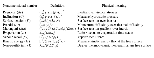
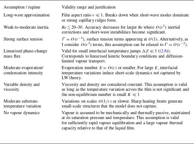
 θ
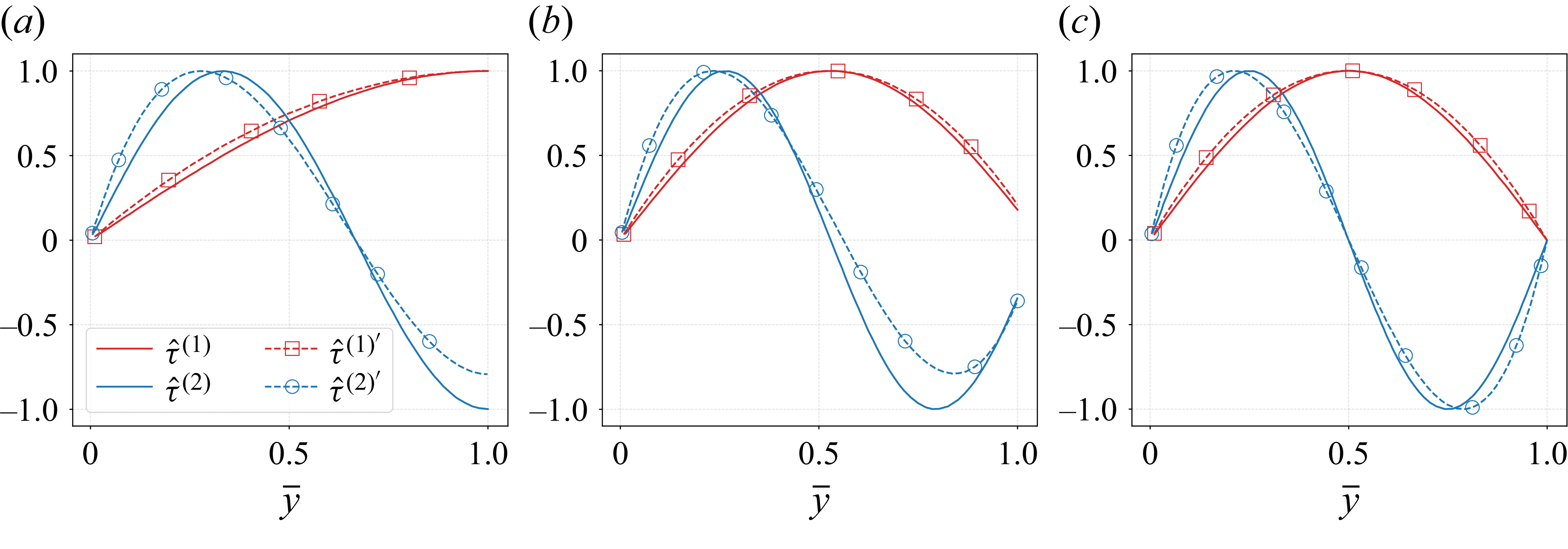
 νk=01
 νk=02
 ν^1
 ν^2
 H¯/K
 10−3
 16
 105
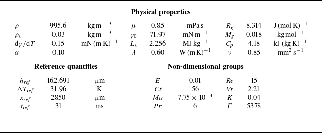
 β=15∘
 T=300
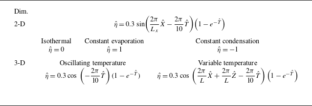
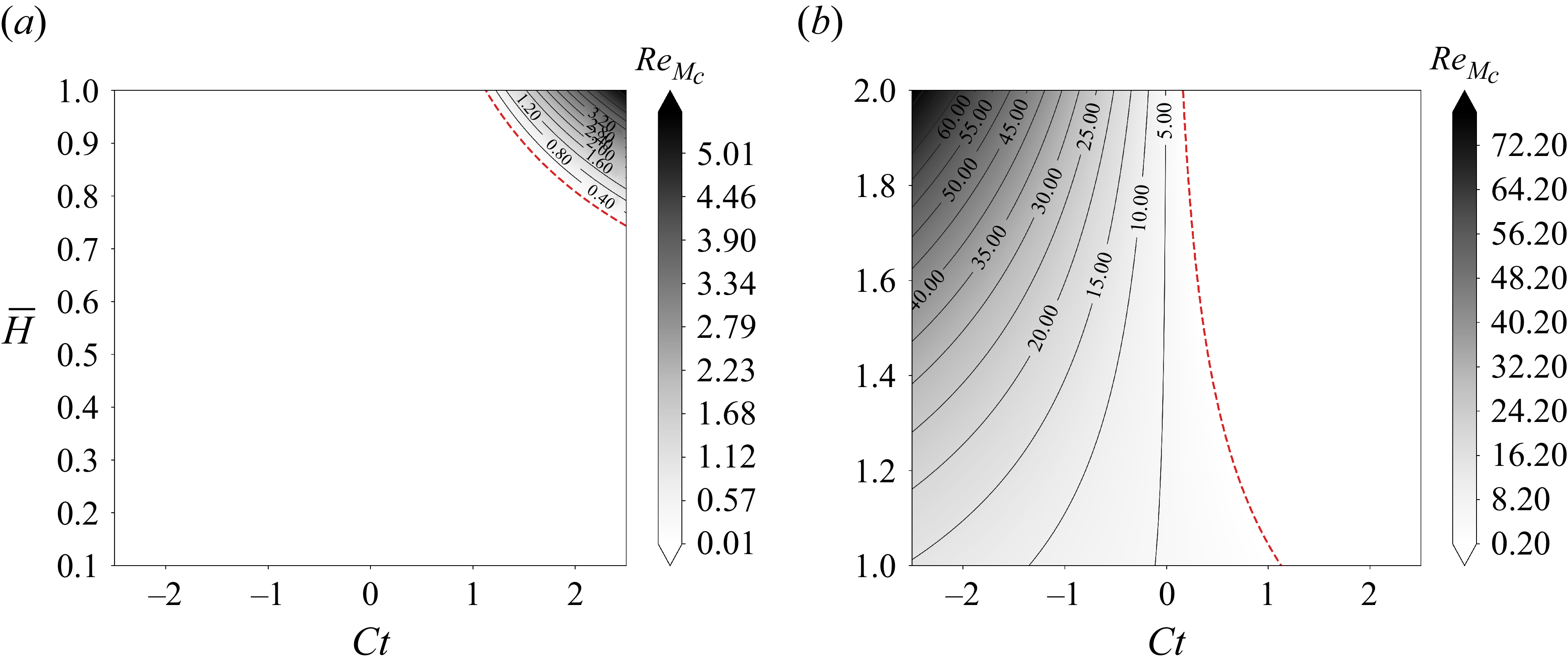
 {Re}Mc
 H¯
 Ct
 Vr=0.5
 η^=1
 η^=−1

 kx,Re
 ωi
 kx
 Re=20,40,60,80
 Γ=1000
 H¯=1

 Re,kx)
 kz=0
 Ma=10
 Vr=4
 Ma=Vr=0
 β
 ∘
 ∘

 ωi
 c
 kx
 kz=0
 H¯=1
 Vr=4
 Ma=10
 Ma=Vr=0
 β
 π/2
 π/6
 Re=10

 Ma
 kz
 Re=0.1
 Pr=7
 K=0.01
 Γ=1000
 β=90∘
 Vr
 H¯=1
 ωi
 kz
 Ma=1
 Vr=2
 Vr=0

 β=π/12
 Π=0
 Γ=1000
 Pr=7
 Vr=4
 K=0.01
 E=0.1
 η^=1
 Ma=10
 t^
 0.3t^d
 0.6t^d
 t^=0

 ωi
 c
 H¯
 β=π/12
 Re=20
 Π=0
 Γ=1000
 Pr=7
 Vr=4
 K=0.01
 E=0.1
 Ma=10
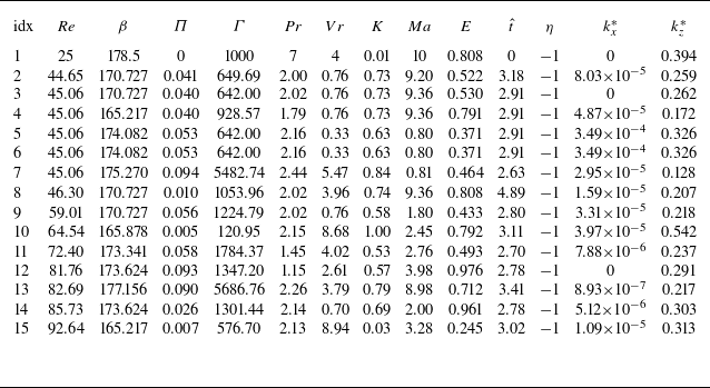
 β
 η^
 t^
 ωi∗
 kz∗≠0
 Re

 β=π/12
 Π=0
 Γ=1000
 Pr=7
 Vr=2
 K=0.01
 Re=0.1

 (β,Re)

 ωix∗
 ωiz∗
 kx∗
 kz∗
 Re=80
 β
 ωi
 kx,kz
 β
 170∘
 174∘
 ωi∗


 y

 h^min
 ⟨J^⟩Ω
 η^=0.3
 η^=−0.3

 h^

 h^
 η^=0.3
 η^=−0.3

 y


 Open access

