DRAWING CONCLUSIONS FROM EVIDENCE

We first present an example to help the reader crystallize the dimensions of judgment on which researchers may differ when drawing conclusions about substantive significance. We think this is easiest to do using an analogy between an intuitively compelling (but evidence-based) decision and a more ordinary social scientific decision that a researcher might make in day-to-day work.

Figure 1 illustrates this analogy. Let us assume that researchers develop an interesting new drug that can reliably produce any level of weight loss desired by the user. But researchers suspect that a fatal cancer might be a side effect of the drug. Figure 1a depicts a hypothetical posterior belief distribution of the change in cancer probability based on a series of (imagined) studies; we denote this change in cancer probability r. The distribution is centered over a 25 percent increase in a subject’s chance of developing cancer, but the 95 percent confidence interval is [−48 percent; 98 percent] corresponding to a one-tailed p-value of about 0.25. That is, the relationship between this drug and cancer is statistically insignificant.

Fig. 1

Hypothetical evidence-based decisions (a) Would you take this weight loss drug? (b) Would you believe that non-democracies have more civil wars than democracies?

Would you take this drug?

A rational chooserFootnote ⁴ would consider the potential consequences of taking the drug vs. not taking the drug under each of the possible states of the world––each of the possible values of $$\partial \Pr ({\rm cancer})/\partial \:{\rm take}\;{\rm drug}=r$$ under the posterior––and then determine whether taking the drug has a positive expected utility:

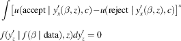
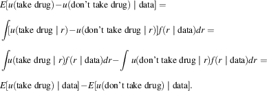$$\eqalignno{ & E[u({\rm take}\;{\rm drug})\!-\!u({\rm donʼt}\;{\rm take}\;{\rm drug})\mid{\rm data}]= \cr & \mathop{\int} \!\!\left[ {u({\rm take}\;{\rm drug}\mid r)\!-\!u({\rm donʼt}\;{\rm take}\;{\rm drug}\mid r)} \right]f(r\mid{\rm data})dr= \cr & \mathop{\int} \!\!\!u({\rm take}\;{\rm drug}\mid r)f(r\mid{\rm data})dr\!-\!\mathop{\int} u({\rm donʼt}\;{\rm take}\;{\rm drug}\mid r)f(r\mid{\rm data})dr=^{} \cr & E[u({\rm take}\;{\rm drug})\mid{\rm data}]\!-\!E[u({\rm donʼt}\;{\rm take}\;{\rm drug})\mid{\rm data}]. $$

The decision to choose to take the drug when the expected utility (in Equation 3) is greater than zero, and to not take it otherwise, is the Bayes decision rule:

$$\eqalignno{ & d(x)={\rm take}\;{\rm drug}\;{\rm if}\;\:E[u({\rm take}\;{\rm drug})\mid x]> E[u({\rm donʼt}\;{\rm take}\;{\rm drug}) \!\mid x] \cr & \:{\rm donʼt}\;{\rm take}\;{\rm drug}\;{\rm otherwise} $$

where we let x signify the data. The rule associates each state of the world $$f(r\mid\:{\rm data}\:)$$ with an optimal Bayes action that maximizes expected benefit (French and Insua Reference French and Insua2000, 148). Uncertainty about the actual effect of the drug plays a role in the decisionFootnote ⁵ through $$f(r\mid\:{\rm data}\:)$$ . This Bayes decision rule d(x) is optimal in that it minimizes the Bayes risk, the expected loss in utility $$l({\bullet})=\!-\!u({\bullet})$$ from a decision rule averaging over both sampling variation in the data and the prior distribution of r:

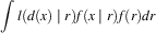
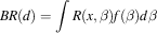
$$BR(d)=\mathop{\int} \left[ {\mathop{\int} l\left( {d(x)\mid r} \right)f(x\mid r)dx} \right]f(r)dr.$$

Summarily, it is rational to commit to following the Bayes decision rule because it maximizes utility (equivalent to minimizing loss) given all sources of uncertainty in our empirical evidence.Footnote ⁶

While there may be disagreements over the quality of the evidence, we set them aside to focus on differences in interpretation of the evidence. These differences in judgment presumably come through the utility function u. For example, some people may be more loss averseFootnote ⁷ than others; they would presumably be less willing to gamble on the possibility of getting cancer in order to lose weight. The difference on this dimension is in how people weight the relative value of forsaking a gain if the drug is harmless compared to the value of avoiding a loss if it causes cancer. People may also differ in their absolute valuation of a cancer outcome: a small but completely certain increase in cancer incidence (say, 0.5 percent) might be negligible to some people compared to the benefit of weight loss, while others may consider this incidence extremely meaningful from a personal or public health perspective.

Now consider another decision: should we act on the conclusion that democratic states are less likely to suffer a civil war compared to non-democracies, or treat democracies as being at least equally likely to experience a civil war? Based on the (hypothetical) evidence shown in Figure 1b, the posterior distribution of the difference in intrastate conflict probability (which we denote as β) is the same as the distribution of the difference in cancer probability from Figure 1a. As before, a rational chooser should determine whether there is a greater scientific (or policy) benefit to acting on the conclusion that democracies are less susceptible than non-democracies to civil war, or to treating democracies as at least equally susceptible, based on the available evidence:

$$\eqalignno{ & E[u({\rm treat}\;{\rm as}\;{\rm unequal})\!-\!u({\rm treat}\;{\rm as}\;{\rm equal})\!\mid {\rm data}]= \cr & \mathop{\int} \left[ {u({\rm treat}\;{\rm as}\;{\rm unequal}\mid\beta )\!-\!u({\rm treat}\;{\rm as}\;{\rm equal}\mid\beta )} \right]f(\beta \mid{\rm data})]d\beta . $$

More generally, we could write this decision as:

$$\eqalignno{ & E[u({\rm act}\;{\rm on}\;{\rm alternative})\!-\!u({\rm act}\;{\rm on}\;{\rm null})\!\mid {\rm data}]= \cr & \mathop{\int} \left[ {u({\rm act}\;{\rm on}\;{\rm alternative}\mid\beta )\!-\!u({\rm act}\;{\rm on}\;{\rm null}\mid\beta )} \right]f(\beta \mid{\rm data})]d\beta , $$

where the alternative hypothesis is that democracies are less prone to civil war, and the (default) null hypothesis is that they are at least equally prone to civil war. Of course, we would not expect $$u({\rm act}\;{\rm on}\;{\rm alternative}\mid\beta )\!-\!u({\rm act}\;{\rm on}\;{\rm null}\mid\beta )$$ to be the same for this decision as for the decision to take the weight loss drug. But the considerations involved in shaping the judgment are similar: (1) how much does the scientist weight the consequences of falsely acting on the alternative against the consequences of falsely acting on the null, and (2) how large must democracies’ advantage in civil war susceptibility be before it merits scientific and political attention?

Rather than argue for a particular answer to these questions, our goal is to determine whether researchers with a variety of different standards would make the same decision according to Equation 4. We must still choose a utility function, but ideally it will be one that can fairly represent a variety of standards for evaluating evidence. In particular, it should be able to represent a continuum of relative valuations for false positives (mistakenly acting on the alternative hypothesis) and false negatives (mistakenly acting on the null hypothesis).

QUANTIFYING THE DECISION: UTILITY, LOSS AVERSION AND DECISION RULE

The functional form of $$u({\rm act}\;{\rm on}\;{\rm alternative}\mid\beta )\!-\!u({\rm act}\;{\rm on}\;{\rm null}\mid\beta )$$ is the encapsulation of scientific judgment in this framework, and there is no universally correct choice. Recall that our objective is to find whether different standards of judgment would lead to the same conclusion about the substantive significance of an empirical result. Thus the precise choice of functional form is less important than its ability to approximate a diversity of preferences about (1) the trade-off between false positives and false negatives, and (2) the minimum effect size required for substantive significance. We suggest a function that is simple, yet flexible enough to adapt to varying decision contexts and the preferences of different researchers. We do not claim that it is unique or superior to all possibilities, but it meets our stated criteria well and provides some inferential benefits that we explore below.

For the decision of whether to act on the conclusion that the relationship between two variables (such as democracy and intrastate conflict) is positive and large enough to be scientifically or politically important, we focus on a loss-averse utility function:

$$u({\rm act}\;{\rm on}\;{\rm alternative}\mid\beta ,\gamma ,c)\!-\!u({\rm act}\;{\rm on}\;{\rm null}\mid\beta ,\gamma ,c)=\gamma ^{{\!-\!{\rm sign}(\beta \!-\!c)}} \left[ {\beta \!-\!c} \right].$$

Here, the alternative is the conclusion that $$\beta \geq c$$ and the null is the conclusion that β<c.Footnote ⁸ This utility function is depicted in Figure 2 for c=0. In terms of our previous democracy-conflict example, this is equivalent to saying that a non-democracy’s chance of suffering a civil conflict is at least c more than a democracy’s. Utility is gained in proportion to distance from the threshold for substantive significance c. With all else held equal (that is, in a single decision context), bigger relationships are more substantively important than small ones, and the smallest positive relationship worth paying attention to is of size c. That is, the consequences of accepting this conclusion are linearly related to the size of the difference. γ is a parameter that describes the valuation ratio for correct and incorrect decisions, or the degree of loss aversion that the researcher exhibits; it is the degree of kink in the function in Figure 2. Downward kinks indicate that correctly acting on the alternative is less important than incorrectly doing so (a false negative is less damaging than a false positive), and correspond to γ>1. Upward kinks indicate that correctly acting on the alternative is more important than incorrectly doing so (that is, a false positive is less damaging than a false negative) and correspond to $$\gamma \in (0,1)$$ .

Fig. 2

Loss-averse utility functions

The Bayes decision rule under this utility framework is to act on the alternative hypothesis ( $$\beta \geq c$$ ) whenever:

$$\mathop{\int} \!\!\!\gamma ^{{\!-\!{\rm sign}(\beta \!-\!c)}} \left[ {\beta \!-\!c} \right]f(\beta \mid{\rm data})d\beta &#x0003E; 0$$

and to act on the null hypothesis otherwise.Footnote ⁹ There are two unknowns, γ and c, which correspond to the two variable dimensions of scientific judgment that we laid out at the start. By determining the c* that solves:

$$\mathop{\int} \!\!\gamma ^{{\!-\!{\rm sign}(\beta \!-\!c^{{\vskip 2.6pt{\tf="PPLbody_Roman"\char"2A}}} )}} \left[ {\beta \!-\!c^{{\vskip 2.6pt{\tf="PPLbody_Roman"\char"2A}}} } \right]f(\beta \mid{\rm data})d\beta =0,$$

we can sketch a γ/c * curve over which the researcher is indifferent to acting on the alternative hypothesis given γ and c*.

COMPUTING c* AND CHOICE OF A PRIOR

The vast majority of mainstream statistical software packages can compute the γ/c* curve using add-on packages. We have developed software for R and Stata that, when given a γ, will compute a c* immediately after a linear regression or other generalized linear model. The software will also determine c* when given manually entered information from a published table (without the accompanying dataset).Footnote ¹⁰

The software package assumes a truncated uniform prior distribution f(β) on the interval defined by $$\hat{\beta }\pm8\hat{\sigma }$$ . This structure assumes minimalistic knowledge of the underlying parameters before examining a dataset. It also allows for a Bayesian interpretation of frequentist results: for the classical linear regression model, $$f(\beta \mid{\rm data})$$ takes a multivariate t distribution with n−k degrees of freedom (Gelman et al. Reference Gelman, Carlin, Stern and Rubin2003, 355–7). The software therefore uses a t distribution for the posterior when computing c* in these cases. For generalized linear models with this prior estimated via maximum likelihood, $$f(\beta \mid{\rm data})$$ is asymptotically normal as $$n\to\infty$$ (Gelfand and Ghosh Reference Gelfand and Ghosh2000, 4–8), and therefore the software uses the normal distribution in these instances.

Computing c* is a matter of finding the roots of Equation 7 (or the equivalent for an alternative utility function). This class of problem is already solved via iterative maximization algorithms, such as Newton-Raphson,Footnote ¹¹ but we are required to compute an integral at each iteration because we are calculating an expected value rather than a maximum or modal value. For results with a t-distributed or normally distributed posterior, we can use standard quadrature approaches to quickly compute the integral for each step of the maximization process.

Some analysts may wish to impose stronger prior beliefs, which will change the distribution of $$f(\beta \mid{\rm data})$$ . If the prior is conjugate with the posterior, the analyst must replace the multivariate t or normal distribution with the appropriate posterior distribution before calculating c*. For more exotic posteriors, where $$f(\beta \mid{\rm data})$$ is difficult to analytically express, an approximation can be computed via Markov Chain Monte Carlo methods, stored, and then used in the integration of Equation 7.

WHAT DOES A SUBSTANTIVELY ROBUST (OR NON-ROBUST) FINDING LOOK LIKE?

Figure 3b sketches the γ/c* curve for our democracy and war example using Equation 7. The relevant question is: can we conclude that non-democracies are susceptible to a greater risk of civil war on the basis of the evidence of Figure 1b? Our answer is that a researcher would accept an increased civil war probability under the point on the curve corresponding to his/her γ. Equivalently, a researcher would decide how large a relationship had to be before it was scientifically or politically meaningful and how loss averse s/he is, then find the appropriate point in Figure 3b and make the decision indicated. For example, a person who weighted false positives and false negatives equally (with γ=1) would be willing to act on the belief that non-democracies are ≤25 percent less likely to experience civil war than comparable non-democracies. But a person who valued false positives four times as much as false negatives $$(\gamma =\sqrt 4 =2)$$ would only be willing to act on a≤5 percent difference in civil war risk, and a person who valued false positives even more highly would always act on the null (of a nonexistent or negative relationship). In short, the association between democracy and civil war risk (in this hypothetical example) is not robust to reasonable ranges of variation in standards for interpreting evidence. It is not necessarily important for a researcher to know his or her own γ, but simply to acknowledge that a community of people with reasonable variation in how much they valued false positives more highly than false negatives would not agree on the substantive significance of the relationship between democracy and civil war risk.

Fig. 3

Substantive robustness of inference from Figure 1 (a) Drugs and cancer probability (Figure 1a) (b) Democracy and war probability (Figure 1b)

By contrast, the conclusion that we should not take the weight loss drug (for fear of cancer risk, as shown in Figure 1a) is quite robust. Figure 3a sketches the γ/c* curve for this example; the key difference, compared to the democracy/war example, is that $$\gamma \in [0,1]$$ would be appropriate for a person who was much less concerned about mistakenly acting on the alternative (accidentally concluding that the drug causes cancer when it does not, and therefore not taking the drug when it would be beneficial) compared to mistakenly acting on the null (mistakenly believing that the drug does not cause cancer when it actually does, and therefore taking the drug when it increases one’s likelihood of developing cancer). For this reason, even wide variation in standards for the interpretation of evidence produces the conclusion that there is a large and substantively meaningful link between the drug and cancer risk. It is not so important for any particular person to locate their personal value of γ, but simply to acknowledge that it lies somewhere between 0 and 1 (that is, that they value false negatives more highly than false positives in some measure) and that people with diverse preferences in this domain would avoid taking the drug.

We think these examples illustrate the value of focusing on the robustness of substantive significance to different standards rather than on any particular judgment of substantive significance. Figure 3 makes clear that comparatively small differences in loss aversion (that is, aversion to falsely rejecting the null) can sometimes (but not always) translate into large differences in the assessment of substantive significance. Aggressive researchers who are relatively indifferent to false positives (γ≈1) would conclude (based on our hypothetical evidence) that there is a substantively significant association between democracy and civil war probability as long as they thought that a 25 percent increase in war probability was meaningful. More cautious researchers, who weight false positives as more damaging (γ≳2.5), would never draw this conclusion. These are rather wide differences in judgment that relate to incommensurable differences in scientific viewpoint. Consequently, we think that arguing for a universally acceptable γ, let alone a universally acceptable form for $$u({\rm act}\;{\rm on}\;{\rm alternative})\!-\!u({\rm act}\;{\rm on}\;{\rm null})$$ , is probably hopeless in the context of academic research. By focusing on the breadth of preferences for which a result is substantively significant, rather than on any particular preference, we sidestep the knotty question of “whose judgment is correct?” in favor of the more readily answerable “would this evidence satisfy most researchers?” For the example of the weight loss drug, researchers with a wide variety of standards would all agree that the drug should not be taken.

Substantive Robustness Assessment Can Improve the Quality of Published Results

When it comes to statistical hypothesis testing, we determine that it is advantageous to require a result to be both substantively robust and statistically significant in order to be scientifically notable, compared to requiring statistical significance alone. Aside from the theoretical and descriptive value of assessing the substantive robustness of results, requiring a statistical relationship to be statistically significant and substantively robust before rejecting the null hypothesis (of no relationship) results in a more powerful test (a greater probability of rejecting false null hypotheses) at any given size (probability of rejecting correct null hypotheses). This advantage accrues to the combined procedure because results that are statistically significant but substantively fragile frequently occur when the null hypothesis is true, but rarely occur when the alternative is true. The upshot is that a researcher using our procedure will draw fewer mistaken conclusions than a researcher who just uses statistical significance testing.

To demonstrate, we conduct a simulation to calculate the rate at which the null hypothesis is rejected using two different procedures:

1. 1. statistical significance: reject if two-tailed p≤α.

2. 2. combined statistical significance and substantive robustness: reject if

   1. (a) result is statistically significant (two-tailed p≤α), and

   2. (b) $$c^{{\vskip 2.6pt{\tf="PPLbody_Roman"\char"2A}}}\!&#x0003E;\!0$$ for γ=2.

For the second procedure, we choose a relatively small γ=2 in order to ensure a very minimal bar for substantive robustness. We also set the critical threshold for substantive acceptability to c*>0, the smallest (and easiest-to-pass) threshold for a test of a positive relationship, for the same reason. In short, a result will be judged substantively robust in this simulation if someone with γ ≤2 would be willing to act on the alternative hypothesis, even for a very small relationship size.

Our simulation uses a linear DGP:

$$y=2+\beta _{x} x+u.$$

In all simulations, $$u\sim\Phi (\mu =0,\:\sigma =0.5)$$ . We use three values of β _x: β _x=0.75 (a “large effect” more easily detected by statistical tests), β _x=0.25 (a “small effect” harder to distinguish from noise) and β _x=0 (the null hypothesis). For each value of β _x, we conduct 1,000 simulations with datasets of size n=100 each. We then repeat these simulations for values of α (the critical value for the statistical significance test) between 0.005 and 0.2 to get a range of false positive rates. The results are depicted in Figure 4.

Fig. 4

Size/power analysis for statistical significance testing, with and without substantive robustness checking (a) Large effect (b) Small effect

Figure 4a plots the proportion of the time that a test procedure rejected the null when β _x=0 on the x-axis, and the proportion of the time the test rejected the null when β _x=0.75 on the y-axis. Figure 4b plots the same relationship, but with the null rejection rates for β _x=0.25 on the y-axis. Ideal performance would mean a completely $$\Gamma $$ -shaped curve—an estimator that could achieve a 100 percent true positive rate at a 0 percent false positive rate. Better testing procedures are those that have larger true positive rates for every false positive rate: they can correctly reject false null hypotheses without accidentally rejecting true null hypotheses. As the figure shows, combining statistical significance with a very minimal evaluation of substantive acceptability––a mildly loss-averse researcher (γ=2) must be willing to accept an effect of any magnitude––improves the power of the test at every size. The performance gap varies according to the nature of the DGP and the α value of the statistical significance test, but combined testing improves power by as much as 10 percentage points in our simulations (for a false positive rate ≈10 percent in Figure 4b).

We also find support for a very useful rule of thumb: if a result is statistically significant but not substantively meaningful (c*=0 when γ=2), in all likelihood the null hypothesis is the correct one. The relevant Bayesian formula for beliefs in this situation is:

$$\eqalignno{ &#x0026; \Pr ({\rm null}\;{\rm false \mid stat}{\rm .}\;{\rm sig}{\rm .,}\;{\rm sub}{\rm .}\;{\rm not}\;{\rm robust})= \cr &#x0026; {{\Pr ({\rm result}\;{\rm pattern\mid null}\;{\rm false)Pr(null}\;{\rm false})} \over {\Pr ({\rm result}\;{\rm pattern\mid null}\;{\rm false})\Pr ({\rm null}\;{\rm false})+\Pr ({\rm result}\;{\rm pattern\mid null}\;{\rm true})\Pr ({\rm null}\;{\rm true})}}. $$

But in our simulations, there were no occurrences in which the result was statistically significant (α=0.05) but substantively not robust (c*=0 when γ=2) when the null was false; all of the false negatives in the combined test were cases in which the result was substantively (but not statistically) significant. To ensure the robustness of this finding, we repeat our simulations for β _x=0.25 with greater noise in the DGP ( $$u\sim\Phi (\mu =0,\:\sigma =2.5)$$ ), making false negatives much more likely. We still find that this pattern of results only occurred 1.5 percent of the time under the null hypothesis, leading to an updated belief of:

$$\Pr ({\rm null}\;{\rm false}\mid{\rm stat}{\rm .}\;{\rm sig}{\rm .,}\;{\rm sub}{\rm .}\;{\rm not}\;{\rm robust})={{0.015\,{\vskip 2.6pt{\tf="PPLbody_Roman"\char"2A}}\,0.5} \over {0.015\,{\vskip 2.6pt{\tf="PPLbody_Roman"\char"2A}}\,0.5+0.028\,{\vskip 2.6pt{\tf="PPLbody_Roman"\char"2A}}\,0.5}}=0.349,$$

where we determine $$\Pr ({\rm result}\;{\rm pattern}\mid{\rm null}\;{\rm true})=0.028$$ by repeating our simulations for β _x=0 with $$u\sim\Phi (0,\:2.5)$$ . Even under a prior probability of 50 percent that the null is false, the posterior probability that the null is false is only 34.9 percent––nowhere close to conventional significance levels in a hypothesis test. Summarily, our simulation evidence indicates that statistically significant, but substantively non-robust, results are almost surely ascribable to chance.

ASSESSING THE SUBSTANTIVE ROBUSTNESS OF EXISTING RESEARCH

As a technical matter, it is straightforward to assess the substantive robustness of existing research using our technique. We demonstrate using two recently published articles from prominent general interest journals in political science. These examples allow us to show how quantitatively assessing substantive robustness helps refine our interpretation of the results. They also illustrate how our techniques are applied to models with complex marginal effects, such as those from models with interaction (product) terms, where these substantively important quantities are a combination of multiple coefficient estimates and cannot be read directly off of a coefficient table. Finally, we provide documented code for each of these examples, which readers can use to replicate our results or adapt for use in their own inference problems.Footnote ¹²

Applied Example: Clinton (Reference Clinton2006)

First, we will re-examine some of the critical results from Joshua Clinton’s Reference Clinton2006 article on representation in Congress in the Journal of Politics (Clinton Reference Clinton2006). In this article, Clinton examines the relationship between a survey-based ideology measure of residents of American congressional districts in the year 2000 and legislator ideal points estimated on the basis of voting records.Footnote ¹³ In his ordinary least squares (OLS) regression analysis, he finds that there is a positive relationship between the conservatism of a Republican legislator’s voting record and the degree of conservatism expressed by his/her Republican constituents. The same relationship exists between a Republican legislator’s record and his/her Democratic constituents’ ideology. The conservatism of Democratic legislators’ records, by contrast, is associated with the conservatism of their Republican, but not Democratic, constituents.

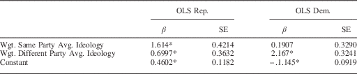
While Clinton uses both OLS regression and an errors-in-variables regression designed to correct for measurement errors, we focus on the OLS results in this replication.Footnote ¹⁴ We perform the same OLS regression that Clinton ran, the results of which are shown in Table 1. We then calculate a substantive robustness plot for all four effects: the effect of Republican and Democratic constituents on Republican legislators and on Democratic legislators. These plots are shown in Figure 5.

Fig. 5

Substantive robustness assessment for constituent influence on “key votes” in Congress, from Clinton (Reference Clinton2006) (a) Republican constituents’ influence on Republican legislators (b) Democratic constituents’ influence on Republican legislators (c) Republican constituents’ influence on Democrat legislators (d) Democratic constituents’ influence on Democrat legislators

Table 1

Constituent Influence on “Key Votes” in Congress (Table 3 from Clinton Reference Clinton2006)

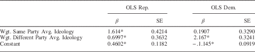
Note: dependent variable=legislator ideology score from Clinton, Jackman and Rivers (Reference Clinton, Jackman and Rivers2004). N=222 (Republicans) and 210 (Democrats). R ²=0.09 (Republicans) and 0.26 (Democrats). *indicates statistical significance, α=0.05 (one-tailed).

In Clinton’s analysis, Republican and Democrat constituents’ ideologies have a statistically significant relationship with their Republican legislators’ voting records, but only Republican constituents’ ideology is related to Democrat legislators’ voting records. Substantively speaking, however, the robustness of these results varies. Republican constituents’ ideology seems to have a reasonably robust relationship with both Democrat and Republican legislators’ voting records (Figures 5a and 5c): even researchers who value false positives 36 times more than false negatives (γ=6) would act on the belief that the coefficient ≳1. With a coefficient of 1, a one standard deviation change in constituent ideology is predicted to move a Democratic legislator at the 50th percentile of his/her party’s ideology to the 57th percentile. The effect on Republican legislators is smaller, but still politically significant: a one standard deviation change in Republican constituents’ ideology is predicted to move a Republican legislator at the 50th percentile of his/her party’s ideology to the 53rd percentile. Visually, we can see that these results are substantively robust, because the range of acceptable coefficients is large across a very wide swath of loss aversion coefficients γ.

The relationship between Democrat constituents’ ideology and legislators’ voting records is much less robust. This may not be immediately clear from looking at the coefficients in Table 1. For instance, the 90 percent confidence interval for Democratic constituents’ effect on Republican legislators is [0.1, 1.3]. This estimate indicates considerable uncertainty about this relationship, but it also firmly excludes the null and includes the possibility of a substantively large relationship. But as Figure 5b shows, a community of heterogeneous researchers would tend to agree on a coefficient of less than or equal to about 0.2––quite close to the left boundary of the 90 percent confidence interval. A coefficient of this size implies that a one standard deviation change in Democrat constituent ideology moves a Republican legislator at the 50th percentile of his/her party’s ideology to the 52nd percentile. That is a reasonably small relationship, probably politically ignorable. We conclude that the relationship between Democrat constituents and Republican (or Democratic) legislators is not robust to different standards of substantive judgment. Visually, the non-robustness of these relationships is visible because the range of acceptable coefficient sizes is close to zero (or actually zero) for even modest values of loss aversion γ.

Given our earlier simulation results, which indicated that false positives are minimized by accepting only those results that are substantively robust and statistically significant, we are led to conclude that Clinton’s evidence does not support a link between Democrat constituents’ ideology and the voting records for legislators of either party. Indeed, when estimating an errors-in-variables regression on the same data, Clinton comes to the same conclusion (but on the basis of statistical significance).

Applied Example: Brambor, Clark and Golder (Reference Brambor, Clark and Golder2006)

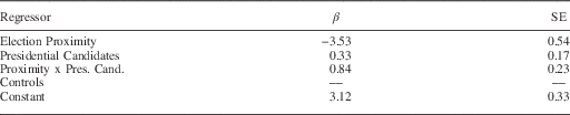
In an influential article, Brambor, Clark and Golder (Reference Brambor, Clark and Golder2006, hereafter BCG) describe the importance of interpreting interaction terms substantively, and provide tools and techniques for informative interpretation. These tools and techniques are readily adapted to substantive robustness assessment using our technique. In one example, BCG present a graphical method of presenting marginal effects from linear models with interaction terms. Their example comes from Clark and Golder (Reference Clark and Golder2006), a model of the relationship between presidential elections and legislative fragmentation (the number of parties in the legislature). The model is listed in Table 2; note that the relationship between the proximity of presidential elections and the number of electoral parties in the legislature is contingent on the number of presidential candidates.

Table 2

The Impact of Presidential Elections on the Effective Number of Electoral Parties (Table 1 from Brambor, Clark and Golder Reference Brambor, Clark and Golder2006)

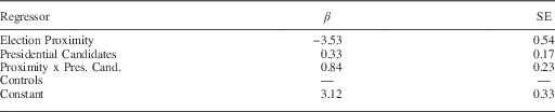
Note: OLS model of the number of electoral parties in the legislature. Standard errors are clustered on country. R ²=0.25, N=602.

To test hypotheses about the marginal effect of presidential elections on legislative fragmentation, BCG recommend constructing a plot like the one in Figure 6a, which shows this marginal effect and its 95 percent confidence interval for different numbers of presidential candidates. Mathematically, the marginal effect shown in the figure is:

$${{\partial \,\#\,{\rm candidates}} \over {\partial \:\;{\rm presidential}\;{\rm elections}}}=\beta _{{proximity}} +(\beta _{{prox{\vskip 1.6pt{\tf="PPLbody_Roman"\char"2A}}cand}} \,{\vskip 3pt{\tf="PPLbody_Roman"\char"2A}}\,\#\,{\rm candidates})$$

and therefore a combination of multiple coefficients from the regression. In Figure 6a, we augment this assessment of statistical significance with a substantive robustness assessment. Specifically, we use our software to determine c* for each number of presidential candidates using the loss averse utility function from Equation 5 and a variety of different loss aversion coefficients γ.Footnote ¹⁵ The shaded regions indicate the marginal effect sizes that could be acted upon by researchers with the corresponding level of loss aversion γ. The wider the shaded range, the more robust is the judgment of substantive significance.

Fig. 6

Robustness assessment for the marginal effect of proximate presidential elections on number of electoral parties in the legislature (Figure 3 from Brambor, Clark and Golder Reference Brambor, Clark and Golder2006) (a) Statistical significance assessment (b) Substantive robustness assessment

As the figure shows, when the number of presidential candidates is small (between 0 and ≈1.5), there is a very robust negative relationship between presidential elections and the number of electoral parties. Even researchers who are extremely averse to false positives (γ>20, valuing a false positive 400 times more than a false negativeFootnote ¹⁶) should conclude that the number of legislative parties participating in an election shrinks by ≈1 when concurrent presidential elections are held (compared to legislative elections held precisely in between presidential terms, such as a US mid-term election). To reduce the interpretation to simple visual terms, there is a broad swath of the marginal effect space that is shaded at a very high level of γ, indicating that even researchers who are extremely averse to false positives would act on the alternative hypothesis of a large marginal effect. In short, researchers with a wide variety of standards for interpreting evidence would accept a large relationship between presidential elections and the number of electoral parties in the legislature.

This negative relationship becomes less robust as the number of presidential candidates grows. When there are three presidential candidates, for example, researchers who are even moderately averse to false positives (γ>4) would act on the null that there is no relationship at all. Those who are reasonably indifferent between Type I and II errors (γ≤2, valuing false positives 4 times as much as false negatives) would be willing to act on the belief that a reduction of ≈1 party occurs when presidential elections are concurrent. These same researchers would also accept that there is a positive relationship between the number of legislative parties and the fact of concurrent presidential elections when there are a very large number of presidential candidates competing for office (≈6). In visual terms, only a small portion of the marginal effect space is shaded, and only for comparatively small γ; this indicates that many researchers would not conclude that there is a substantively significant relationship (that is, they would act on the null).

The pattern of substantive findings––a negative relationship between legislative parties and proximate presidential elections when the number of presidential parties is low, and no relationship otherwise––is consistent with the statistical significance findings depicted in Figure 6a, and with Clark and Golder’s theoretical hypothesis. Based on our earlier simulations, we therefore have a great deal of confidence in the robustness of this finding.