1 Introduction
Planar multipolar flows are a class of flows created by a fluid confined between two thinly spaced parallel plates and driven by a set of discrete inlets and outlets connected to either plate. They occur in many devices, including radial diffusers (Woolard Reference Woolard1957; Moller Reference Moller1966), hydrostatic thrust bearings (Osterle & Hughes Reference Osterle and Hughes1958; Hunt & Torbe Reference Hunt and Torbe1962; Savage Reference Savage1964; Jackson & Symmons Reference Jackson and Symmons1965a ,Reference Jackson and Symmons b ), radial flow nozzles (Hagiwara Reference Hagiwara1962), in the context of radial fingering in Hele-Shaw cells (Richardson Reference Richardson1972, Reference Richardson1981; Paterson Reference Paterson1981, Reference Paterson1985; Howison Reference Howison1986; Daccord, Nittman & Stanley Reference Daccord, Nittman and Stanley1986; Chen Reference Chen1987, Reference Chen1989; Rauseo, Barnes & Maher Reference Rauseo, Barnes and Maher1987), in the domain of injection moulding (Kamal & Kenig Reference Kamal and Kenig1972a ,Reference Kamal and Kenig b ; Stevenson Reference Stevenson1976) and in the field of groundwater, hydrocarbon or geothermal heat recovery (Koplik, Redner & Hinch Reference Koplik, Redner and Hinch1994; Kurowski et al. Reference Kurowski, Ippolito, Hulin, Koplik and Hinch1994; Zhang & Koplik Reference Zhang and Koplik1997). Planar multipolar flows are also observed in nature; for instance, in the human choriocapillaris, a microvascular bed responsible for the maintenance of the outer part of the sensory retina (Zouache et al. Reference Zouache, Eames, Klettner and Luthert2016). The properties of planar multipolar flows have been applied to study the adhesion and detachment of microbial elements (Fryer, Slater & Duddridge Reference Fryer, Slater and Duddridge1985) and mammalian cells (Goldstein & Di-Milla Reference Goldstein and Di-Milla1996), to cleaning in industrial processes (Detry et al. Reference Detry, Rouxhet, Boulangé-Petermann, Deroanne and Sindic2007, Reference Detry, Deroanne, Sindic and Jensen2009) and to generate a steady non-uniform concentration field in microfluidic devices for biological applications (Qasaimeh, Gervais & Juncker Reference Qasaimeh, Gervais and Juncker2011).
Planar multipolar flows are characterised by three distinct regions: an axisymmetric radial entry (or exit) flow in the pipe region, a turning region and a channel flow region. Axisymmetric radial channel flows form a well-studied class of problems; however, few studies have considered the geometry that characterises them in its entirety. Previous work on the turning region include three-dimensional axisymmetric stagnation point flows as they may be used to approximate the flow close to the wall opposite to the pipe. Analytical and numerical solutions for this type of flows (Homann Reference Homann1936; Howarth Reference Howarth1951; Stewart & Prober Reference Stewart and Prober1962; Gersten & Körner Reference Gersten and Körner1968; Gersten Reference Gersten1973) and heat or mass transfers (Stewart & Prober Reference Stewart and Prober1962; Libby Reference Libby1967; Gersten & Körner Reference Gersten and Körner1968; Gersten Reference Gersten1973) have been formulated for incompressible and compressible fluids and various flow regimes, geometries and boundary conditions. Moller (Reference Moller1966) investigated the effect of a bend in the inlet on the pressure field in the turning region when the flow is turbulent, with the aim of minimising pressure losses. Numerical (Chatterjee & White Reference Chatterjee and White1989) and infinite series solutions in the limit of creeping flows (Chatterjee Reference Chatterjee1993) showed that the flow field in the turning region is governed by the Reynolds number imposed at the pipe (
 $Re_{p}$
) and the ratio between the channel thickness and the pipe radius (
 $\unicode[STIX]{x1D6F6}$
). Chatterjee & White (Reference Chatterjee and White1989) found that flow separation at the sharp corner occurs for
 $Re_{p}=10$
and
 $\unicode[STIX]{x1D6F6}=2$
. The structure of standing vortices on the upper and lower plates was subsequently studied numerically (Chatterjee Reference Chatterjee2000) and experimentally (Nakabayashi, Ichikawa & Morinishi Reference Nakabayashi, Ichikawa and Morinishi2002) for various values of
 $\unicode[STIX]{x1D6F6}$
and
 $Re_{p}$
. None of the studies focused on the turning region considered heat or mass transfers. They have, however, been investigated in the context of non-uniform impinging jets analytically and experimentally (Scholtz & Trass Reference Scholtz and Trass1970), and numerically (Chatterjee & Deviprasath Reference Chatterjee and Deviprasath2001) for
 $Re_{p}\geqslant 50$
and various ratios between the tube nozzle diameter and the nozzle-to-plate distance.
The majority of axisymmetric channel flow problems have been restricted to the space between the parallel plates. Moller (Reference Moller1963) determined approximate solutions for laminar and turbulent radial pressure distributions for incompressible and compressible flows using the Kármán momentum-integral method and carried out a series of experiments to test them. Their experimental results were later used by Savage (Reference Savage1964) to validate analytical solutions for viscously dominated flows obtained through perturbation and series expansion methods. The effect of fluid inertia on the pressure distribution between the plates was investigated using the momentum-integral method (Livesey Reference Livesey1960), the energy-integral method (Elkouh Reference Elkouh1967) and power series expansions (Hunt & Torbe Reference Hunt and Torbe1962). The latter solution was subsequently corrected by Jackson & Symmons (Reference Jackson and Symmons1965b
), who also showed experimentally that the limit at which inertia could be neglected varied with
 $\unicode[STIX]{x1D6F6}$
. Lee & Lin (Reference Lee and Lin1985) formulated a differential solution for the pressure distribution along the channel. Hagiwara (Reference Hagiwara1962) considered the effect of the inlet length on velocity and pressure distributions using integral methods. By applying series expansion methods to solve the boundary layer equation, Ishizawa (Reference Ishizawa1965) showed that, above a critical (reduced channel) Reynolds number, flow separates from the wall, and that the separation point moves away from the inlet as the Reynolds number is increased. The momentum-integral method (Ishizawa Reference Ishizawa1966) and a numerical solution of the vorticity equation (Raal Reference Raal1978) suggested that this critical Reynolds number was equal to 100 or 60, respectively. Detry et al. (Reference Detry, Deroanne, Sindic and Jensen2009) computed the wall shear stress distribution numerically for
 $0.125\leqslant \unicode[STIX]{x1D6F6}\leqslant 1$
and
 $0\leqslant Re_{p}\leqslant 2000$
and identified four different recirculation regions using numerical and experimental methods. The problem of heat or mass transfer in the channel region was considered analytically by Stevenson (Reference Stevenson1976) to investigate disk filling by injection moulding in the limit where radial diffusion can be neglected. A Newton-type law of cooling with fixed heat transfer coefficient was imposed at the upper and lower walls, and transfers were only considered away from the inlet. Camera-Roda et al. (Reference Camera-Roda, Boi, Saavedra and Sarti1994) investigated heat and mass transfers for Reynolds numbers larger than 10 (experiments were carried out at Reynolds number 450 and 4500) when either parabolic or linear velocity profiles were imposed between the plates and a Dirichlet boundary condition for the concentration field was set on one of the plates; transport in the turning region was not considered. Mukhopadhyay (Reference Mukhopadhyay2009) formulated closed form solutions for heat transfers (for Péclet numbers varying between 1 and 100) for slug and fully developed creeping flows when a Dirichlet condition was imposed at both plates by neglecting radial diffusion. They found that the heat transfer coefficient converges to 4.93 for slug flows and 3.77 for fully developed creeping flows. Their results were in good agreement with experimental data from Prata, Pilichi & Ferreira (Reference Prata, Pilichi and Ferreira1995), who considered radial diffusers with varying
 $\unicode[STIX]{x1D6F6}$
at Reynolds numbers between 600 and 4595.
Multipolar configurations composed of more than one pipe region have largely been investigated in the context of viscously dominated flows in thin channels or Darcy flows. Historically, they have mostly been studied using potential flow theory in two dimensions within a conceptual framework developed by analogy with electrostatics (Kellogg Reference Kellogg1929). Hele-Shaw (Reference Hele-Shaw1898) observed that the streamlines of a fluid initially flowing between two parallel plates and approaching a hole emulates the magnetic field lines – calculated using the first analogue computer (Hele-Shaw Reference Hele-Shaw1884; Eames Reference Eames1999) – between a charged body and the wires of a wire grating. The first passage probability of the travel time of a tracer convected in a porous medium between a source and a sink has been examined in two (Koplik et al. Reference Koplik, Redner and Hinch1994; Kurowski et al. Reference Kurowski, Ippolito, Hulin, Koplik and Hinch1994) and three (Zhang & Koplik Reference Zhang and Koplik1997) dimensions in the context of groundwater, hydrocarbon or geothermal heat recovery. Quadrupoles composed of two inlets and two outlets have been used to experimentally generate a non-uniform concentration field at very high flow rates (Qasaimeh et al. Reference Qasaimeh, Gervais and Juncker2011). Zouache, Eames & Luthert (Reference Zouache, Eames and Luthert2015) investigated multipolar flows using a Hele-Shaw description of the flow and a Lagrangian model for advective transport. Zouache et al. (Reference Zouache, Eames, Klettner and Luthert2016) showed that multipolar flows are decomposed into a finite number of subsets – or segments – delineated by stagnation planes across which there is no flow. Transfers of passive elements from the choriocapillaris to the outer part of the retina were investigated using a Lagrangian model of transport when the mass transfer coefficient was imposed.
Table listing published studies investigating the flow, the transport of heat or mass or their transfer across an interface in multipolar flows. Experimental studies are highlighted (
 $\ast$
). In studies investigating transfers across an interface, the heat or mass transfer boundary conditions consisted either of a Dirichlet condition (D), a Neumann condition (N) or a Newton-type law with imposed heat or mass transfer coefficient (I).

The existing body of work on multipolar flows consists either of studies of the turning or channel region when only one pole is present or two-dimensional models when more than one pole is considered (see table 1). The aim of this paper is to lay down a unifying description of multipolar flows, in which the relation between the geometry of multipolar configurations and the fundamental features of the flow and heat or mass transfers may be characterised. Our specific interest lies in understanding the relation between the geometry of the choriocapillaris, which changes with location in the eye, in ageing and in disease (see Zouache et al. (Reference Zouache, Eames and Luthert2015) for a detailed description of the choriocapillaris), and heat and mass transfers to the outer part of the retina. The geometry considered is three-dimensional, with the radius of the inlet and outlet pipes, the thickness of the channel region and the relative position of the inlet and outlets present as explicit parameters in the models developed. The work is carried out in the limit where flow separation does not occur, and is therefore restricted to
 $0.1\leqslant Re_{p}\leqslant 10$
. Heat and mass are modelled as a scalar that satisfies a conservation law equivalent to the conservation of energy or mass. Under the assumptions made in this paper, the conservation of the scalar describes the conservation of energy in an incompressible fluid of constant thermal diffusivity, no internal heat generation and negligible compressibility effects and viscous heat dissipation. It also describes mass transfers in ideal solutions in the absence of constituent generation, in which case the diffusivity of the scalar represents the mass diffusivity (Bejan Reference Bejan2013).
Transfers of passive elements have been investigated in many contexts and geometries, including cylindrical cavities (Duda & Vrentas Reference Duda and Vrentas1971), curved pipes (Yao & Berger Reference Yao and Berger1978), the Earth’s mantle (Hewitt & McKenzie Reference Hewitt and McKenzie1975), in fuel cells (Cooper, Billingham & King Reference Cooper, Billingham and King2000) and estuaries (Chatwin Reference Chatwin1975). In this work, the inlet and outlet pipes are connected to the same surface of the multipolar configuration, which introduces a vertical asymmetry in the geometry. Transfers are only examined across the surface opposite to the one connected to the inlet and outlet when either a Dirichlet or a Neumann scalar boundary condition is imposed. These two conditions correspond to the basic form of two of the three fundamental classes of boundary conditions that may be applied and generalised to many problems (the third class consists of a spatially varying imposed Neumann condition) (Shah & London Reference Shah and London1978).
This paper is structured as follows. In § 2, the mathematical model and the scope of the calculations are described and justified. In § 3, an axisymmetric model is developed and used to describe the flow and passive transfers in the neighbourhood of the inlet. These are then considered within the interior of the channel using a depth-averaged model in § 4 and a three-dimensional model in § 5. The results are discussed in § 6.
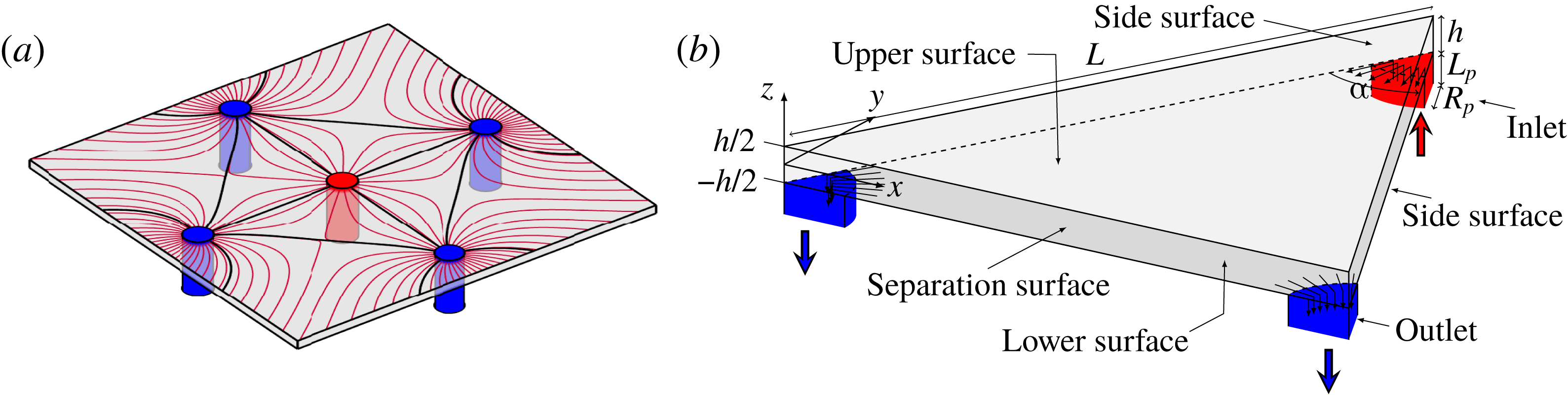
(a) Sketch showing a multipolar flow set by one inlet pipe (drawn in red) and four outlet pipes (drawn in blue) connected perpendicularly to one of two parallel plates. Separatrices (plain black lines) delineate subsets – or segments – of the flow field containing all the possible trajectories of a fluid particle released at a given inlet (see Zouache et al. (Reference Zouache, Eames, Klettner and Luthert2016) for a detailed description of the topology of the flow field). (b) Schematic of the reduced flow domain, which consists of an isosceles prism characterised by a vertex angle
 $\unicode[STIX]{x1D6FC}$
, a side length
 $L$
and a thickness
 $h$
connected to pipe inlets (drawn in red) and outlets (drawn in blue) of equal radius and length
 $R_{p}$
and
 $L_{p}$
, respectively. This reduced flow domain represents a portion of a subset of the flow field and is therefore not designed to tessellate the flow domain.
2 Mathematical model
2.1 Geometry
The multipolar geometry consists of a distribution of distinct pipes serving as either inlets or outlets connected perpendicularly to one of two thinly spaced parallel plates. The flow field generated by this distribution is decomposed into a finite number of non-communicating subsets – or segments – delineated by separation surfaces connecting two outlets to a stagnation point (figure 1
a). The shape of these subsets is determined by the distribution of inlets and outlets and their respective relative flow rates – see Zouache et al. (Reference Zouache, Eames, Klettner and Luthert2016) for a detailed description of the topology of the flow field. The flow is investigated in the basic unit of this segmentation, which consists of a triangular prism (figure 1
b) (Zouache et al.
Reference Zouache, Eames and Luthert2015). Importantly, this prism is not designed to tessellate the flow domain in its entirety; it represents an idealised portion of a subset of the flow field. For simplicity and without loss of generality, this elementary volume is an isosceles prism characterised by a thickness
 $h$
, a side length
 $L$
and an apex angle
 $\unicode[STIX]{x1D6FC}$
. Because subsets of the flow field may take a variety of shapes,
 $0<\unicode[STIX]{x1D6FC}<\unicode[STIX]{x03C0}$
. The shapes of the inlets and outlets are set to be the same, with internal radius
 $R_{p}$
and length
 $L_{p}$
. The flow at the pipe entrance is imposed and is characterised by a volumetric flow rate
 $Q$
and a kinematic viscosity
 $\unicode[STIX]{x1D708}$
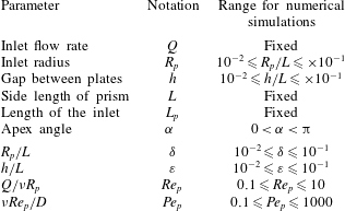
. A list of the geometrical and flow parameters present in the model is given in table 2.
2.2 Scope of calculations
List of geometrical, flow and scalar parameters and range over which they are considered in this study.
The fluid considered is incompressible and Newtonian with a dynamic viscosity
 $\unicode[STIX]{x1D707}$
and density
 $\unicode[STIX]{x1D70C}$
independent of the flow and scalar fields. This assumption is only satisfied if changes in temperature or mass within the fluid are small (Potter & Graber Reference Potter and Graber1972). The dimensionless geometrical parameters are
 $$\begin{eqnarray}\displaystyle \unicode[STIX]{x1D6FC},\quad \unicode[STIX]{x1D6FF}=\frac{R_{p}}{L},\quad \unicode[STIX]{x1D700}=\frac{h}{L},\quad l=\frac{L_{p}}{L}. & & \displaystyle\end{eqnarray}$$
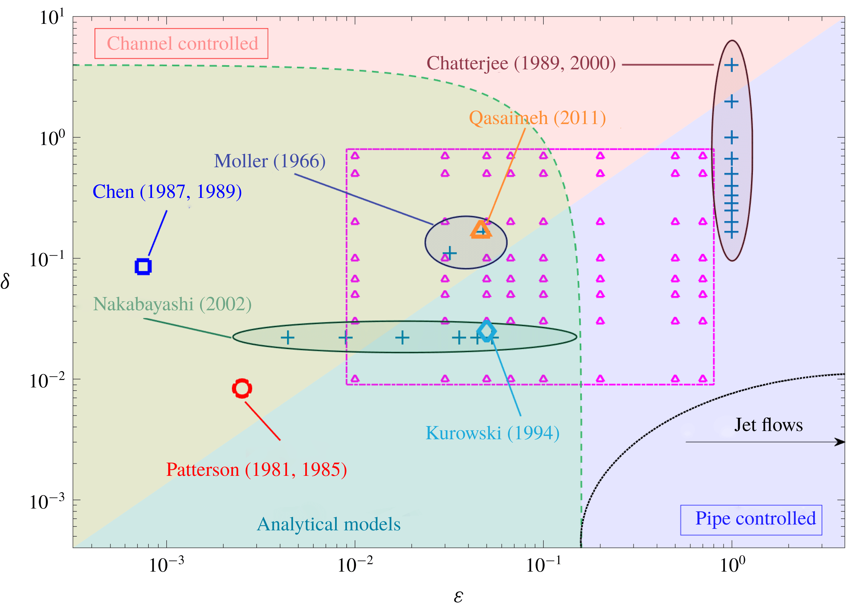
The flow and passive transport are investigated within the range of parameters
 $\unicode[STIX]{x1D6FF}$
and
 $\unicode[STIX]{x1D700}$
highlighted in figure 2, which also shows the values of these two parameters used in previous studies. The limits
 $\unicode[STIX]{x1D6FF}\ll \unicode[STIX]{x1D700}$
and
 $\unicode[STIX]{x1D700}\ll \unicode[STIX]{x1D6FF}$
correspond respectively to pipe and channel controlled flows.
Diagram showing the range of geometrical parameters
 $\unicode[STIX]{x1D6FF}$
and
 $\unicode[STIX]{x1D700}$
considered in published investigations of multipolar flows. The regions
 $\unicode[STIX]{x1D6FF}<\unicode[STIX]{x1D700}$
and
 $\unicode[STIX]{x1D700}<\unicode[STIX]{x1D6FF}$
, highlighted in the diagram in red and blue, respectively, correspond to channel and pipe controlled flows. The range of parameters for which numerical simulations were undertaken in this study with
 $Re_{p}=0.1$
, 1 and 10 are shown with
 $\triangle$
and delineated with a dotted–dashed line. The dashed line delineates the range of parameters
 $\unicode[STIX]{x1D6FF}$
and
 $\unicode[STIX]{x1D700}$
for which the analytical models developed in the present study are valid. The dotted line delineates the range of parameter values for which the inlet flow may be modelled as a jet flow.
The length of the inlet is imposed to be
 $L_{p}=0.1L$
. It is shown in § 3.2 that at very low Péclet numbers, the scalar boundary layer extends into the pipe. In this limit, the length
 $L$
is set to ensure that the full extent of upstream diffusion of disturbance in the pipe and turning regions is captured, which requires
 $L_{p}$
to be larger than the scalar boundary layer thickness. The pressure at the entrance of the pipe is uniform. It is convenient to define a Reynolds number based on the inlet flow, i.e.
 $$\begin{eqnarray}\displaystyle Re_{p}=\frac{Q}{\unicode[STIX]{x1D708}R_{p}}. & & \displaystyle\end{eqnarray}$$
Because the primary objective of the present work is to describe the fundamental characteristics of the flow and heat or mass transfers associated with the geometry of multipolar configurations, transient flow and scalar transport features are not considered. The flow and scalar field are assumed to be in a steady state, and the boundary conditions applied on the walls of the flow domain are taken to be independent of time. Transfers of the scalar are considered only at the upper plate; no-scalar flux boundary conditions are imposed on all other surfaces. The Péclet number of the flow, which describes the ratio of advective to diffusive transport, is imposed at the inlet. It is defined as
 $$\begin{eqnarray}\displaystyle Pe_{p}=\frac{Q}{DR_{p}}=\frac{\unicode[STIX]{x1D708}Re_{p}}{D}, & & \displaystyle\end{eqnarray}$$
where
 $D$
is the scalar diffusivity, which is assumed to be constant over the flow domain.
The Prandtl number (for heat transfers) – or equivalently the Schmidt number
 $Sc_{p}$
(for mass transfers) – is often used to describe passive transport. It is defined as
 $$\begin{eqnarray}\displaystyle Pr_{p}=\frac{\unicode[STIX]{x1D708}}{D}=\frac{Pe_{p}}{Re_{p}}. & & \displaystyle\end{eqnarray}$$
The Prandtl number is the ratio of diffusivity of momentum to passive material. It typically is between 0.01 and 0.03 for liquid metals, 0.7 and 1 for gases, 1 and 10 for water and 50–2000 for oils. The Schmidt number at low concentration and
 $25\,^{\circ }\text{C}$
for oxygen, hydrogen and carbon dioxide lies between 0.2 and 1 in air (
 $Pr_{p}=0.7$
) and between 100 and 500 in water (
 $Pr_{p}=7$
) (Bejan Reference Bejan2013). The flow and scalar transport are investigated over a range
 $0.1\leqslant Re_{p}\leqslant 10$
and
 $0.1\leqslant Pe_{p}\leqslant 1000$
, so that
 $0.01\leqslant Pr_{p}\leqslant 10\,000$
, which corresponds to a class of fluids ranging from gases (air) to liquids (water and oil).
2.3 Defining equations
The differential form of the conservation of mass, momentum and scalar for an incompressible Newtonian fluid with constant dynamic viscosity
 $\unicode[STIX]{x1D707}$
, density
 $\unicode[STIX]{x1D70C}$
and scalar diffusivity
 $D$
are
 $$\begin{eqnarray}\displaystyle \unicode[STIX]{x1D735}\boldsymbol{\cdot }\boldsymbol{u} & = & \displaystyle 0,\end{eqnarray}$$
 $$\begin{eqnarray}\displaystyle \unicode[STIX]{x1D70C}(\boldsymbol{u}\boldsymbol{\cdot }\unicode[STIX]{x1D735})\boldsymbol{u} & = & \displaystyle -\unicode[STIX]{x1D735}p+\unicode[STIX]{x1D735}\boldsymbol{\cdot }\unicode[STIX]{x1D749},\end{eqnarray}$$
 $$\begin{eqnarray}\displaystyle \unicode[STIX]{x1D735}\boldsymbol{\cdot }(\boldsymbol{u}C) & = & \displaystyle \unicode[STIX]{x1D735}\boldsymbol{\cdot }(D\unicode[STIX]{x1D735}C),\end{eqnarray}$$
respectively, where
 $p$
is the pressure,
 $\boldsymbol{u}$
is the velocity field and
 $\unicode[STIX]{x1D749}$
is the Newtonian viscous stress tensor.
Because of the large variations in the flow field and scalar characteristics across the flow domain, no simple and meaningful global normalisation can be found. Therefore, we decided to keep our analysis dimensional and to provide dimensionless results in specific regions of the flow domain.
2.4 Boundary conditions
The equations for the flow are solved subject to the boundary condition (see table 3)
 $$\begin{eqnarray}\displaystyle \boldsymbol{u}=2u_{p}\left(1-\left(\frac{r}{R_{p}}\right)^{2}\right)\hat{\boldsymbol{z}}, & & \displaystyle\end{eqnarray}$$
imposed at the inlet, where
 $\hat{\boldsymbol{z}}$
is the axis pointing vertical upwards and
 $u_{p}$
is the mean velocity through the pipe. The volume flux of the inlet flow is
 $$\begin{eqnarray}\displaystyle Q=2\unicode[STIX]{x03C0}\int _{0}^{R_{p}}\boldsymbol{u}\boldsymbol{\cdot }\hat{\boldsymbol{z}}r\,\text{d}r=\unicode[STIX]{x03C0}R_{p}^{2}u_{p}. & & \displaystyle\end{eqnarray}$$
The pressure at the outlets is constant, which for simplicity is taken to be zero. A no-slip boundary condition
 $\boldsymbol{u}=\mathbf{0}$
is imposed on the planes
 $z=-h/2$
and
 $z=h/2$
. Since the reduced geometry represents the elementary portion of a multipolar flow, the velocity is taken to be continuous over the sidewalls and the condition
 $$\begin{eqnarray}\displaystyle \hat{\boldsymbol{n}}\boldsymbol{\cdot }\unicode[STIX]{x1D735}\boldsymbol{u}=0, & & \displaystyle\end{eqnarray}$$
where
 $\hat{\boldsymbol{n}}$
is a unit vector perpendicular to the side wall surfaces, is applied.
A no-flux boundary condition is imposed at the side surfaces of the pipes and prism because the reduced geometry is an element of symmetry of a multipolar flow, i.e.
 $$\begin{eqnarray}\displaystyle \hat{\boldsymbol{n}}\boldsymbol{\cdot }D\unicode[STIX]{x1D735}C=0. & & \displaystyle\end{eqnarray}$$
A no-flux boundary condition is also applied to the outer surface of the pipe and to the lower plate so that transfers of the scalar occur solely through the upper plate. There are many types of boundary conditions for the scalar field that can be applied there depending on the nature of the analysis and the field of application (see Introduction). They all involve either setting the scalar, the scalar flux, or both (Shah & London Reference Shah and London1978). The two cases studied here are Dirichlet and Neumann conditions, which are
 $$\begin{eqnarray}\displaystyle C(x,y,h/2,t) & = & \displaystyle C_{1}\quad (\text{D}),\end{eqnarray}$$
 $$\begin{eqnarray}\displaystyle \hat{\boldsymbol{n}}\boldsymbol{\cdot }D\unicode[STIX]{x1D735}C & = & \displaystyle \unicode[STIX]{x1D70E}\quad (\text{N}),\end{eqnarray}$$
where
 $\unicode[STIX]{x1D70E}$
is a constant and for simplicity
 $C_{1}$
is taken to be zero. A constant and uniform scalar
 $C_{inlet}=C_{0}$
is imposed over the inlet surface, where
 $C_{0}=1$
when
 $(\text{D})$
is imposed and
 $C_{0}=0$
when
 $(\text{N})$
is applied.
List of flow and scalar boundary conditions applied to the surfaces of the flow domain.

2.5 Methods of resolution
A schematic of the computational domain is shown in figure 1(b). Axisymmetric, planar and three-dimensional simulations were undertaken and are respectively described in §§ 3, 4 and 5. Typically, more than 25 points across the thickness of the channel and the pipes were used to resolve the flow and scalar fields. The flow domain was meshed using the software Gmsh (Geuzaine & Remacle Reference Geuzaine and Remacle2009). Between 300 000 and
 $2\times 10^{6}$
nodes were used in the computations. The system of equations (2.5)–(2.7) was expressed in a finite element formulation and solved using an in-house code ‘ACEsim’ with the characteristic based split scheme (Nicolle & Eames Reference Nicolle and Eames2011; Klettner et al.
Reference Klettner, Eames, Semsarzadeh and Nicolle2016). The defining equations were solved in two steps: involving first the calculation of the velocity field until the flow field ran to steady state. The second step was to determine the scalar field for the two boundary conditions
 $(\text{D})$
and
 $(\text{N})$
.
The entrance region of the flow domain is the region with the largest changes in both velocity and scalar fields. Since the gradient of their variation is sensitive to the ratio
 $\unicode[STIX]{x1D6FF}/\unicode[STIX]{x1D700}$
and to
 $\unicode[STIX]{x1D6FC}$
, mesh independence was tested by considering the extreme cases
 $\unicode[STIX]{x1D6FF}/\unicode[STIX]{x1D700}=0.1$
and
 $\unicode[STIX]{x1D6FF}/\unicode[STIX]{x1D700}=10$
for the axisymmetric model,
 $\unicode[STIX]{x1D6FC}=\unicode[STIX]{x03C0}/12$
for the depth-averaged model and
 $\unicode[STIX]{x1D6FC}=\unicode[STIX]{x03C0}/12$
with
 $\unicode[STIX]{x1D6FF}/\unicode[STIX]{x1D700}=0.1$
and
 $\unicode[STIX]{x1D6FF}/\unicode[STIX]{x1D700}=10$
for the three-dimensional model. Numerical solutions were generated for
 $Re_{p}=1$
and
 $Pe_{p}=1000$
for both boundary conditions (
 $\text{D}$
) and (
 $\text{N}$
), and the velocity and scalar fields in the entrance region were compared with double the resolution. For all cases the flow and scalar fields agreed within 1 %.
2.6 Diagnostic tools
The flow in the prism is controlled by the pressure drop between the inlet and the outlets. Since
 $p=0$
on the outlet surface, it is defined as
 $$\begin{eqnarray}\displaystyle \unicode[STIX]{x0394}p_{t}=\frac{1}{S}\int _{\mathit{Inlet}}p\,\text{d}S, & & \displaystyle\end{eqnarray}$$
where
 $S$
is the surface area of the inlet.
When boundary condition
 $(\text{D})$
is applied, the scalar on the upper plate is known and the diffusive scalar density flux, defined as
 $$\begin{eqnarray}\displaystyle j_{d}=-D\unicode[STIX]{x1D735}C\boldsymbol{\cdot }\hat{\boldsymbol{z}}, & & \displaystyle\end{eqnarray}$$
is evaluated on the upper plate at
 $z=h/2$
. A local normalised scalar transfer coefficient is defined as
 $$\begin{eqnarray}\displaystyle \unicode[STIX]{x1D6EC}=\frac{j_{d}h}{DC_{h}}, & & \displaystyle\end{eqnarray}$$
where
 $C_{h}$
is the cross-sectionally averaged scalar.
When boundary condition
 $(\text{N})$
is applied, the diffusive scalar flux is imposed and the scalar at the upper plate, which is here denoted
 $C_{s}$
, is evaluated.
The residence time describes the time taken by an advected fluid particle to travel between two points. The residence time of a fluid particle initially located at
 $s_{0}=(x_{0},y_{0},z_{0})$
and advected by the velocity field
 $\boldsymbol{u}$
to
 $s=(x,y,z)$
is
 $$\begin{eqnarray}\displaystyle \unicode[STIX]{x0394}T(x_{0},y_{0},z_{0};x,y,z)=\int _{0}^{s}\frac{\text{d}s}{|\boldsymbol{u}|}, & & \displaystyle\end{eqnarray}$$
where
 $s$
is a distance along a path line.
3 Near-inlet axisymmetric model
The flow and scalar field are axisymmetric near the inlet as a consequence of the geometry, slip condition on the sidewalls and the axisymmetric inlet condition. In this section, the analysis is carried out within an axisymmetric frame of reference centred on the axis of the inlet. The lateral extent of the domain is taken to be equal to
 $L$
. While the inlet condition is the same as the three-dimensional model, the outlet consists of a ring on which the constant pressure
 $p=0$
is imposed.
3.1 Flow characteristics
The symmetry axis coincides with the centre of the inlet pipe and the field variables are functions of
 $z$
and the radial coordinate
 $r=\sqrt{x^{2}+y^{2}}$
. The velocity is
 $$\begin{eqnarray}\displaystyle \boldsymbol{u}=u_{r}\hat{\boldsymbol{r}}+u_{z}\hat{\boldsymbol{z}}, & & \displaystyle\end{eqnarray}$$
where
 $\hat{\boldsymbol{r}}$
and
 $\hat{\boldsymbol{z}}$
are unit vectors. The conservation of mass ensures that at a distance
 $r\geqslant R_{p}$
from the centreline, the depth-averaged streamwise velocity within the channel is
 $$\begin{eqnarray}\displaystyle u_{h}=\frac{1}{h}\int _{-h/2}^{h/2}u_{r}\,\text{d}z=\frac{Q}{2\unicode[STIX]{x03C0}rh}. & & \displaystyle\end{eqnarray}$$
By combining (2.9) and (3.2), a local Reynolds number in the channel region may be defined as
 $$\begin{eqnarray}\displaystyle Re_{c}=\frac{u_{h}h}{\unicode[STIX]{x1D708}}=Re_{p}\frac{\unicode[STIX]{x1D6FF}}{(r/L)}. & & \displaystyle\end{eqnarray}$$
Thus, the channel Reynolds number decreases with distance from the inlet pipe and has a value
 $Re_{p}O(\unicode[STIX]{x1D6FF})$
in the flow interior. This affects many aspects of the flow, including the distance from the channel entrance where the flow velocity is parabolic (see figure 3
b,c). Figure 3(a) shows the contour distribution of the radial velocity
 $u_{r}/u_{h}$
for
 $Re_{p}=1$
,
 $\unicode[STIX]{x1D6FF}=0.05$
and
 $\unicode[STIX]{x1D700}=0.01$
, 0.05 and 0.1. For low Reynolds number, the flow adjusts over a distance
 $O(h)$
so that it is expected to be parabolic over most of the channel length.
(a) Contour distributions of the radial velocity field
 $u_{r}/u_{h}$
are shown for fixed
 $Re_{p}=1$
,
 $\unicode[STIX]{x1D6FF}=0.05$
and
 $\unicode[STIX]{x1D700}=0.01$
, 0.05 and 0.1. (b,c) Variations of the velocity profile
 $u_{r}/u_{h}$
across a channel cross-section plotted at various distances from the inlet centreline (colour-coded in a) are shown for (b)
 $\unicode[STIX]{x1D700}=0.1$
and (c)
 $\unicode[STIX]{x1D700}=0.01$
. The analytical parabolic profile (3.5b,c
) is shown with
 $+$
.

(a) Contour distributions of the pressure field
 $p/\unicode[STIX]{x0394}p_{t}$
are shown for fixed
 $Re_{p}=1$
,
 $\unicode[STIX]{x1D6FF}=0.05$
and
 $\unicode[STIX]{x1D700}=0.01$
, 0.05 and 0.1. (b) Variations of the pressure
 $p_{c}/\unicode[STIX]{x0394}p_{c}$
across the upper plate are shown on a linear scale and (inset) a logarithmic scale for fixed
 $Re_{p}=1$
,
 $\unicode[STIX]{x1D6FF}=0.05$
and
 $\unicode[STIX]{x1D700}=0.01$
, 0.02, 0.05, 0.067 and 0.1. The analytical solution (3.6) is plotted with
 $+$
. (c) Variation of the dimensionless pressure drop
 $\unicode[STIX]{x03C0}L^{3}\unicode[STIX]{x0394}p_{t}/2\unicode[STIX]{x1D707}Q$
with
 $\unicode[STIX]{x1D6FF}/\unicode[STIX]{x1D700}$
calculated analytically (3.9) (plain lines) and numerically for
 $Re_{p}=0.1$
, 1 and 10.

When
 $\unicode[STIX]{x1D700}\ll 1$
, a lubrication approximation (Reynolds (Reference Reynolds1886), Section IV, equation (12)) may be applied to simplify the radial momentum equation. By denoting
 $p_{c}$
the pressure in the channel, the radial velocity may then be expressed as (Pinkus & Sternlicht Reference Pinkus and Sternlicht1961)
 $$\begin{eqnarray}\displaystyle u_{r}=u_{h}{\mathcal{F}}_{u}({\check{z}}), & & \displaystyle\end{eqnarray}$$
where
 $$\begin{eqnarray}\displaystyle u_{h}=-\frac{h^{2}}{12\unicode[STIX]{x1D707}}\frac{\text{d}p_{c}}{\text{d}r},\quad {\mathcal{F}}_{u}({\check{z}})=\frac{3}{2}(1-{\check{z}}^{2}),\quad {\check{z}}=\frac{2z}{h}. & & \displaystyle\end{eqnarray}$$
Integrating (3.5) and setting the outlet pressure to be zero retrieves the relationship
 $$\begin{eqnarray}\displaystyle p_{c}(r)=-\frac{6Q\unicode[STIX]{x1D707}}{\unicode[STIX]{x03C0}h^{3}}\log \left(\frac{r}{L}\right), & & \displaystyle\end{eqnarray}$$
derived by Livesey (Reference Livesey1960) (equation (8)). The pressure drop across the channel region is then
 $$\begin{eqnarray}\displaystyle \unicode[STIX]{x0394}p_{c}=p_{c}(R_{p})=-\frac{6Q\unicode[STIX]{x1D707}}{\unicode[STIX]{x03C0}h^{3}}\log \unicode[STIX]{x1D6FF}. & & \displaystyle\end{eqnarray}$$
Numerical solutions, plotted in figure 4(b) for
 $Re_{p}=1$
,
 $\unicode[STIX]{x1D6FF}=0.05$
and varying channel aspect ratios
 $\unicode[STIX]{x1D700}$
, show good agreement with (3.6). For a long inlet pipe, where the parabolic profile (2.8) extends over a large fraction of its length
 $L_{p}$
, the pressure drop across the pipe length
 $\unicode[STIX]{x0394}p_{p}$
is estimated to be (Batchelor Reference Batchelor1957)
 $$\begin{eqnarray}\displaystyle \unicode[STIX]{x0394}p_{p}=\frac{8\unicode[STIX]{x1D707}L_{p}Q}{\unicode[STIX]{x03C0}R_{p}^{4}}. & & \displaystyle\end{eqnarray}$$
A semi-empirical approach to estimate the pressure drop
 $\unicode[STIX]{x0394}p_{t}$
over the totality of the flow domain is obtained by adding (3.7) and (3.8)
 $\unicode[STIX]{x0394}p_{t}\simeq \unicode[STIX]{x0394}p_{c}+\unicode[STIX]{x0394}p_{p}$
, where
 $$\begin{eqnarray}\displaystyle \frac{\unicode[STIX]{x03C0}L^{3}\unicode[STIX]{x0394}p_{t}}{2\unicode[STIX]{x1D707}Q}=\frac{4l}{\unicode[STIX]{x1D6FF}^{4}}-\frac{3}{\unicode[STIX]{x1D700}^{3}}\log \unicode[STIX]{x1D6FF}. & & \displaystyle\end{eqnarray}$$
This relation describes the interdependence between the two geometrical parameters
 $\unicode[STIX]{x1D6FF}$
and
 $\unicode[STIX]{x1D700}$
in setting the total pressure drop. It agrees with numerical calculations over the range of parameters considered, as shown in figure 4(c). When
 $\unicode[STIX]{x1D700}\ll \unicode[STIX]{x1D6FF}$
, the pressure drop is controlled by the channel region; whereas when
 $\unicode[STIX]{x1D6FF}\ll \unicode[STIX]{x1D700}$
it is controlled by the inlet pipe. This is well illustrated in figure 4(a), which shows contour distributions of the pressure field normalised by the pressure drop for
 $Re_{p}=1$
,
 $\unicode[STIX]{x1D6FF}=0.05$
and varying channel aspect ratios
 $\unicode[STIX]{x1D700}$
.
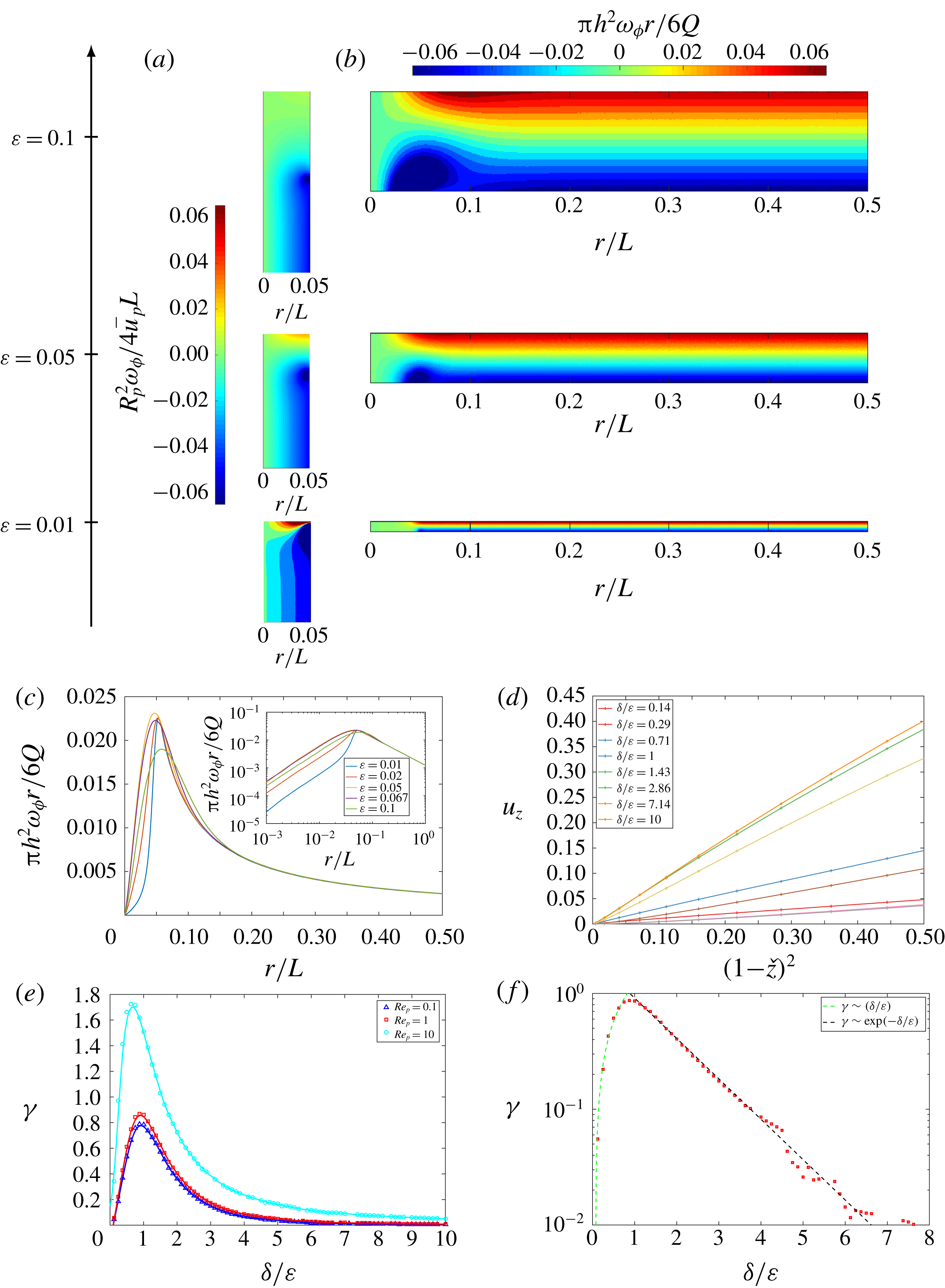
(a,b) Contour distributions of the vorticity field (a)
 $R_{p}^{2}\unicode[STIX]{x1D714}_{\unicode[STIX]{x1D719}}/4u_{p}L$
in the pipe region and (b)
 $\unicode[STIX]{x03C0}h^{2}\unicode[STIX]{x1D714}_{\unicode[STIX]{x1D719}}r/6Q$
in the channel region are shown for
 $Re_{p}=1$
,
 $\unicode[STIX]{x1D6FF}=0.05$
and
 $\unicode[STIX]{x1D700}=0.01$
, 0.05 and 0.1. (c) Variation of the vorticity at the upper plate
 $\unicode[STIX]{x03C0}h^{2}\unicode[STIX]{x1D714}_{\unicode[STIX]{x1D719}}r/6Q$
with distance from the inlet centreline for fixed
 $Re_{p}=1$
,
 $\unicode[STIX]{x1D6FF}=0.05$
and varying channel aspect ratios
 $\unicode[STIX]{x1D700}=0.01$
, 0.02, 0.05, 0.067 and 0.1. (d) Variations of the vertical velocity along the centreline
 $u_{z}$
with
 $(1-{\check{z}}^{2})$
shown for fixed
 $Re_{p}=1$
and various
 $\unicode[STIX]{x1D6FF}/\unicode[STIX]{x1D700}$
. (e,f) Variations of the strain rate
 $\unicode[STIX]{x1D6FE}$
with
 $\unicode[STIX]{x1D6FF}/\unicode[STIX]{x1D700}$
are plotted for (e)
 $Re_{p}=0.1$
, 1 and 10 on a linear scale and (f)
 $Re_{p}=1$
on a semi-logarithmic scale. The plain lines correspond to cubic spline interpolants.
The above analysis provides some understanding and appreciation of the flow and pressure field within the pipe and channel regions. It is based heavily on having a physical dimension much smaller than a distance, which in turn depends on either
 $\unicode[STIX]{x1D6FF}$
,
 $\unicode[STIX]{x1D700}$
or both being small. The turning region is complex but there are some important observations, particularly at the stagnation point that sits opposite the pipe. The azimuthal vorticity is
 $$\begin{eqnarray}\displaystyle \unicode[STIX]{x1D714}_{\unicode[STIX]{x1D719}}\left(=\frac{\unicode[STIX]{x2202}u_{r}}{\unicode[STIX]{x2202}z}-\frac{\unicode[STIX]{x2202}u_{z}}{\unicode[STIX]{x2202}r}\right)=\frac{4u_{p}r}{R_{p}^{2}}, & & \displaystyle\end{eqnarray}$$
within the pipe. Within the channel, positive and negative vorticities of equal strength are generated on the top and bottom walls as a consequence of the no-slip condition (see figure 5
b). The cross-stream diffusion leads to vorticity cancellation and a linear variation of
 $\unicode[STIX]{x1D714}_{\unicode[STIX]{x1D719}}$
across the channel, resulting in
 $$\begin{eqnarray}\displaystyle \unicode[STIX]{x1D714}_{\unicode[STIX]{x1D719}}=\frac{6Qz}{\unicode[STIX]{x03C0}h^{3}r}, & & \displaystyle\end{eqnarray}$$
(see figure 5 c).
The flow in the turning region is dominated by strain which extends quite far into the pipe region. At the upper plate, the flow is approximately an axisymmetric stagnation point flow. The nature of the strain is determined by the ratio between the inlet radius and the channel aspect ratio
 $\unicode[STIX]{x1D6FF}/\unicode[STIX]{x1D700}$
. For wide channels (
 $\unicode[STIX]{x1D700}\geqslant \unicode[STIX]{x1D6FF}$
) the stagnation flow is largely irrotational, while for
 $\unicode[STIX]{x1D700}\ll \unicode[STIX]{x1D6FF}$
the stagnation flow is largely viscously dominated. In the vicinity of the wall (as
 $z\rightarrow h/2$
),
 $u_{z}\rightarrow 0$
and
 $u_{r}\rightarrow 0$
. The flow in the vicinity of the stagnation point can be expanded as a Taylor series in
 $z$
and
 $r$
. Assuming that the leading-order flow can be described as the first term in the series, an approximate power-law model of the stagnation flow that satisfies mass conservation can be introduced, i.e.
 $$\begin{eqnarray}\displaystyle u_{r}=\frac{\unicode[STIX]{x1D6FE}}{m}\left(z-\frac{h}{2}\right)^{n}r^{m},\quad u_{z}=\frac{\unicode[STIX]{x1D6FE}}{n}\left(z-\frac{h}{2}\right)^{n+1}r^{m-1}, & & \displaystyle\end{eqnarray}$$
where
 $n$
and
 $m$
are constants. For
 $u_{z}$
to be bounded at
 $r=0$
,
 $m\geqslant 1$
; likewise for the no-slip condition to be satisfied at
 $z=h/2$
,
 $n>0$
. The smallest integers that describe the viscous straining flow are
 $m=1$
,
 $n=1$
, when
 $\unicode[STIX]{x1D6FE}$
has dimensions
 $[L^{-1}][T^{-1}]$
. This model agrees with the numerical solution, as illustrated in figure 5(d), which shows the variation of
 $u_{z}$
along the inlet centreline as a function of
 $(1-{\check{z}})^{2}$
for various
 $\unicode[STIX]{x1D6FF}/\unicode[STIX]{x1D700}$
. The value of
 $\unicode[STIX]{x1D6FE}$
was calculated numerically for
 $0.1\leqslant \unicode[STIX]{x1D6FF}/\unicode[STIX]{x1D700}\leqslant 10$
and
 $Re_{p}=0.1$
, 1 and 10, and a best fit was determined for both
 $\unicode[STIX]{x1D6FF}\ll \unicode[STIX]{x1D700}$
and
 $\unicode[STIX]{x1D6FF}\geqslant \unicode[STIX]{x1D700}$
. For
 $\unicode[STIX]{x1D6FF}\ll \unicode[STIX]{x1D700}$
,
 $\unicode[STIX]{x1D6FE}$
varies approximately linearly with
 $\unicode[STIX]{x1D6FF}/\unicode[STIX]{x1D700}$
. For
 $\unicode[STIX]{x1D6FF}\geqslant \unicode[STIX]{x1D700}$
, the strain rate varies approximately as an inverse exponential of
 $\unicode[STIX]{x1D6FF}/\unicode[STIX]{x1D700}$
(see figure 5
e,f).
3.2 Scalar field with boundary condition (
 $\mathit{D}$
)

The characteristics of the transport of the scalar are determined by the Péclet number, or specifically the thickness of the scalar boundary layer as compared to the velocity boundary layer. For thin scalar boundary layers,
 $$\begin{eqnarray}\displaystyle D\ll h\unicode[STIX]{x1D6FE}=u_{p}/R_{p}, & & \displaystyle\end{eqnarray}$$
so that
 $Pe_{p}\gg 1$
. For
 $Pe_{p}\ll 1$
, the diffusive boundary layer extends into the pipe so that transfers occur solely in the turning region. While the differential form of the conservation law (2.7) is ultimately what is solved numerically, its integral form, which is
 $$\begin{eqnarray}\displaystyle \frac{1}{r}\frac{\text{d}}{\text{d}r}\left(r\int _{\unicode[STIX]{x1D701}}^{h/2}u_{r}C\,\text{d}z\right)=D\left(\frac{1}{r}\frac{\text{d}}{\text{d}r}\left(r\frac{\text{d}}{\text{d}r}\left(\int _{\unicode[STIX]{x1D701}}^{h/2}C\,\text{d}z\right)\right)+\left[\frac{\unicode[STIX]{x2202}C}{\unicode[STIX]{x2202}z}\right]_{z=h/2}\right), & & \displaystyle\end{eqnarray}$$
will also be considered. The limit
 $\unicode[STIX]{x1D701}$
depends on the region where the integral is taken, for instance
 $\unicode[STIX]{x1D701}\rightarrow -\infty$
for the turning region and
 $\unicode[STIX]{x1D701}=-h/2$
for the channel region. An advantage of the integral form of the conservation law is that contrary to the differential form, it explicitly includes the boundary conditions.
3.2.1 Turning region
Close to the wall (
 $r\ll 1$
), transport is dominated by vertical diffusion, reducing (2.7) to
 $$\begin{eqnarray}\displaystyle u_{z}\frac{\unicode[STIX]{x2202}C}{\unicode[STIX]{x2202}z}\simeq D\frac{\unicode[STIX]{x2202}^{2}C}{\unicode[STIX]{x2202}z^{2}}. & & \displaystyle\end{eqnarray}$$
Within the turning region, the boundary layer straining flow is described by (3.12). A similarity solution of the form
 $C(r,z)={\mathcal{C}}(r){\mathcal{G}}(\unicode[STIX]{x1D702})$
, where
 $\unicode[STIX]{x1D702}=(h/2-z)/\unicode[STIX]{x1D6FF}_{t}(r)$
and
 $\unicode[STIX]{x1D6FF}_{t}$
is the scalar boundary layer thickness, that satisfies
 $C(r,\unicode[STIX]{x1D702}=0)=0$
and
 $C(r,\unicode[STIX]{x1D702}\rightarrow -\infty )=1$
is sought. One such solution is easily identified (Acrivos Reference Acrivos1962), i.e.
 $$\begin{eqnarray}\displaystyle C(r,z)=\frac{3^{2/3}}{\unicode[STIX]{x0393}(1/3)}\int _{0}^{(h/2-z)/(D/\unicode[STIX]{x1D6FE})^{1/3}}\exp \left(-\frac{\unicode[STIX]{x1D709}^{3}}{3}\right)\text{d}\unicode[STIX]{x1D709}, & & \displaystyle\end{eqnarray}$$
where
 $\unicode[STIX]{x0393}$
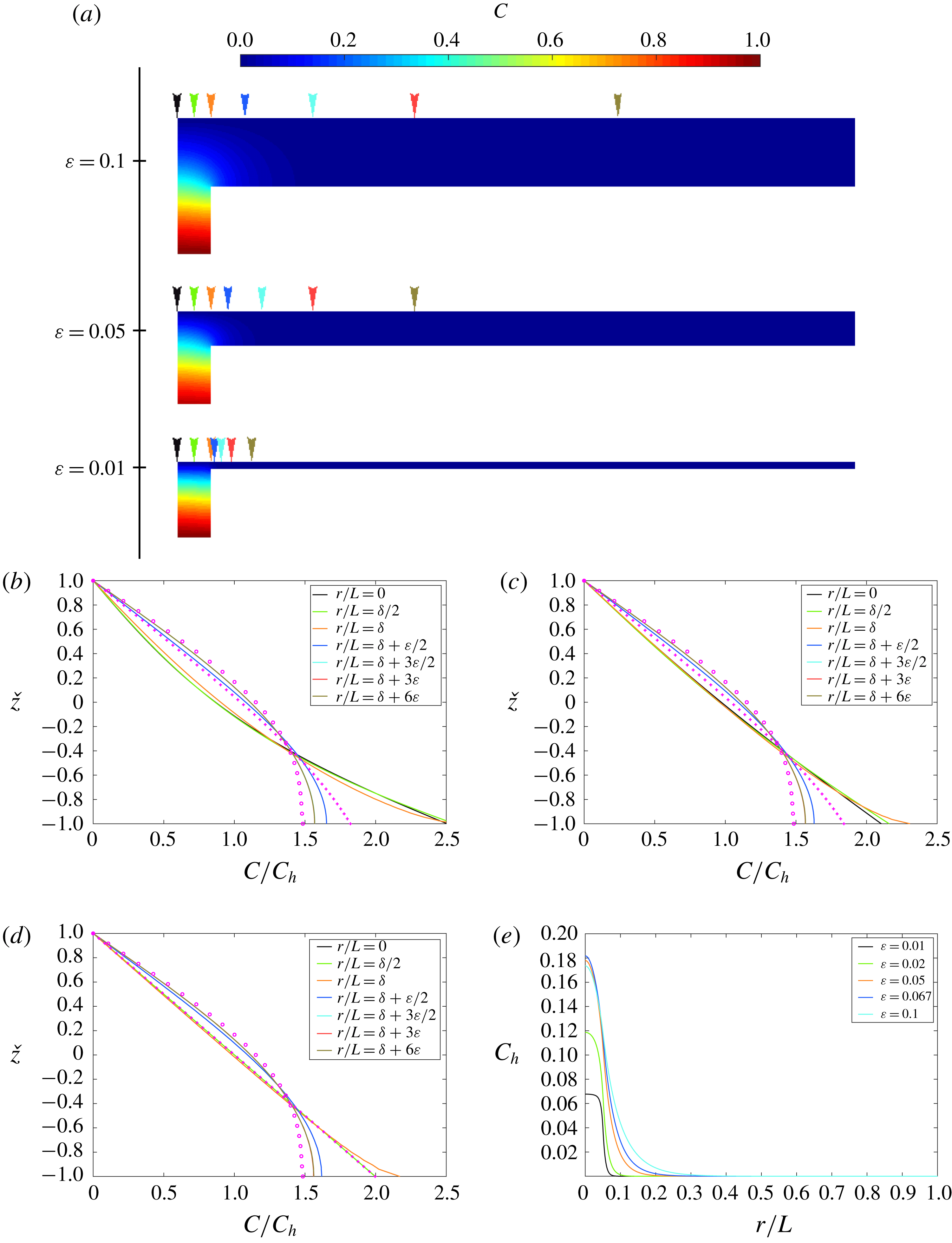
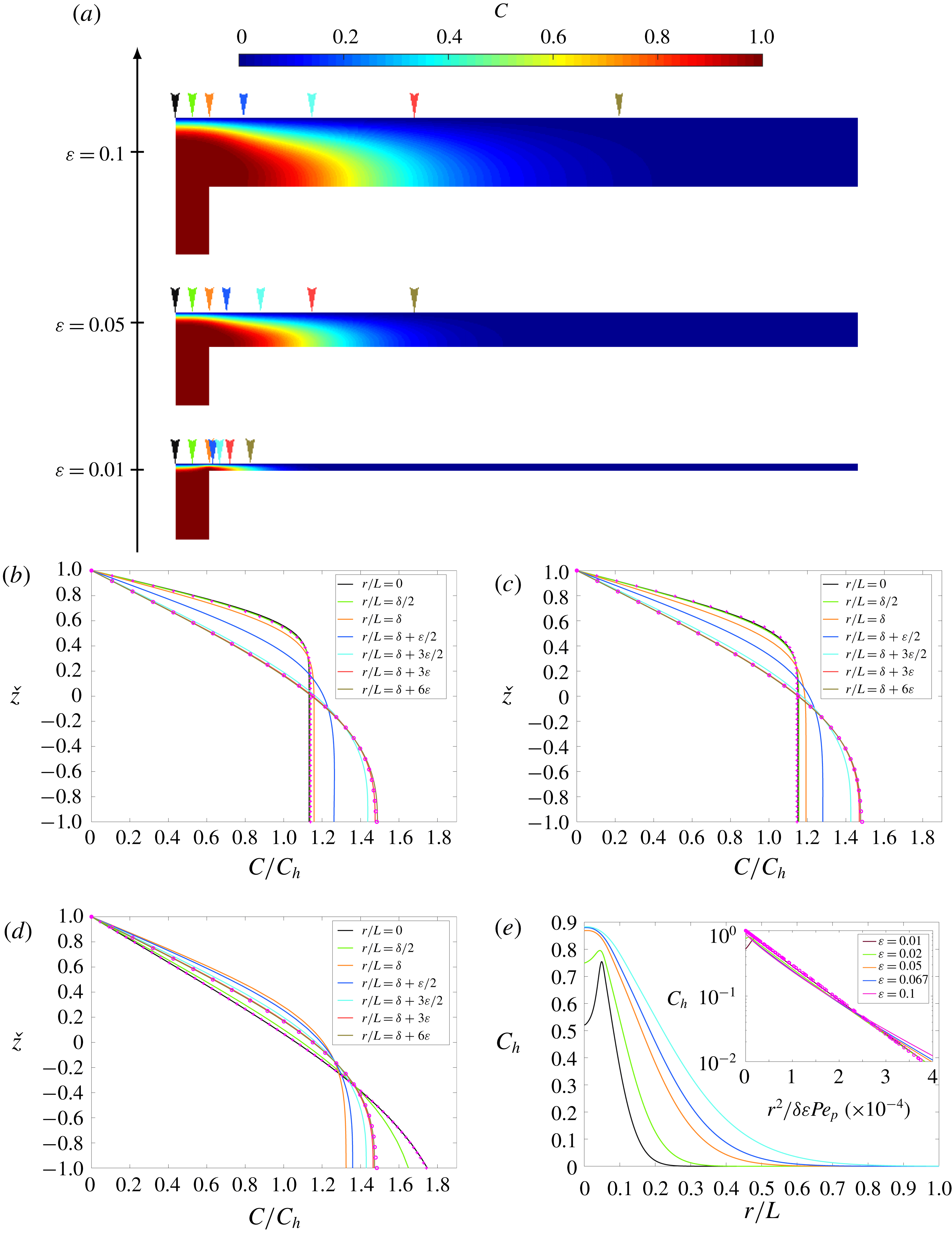
is the Euler gamma function (Abramowitz & Stegun Reference Abramowitz and Stegun1972). Scalar contour distributions and scalar profiles across the turning region calculated analytically and numerically are shown in figures 6 and 7 for
 $\unicode[STIX]{x1D6FF}=0.05$
, various channel aspect ratios,
 $Re_{p}=1$
and
 $Pe_{p}=1$
and 100, respectively. The profiles in the region
 $0\leqslant r/L<\unicode[STIX]{x1D6FF}$
collapse onto the same curve and are therefore independent of the radial coordinate. The scalar flux through the upper plate is
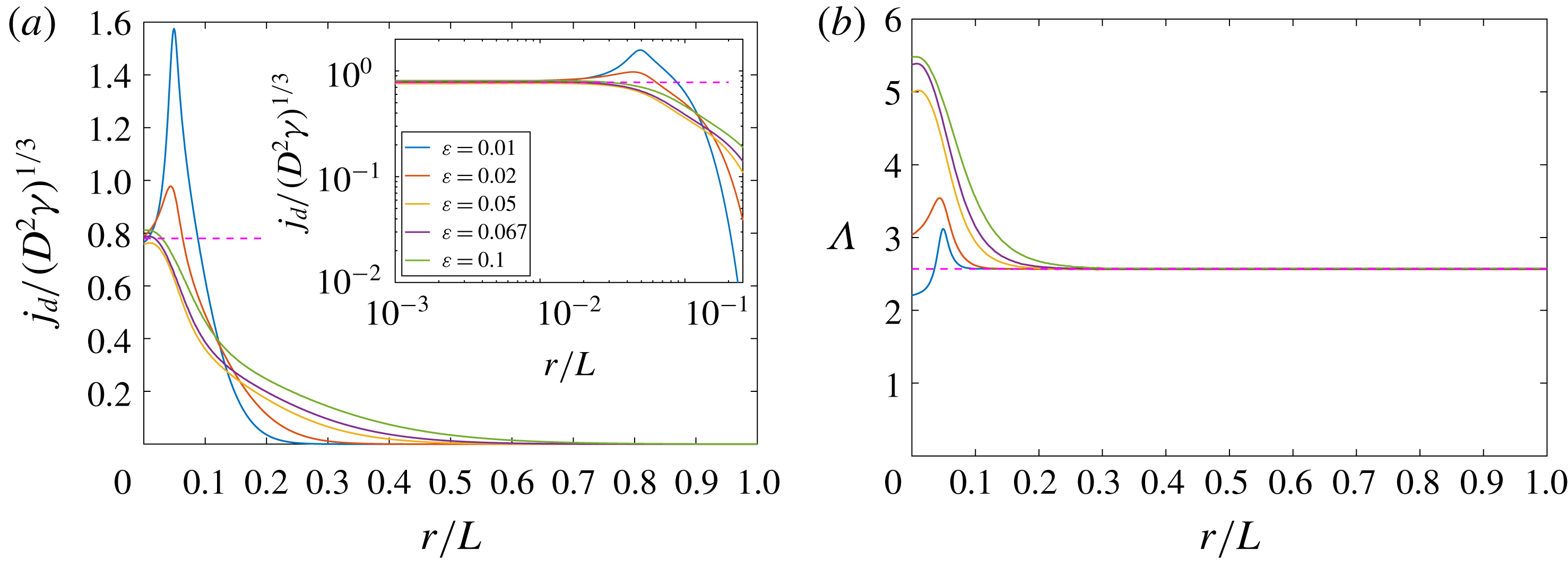
 $$\begin{eqnarray}\displaystyle j_{d}=\frac{3^{2/3}}{\unicode[STIX]{x0393}(1/3)}(D^{2}\unicode[STIX]{x1D6FE})^{1/3}\simeq 0.78(D^{2}\unicode[STIX]{x1D6FE})^{1/3}. & & \displaystyle\end{eqnarray}$$
The variation of
 $j_{d}$
with distance from the inlet centreline is plotted later in figure 9(a) for
 $\unicode[STIX]{x1D6FF}=0.05$
,
 $Re_{p}=1$
,
 $Pe_{p}=100$
and various channel aspect ratios. The figure shows that
 $j_{d}$
is independent of the radial distance from the stagnation point and that it remains constant for
 $0\leqslant r/L<\unicode[STIX]{x1D6FF}$
.
(Boundary condition
 $\text{D}$
) (a) Contour distributions of the scalar field
 $C$
are shown for
 $Re_{p}=1$
,
 $Pe_{p}=1$
,
 $\unicode[STIX]{x1D6FF}=0.05$
and
 $\unicode[STIX]{x1D700}=0.01$
, 0.05 and 0.1. (b,c,d) Variation of the scalar
 $C/C_{h}$
across a channel cross-section for
 $Re_{p}=1$
,
 $Pe_{p}=1$
,
 $\unicode[STIX]{x1D6FF}=0.05$
and (b)
 $\unicode[STIX]{x1D700}=0.1$
, (c)
 $\unicode[STIX]{x1D700}=0.05$
and (d)
 $\unicode[STIX]{x1D700}=0.01$
plotted at various distances from the inlet centreline (colour-coded in a). The analytical solutions in the entrance region (3.16) (
 $+$
) and channel region (3.26) (
 $\circ$
) are also shown. (e) Variation of the cross-sectionally averaged scalar
 $C_{h}$
with distance from the inlet centreline for
 $Re_{p}=1$
,
 $Pe_{p}=1$
,
 $\unicode[STIX]{x1D6FF}=0.05$
and
 $\unicode[STIX]{x1D700}=0.01$
, 0.02, 0.05, 0.067 and 0.1.
(Boundary condition
 $\text{D}$
) (a) Contour distributions of the scalar field
 $C$
are shown for
 $Re_{p}=1$
,
 $Pe_{p}=100$
,
 $\unicode[STIX]{x1D6FF}=0.05$
and
 $\unicode[STIX]{x1D700}=0.01$
, 0.05 and 0.1. (b,c,d) Variation of the scalar
 $C/C_{h}$
across a channel cross-section for
 $Re_{p}=1$
,
 $Pe_{p}=100$
,
 $\unicode[STIX]{x1D6FF}=0.05$
and (b)
 $\unicode[STIX]{x1D700}=0.1$
, (c)
 $\unicode[STIX]{x1D700}=0.05$
and (d)
 $\unicode[STIX]{x1D700}=0.01$
plotted at various distances from the inlet centreline (colour-coded in a). The analytical solutions in the entrance region (3.16) (
 $+$
) and channel region (3.26) (
 $\circ$
) are also shown. (e) Variation of the cross-sectionally averaged scalar
 $C_{h}$
with
 $r^{2}/\unicode[STIX]{x1D6FF}\unicode[STIX]{x1D700}Pe_{p}$
for
 $Re_{p}=1$
,
 $Pe=100$
,
 $\unicode[STIX]{x1D6FF}=0.05$
and
 $\unicode[STIX]{x1D700}=0.01$
, 0.02, 0.05, 0.067 and 0.1 are shown on a linear and in the inset on a semi-logarithmic scale. The analytical solution (3.25) is shown with
 $\circ$
.
Integral techniques have traditionally been applied to describe boundary layer development starting with Prandtl and others (Prandtl Reference Prandtl1904; von Kármán Reference von Kármán1921; Pohlhausen Reference Pohlhausen1921). Here we adapt these techniques to determine the variation of the scalar and scalar density flux. As with boundary layer flows, equation (3.14) is written in term of
 $(1-C)$
so that the integral of the advective flux is finite. In the near wall region a scalar field that satisfies the surface boundary conditions and interior conditions is defined and has the form
 $$\begin{eqnarray}\displaystyle C(r,z)=\left\{\begin{array}{@{}ll@{}}1, & \displaystyle \frac{h}{2}-\unicode[STIX]{x1D6FF}_{t}<z<\frac{h}{2}\\ \displaystyle {\mathcal{F}}_{c}\left(\frac{h/2-z}{\unicode[STIX]{x1D6FF}_{t}}\right), & \displaystyle z<\frac{h}{2}-\unicode[STIX]{x1D6FF}_{t},\end{array}\right. & & \displaystyle\end{eqnarray}$$
where
 $\unicode[STIX]{x1D6FF}_{t}$
is the scalar boundary layer thickness and is a function of
 $r$
and
 ${\mathcal{F}}_{c}$
is the constructed scalar profile, which satisfies
 $$\begin{eqnarray}\displaystyle {\mathcal{F}}_{c}(0)=0,\quad {\mathcal{F}}_{c}(1)=1. & & \displaystyle\end{eqnarray}$$
The integral expressions, in dimensionless form, can be cast as
 $$\begin{eqnarray}\displaystyle \unicode[STIX]{x1D706}_{1}=-\frac{1}{\unicode[STIX]{x1D6FF}_{t}^{2}}\int _{-\infty }^{h/2}\!\left(z-\frac{h}{2}\right)\!(1-C)\text{d}z,\quad \unicode[STIX]{x1D706}_{2}=\frac{1}{\unicode[STIX]{x1D6FF}_{t}}\int _{-\infty }^{h/2}\!(1-C)\,\text{d}z,\quad \unicode[STIX]{x1D706}_{3}=-\unicode[STIX]{x1D6FF}_{t}\left[\frac{\unicode[STIX]{x2202}C}{\unicode[STIX]{x2202}z}\right]_{z=h/2}. & & \displaystyle \nonumber\\ \displaystyle & & \displaystyle\end{eqnarray}$$
The first term
 $\unicode[STIX]{x1D706}_{1}$
includes the shear in the radial velocity which gives rise to a non-Fickian transport. Integral techniques have the advantage that all the terms in (3.14) are retained, although they require an approximate form of the scalar profile to be defined. By denoting
 $$\begin{eqnarray}\displaystyle \unicode[STIX]{x1D6FF}_{0}=\left(\frac{\unicode[STIX]{x1D706}_{3}}{2\unicode[STIX]{x1D706}_{1}}\right)^{1/3}\left(\frac{D}{\unicode[STIX]{x1D6FE}}\right)^{1/3},\quad \hat{r}=\frac{r}{\unicode[STIX]{x1D6FF}_{0}},\quad \hat{\unicode[STIX]{x1D6FF}}=\frac{\unicode[STIX]{x1D6FF}_{t}}{\unicode[STIX]{x1D6FF}_{0}}, & & \displaystyle\end{eqnarray}$$
where
 $\unicode[STIX]{x1D6FF}_{0}$
is the boundary layer thickness at
 $r=0$
, the evolution of the scalar boundary layer thickness is described by
 $$\begin{eqnarray}\displaystyle \frac{\text{d}^{2}\hat{\unicode[STIX]{x1D6FF}}}{\text{d}\hat{r}^{2}}+\left(\frac{1}{\hat{r}}+\frac{\unicode[STIX]{x1D706}_{3}}{\unicode[STIX]{x1D706}_{2}}\hat{r}\hat{\unicode[STIX]{x1D6FF}}\right)\frac{\text{d}\hat{\unicode[STIX]{x1D6FF}}}{\text{d}r}-\left(\frac{\unicode[STIX]{x1D706}_{3}}{\unicode[STIX]{x1D706}_{2}\hat{\unicode[STIX]{x1D6FF}}}-\hat{\unicode[STIX]{x1D6FF}}^{2}\right)=0. & & \displaystyle\end{eqnarray}$$
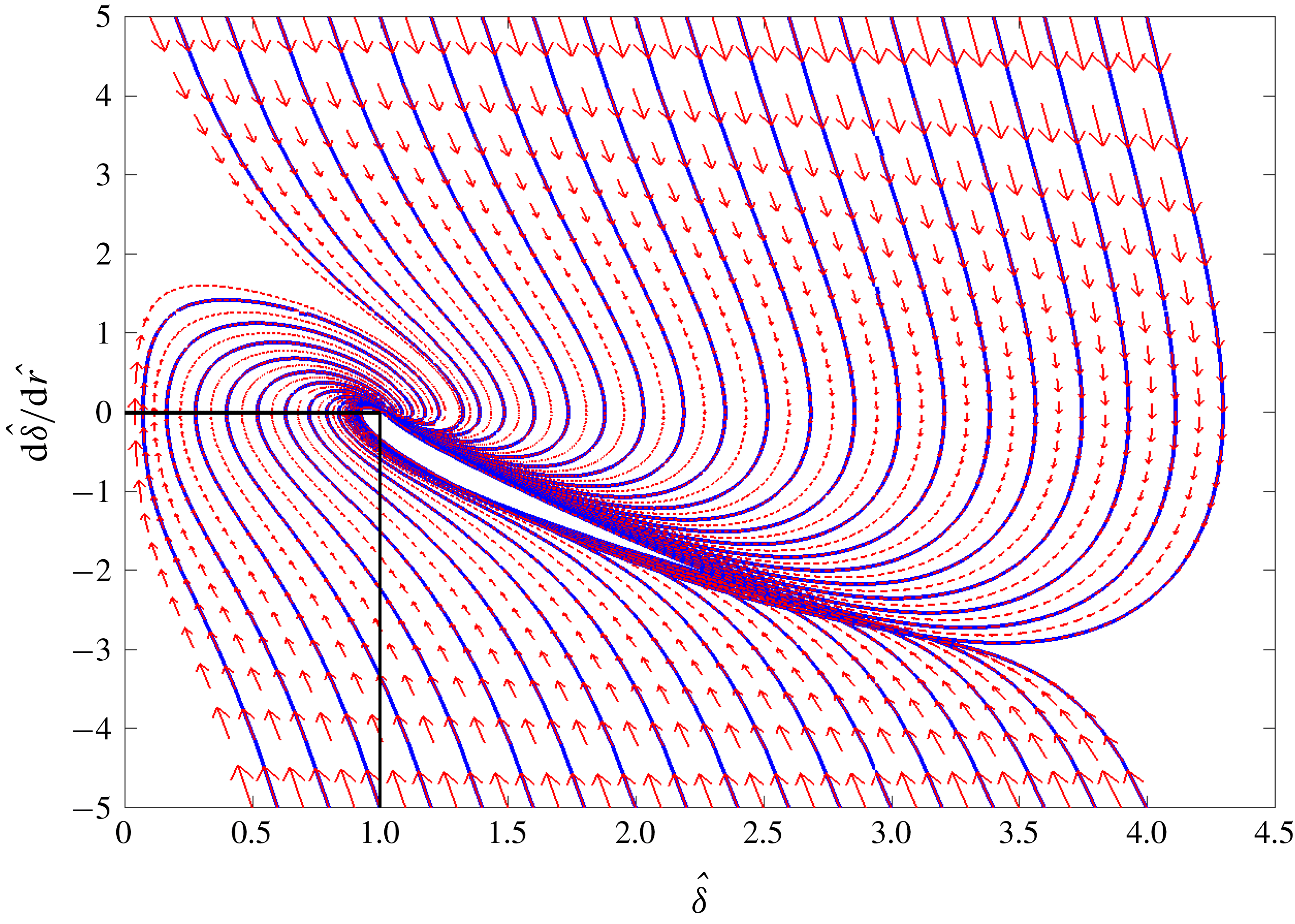
The constant scalar boundary layer thickness is due to a balance of vertical advection and vertical diffusion. If the scalar boundary layer thickness is thinner than
 $\unicode[STIX]{x1D6FF}_{0}$
, then diffusion is enhanced and the thickness grows to
 $\unicode[STIX]{x1D6FF}_{0}$
. This is shown in the phase portrait
 $(\hat{\unicode[STIX]{x1D6FF}},\text{d}\hat{\unicode[STIX]{x1D6FF}}/\text{d}\hat{r})$
plotted in figure 8 for values of
 $\unicode[STIX]{x1D706}_{2}$
and
 $\unicode[STIX]{x1D706}_{3}$
calculated from the similarity solution. This broadly explains why the scalar boundary layer thickness tends to
 $\unicode[STIX]{x1D6FF}_{t}=\unicode[STIX]{x1D6FF}_{0}$
.
Phase portrait for (3.22) showing the convergence of the scalar boundary layer thickness in the turning region to its value at the stagnation point (
 $\hat{\unicode[STIX]{x1D6FF}}=1$
). The values of
 $\unicode[STIX]{x1D706}_{2}$
and
 $\unicode[STIX]{x1D706}_{3}$
were calculated from the similarity solution (3.16).
(Boundary condition
 $\text{D}$
) Variation of (a) the diffusive flux
 $j_{d}$
in the turning region normalised by
 $(D^{2}\unicode[STIX]{x1D6FE})^{1/3}$
shown on a linear and logarithmic scale and (b) the scalar transfer coefficient
 $\unicode[STIX]{x1D6EC}$
in the channel region for
 $Re_{p}=1$
,
 $Pe_{p}=100$
,
 $\unicode[STIX]{x1D6FF}=0.05$
and varying channel aspect ratios
 $\unicode[STIX]{x1D700}=0.01$
, 0.02, 0.05, 0.067 and 0.1. The analytical solutions (3.23) and (3.28) are plotted as dashed lines.
The scalar density flux at the stagnation point is
 $$\begin{eqnarray}\displaystyle j_{d}=(2\unicode[STIX]{x1D706}_{3}^{2}\unicode[STIX]{x1D706}_{1})^{1/3}(D^{2}\unicode[STIX]{x1D6FE})^{1/3}. & & \displaystyle\end{eqnarray}$$
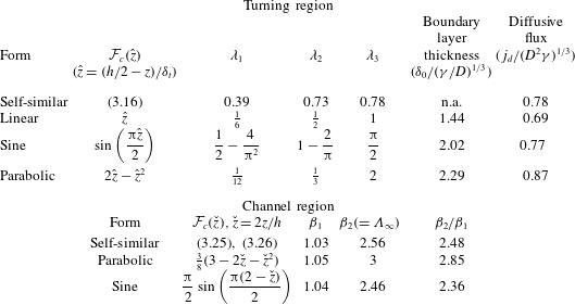
The value of the coefficients
 $\unicode[STIX]{x1D706}_{1}$
,
 $\unicode[STIX]{x1D706}_{2}$
,
 $\unicode[STIX]{x1D706}_{3}$
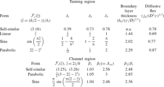
and the scalar density flux across the upper plate are given in table 4 for different constructed scalar profiles. The linear profile is the least justified because its gradient is not continuous; the value of the normalised scalar flux varies by about 12 % from the similarity solution. The sinusoidal profile gives the best approximation for the diffusive flux with a 0.01 % variation from the similarity solution.

3.2.2 Channel region
Similar approaches may be applied to determine the evolution of the scalar and scalar density flux far from the inlet centreline. By neglecting radial diffusion, equation (2.7) may be written as
 $$\begin{eqnarray}\displaystyle \frac{3Q}{4\unicode[STIX]{x03C0}rh}\left(1-\frac{4z^{2}}{h^{2}}\right)\frac{\unicode[STIX]{x2202}C}{\unicode[STIX]{x2202}r}=D\frac{\unicode[STIX]{x2202}^{2}C}{\unicode[STIX]{x2202}z^{2}}. & & \displaystyle\end{eqnarray}$$
A separable multiplicative solution of the form
 $C(r,z)=R(r)Z(z)$
is sought. From (3.24),
 $$\begin{eqnarray}\displaystyle & \displaystyle R(r)=a_{0}\exp \left(b\frac{2\unicode[STIX]{x03C0}D}{3Qh}r^{2}\right)=\exp \left(\frac{4b}{3\unicode[STIX]{x1D6FF}\unicode[STIX]{x1D700}Pe_{p}}\left(\left(\frac{r}{L}\right)^{2}-\unicode[STIX]{x1D6FF}^{2}\right)\right), & \displaystyle\end{eqnarray}$$
 $$\begin{eqnarray}\displaystyle & \displaystyle \frac{\text{d}^{2}Z}{\text{d}z^{2}}-\frac{b}{h^{2}}\left(1-\frac{4z^{2}}{h^{2}}\right)Z=0, & \displaystyle\end{eqnarray}$$
where
 $b$
is an eigenvalue,
 $Z(h/2)=0$
and
 $Z^{\prime }(-h/2)=0$
. Applying a numerical shooting method along with a search method, we found
 $b=-3.6455$
. An alternative method is to write
 $Z$
as a Taylor series around
 $z=h/2$
; the value of
 $b$
is then calculated by imposing
 $Z^{\prime }(-h/2)=0$
. This series converges slowly; using a series with 10 terms yields
 $b\simeq -3.728$
while for 100 terms,
 $b\simeq -3.6455$
. The diffusive scalar flux across the upper plate is
 $$\begin{eqnarray}\displaystyle j_{d}(r)=-\exp \left(\frac{4b}{3\unicode[STIX]{x1D6FF}\unicode[STIX]{x1D700}Pe_{p}}\left(\left(\frac{r}{L}\right)^{2}-\unicode[STIX]{x1D6FF}^{2}\right)\right)D\left.\frac{\text{d}Z}{\text{d}z}\right|_{z=h/2}. & & \displaystyle\end{eqnarray}$$
The normalised scalar transfer coefficient downstream of the turning region converges to the constant
 $$\begin{eqnarray}\displaystyle \unicode[STIX]{x1D6EC}_{\infty }=hZ^{\prime }(h/2)=2.5694. & & \displaystyle\end{eqnarray}$$
This solution agrees with numerical calculations for both moderate and large Péclet numbers (see figures 6
c–e and 7
b–e). At fixed Reynolds and Péclet numbers, the distance from the inlet centreline where the scalar transfer coefficient converges to
 $\unicode[STIX]{x1D6EC}_{\infty }$
has a dependence on the pipe radius and the channel thickness (see figure 9
b).
The integral method is now applied to determine the scalar field downstream of the inlet centreline. In contrast to § 3.2.1 the boundary layer thickness in the channel region is fixed but the average scalar across the channel needs to be determined. The scalar field is constructed so that it is in a separable form, i.e.
 $$\begin{eqnarray}\displaystyle C(r,z)=C_{h}(r){\mathcal{F}}_{c}({\check{z}}),\quad {\check{z}}=\frac{2z}{h}, & & \displaystyle\end{eqnarray}$$
where
 $$\begin{eqnarray}\displaystyle C_{h}(r)=\frac{1}{h}\int _{-h/2}^{h/2}C\,\text{d}z, & & \displaystyle\end{eqnarray}$$
and
 ${\mathcal{F}}_{c}$
is a composed function of
 $z$
chosen to satisfy the boundary conditions
 $$\begin{eqnarray}\displaystyle {\mathcal{F}}_{c}(1)=0,\quad {\mathcal{F}}_{c}^{\prime }(-1)=0. & & \displaystyle\end{eqnarray}$$
By defining
 $$\begin{eqnarray}\displaystyle \unicode[STIX]{x1D6FD}_{1}=\frac{1}{2}\int _{-1}^{1}{\mathcal{F}}_{u}{\mathcal{F}}_{c}\,\text{d}{\check{z}},\quad \unicode[STIX]{x1D6FD}_{2}=-2{\mathcal{F}}_{c}^{\prime }(1), & & \displaystyle\end{eqnarray}$$
equation (3.14) may be written as
 $$\begin{eqnarray}\displaystyle \frac{\text{d}^{2}C_{h}}{\text{d}r^{2}}+\frac{1}{r}\left(1-Pe_{p}\frac{\unicode[STIX]{x1D6FD}_{1}}{4}\frac{\unicode[STIX]{x1D6FF}}{\unicode[STIX]{x1D700}}\right)\frac{\text{d}C_{h}}{\text{d}r}-\frac{\unicode[STIX]{x1D6FD}_{2}}{h^{2}}C_{h}=0. & & \displaystyle\end{eqnarray}$$
At high
 $Pe_{p}$
, where
 $C_{h}=1$
at
 $r=R_{p}$
, the solution to (3.33) is
 $$\begin{eqnarray}\displaystyle C_{h}=\exp \left(-\frac{2\unicode[STIX]{x1D6FD}_{2}}{\unicode[STIX]{x1D6FD}_{1}\unicode[STIX]{x1D6FF}\unicode[STIX]{x1D700}Pe_{p}}\left(\left(\frac{r}{L}\right)^{2}-\unicode[STIX]{x1D6FF}^{2}\right)\right). & & \displaystyle\end{eqnarray}$$
The diffusive flux is then
 $$\begin{eqnarray}\displaystyle j_{d}=\frac{D\unicode[STIX]{x1D6FD}_{2}}{h}C_{h}, & & \displaystyle\end{eqnarray}$$
so that the normalised scalar transfer coefficient in the channel region is
 $\unicode[STIX]{x1D6EC}_{\infty }=\unicode[STIX]{x1D6FD}_{2}$
. The values of
 $\unicode[STIX]{x1D6FD}_{1}$
,
 $\unicode[STIX]{x1D6FD}_{2}$
and
 $\unicode[STIX]{x1D6FD}_{2}/\unicode[STIX]{x1D6FD}_{1}$
calculated for different constructed profiles
 ${\mathcal{F}}$
are given in table 4. The flux expression of the sinusoidal profile varies by about 4 % from the similarity solution, while the parabolic profile varies by 17 %.
3.3 Scalar field with boundary condition (
$\mathit{N}$
)

(Boundary condition
 $\text{N}$
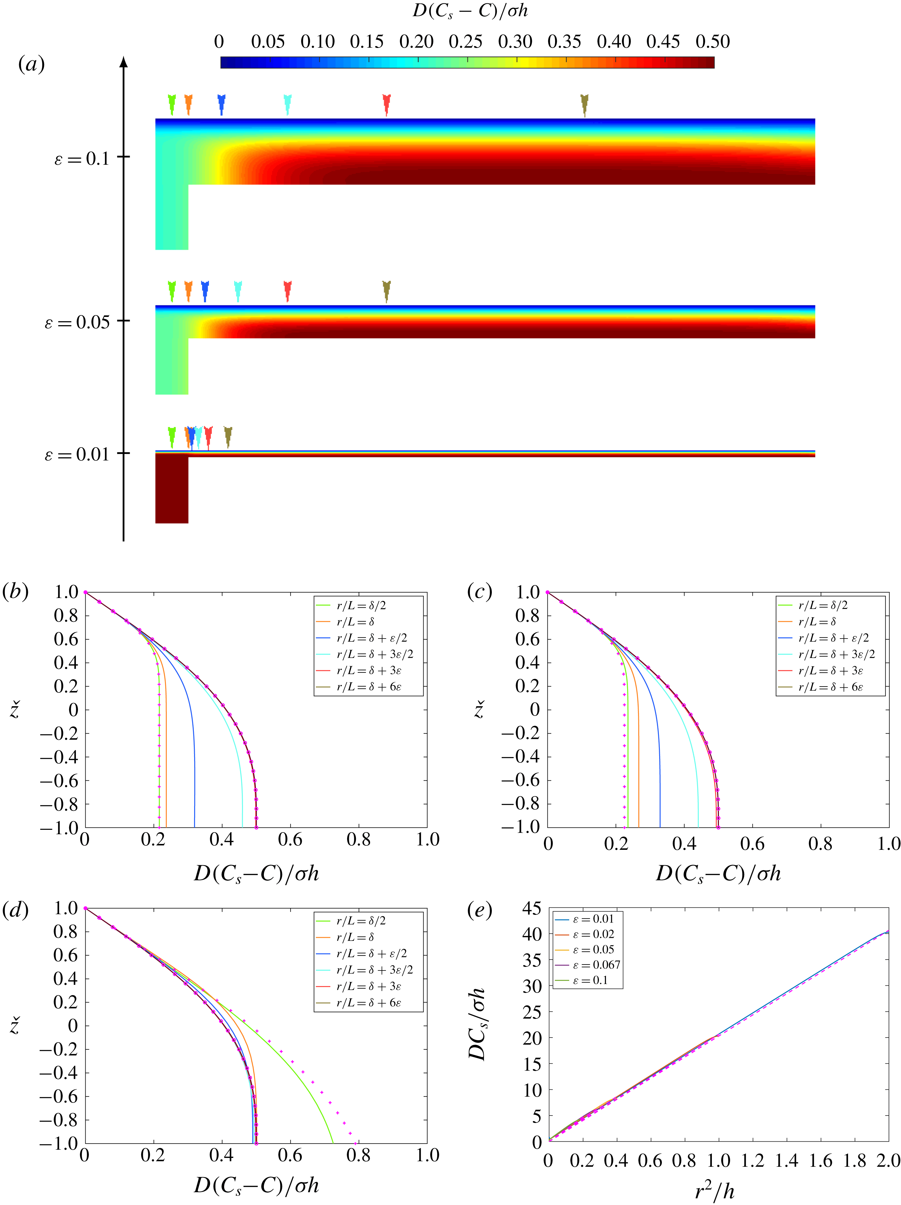
) (a) Contour distributions of the scalar field
 $C_{s}-C$
are shown for
 $Re_{p}=1$
,
 $Pe_{p}=100$
,
 $\unicode[STIX]{x1D6FF}=0.05$
and
 $\unicode[STIX]{x1D700}=0.01$
, 0.05 and 0.1. (b,c,d) Variation of the scalar
 $D(C_{s}-C)/\unicode[STIX]{x1D70E}h$
across a channel cross-section for
 $Re_{p}=1$
,
 $Pe_{p}=100$
,
 $\unicode[STIX]{x1D6FF}=0.05$
and (b)
 $\unicode[STIX]{x1D700}=0.1$
, (c)
 $\unicode[STIX]{x1D700}=0.05$
and (d)
 $\unicode[STIX]{x1D700}=0.01$
plotted at various distances from the inlet centreline (colour-coded in a). The analytical solutions in the entrance region (3.37) (
 $+$
) and channel region (3.42) (
 $\circ$
) are shown. (e) Variation of the scalar at the upper plate
 $DC_{s}/\unicode[STIX]{x1D70E}h$
with
 $r^{2}/h$
for
 $Re_{p}=1$
,
 $Pe=100$
,
 $\unicode[STIX]{x1D6FF}=0.05$
and
 $\unicode[STIX]{x1D700}=0.01$
, 0.02, 0.05, 0.067 and 0.1. The analytical solution (3.39) is plotted as a dashed line.
We now consider the scalar field when boundary condition
 $(\text{N})$
is imposed at the upper plate. The diffusive flux is prescribed and the main objective of the analysis is to determine the scalar at the upper surface
 $C_{s}(r)=C(r,h/2)$
.
3.3.1 Turning region
The solution to (3.15) that satisfies boundary condition
 $(\text{N})$
is
 $$\begin{eqnarray}\displaystyle C(r,z)=\frac{\unicode[STIX]{x1D70E}}{D^{2/3}\unicode[STIX]{x1D6FE}^{1/3}}\int _{(h/2-z)/(D/\unicode[STIX]{x1D6FE})^{1/3}}^{h}\exp \left(-\frac{\unicode[STIX]{x1D709}^{3}}{3}\right)\text{d}\unicode[STIX]{x1D709}, & & \displaystyle\end{eqnarray}$$
so that the scalar at the upper surface is
 $$\begin{eqnarray}\displaystyle C_{s}(r)=\frac{\unicode[STIX]{x1D70E}\unicode[STIX]{x0393}(1/3)}{3^{2/3}D^{2/3}\unicode[STIX]{x1D6FE}^{1/3}}. & & \displaystyle\end{eqnarray}$$
Contour distributions of the scalar and numerical and analytical scalar profiles across channel cross-sections are plotted in figure 10(a–d) for
 $Re_{p}=1$
,
 $Pe_{p}=100$
,
 $\unicode[STIX]{x1D6FF}=0.05$
and various channel aspect ratios. The analytical scalar profiles conform to the numerical solution.
3.3.2 Channel region
A separable multiplicative solution cannot satisfy boundary condition (2.13). Instead, a separable additive solution of the form
 $$\begin{eqnarray}\displaystyle C(r,z)=C_{s}(r)+{\mathcal{F}}_{c}(z), & & \displaystyle\end{eqnarray}$$
is sought. This method allows for the resolution of the full radial advection–diffusion equation analytically. The expression of
 $C_{s}$
may be determined by solving the integral form of the conservation of the scalar (3.14), which yields
 $$\begin{eqnarray}\displaystyle C_{s}(r)=\frac{\unicode[STIX]{x1D70E}}{Q/\unicode[STIX]{x03C0}-4Dh}r^{2}. & & \displaystyle\end{eqnarray}$$
The scalar at the upper plate varies proportionally to the channel surface area. The analytical solution (3.39) agrees with numerical simulations (see figure 10 e).
The expression of
 ${\mathcal{F}}_{c}$
may be determined by considering the differential form of the conservation of the scalar (2.7), which is
 $$\begin{eqnarray}\displaystyle \frac{3}{2}\frac{Q}{2\unicode[STIX]{x03C0}rh}\left(1-\frac{4z^{2}}{h^{2}}\right)\frac{\text{d}C_{s}}{\text{d}r}=D\left(\frac{1}{r}\frac{\text{d}}{\text{d}r}\left(r\frac{\text{d}C_{s}}{\text{d}r}\right)+\frac{\text{d}^{2}{\mathcal{F}}_{c}}{\text{d}z^{2}}\right). & & \displaystyle\end{eqnarray}$$
Using (3.39) yields
 $$\begin{eqnarray}\displaystyle \frac{\text{d}^{2}{\mathcal{F}}_{c}}{\text{d}z^{2}}=\frac{\unicode[STIX]{x1D70E}}{Q/\unicode[STIX]{x03C0}-4Dh}\left(\frac{3Q}{2\unicode[STIX]{x03C0}hD}\left(1-\frac{4z^{2}}{h^{2}}\right)-4\right), & & \displaystyle\end{eqnarray}$$
so that
 $$\begin{eqnarray}\displaystyle {\mathcal{F}}_{c}(z)=\frac{\unicode[STIX]{x1D70E}}{D}\left(1-\frac{8\unicode[STIX]{x1D700}}{\unicode[STIX]{x1D6FF}Pe_{p}}\right)^{-1}\left[z\left(\frac{1}{2}-\frac{4\unicode[STIX]{x1D700}}{\unicode[STIX]{x1D6FF}Pe_{p}}\right)+\frac{3z^{2}}{4h}\left(1-\frac{16\unicode[STIX]{x1D700}}{3\unicode[STIX]{x1D6FF}Pe_{p}}\right)-\frac{z^{4}}{2h^{3}}\right]_{z=h/2}^{z} & & \displaystyle\end{eqnarray}$$
or
 $$\begin{eqnarray}\displaystyle {\mathcal{F}}_{c}(z)=\frac{\unicode[STIX]{x1D70E}h}{D}\frac{{\check{z}}-1}{1-\displaystyle \frac{8\unicode[STIX]{x1D700}}{\unicode[STIX]{x1D6FF}Pe_{p}}}\left[\left(\frac{13}{32}-\frac{3\unicode[STIX]{x1D700}}{\unicode[STIX]{x1D6FF}Pe_{p}}\right)+\left(\frac{5}{32}-\frac{\unicode[STIX]{x1D700}}{\unicode[STIX]{x1D6FF}Pe_{p}}\right){\check{z}}-\frac{1}{32}\left(1+{\check{z}}\right){\check{z}}^{2}\right]. & & \displaystyle\end{eqnarray}$$
Numerical solutions for scalar profiles are plotted in figure 10(b–d) for
 $Re_{p}=1$
,
 $Pe_{p}=100$
,
 $\unicode[STIX]{x1D6FF}=0.05$
and various channel aspect ratios. They agree with the analytical solution (3.43).
4 Interior depth-averaged model
In the previous section, integral techniques were applied to examine the characteristics of the flow and scalar fields in an axisymmetric model of the turning region and part of the interior domain. In this section, this approach is extended to the full geometry consisting of one inlet and two outlets by averaging the equations for the flow and scalar transport in the cross-channel direction. The model is valid only if in (2.6), the inertial terms are negligible as compared to the viscous terms. Since the inertial and viscous terms scale as
 $\unicode[STIX]{x1D70C}u^{2}/L$
and
 $\unicode[STIX]{x1D707}u/h^{2}$
, respectively, this condition becomes
 $$\begin{eqnarray}\displaystyle Re_{p}\frac{\unicode[STIX]{x1D700}^{2}}{\unicode[STIX]{x1D6FF}}\ll 1. & & \displaystyle\end{eqnarray}$$
When
 $(\text{D})$
is imposed, the model assumes that the normalised scalar transfer coefficient is constant and equal to
 $\unicode[STIX]{x1D6EC}_{\infty }$
over the flow domain. The previous section has shown that this approximation is not always valid close to the inlet (see figure 9) and that the variation of
 $\unicode[STIX]{x1D6EC}$
across the flow domain has a dependence on
 $\unicode[STIX]{x1D6FF}$
and
 $\unicode[STIX]{x1D700}$
. It was also shown that the convergence of
 $\unicode[STIX]{x1D6EC}$
to a constant value occurs at increasing distances from the inlet centreline as
 $Pe_{p}$
increases. The accuracy of this reduced model will be assessed in § 5 using three-dimensional numerical simulations.
4.1 Integral formulation
The field variables are expressed in term of the Cartesian coordinates
 $(x,y,z)$
centred at the outlet located on the left-hand side of the inlet (as shown in figure 1
b). For convenience, they may be expressed in terms of the radial coordinate system
 $(r,\unicode[STIX]{x1D703},z)$
centred at the inlet, with the correspondence
 $$\begin{eqnarray}\displaystyle x=L\sin \left(\frac{\unicode[STIX]{x1D6FC}}{2}\right)-r\cos \unicode[STIX]{x1D703}\quad y=L\cos \left(\frac{\unicode[STIX]{x1D6FC}}{2}\right)-r\sin \unicode[STIX]{x1D703}. & & \displaystyle\end{eqnarray}$$
4.1.1 Velocity and pressure field
The velocity field is constructed in a separable form, i.e.
 $$\begin{eqnarray}\displaystyle \boldsymbol{u}(x,y,z)=\boldsymbol{u}_{h}(x,y){\mathcal{F}}_{u}({\check{z}}), & & \displaystyle\end{eqnarray}$$
where
 ${\mathcal{F}}_{u}$
is defined in (3.5). By neglecting the inertial terms in the integral form of the momentum equation, we find
 $$\begin{eqnarray}\displaystyle -\breve{\unicode[STIX]{x1D735}}p_{h}+\frac{\unicode[STIX]{x1D707}}{h^{2}}({\mathcal{F}}_{u}^{\prime }(1)-{\mathcal{F}}_{u}^{\prime }(-1))\boldsymbol{u}_{h}=\mathbf{0}, & & \displaystyle\end{eqnarray}$$
where
 $$\begin{eqnarray}\displaystyle p_{h}=\frac{1}{h}\int _{-h/2}^{h/2}p\,\text{d}z. & & \displaystyle\end{eqnarray}$$
The equation for the flow (4.4) is solved subject to the boundary conditions
 $$\begin{eqnarray}\displaystyle \hat{\boldsymbol{n}}\boldsymbol{\cdot }\boldsymbol{u}_{h}=\frac{Q}{2\unicode[STIX]{x03C0}R_{p}h}=\frac{R_{p}u_{p}}{2h},\quad \hat{\boldsymbol{n}}\boldsymbol{\cdot }\breve{\unicode[STIX]{x1D735}}\boldsymbol{u}_{h}=0, & & \displaystyle\end{eqnarray}$$
imposed respectively at the inlet and the sidewalls. The pressure at the outlets is set to have the same value, which is arbitrarily taken to be zero.
4.1.2 Scalar field with boundary condition (
$\mathit{D}$
)

The variation of the depth-averaged scalar
 $C_{h}$
is described by
 $$\begin{eqnarray}\displaystyle \unicode[STIX]{x1D6FD}_{1}\boldsymbol{u}_{h}\boldsymbol{\cdot }\breve{\unicode[STIX]{x1D735}}C_{h}=-\frac{\unicode[STIX]{x1D6EC}D}{h^{2}}C_{h}+D\breve{\unicode[STIX]{x1D735}}^{2}C_{h}, & & \displaystyle\end{eqnarray}$$
where the value
 $\unicode[STIX]{x1D6FD}_{1}=1.03$
is taken from the similarity solution in the channel region. The axisymmetric model has shown that the scalar transfer coefficient
 $\unicode[STIX]{x1D6EC}$
varies with
 $\unicode[STIX]{x1D6FF}/\unicode[STIX]{x1D700}$
and
 $Pe_{p}$
. For the numerical model,
 $\unicode[STIX]{x1D6EC}$
is imposed to be approximately constant and equal to the value that it takes away from the turning region
 $\unicode[STIX]{x1D6EC}_{\infty }=2.5694$
(see table 4).
The scalar field is subject to the boundary conditions
 $$\begin{eqnarray}\displaystyle C_{h}=1,\quad \hat{\boldsymbol{n}}\boldsymbol{\cdot }\breve{\unicode[STIX]{x1D735}}C_{h}=0, & & \displaystyle\end{eqnarray}$$
imposed respectively at the surface of the inlet and on the sidewalls.
4.1.3 Scalar field with boundary condition (
$\mathit{N}$
)

The variation of the scalar on the upper plate
 $C_{s}$
is described by
 $$\begin{eqnarray}\displaystyle \boldsymbol{u}_{h}\boldsymbol{\cdot }\breve{\unicode[STIX]{x1D735}}C_{s}=\unicode[STIX]{x1D70E}+D\breve{\unicode[STIX]{x1D735}}^{2}C_{s}. & & \displaystyle\end{eqnarray}$$
The scalar field is subject to the boundary conditions
 $$\begin{eqnarray}\displaystyle C_{s}=0,\quad \hat{\boldsymbol{n}}\boldsymbol{\cdot }\breve{\unicode[STIX]{x1D735}}C_{s}=0, & & \displaystyle\end{eqnarray}$$
imposed respectively at the surface of the inlet and the sidewalls. The diffusive flux
 $\unicode[STIX]{x1D70E}$
is chosen to be negative so that the scalar is taken up by the fluid and
 $C_{s}\geqslant 0$
.
4.2 Flow characteristics
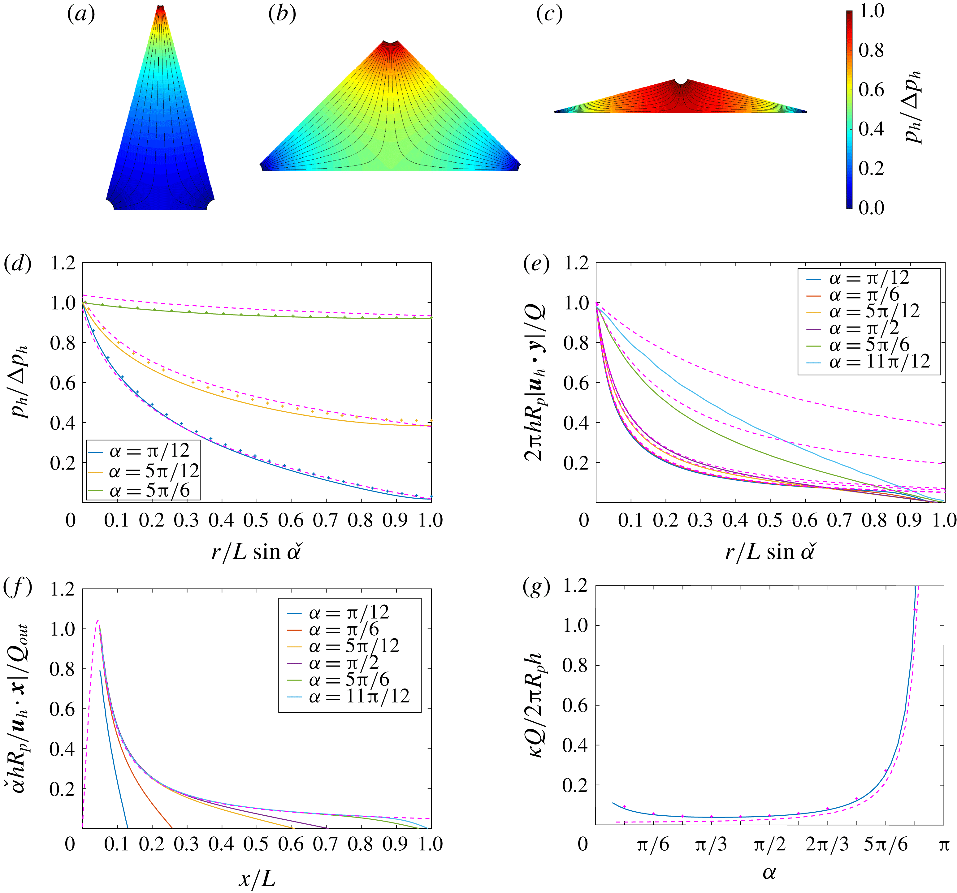
(a–c) Contour distributions of the pressure field
 $p_{h}/\unicode[STIX]{x0394}p_{h}$
are shown for fixed
 $\unicode[STIX]{x1D6FF}=0.05$
and
 $\unicode[STIX]{x1D700}=0.05$
and various apex angles (a)
 $\unicode[STIX]{x1D6FC}=\unicode[STIX]{x03C0}/6$
, (b)
 $\unicode[STIX]{x1D6FC}=\unicode[STIX]{x03C0}/2$
and (c)
 $\unicode[STIX]{x1D6FC}=5\unicode[STIX]{x03C0}/6$
. Representative streamlines are plotted on each domain. Variations of (d) the pressure
 $p_{h}/\unicode[STIX]{x0394}p_{h}$
and (e) the velocity
 $2\unicode[STIX]{x03C0}R_{p}hu_{h}/Q$
with distance from the inlet centreline along the triangle centreline for
 $\unicode[STIX]{x1D6FF}=0.05$
and various apex angles
 $\unicode[STIX]{x1D6FC}=\unicode[STIX]{x03C0}/12$
,
 $\unicode[STIX]{x03C0}/6$
,
 $5\unicode[STIX]{x03C0}/12$
,
 $\unicode[STIX]{x03C0}/2$
,
 $5\unicode[STIX]{x03C0}/6$
and
 $11\unicode[STIX]{x03C0}/12$
. The analytical solution for the pressure field (4.18) (
 $+$
) and the axisymmetric numerical solution (§ 3) (dashed lines) are plotted. (f) Variation of the velocity
 $\check{\unicode[STIX]{x1D6FC}}hR_{p}u_{h}/Q_{out}$
with distance from the outlet centreline along the separation line
 $y=0$
for
 $\unicode[STIX]{x1D6FF}=0.05$
and various apex angles where
 $\unicode[STIX]{x1D6FC}=\unicode[STIX]{x03C0}/12$
,
 $\unicode[STIX]{x03C0}/6$
,
 $5\unicode[STIX]{x03C0}/12$
,
 $\unicode[STIX]{x03C0}/2$
,
 $5\unicode[STIX]{x03C0}/6$
and
 $11\unicode[STIX]{x03C0}/12$
. The axisymmetric numerical solution (§ 3) is plotted in dashed lines. (g) Variation of the strain rate at the stagnation point
 $\unicode[STIX]{x1D705}$
normalised by
 $2\unicode[STIX]{x03C0}R_{p}h/Q$
with the apex angle
 $\unicode[STIX]{x1D6FC}$
calculated numerically (
 $+$
) and analytically using (4.11) (plain line) and (4.16) (dashed lines).
The depth-averaged velocity and pressure fields were studied in detail by Zouache et al. (Reference Zouache, Eames and Luthert2015) using both finite element methods and conformal mapping. The velocity field is expressed as
 $$\begin{eqnarray}\displaystyle u_{h} & = & \displaystyle k\frac{\displaystyle \unicode[STIX]{x1D6FD}\left(\frac{\check{\unicode[STIX]{x1D6FC}}}{\unicode[STIX]{x03C0}},\frac{\check{\unicode[STIX]{x1D6FC}}}{\unicode[STIX]{x03C0}}\right)}{4L\cos \check{\unicode[STIX]{x1D6FC}}}\nonumber\\ \displaystyle & & \displaystyle \times \,\mathit{Re}\left(\frac{\displaystyle 2{\mathcal{I}}^{-1}\left(\frac{z}{2L\cos \check{\unicode[STIX]{x1D6FC}}},\frac{\check{\unicode[STIX]{x1D6FC}}}{\unicode[STIX]{x03C0}},\frac{\check{\unicode[STIX]{x1D6FC}}}{\unicode[STIX]{x03C0}}\right)-1}{\displaystyle \left[\left(1-{\mathcal{I}}^{-1}\left(\frac{z}{2L\cos \check{\unicode[STIX]{x1D6FC}}},\frac{\check{\unicode[STIX]{x1D6FC}}}{\unicode[STIX]{x03C0}},\frac{\check{\unicode[STIX]{x1D6FC}}}{\unicode[STIX]{x03C0}}\right)\right){\mathcal{I}}^{-1}\left(\frac{z}{2L\cos \check{\unicode[STIX]{x1D6FC}}},\frac{\check{\unicode[STIX]{x1D6FC}}}{\unicode[STIX]{x03C0}},\frac{\check{\unicode[STIX]{x1D6FC}}}{\unicode[STIX]{x03C0}}\right)\right]^{\check{\unicode[STIX]{x1D6FC}}/\unicode[STIX]{x03C0}}}\right),\nonumber\\ \displaystyle & & \displaystyle\end{eqnarray}$$
where
 $z_{3}\rightarrow \infty$
,
 $\unicode[STIX]{x1D6FD}$
is the beta function,
 ${\mathcal{I}}^{-1}$
is the inverse regularised incomplete beta function (Abramowitz & Stegun Reference Abramowitz and Stegun1972),
 $\check{\unicode[STIX]{x1D6FC}}=\unicode[STIX]{x03C0}/2-\unicode[STIX]{x1D6FC}/2$
and
 $$\begin{eqnarray}\displaystyle k=\frac{2\unicode[STIX]{x1D6FC}LR_{p}u_{p}\cos \check{\unicode[STIX]{x1D6FC}}}{\displaystyle \unicode[STIX]{x1D6FD}\left(\frac{\check{\unicode[STIX]{x1D6FC}}}{\unicode[STIX]{x03C0}},\frac{\check{\unicode[STIX]{x1D6FC}}}{\unicode[STIX]{x03C0}}\right)h\int _{\unicode[STIX]{x03C0}+\check{\unicode[STIX]{x1D6FC}}}^{2\unicode[STIX]{x03C0}-\check{\unicode[STIX]{x1D6FC}}}\left|\frac{\displaystyle 2{\mathcal{I}}^{-1}\left(\frac{\text{e}^{\text{i}\check{\unicode[STIX]{x1D6FC}}}+\unicode[STIX]{x1D6FF}\text{e}^{\text{i}\unicode[STIX]{x1D703}}}{2\cos \check{\unicode[STIX]{x1D6FC}}},\frac{\check{\unicode[STIX]{x1D6FC}}}{\unicode[STIX]{x03C0}},\frac{\check{\unicode[STIX]{x1D6FC}}}{\unicode[STIX]{x03C0}}\right)-1}{\displaystyle \left[\left(1-{\mathcal{I}}^{-1}\left(\frac{\text{e}^{\text{i}\check{\unicode[STIX]{x1D6FC}}}+\unicode[STIX]{x1D6FF}\text{e}^{\text{i}\unicode[STIX]{x1D703}}}{2\cos \check{\unicode[STIX]{x1D6FC}}},\frac{\check{\unicode[STIX]{x1D6FC}}}{\unicode[STIX]{x03C0}},\frac{\check{\unicode[STIX]{x1D6FC}}}{\unicode[STIX]{x03C0}}\right)\right){\mathcal{I}}^{-1}\left(\frac{\text{e}^{\text{i}\check{\unicode[STIX]{x1D6FC}}}+\unicode[STIX]{x1D6FF}\text{e}^{\text{i}\unicode[STIX]{x1D703}}}{2\cos \check{\unicode[STIX]{x1D6FC}}},\frac{\check{\unicode[STIX]{x1D6FC}}}{\unicode[STIX]{x03C0}},\frac{\check{\unicode[STIX]{x1D6FC}}}{\unicode[STIX]{x03C0}}\right)\right]^{\check{\unicode[STIX]{x1D6FC}}/\unicode[STIX]{x03C0}}}\right|\,\text{d}\unicode[STIX]{x1D703}}. & & \displaystyle \nonumber\\ \displaystyle & & \displaystyle\end{eqnarray}$$
The velocity field close to the inlet is well-described by the axisymmetric model analysed in § 3.2.2. As
 $\unicode[STIX]{x1D6FC}\rightarrow 0$
, the domain tends to the pure axisymmetric configuration so that the agreement with the axisymmetric model extends quite far from the inlet. As
 $\unicode[STIX]{x1D6FC}\rightarrow \unicode[STIX]{x03C0}$
, the extent to which the model is valid becomes limited to the direct vicinity of the inlet (see figure 11
e). This is a consequence of the reduction of the distance between the inlet and the stagnation line (
 $y=0$
), which causes the flow over most of the flow domain to be dominated by an irrotational straining flow. In the outlet region, the flow is a dominantly radial flow. Mass conservation requires that the flow rate at the outlets
 $Q_{out}$
satisfy
 $$\begin{eqnarray}\displaystyle Q_{out}=\frac{\unicode[STIX]{x1D6FC}}{4\unicode[STIX]{x03C0}}Q=\frac{\unicode[STIX]{x1D6FC}R_{p}^{2}u_{p}}{4}. & & \displaystyle\end{eqnarray}$$
The axisymmetric model applies accurately to the velocity field in the vicinity of the outlet, as illustrated in figure 11(f), which shows the evolution of the radial velocity with radial distance from the outlet centreline along the separation line
 $y=0$
.
There is one stagnation point in the depth-averaged formulation located on the separation line
 $y=0$
halfway between the two outlets. The fluid particle residence time in the vicinity of this point is long and this has a significant influence on the scalar distribution. Close to the stagnation point, the flow is dominantly an irrotational straining flow where the velocity, to leading order, is
 $$\begin{eqnarray}\displaystyle u_{x}=\unicode[STIX]{x1D705}x,\quad u_{y}=-\unicode[STIX]{x1D705}y, & & \displaystyle\end{eqnarray}$$
where
 $\unicode[STIX]{x1D705}$
is the strain rate, which can be determined from (4.11). A reasonable estimate of the strain rate may be obtained by considering the variation of the flow velocity centred on the stagnation point along the separation line
 $y=0$
, which is approximately
 $$\begin{eqnarray}\displaystyle u_{x}\simeq \frac{Q}{2\unicode[STIX]{x03C0}h(x-L\sin (\unicode[STIX]{x1D6FC}/2))}+\frac{Q}{2\unicode[STIX]{x03C0}h(x+L\sin (\unicode[STIX]{x1D6FC}/2))}. & & \displaystyle\end{eqnarray}$$
The strain rate estimate is then
 $$\begin{eqnarray}\displaystyle \unicode[STIX]{x1D705}=\left.\frac{\unicode[STIX]{x2202}u_{x}}{\unicode[STIX]{x2202}x}\right|_{x\rightarrow 0}\simeq \frac{Q}{\unicode[STIX]{x03C0}hL^{2}\sin ^{2}(\unicode[STIX]{x1D6FC}/2)}. & & \displaystyle\end{eqnarray}$$
Figure 11(g) shows the variation of the normalised strain rate
 $\unicode[STIX]{x1D705}Q/2\unicode[STIX]{x03C0}R_{p}h$
with
 $\unicode[STIX]{x1D6FC}$
. The approximate expression (4.16) conforms closely with both analytical (4.11) and numerical solutions. The strain rate is minimal for
 $\unicode[STIX]{x1D6FC}=\unicode[STIX]{x03C0}/3$
and increases rapidly as
 $\unicode[STIX]{x1D6FC}\rightarrow \unicode[STIX]{x03C0}$
(see figure 11
g). To make explicit the interdependence between the geometrical parameters
 $\unicode[STIX]{x1D6FF}$
,
 $\unicode[STIX]{x1D700}$
,
 $\unicode[STIX]{x1D6FC}$
and
 $L$
and the strain rate at the stagnation point, equation (4.16) may be recast as
 $$\begin{eqnarray}\displaystyle \frac{\unicode[STIX]{x1D705}}{u_{p}/L}\simeq \frac{\unicode[STIX]{x1D6FF}^{2}}{\unicode[STIX]{x1D700}\sin ^{2}(\unicode[STIX]{x1D6FC}/2)}. & & \displaystyle\end{eqnarray}$$
The pressure field is (Zouache et al. Reference Zouache, Eames and Luthert2015)
 $$\begin{eqnarray}\displaystyle p_{h}=-k\log \left|\frac{\displaystyle \left({\mathcal{I}}^{-1}\left(\frac{x+\text{i}y}{2L\cos \check{\unicode[STIX]{x1D6FC}}},\frac{\check{\unicode[STIX]{x1D6FC}}}{\unicode[STIX]{x03C0}},\frac{\check{\unicode[STIX]{x1D6FC}}}{\unicode[STIX]{x03C0}}\right)-z_{3}\right)}{\displaystyle \sqrt{{\mathcal{I}}^{-1}\left(\frac{x+\text{i}y}{2L\cos \check{\unicode[STIX]{x1D6FC}}},\frac{\check{\unicode[STIX]{x1D6FC}}}{\unicode[STIX]{x03C0}},\frac{\check{\unicode[STIX]{x1D6FC}}}{\unicode[STIX]{x03C0}}\right)\left({\mathcal{I}}^{-1}\left(\frac{x+\text{i}y}{2L\cos \check{\unicode[STIX]{x1D6FC}}},\frac{\check{\unicode[STIX]{x1D6FC}}}{\unicode[STIX]{x03C0}},\frac{\check{\unicode[STIX]{x1D6FC}}}{\unicode[STIX]{x03C0}}\right)-1\right)}}\right|, & & \displaystyle\end{eqnarray}$$
so that the pressure drop
 $\unicode[STIX]{x0394}p_{h}$
may be calculated by subtracting the average pressure at the inlet from the one averaged over an outlet. The analytical solution for the pressure field conforms closely to both the numerical solution and the axisymmetric model (see figure 11
d). Figure 11(a–c), which shows the contour distribution of the pressure field for various apex angles, illustrates the dependence of the pressure distribution on the parameter
 $\unicode[STIX]{x1D6FC}$
. For fixed
 $\unicode[STIX]{x1D6FF}$
and
 $\unicode[STIX]{x1D700}$
, when
 $\unicode[STIX]{x1D6FC}\ll \unicode[STIX]{x03C0}$
most of the pressure drop occurs close to the inlet (figure 11
a). For larger values of
 $\unicode[STIX]{x1D6FC}$
, the regions with the largest pressure drop are in the direct vicinity of the outlets (figure 11
b,c).
4.3 Scalar field with boundary condition (
$\mathit{D}$
)

For sufficiently large Péclet numbers (e.g.
 $Pe_{p}\geqslant 100$
), the inlet scalar extends beyond the turning region and into the channel region. The scalar field is then decomposed into two regions; the inlet region and the straining flow region close to the separation surface. The dominant transport mechanism in these two regions is different. The transition between the two regions occurs at the distance from the inlet where the flow becomes a dominantly straining flow and is therefore a function of
 $\unicode[STIX]{x1D6FC}$
(see figure 11
g).
4.3.1 Inlet region
In this region, the model reduces to the axisymmetric model laid down in § 3.2.2. For
 $Pe_{p}\gg 1$
the transport of the scalar is dominantly advective and described by
 $$\begin{eqnarray}\displaystyle \boldsymbol{u}_{h}\boldsymbol{\cdot }\breve{\unicode[STIX]{x1D735}}C_{h}\simeq -\frac{\unicode[STIX]{x1D6EC}_{\infty }D}{\unicode[STIX]{x1D6FD}_{1}h^{2}}C_{h}. & & \displaystyle\end{eqnarray}$$
Solving (4.19) along a streamline yields (Zouache et al. Reference Zouache, Eames, Klettner and Luthert2016)
 $$\begin{eqnarray}\displaystyle C_{h}(x,y)=C_{h}(x_{0},y_{0})\exp \left(-\frac{\unicode[STIX]{x1D6EC}_{\infty }D}{\unicode[STIX]{x1D6FD}_{1}h^{2}}\unicode[STIX]{x0394}T\right), & & \displaystyle\end{eqnarray}$$
where
 $\unicode[STIX]{x0394}T(x_{0},y_{0};x,y)$
is the fluid residence time between
 $(x_{0},y_{0})$
and
 $(x,y)$
. The diffusive flux is then
 $$\begin{eqnarray}\displaystyle j_{d}=\frac{\unicode[STIX]{x1D6EC}_{\infty }D}{h}C_{h}=\frac{\unicode[STIX]{x1D6EC}_{\infty }DC_{h}(x_{0},y_{0})}{h}\exp \left(-\frac{\unicode[STIX]{x1D6EC}_{\infty }D}{\unicode[STIX]{x1D6FD}_{1}h^{2}}\unicode[STIX]{x0394}T\right). & & \displaystyle\end{eqnarray}$$
For narrow domains, an approximate analytical expression of the residence time of a fluid particle released at the inlet surface is (Zouache et al. Reference Zouache, Eames and Luthert2015)
 $$\begin{eqnarray}\displaystyle \unicode[STIX]{x0394}T(r)\simeq \frac{2\unicode[STIX]{x03C0}h}{Q}\int _{R_{p}}^{r}r\,\text{d}r=\frac{\unicode[STIX]{x03C0}h}{Q}(r^{2}-R_{p}^{2}), & & \displaystyle\end{eqnarray}$$
which retrieves (3.35).
(Boundary condition
 $\text{D}$
) (a–f) Contour distributions of the scalar field
 $C_{h}$
for fixed
 $\unicode[STIX]{x1D700}=0.05$
,
 $\unicode[STIX]{x1D6FF}=0.05$
, (a,b,c)
 $Pe_{p}=100$
, (d,e,f)
 $Pe_{p}=1000$
and varying apex angles (a,d)
 $\unicode[STIX]{x1D6FC}=\unicode[STIX]{x03C0}/6$
, (b,e)
 $\unicode[STIX]{x03C0}/2$
and (c,f)
 $5\unicode[STIX]{x03C0}/6$
when condition
 $(\text{D})$
is imposed. (g) Variation of the scalar along the triangle centreline with distance from the inlet centreline for fixed
 $\unicode[STIX]{x1D700}=0.05$
,
 $\unicode[STIX]{x1D6FF}=0.05$
and various
 $\unicode[STIX]{x1D6FC}=\unicode[STIX]{x03C0}/12$
,
 $\unicode[STIX]{x03C0}/6$
,
 $5\unicode[STIX]{x03C0}/12$
,
 $\unicode[STIX]{x03C0}/2$
,
 $5\unicode[STIX]{x03C0}/6$
and
 $11\unicode[STIX]{x03C0}/12$
and
 $Pe_{p}=100$
(plain lines) and
 $Pe_{p}=1000$
(dash-dotted lines). The analytical expression of
 $C_{h}$
(3.25) obtained with the axisymmetric model is plotted as a dashed line. (h) Variation of the scalar field
 $C_{h}$
in the straining region with distance from the separation surface shown for fixed
 $\unicode[STIX]{x1D700}=0.05$
,
 $\unicode[STIX]{x1D6FF}=0.05$
and various
 $\unicode[STIX]{x1D6FC}=\unicode[STIX]{x03C0}/2$
,
 $2\unicode[STIX]{x03C0}/3$
and
 $5\unicode[STIX]{x03C0}/6$
. The scalar was expressed relative to the scalar at the separation surface
 $C_{h}^{sep}$
and normalised by
 $C_{h}^{0}-C_{h}^{sep}$
.

Departure from this model is determined by the angle
 $\unicode[STIX]{x1D6FC}$
(see figure 12
g). As
 $\unicode[STIX]{x1D6FC}\rightarrow \unicode[STIX]{x03C0}$
the extent to which (4.21) applies reduces to the direct vicinity of the inlet.
4.3.2 Straining region
For simple flows, the velocity near the stagnation point is given by (4.14). In the vicinity of the separation surface, the transport of the scalar in the vertical direction is dominant over the transport in the direction parallel to the separation surface. The conservation of the scalar (4.7) is therefore reduced to
 $$\begin{eqnarray}\displaystyle \frac{\text{d}^{2}C_{h}}{\text{d}y^{2}}+\frac{\unicode[STIX]{x1D6FD}_{1}\unicode[STIX]{x1D705}}{D}y\frac{\text{d}C_{h}}{\text{d}y}-\frac{\unicode[STIX]{x1D6EC}_{\infty }}{h^{2}}C_{h}=0, & & \displaystyle\end{eqnarray}$$
subject to the boundary conditions
 $$\begin{eqnarray}\displaystyle C_{h}(x_{0},y_{0})=C_{h}(r_{0})=C_{h}^{0},\quad \left.\frac{\text{d}C_{h}}{\text{d}y}\right|_{y=0}=0, & & \displaystyle\end{eqnarray}$$
where
 $C_{h}^{0}$
may be determined by using (4.20). (4.23) admits for solution
 $$\begin{eqnarray}\displaystyle C_{h}=C_{h}^{0}\exp \left(-\frac{\unicode[STIX]{x1D6FD}_{1}\unicode[STIX]{x1D705}}{2D}(y^{2}-y_{0}^{2})\right)\frac{\displaystyle \text{}_{1}{\mathcal{H}}_{1}\left(-\frac{1}{2}-\frac{\unicode[STIX]{x1D6EC}_{\infty }D}{2\unicode[STIX]{x1D6FD}_{1}h^{2}\unicode[STIX]{x1D705}};\frac{1}{2};\frac{\unicode[STIX]{x1D6FD}_{1}\unicode[STIX]{x1D705}}{2D}y^{2}\right)}{\displaystyle \text{}_{1}{\mathcal{H}}_{1}\left(-\frac{1}{2}-\frac{\unicode[STIX]{x1D6EC}_{\infty }D}{2\unicode[STIX]{x1D6FD}_{1}h^{2}\unicode[STIX]{x1D705}};\frac{1}{2};\frac{\unicode[STIX]{x1D6FD}_{1}\unicode[STIX]{x1D705}}{2D}y_{0}^{2}\right)}, & & \displaystyle\end{eqnarray}$$
where
 $_{1}{\mathcal{H}}_{1}$
is the Kummer confluent hypergeometric function (Abramowitz & Stegun Reference Abramowitz and Stegun1972). The diffusive flux is then
 $$\begin{eqnarray}\displaystyle j_{d}=\frac{\unicode[STIX]{x1D6EC}_{\infty }DC_{h}^{0}}{h}\exp \left(-\frac{\unicode[STIX]{x1D6FD}_{1}\unicode[STIX]{x1D705}}{2D}(y^{2}-y_{0}^{2})\right)\frac{\displaystyle \text{}_{1}{\mathcal{H}}_{1}\left(-\frac{1}{2}-\frac{\unicode[STIX]{x1D6EC}_{\infty }D}{2\unicode[STIX]{x1D6FD}_{1}h^{2}\unicode[STIX]{x1D705}};\frac{1}{2};\frac{\unicode[STIX]{x1D6FD}_{1}\unicode[STIX]{x1D705}}{2D}y^{2}\right)}{\displaystyle \text{}_{1}{\mathcal{H}}_{1}\left(-\frac{1}{2}-\frac{\unicode[STIX]{x1D6EC}_{\infty }D}{2\unicode[STIX]{x1D6FD}_{1}h^{2}\unicode[STIX]{x1D705}};\frac{1}{2};\frac{\unicode[STIX]{x1D6FD}_{1}\unicode[STIX]{x1D705}}{2D}y_{0}^{2}\right)}. & & \displaystyle\end{eqnarray}$$
A Taylor series expansion for
 $y\ll 1$
yields
 $$\begin{eqnarray}\displaystyle & \displaystyle C_{h}\simeq \frac{\displaystyle C_{h}^{0}\exp \left(\frac{\unicode[STIX]{x1D6FD}_{1}\unicode[STIX]{x1D705}}{2D}y_{0}^{2}\right)}{\displaystyle \text{}_{1}{\mathcal{H}}_{1}\left(-\frac{1}{2}-\frac{\unicode[STIX]{x1D6EC}_{\infty }D}{2\unicode[STIX]{x1D6FD}_{1}h^{2}\unicode[STIX]{x1D705}};\frac{1}{2};\frac{\unicode[STIX]{x1D6FD}_{1}\unicode[STIX]{x1D705}}{2D}y_{0}^{2}\right)}\left(1+\frac{\unicode[STIX]{x1D6EC}_{\infty }}{2h^{2}}y^{2}\right). & \displaystyle\end{eqnarray}$$
 $$\begin{eqnarray}\displaystyle & \displaystyle j_{d}\simeq \frac{\displaystyle \unicode[STIX]{x1D6EC}_{\infty }DC_{h}^{0}\exp \left(\frac{\unicode[STIX]{x1D6FD}_{1}\unicode[STIX]{x1D705}}{2D}y_{0}^{2}\right)}{\displaystyle \text{}_{1}{\mathcal{H}}_{1}\left(-\frac{1}{2}-\frac{\unicode[STIX]{x1D6EC}_{\infty }D}{2\unicode[STIX]{x1D6FD}_{1}h^{2}\unicode[STIX]{x1D705}};\frac{1}{2};\frac{\unicode[STIX]{x1D6FD}_{1}\unicode[STIX]{x1D705}}{2D}y_{0}^{2}\right)h}\left(1+\frac{\unicode[STIX]{x1D6EC}_{\infty }}{2h^{2}}y^{2}\right). & \displaystyle\end{eqnarray}$$
Figure 12(g) shows the variation of the scalar in the boundary layer in the vicinity of the separation surface for
 $Pe_{p}=1000$
and various values of
 $\unicode[STIX]{x1D6FC}$
. The analytical solution (4.25) conforms closely with the numerical solution.
4.4 Scalar field with boundary condition (
$\mathit{N}$
)

Similar methods may be applied to the case where
 $(\text{N})$
is imposed. The scalar field is decomposed into an inlet region and a straining region.
4.4.1 Inlet region
The scalar in the vicinity of the inlet is described by the axisymmetric model laid down in § 3.3.2. The extent to which this model extends is the same as when (
 $\text{D}$
) is imposed (see figure 13).
4.4.2 Straining region
In the vicinity of the separation surface region, the conservation of the scalar (4.9) reduces to
 $$\begin{eqnarray}\displaystyle -\unicode[STIX]{x1D705}y\frac{\text{d}C_{s}}{\text{d}y}=\unicode[STIX]{x1D70E}+D\frac{\text{d}^{2}C_{s}}{\text{d}y^{2}}, & & \displaystyle\end{eqnarray}$$
which may be recast as
 $$\begin{eqnarray}\displaystyle \frac{\text{d}}{\text{d}y}\left[\frac{\text{d}C_{s}}{\text{d}y}\exp \left(\frac{\unicode[STIX]{x1D705}}{2D}y^{2}\right)\right]=-\frac{\unicode[STIX]{x1D70E}}{D}\exp \left(\frac{\unicode[STIX]{x1D705}}{2D}y^{2}\right). & & \displaystyle\end{eqnarray}$$
By imposing
 $C_{s}(0)=C_{s}^{0}$
, equation (4.30) admits for solution
 $$\begin{eqnarray}\displaystyle C_{s}=C_{s}^{0}-\frac{\unicode[STIX]{x1D70E}}{D}\int _{0}^{y}\int _{0}^{\unicode[STIX]{x1D709}}\exp \left(-\frac{\unicode[STIX]{x1D705}}{2D}(\unicode[STIX]{x1D709}^{2}-\unicode[STIX]{x1D701}^{2})\right)\text{d}\unicode[STIX]{x1D701}\,\text{d}\unicode[STIX]{x1D709} & & \displaystyle\end{eqnarray}$$
or
 $$\begin{eqnarray}\displaystyle C_{s}=C_{s}^{0}+\sqrt{\frac{\unicode[STIX]{x03C0}D}{2\unicode[STIX]{x1D705}}}\text{erf}\left(\sqrt{\frac{\unicode[STIX]{x1D705}}{2D}}y\right)-\frac{\unicode[STIX]{x1D70E}}{2D}y^{2}\displaystyle \text{}_{2}{\mathcal{H}}_{2}\left([1,1];\left[\frac{3}{2},2\right];-\frac{\unicode[STIX]{x1D705}}{2D}y^{2}\right), & & \displaystyle\end{eqnarray}$$
where
 $\text{erf}$
is the error function and
 $\text{}_{2}{\mathcal{H}}_{2}$
is the generalised hypergeometric function (Abramowitz & Stegun Reference Abramowitz and Stegun1972).
[Boundary condition
 $\text{N}$
] (a–c) Contour distributions of the scalar at the upper plate
 $DC_{s}/\unicode[STIX]{x1D70E}h$
for fixed
 $\unicode[STIX]{x1D700}=0.05$
,
 $\unicode[STIX]{x1D6FF}=0.05$
,
 $Pe_{p}=100$
and varying apex angles (a)
 $\unicode[STIX]{x1D6FC}=\unicode[STIX]{x03C0}/6$
, (b)
 $\unicode[STIX]{x03C0}/2$
and (c)
 $5\unicode[STIX]{x03C0}/6$
when condition
 $(\text{N})$
is imposed. (d) Variation of the scalar
 $DC_{s}/\unicode[STIX]{x1D70E}h$
along the triangle centreline with distance from the inlet centreline for fixed
 $\unicode[STIX]{x1D700}=0.05$
,
 $\unicode[STIX]{x1D6FF}=0.05$
,
 $Pe_{p}=100$
and varying apex angles
 $\unicode[STIX]{x1D6FC}=\unicode[STIX]{x03C0}/12$
,
 $\unicode[STIX]{x03C0}/6$
,
 $5\unicode[STIX]{x03C0}/12$
,
 $\unicode[STIX]{x03C0}/2$
,
 $5\unicode[STIX]{x03C0}/6$
and
 $11\unicode[STIX]{x03C0}/12$
(plain lines). The analytical expression of
 $C_{s}$
(3.39) obtained for the axisymmetric model is plotted as a dashed line. (e) Variation of the scalar
 $C_{s}/C_{s}^{0}$
, where
 $C_{s}^{0}=C_{s}(0)$
, in the straining region along the triangle centreline with distance from the separation surface for fixed
 $\unicode[STIX]{x1D700}=0.05$
,
 $\unicode[STIX]{x1D6FF}=0.05$
,
 $Pe_{p}=100$
and varying apex angles
 $\unicode[STIX]{x1D6FC}=\unicode[STIX]{x03C0}/12$
,
 $\unicode[STIX]{x03C0}/6$
,
 $5\unicode[STIX]{x03C0}/12$
,
 $\unicode[STIX]{x03C0}/2$
,
 $5\unicode[STIX]{x03C0}/6$
and
 $11\unicode[STIX]{x03C0}/12$
. The analytical expression (4.32) is plotted as a dashed line.

In the limit
 $\unicode[STIX]{x1D705}/\unicode[STIX]{x1D70E}\ll 1$
, an approximate expression of
 $C_{s}$
is
 $$\begin{eqnarray}\displaystyle C_{s}\simeq C_{s}^{0}-\frac{\unicode[STIX]{x1D70E}}{2D}y^{2}. & & \displaystyle\end{eqnarray}$$
Expression (4.32) conforms closely with the numerical solution (see figure 13 e).
5 Three-dimensional model
The aim of this section is to test the validity of the axisymmetric model (§ 3) and the depth-averaged model (§ 4) against three-dimensional numerical calculations. The range of geometrical parameters
 $\unicode[STIX]{x1D6FF}$
and
 $\unicode[STIX]{x1D700}$
for which the momentum equation and the conservation of the scalar were solved is indicated in figure 2(b). For each set of parameters
 $\unicode[STIX]{x1D6FF}$
and
 $\unicode[STIX]{x1D700}$
, eleven values of
 $\unicode[STIX]{x1D6FC}$
were considered (
 $\unicode[STIX]{x03C0}/12\leqslant \unicode[STIX]{x1D6FC}\leqslant 11\unicode[STIX]{x03C0}/12$
), and the equations were solved for
 $Re_{p}=0.1$
, 1 and 10. The conservation of the scalar was then solved for
 $Pe_{p}=0.1$
, 1, 100 and 1000.
5.1 Flow characteristics
(a,b) Representative streamlines and (c,d) contour distributions of the pressure field
 $p/\unicode[STIX]{x0394}p_{t}$
calculated for fixed
 $\unicode[STIX]{x1D6FF}=0.05$
,
 $\unicode[STIX]{x1D700}=0.05$
and
 $Re_{p}=1$
are plotted for (a,c)
 $\unicode[STIX]{x1D6FC}=\unicode[STIX]{x03C0}/3$
and (b,d)
 $\unicode[STIX]{x1D6FC}=5\unicode[STIX]{x03C0}/6$
. (e) Variation of the depth-averaged velocity
 $2\unicode[STIX]{x03C0}hR_{p}u_{h}/Q$
across the central plane and a side plane calculated using the three-dimensional (plain lines) and axisymmetric (dashed lines) models shown for fixed
 $\unicode[STIX]{x1D6FF}=0.05$
,
 $\unicode[STIX]{x1D700}=0.05$
and
 $\unicode[STIX]{x1D6FC}=\unicode[STIX]{x03C0}/3$
. Inset: variation of the velocity profile
 $2\unicode[STIX]{x03C0}hR_{p}u/\unicode[STIX]{x1D705}|x-L\cos \check{\unicode[STIX]{x1D6FC}}|Q$
across a cross-section of the separation surface calculated at various distances from the stagnation line using the three-dimensional model (plain lines) for fixed
 $\unicode[STIX]{x1D6FF}=0.05$
,
 $\unicode[STIX]{x1D700}=0.05$
and
 $\unicode[STIX]{x1D6FC}=\unicode[STIX]{x03C0}/3$
. The analytical profile (5.4) is plotted as
 $+$
. (f) Variation of the dimensionless pressure drop
 $\unicode[STIX]{x03C0}L^{3}\unicode[STIX]{x0394}p_{t}/2\unicode[STIX]{x1D707}Q$
across the channel region (in red) and the entire flow domain (in black) with
 $\unicode[STIX]{x1D6FC}$
are shown for fixed
 $\unicode[STIX]{x1D6FF}=0.05$
and
 $\unicode[STIX]{x1D700}=0.05$
and
 $Re_{p}=0.1$
, 1 and 10. Analytical solutions for the channel region (4.18) (dotted lines) and the full domain (5.2) (plain line) are shown.

Contours of the pressure field and representative streamlines calculated for fixed
 $\unicode[STIX]{x1D6FF}=0.05$
,
 $\unicode[STIX]{x1D700}=0.05$
and
 $Re_{p}=1$
and the two apex angles
 $\unicode[STIX]{x1D6FC}=\unicode[STIX]{x03C0}/3$
and
 $5\unicode[STIX]{x03C0}/6$
are shown in figure 14(a–d). Numerical calculations agree closely with the axisymmetric and the depth-averaged models. They confirm that in addition to being controlled by the relative values of
 $\unicode[STIX]{x1D6FF}$
and
 $\unicode[STIX]{x1D700}$
, the pressure field is also controlled by
 $\unicode[STIX]{x1D6FC}$
. Over the range of parameters considered, this dependence is described well by (4.18).
The pressure drop may be estimated by extending the semi-empirical approach implemented in § 3.1 to the three-dimensional geometry. The pressure drop across a pipe of length
 $L_{p}$
is given by (3.8). Using the relation between the inlet and outlet flow rates (4.13), the contributions of the outlet pipes to the total pressure drop are estimated to be
 $$\begin{eqnarray}\displaystyle \unicode[STIX]{x0394}p_{p}=\frac{16\unicode[STIX]{x1D707}L_{p}Q_{out}}{\check{\unicode[STIX]{x1D6FC}}R_{p}^{4}}=\frac{8\unicode[STIX]{x1D6FC}\unicode[STIX]{x1D707}L_{p}Q}{\check{\unicode[STIX]{x1D6FC}}\unicode[STIX]{x03C0}R_{p}^{4}}. & & \displaystyle\end{eqnarray}$$
The pressure drop
 $\unicode[STIX]{x0394}p_{c}$
in the channel region is
 $\unicode[STIX]{x0394}p_{c}=\unicode[STIX]{x0394}p_{h}$
, where
 $\unicode[STIX]{x0394}p_{h}$
is given in (4.18). Expression (4.18) agrees with the numerical solution of the pressure drop across the channel region for
 $Re_{p}=0.1$
and
 $Re_{p}=1$
and for
 $Re_{p}=10$
when flow separation does not occur (
 $\unicode[STIX]{x1D6FF}/\unicode[STIX]{x1D700}\gg 1$
) (see figure 14
f). The pressure drop over the totality of the flow domain is estimated by adding the pressure drop in the inlet and outlet pipes (2.9) and in the channel region, i.e.
 $$\begin{eqnarray}\displaystyle \frac{\unicode[STIX]{x03C0}L^{3}\unicode[STIX]{x0394}p_{t}}{2\unicode[STIX]{x1D707}Q}=\frac{L_{p}}{L}\frac{4}{\unicode[STIX]{x1D6FF}^{4}}\left(1+\frac{\unicode[STIX]{x1D6FC}}{\check{\unicode[STIX]{x1D6FC}}}\right)+\frac{\unicode[STIX]{x03C0}L^{3}\unicode[STIX]{x0394}p_{h}}{2\unicode[STIX]{x1D707}Q}. & & \displaystyle\end{eqnarray}$$
This relation describes the interdependence between the inlet and outlet pipe radii, the thickness of the channel region and the relative distribution of inlets and outlets as described by the angle
 $\unicode[STIX]{x1D6FC}$
. When
 $\unicode[STIX]{x1D6FC}\ll \unicode[STIX]{x03C0}$
,
 $\unicode[STIX]{x1D6FC}/\check{\unicode[STIX]{x1D6FC}}\rightarrow 0$
and the pressure drop in the channel region is approximately (Zouache et al.
Reference Zouache, Eames and Luthert2015)
 $$\begin{eqnarray}\displaystyle \unicode[STIX]{x0394}p_{c}\simeq -\frac{6Q\unicode[STIX]{x1D707}}{\unicode[STIX]{x03C0}h^{3}}\log \unicode[STIX]{x1D6FF}, & & \displaystyle\end{eqnarray}$$
which retrieves (3.9). Relation (5.2) conforms closely to numerical solutions (see figure 14 f).
The velocity field close to the inlet and outlets is entirely described by the axisymmetric model for all values of
 $\unicode[STIX]{x1D6FF}$
,
 $\unicode[STIX]{x1D700}$
and
 $\unicode[STIX]{x1D6FC}$
(see figure 14
e). Within the channel region, when
 $\unicode[STIX]{x1D700}\leqslant 0.1$
and
 $Re_{p}\leqslant 1$
the depth-averaged model agrees with numerical solutions both close to the inlet and outlets and in the straining region. Close to the stagnation surface, the velocity is parabolic and satisfies
 $$\begin{eqnarray}\displaystyle u_{x}=\frac{3}{2}\unicode[STIX]{x1D705}(x-\cos \check{\unicode[STIX]{x1D6FC}})(1-{\check{z}}^{2}),\quad u_{y}=\frac{3}{2}\unicode[STIX]{x1D705}y(1-{\check{z}}^{2}),\quad u_{z}=0, & & \displaystyle\end{eqnarray}$$
where
 $\unicode[STIX]{x1D705}$
is the strain rate defined in the depth-averaged model. Velocity profiles across the separation surface calculated at increasing distances from the stagnation line are plotted for
 $\unicode[STIX]{x1D6FF}=0.05$
,
 $\unicode[STIX]{x1D700}=0.05$
and
 $\unicode[STIX]{x1D6FC}=\unicode[STIX]{x03C0}/3$
in the inset to figure 14(e). For larger Reynolds number (e.g.
 $Re_{p}=10$
), the inertial terms in the integral form of the momentum equation cannot be neglected, and the depth-averaged model is not valid.
Contour distribution of (a,b) the horizontal and (c,d) the vertical component of the vorticity field
 $2\unicode[STIX]{x03C0}R_{p}h^{2}\unicode[STIX]{x1D74E}/Q$
plotted across vertical and horizontal sections of the flow domain, respectively, for fixed
 $\unicode[STIX]{x1D6FF}=0.05$
and
 $\unicode[STIX]{x1D700}=0.05$
, (a,c)
 $\unicode[STIX]{x1D6FC}=\unicode[STIX]{x03C0}/3$
and (b,d)
 $\unicode[STIX]{x1D6FC}=5\unicode[STIX]{x03C0}/6$
.

The important spatial variations in the dominant features of the flow across the turning and channel regions are manifest when considering the vorticity field. The three components of the vorticity field are
 $$\begin{eqnarray}\displaystyle \unicode[STIX]{x1D714}_{x}=-\frac{\unicode[STIX]{x2202}u_{y}}{\unicode[STIX]{x2202}z}=\frac{12z}{h^{2}}u_{h},\quad \unicode[STIX]{x1D714}_{y}=\frac{\unicode[STIX]{x2202}u_{x}}{\unicode[STIX]{x2202}z}=-\frac{12z}{h^{2}}u_{h},\quad \unicode[STIX]{x1D714}_{z}=\frac{\unicode[STIX]{x2202}u_{y}}{\unicode[STIX]{x2202}x}-\frac{\unicode[STIX]{x2202}u_{x}}{\unicode[STIX]{x2202}y}=0, & & \displaystyle\end{eqnarray}$$
(Batchelor Reference Batchelor1957). Close to the inlet,
 $u_{h}\simeq Q/2\unicode[STIX]{x03C0}hr$
so that (3.11) is retrieved and the vorticity field conforms to the axisymmetric model (see figure 15). On the separation surface, the vertical vorticity is non-zero because of the slip condition; however, because the velocity normal to the separation surface is zero no horizontal vorticity is generated.
5.2 Scalar field with boundary condition (
$\mathit{D}$
)

[Boundary condition
 $\text{D}$
] (a–d) Contour distributions of the scalar field
 $C$
across vertical sections of the flow domain when
 $(\text{D})$
is imposed are shown for fixed
 $\unicode[STIX]{x1D6FF}=0.05$
,
 $\unicode[STIX]{x1D700}=0.05$
,
 $Re_{p}=1$
, (a,c)
 $\unicode[STIX]{x1D6FC}=\unicode[STIX]{x03C0}/3$
and (b,d)
 $\unicode[STIX]{x1D6FC}=5\unicode[STIX]{x03C0}/6$
. The Péclet number was fixed (a,b)
 $Pe_{p}=100$
and (c,d)
 $Pe_{p}=1000$
. (e,f) Variation of the depth-averaged scalar
 $C_{h}$
with distance from the inlet centreline along the centre plane and (inset) a side plane, shown for (e)
 $\unicode[STIX]{x1D6FC}=\unicode[STIX]{x03C0}/3$
and (f)
 $\unicode[STIX]{x1D6FC}=5\unicode[STIX]{x03C0}/6$
, fixed values
 $\unicode[STIX]{x1D6FF}=0.05$
,
 $\unicode[STIX]{x1D700}=0.05$
,
 $Re_{p}=1$
and
 $Pe_{p}=100$
and
 $Pe_{p}=1000$
. The solutions from the axisymmetric model are plotted as dashed lines.
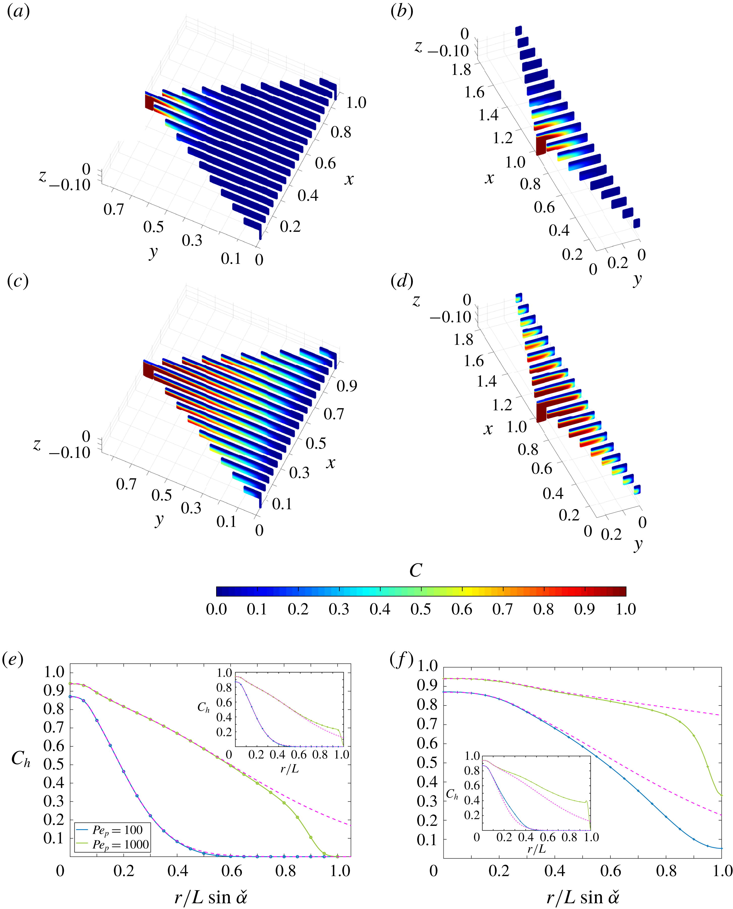
Contours of the scalar field generated for fixed
 $\unicode[STIX]{x1D6FF}=0.05$
,
 $\unicode[STIX]{x1D700}=0.05$
,
 $Re_{p}=1$
and
 $Pe=100$
and 1000 and
 $\unicode[STIX]{x1D6FC}=\unicode[STIX]{x03C0}/3$
and
 $5\unicode[STIX]{x03C0}/6$
are shown in figure 16(a–d). The associated variation of
 $C_{h}$
with distance from the inlet centreline along the central plane and a side plane are shown in figure 16(e,f). The numerical solutions for both the scalar field and the scalar transfer coefficient agree with the axisymmetric model close to the inlet for all geometries and values of
 $Pe_{p}$
(see figures 16
a–d and 17
a).
Because the depth-averaged model relies on the assumption that the normalised scalar coefficient
 $\unicode[STIX]{x1D6EC}$
is constant and equal to
 $\unicode[STIX]{x1D6EC}_{\infty }$
(see § 4.3), its validity is entirely determined by the variation of
 $\unicode[STIX]{x1D6EC}$
across the channel region. This in turn is a function of
 $\unicode[STIX]{x1D6FC}$
and the relative values of
 $\unicode[STIX]{x1D6FF}$
and
 $\unicode[STIX]{x1D700}$
. For moderate Péclet numbers (e.g.
 $Pe_{p}\leqslant 100$
),
 $\unicode[STIX]{x1D6EC}$
converges to
 $\unicode[STIX]{x1D6EC}_{\infty }$
at a short distance from the inlet for all values of
 $\unicode[STIX]{x1D6FF}$
,
 $\unicode[STIX]{x1D700}$
and
 $\unicode[STIX]{x1D6FC}$
so that the depth-averaged model conforms closely to the three-dimensional simulations. For large Péclet numbers (e.g.
 $Pe_{p}=1000$
), the convergence of
 $\unicode[STIX]{x1D6EC}$
to
 $\unicode[STIX]{x1D6EC}_{\infty }$
is much slower. The depth-averaged model underestimates the scalar density flux
 $j_{d}$
over most of the channel region, which causes the scalar field
 $C_{h}$
to be overestimated. When
 $|\unicode[STIX]{x1D6FC}-\unicode[STIX]{x03C0}|\ll 1$
,
 $\unicode[STIX]{x1D6EC}$
does not converge to a constant value within the channel region (see figure 17
b).
[Boundary condition
 $\text{D}$
] Variation of the scalar transfer coefficient with distance from the inlet centreline along the centre plane and (inset) a side plane are shown for (a)
 $\unicode[STIX]{x1D6FC}=\unicode[STIX]{x03C0}/3$
and (b)
 $\unicode[STIX]{x1D6FC}=5\unicode[STIX]{x03C0}/6$
, fixed values
 $\unicode[STIX]{x1D6FF}=0.05$
,
 $\unicode[STIX]{x1D700}=0.05$
,
 $Re_{p}=1$
and
 $Pe_{p}=100$
and
 $Pe_{p}=1000$
when
 $(\text{D})$
is imposed. The solutions from the axisymmetric model are plotted as dashed lines.
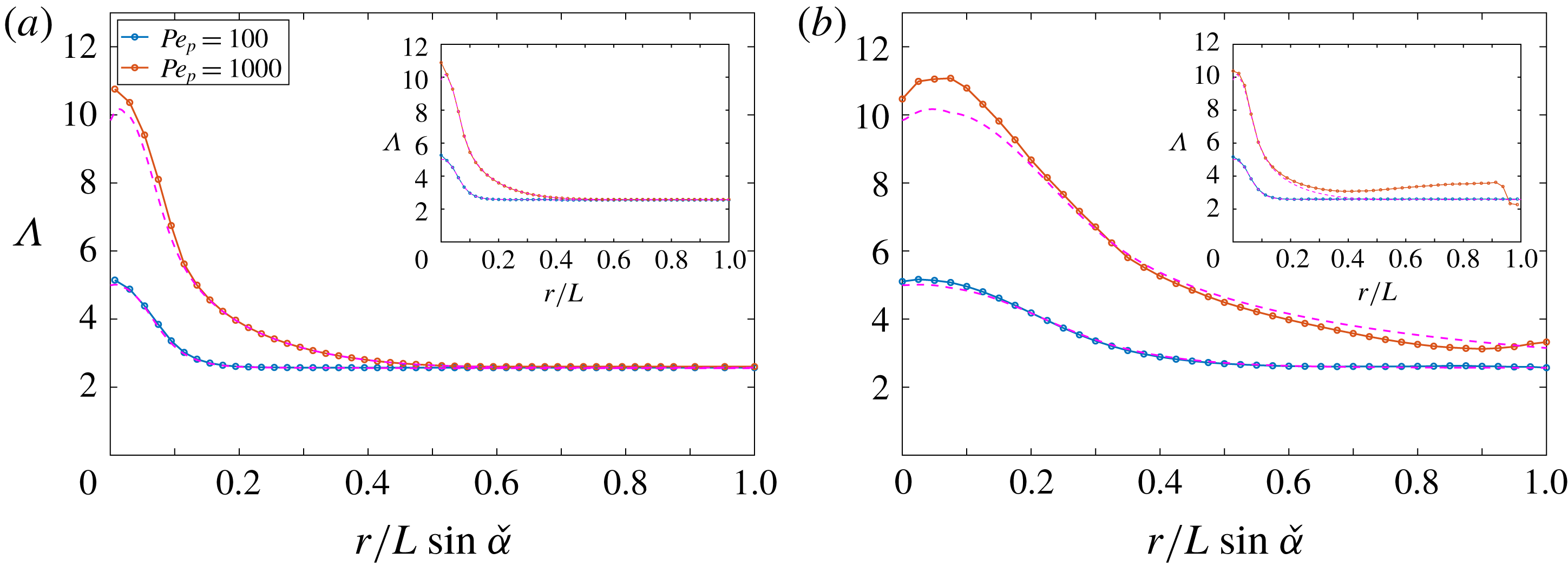
5.3 Scalar field with boundary condition (
$\mathit{N}$
)

Contours of the scalar field generated for fixed
 $\unicode[STIX]{x1D6FF}=0.05$
,
 $\unicode[STIX]{x1D700}=0.05$
,
 $Re_{p}=1$
and
 $Pe=100$
and
 $\unicode[STIX]{x1D6FC}=\unicode[STIX]{x03C0}/3$
and
 $5\unicode[STIX]{x03C0}/6$
are shown in figure 18(a,b). The associated variation of the scalar at the upper plate
 $C_{s}$
with distance from the inlet centreline along either the central plane or a side plane are shown in figures 18(c) and 18(d), respectively. Both the axisymmetric model and the depth-averaged model conform to the three-dimensional model in the turning region and the channel region for all values of
 $\unicode[STIX]{x1D6FF}$
,
 $\unicode[STIX]{x1D700}$
and
 $\unicode[STIX]{x1D6FC}$
. In the straining region the variation of
 $C_{s}$
is in good agreement with the analytical model (4.32). For all geometries, the maximal value of
 $C_{s}$
is obtained at the stagnation point.
[Boundary condition
 $\text{N}$
] (a,b) Contour distributions of the normalised scalar field
 $DC/\unicode[STIX]{x1D70E}h$
across vertical sections of the flow domain when
 $(\text{N})$
is imposed are shown for fixed
 $\unicode[STIX]{x1D6FF}=0.05$
,
 $\unicode[STIX]{x1D700}=0.05$
, (a)
 $\unicode[STIX]{x1D6FC}=\unicode[STIX]{x03C0}/3$
, (b)
 $\unicode[STIX]{x1D6FC}=5\unicode[STIX]{x03C0}/6$
. The Péclet number was fixed
 $Pe_{p}=100$
. (c,d) Variation of the scalar at the upper plate
 $DC_{s}/\unicode[STIX]{x1D70E}h$
with distance from the inlet centreline along (c) the centre plane and (d) the side plane shown for fixed
 $\unicode[STIX]{x1D6FF}=0.05$
,
 $\unicode[STIX]{x1D700}=0.05$
,
 $Pe_{p}=100$
and various
 $\unicode[STIX]{x1D6FC}=\unicode[STIX]{x03C0}/3$
and
 $5\unicode[STIX]{x03C0}/6$
. The solution from the axisymmetric model (dashed lines) and from the 2D analysis in the straining region (dotted lines) are plotted.

6 Discussion and conclusions
This paper lays down the first comprehensive description of the flow and transport of a passive scalar in multipolar flows. Every fundamental aspect of the geometry of multipolar configurations has been incorporated into the analysis. The study applies to an arbitrary number of poles and to any distribution of inlets and outlets. The topology of multipolar flows has been harnessed by reducing the flow domain to a subset of the flow field so that the analysis has been carried out over bounded domains. The key geometrical parameters – the inlet/outlet pipe aspect ratio
 $\unicode[STIX]{x1D6FF}$
, the channel aspect ratio
 $\unicode[STIX]{x1D700}$
and the angle between an inlet and two outlets
 $\unicode[STIX]{x1D6FC}$
– have been considered over a wide range of values and their impact on the flow and scalar fields has been analysed systematically. The results are valid for
 $Re_{p}\leqslant 10$
and
 $0.1\leqslant Pe_{p}\leqslant 1000$
; however, they can be extended to
 $Re_{p}\leqslant 60$
if
 $\unicode[STIX]{x1D6FF}/\unicode[STIX]{x1D700}\ll 1$
or
 $\unicode[STIX]{x1D6FF}/\unicode[STIX]{x1D700}\gg 1$
. An important novelty of this work is that the three-dimensional geometry of multipolar configurations has been considered in its entirety. This has allowed for the identification of regions with distinct flow and scalar transfer properties. Separate models have been developed for the turning region, the channel region and the straining region within the channel region. For each model, both numerical and analytical solutions have been formulated and conform closely to each other.
A summary of the local characteristics of the flow field is drawn in figure 19(a). The flow in the turning region is dominantly a viscous straining flow when
 $\unicode[STIX]{x1D6FF}\gg \unicode[STIX]{x1D700}$
and an irrotational straining flow when
 $\unicode[STIX]{x1D6FF}\leqslant \unicode[STIX]{x1D700}$
. In the channel region, the flow close to the inlet and outlets is axisymmetric and respectively source- or sink-dominated. In the straining region the flow is a dominantly irrotational straining flow that has a dependence on the relative arrangement of the inlet and outlets.
Summary of the characteristics of (a) the flow, (b) the scalar field when condition (
 $\text{D}$
) is imposed at the upper plate and (c) the scalar field when condition (
 $\text{N}$
) is imposed at the upper plate.

The scalar field has been analysed in the limit where transfers can be modelled either by setting a constant scalar field at the upper plate (
 $\text{D}$
) or by imposing a constant flux (
 $\text{N}$
) across the upper surface of the flow domain. The local properties of the scalar field when either of these boundary conditions is imposed are summarised in figure 19(b,c). The scalar field associated with each boundary condition has different properties, which are a natural consequence of the characteristics of the flow field. When (
 $\text{D}$
) is imposed, most of the transfers occur in the direct vicinity of the inlet, which corresponds to the region where the flow is the fastest – and the fluid residence time is the shortest (Zouache et al.
Reference Zouache, Eames and Luthert2015). In contrast, when (
 $\text{N}$
) is imposed, the largest increase in the scalar field occurs in the vicinity of the separation surface, where the flow is the slowest – and the fluid residence time is the largest (Zouache et al.
Reference Zouache, Eames and Luthert2015).
In most practical applications of multipolar configurations, the boundary condition is likely to be a weighted combination of (
 $\text{D}$
) and (
 $\text{N}$
) of the form
 $$\begin{eqnarray}\displaystyle aC+b(\boldsymbol{n}\boldsymbol{\cdot }\unicode[STIX]{x1D735}C)=d, & & \displaystyle\end{eqnarray}$$
where
 $a$
,
 $b$
are non-zero constants and
 $d$
is a function defined on the surface across which transfers occur. The limits for which (
 $\text{D}$
) or (
 $\text{N}$
) are good approximations of (6.1) not only depend on
 $\unicode[STIX]{x1D6FF}$
and
 $\unicode[STIX]{x1D700}$
, but also on factors external to the flow domain such as the physical characteristics of the interface across which transfers occur and the scalar field away from the fluid. For instance, in thin channels, large scalar gradients perpendicular to the upper plate cause the scalar field at this wall to be comparatively smaller so that (
 $\text{N}$
) may be an appropriate approximation of (6.1). Since scalar gradients are smaller in thick channels, (
 $\text{D}$
) is a more appropriate approximation when
 $\unicode[STIX]{x1D700}\gg 1$
. Considering scalar gradients external to the flow domain when selecting a boundary condition is crucial in the context of mass transport in the back of the eye. The transport of oxygen across the outer part of the retina is driven by concentration gradients perpendicular to the interface between the retina and the microvasculature that sustains it, the choriocapillaris. Experimental studies have shown that oxygen concentration may be assumed to be constant at the interface between choriocapillaris and retina (Haugh, Linsenmeier & Goldstick Reference Haugh, Linsenmeier and Goldstick1990). A Dirichlet boundary condition is therefore an adequate approximate boundary condition for this interface. However, this condition would not be appropriate to investigate dynamic changes in oxygen transport caused by alterations in the blood flow or in the structure of the retina, which are known to occur in ageing and disease. In this instance, the balance between oxygen concentration and gradients may be modified, and (6.1) would be more accurate.
The present work has shown that straining regions are particularly important to both local and global scalar transport and transfer processes. In the turning region, the transfer density flux
 $j_{d}$
and the scalar at the upper plate
 $C_{s}$
are a function of the strain rate, which is itself determined by the ratio
 $\unicode[STIX]{x1D6FF}/\unicode[STIX]{x1D700}$
. In the separation surface region, they are a function of the strain rate
 $\unicode[STIX]{x1D705}$
. The large-scale (irrotational) straining flow region close to the separation surface coincides with a diffusion-limited region and involves a large fluid residence time. This straining region has properties similar to the borders between choriocapillaris lobules observed during dye angiography, which consists of the imaging of the transport of a passive fluorescent dye in the choriocapillaris (Zouache et al.
Reference Zouache, Eames, Klettner and Luthert2016). They have also been experimentally observed and harnessed in microfluidic systems to maintain a non-uniform concentration field (Qasaimeh et al.
Reference Qasaimeh, Gervais and Juncker2011).
By considering the geometry of multipolar flows in its entirety, it has been possible to describe the intricate relationship between global geometrical and flow parameters and local scalar transport properties. In the turning region, the strain rate is a key determinant of the scalar field and is a function of
 $\unicode[STIX]{x1D6FF}/\unicode[STIX]{x1D700}$
. This ratio also determines the strain rate in the separation surface region – and therefore the thickness of the scalar boundary layer – through relation (4.17). The thickness of this boundary layer (and also the scalar transfer in this region) may be varied by changing the apex angle, since the strain rate
 $\unicode[STIX]{x1D705}$
varies with
 $\unicode[STIX]{x1D6FC}$
. In effect, the present analysis describes how the geometrical parameters
 $\unicode[STIX]{x1D6FF}$
,
 $\unicode[STIX]{x1D700}$
and
 $\unicode[STIX]{x1D6FC}$
may be varied to adjust local transfer properties. This result may be taken further by considering the variations of the strain rates
 $\unicode[STIX]{x1D6FE}$
and
 $\unicode[STIX]{x1D705}$
with
 $\unicode[STIX]{x1D6FF}$
,
 $\unicode[STIX]{x1D700}$
and
 $\unicode[STIX]{x1D6FC}$
. At constant flow rate, the variation of the scalar transfer density flux in the turning region with
 $\unicode[STIX]{x1D6FF}/\unicode[STIX]{x1D700}$
admits a maximum when (
 $\text{D}$
) is imposed. Similarly, the evolution of
 $C_{s}$
in the turning region with
 $\unicode[STIX]{x1D6FF}/\unicode[STIX]{x1D700}$
admits a minimum when (
 $\text{N}$
) is imposed. In the separation surface region,
 $j_{d}$
and
 $C_{s}$
may also be maximised or minimised respectively because of the variation of
 $\unicode[STIX]{x1D705}$
with
 $\unicode[STIX]{x1D6FF}$
,
 $\unicode[STIX]{x1D700}$
and
 $\unicode[STIX]{x1D6FC}$
. The present analysis therefore demonstrates how the geometry of multipolar configurations may be optimised to control scalar transfers.
The present work lays the foundation for more specific studies and practical investigations of multipolar flows, as some aspects of the geometry, flow and scalar transport have been idealised. The geometry of the turning region has been simplified by imposing a right angle between inlet and outlet pipes and the plane of the plates. Previous work has shown that inlet bends reduce pressure losses across the inlet of radial diffusers, prevent flow separation, and could therefore be used to optimise the inlet geometry (Moller Reference Moller1966; Nakabayashi et al.
Reference Nakabayashi, Ichikawa and Morinishi2002). The assumption of independence between the scalar field, the viscosity and the density of the fluid is satisfied only when the ranges of variation in temperature or mass within the fluid are small. In the context of heat transfers fluids with temperature-dependent viscosity may affect channel flows in many ways, including their linear stability (Potter & Graber Reference Potter and Graber1972; Ockendon & Ockendon Reference Ockendon and Ockendon1977; Shäfer & Herwig Reference Shäfer and Herwig1993; Wall & Wilson Reference Wall and Wilson1996; Wall & Nagata Reference Wall and Nagata2000; Sameen & Govindarajan Reference Sameen and Govindarajan2007), which would ultimately affect heat transfers under both
 $(\text{D})$
and
 $(\text{N})$
. The surface across which transfers have been considered has been simplified. Heat transfers across a rough surface have been shown to have a dependence on both viscosity and diffusivity of the fluid (Owen & Thomson Reference Owen and Thomson1962).
Future work will focus on applying our findings to refine our understanding of the movement of oxygen, nutrients and metabolism by-products in the back of the eye and to the design of cooling devices. In both fields of application, our main objective will be to gather experimental evidence demonstrating how the geometry of multipolar flows may be adjusted to optimise bulk and local heat or mass transfers.
Acknowledgements
The authors gratefully acknowledge the support of the Leverhulme Trust Research Project Grant RPG-2015-276. The authors also acknowledge the use of the University College London Grace High Performance Computing Facility (Grace@UCL), and associated support services, in the completion of this work. C.A.K. acknowledges support from the European Research Council under the European Union’s Seventh Framework Programme (FP7/20072013)/ERC grant agreement number 336084, awarded to Professor Tiziana Rossetto (UCL). I.E. and P.J.L. acknowledge the support from the National Institute for Health Research (NIHR) Biomedical Research Centre at Moorfields Eye Hospital NHS Foundation Trust and UCL Institute of Ophthalmology, London.