

Introduction
Remote sensing images from different origins offer an unprecedented monitoring capacity for agriculture fields (Mulla, Reference Mulla2013). They provide field information over time with image resolution ranging from a few centimetres to 5 m. In Europe, with the INSPIRE Directive (http://inspire.ec.europa.eu/) national geographic institutes make available to all citizens large data sets of remote sensing images. This is the case in France with the French National Institute of Geographic and Forest Information (IGN) which makes available (https://www.geoportail.gouv.fr/) historical airborne images regularly acquired in the visible range over the last 80 years. The Google company also offers via the Google Earth software, visible images regularly updated with access to historical images. The availability and the temporal resolution of remote sensing images is expected to increase with the emergence of new projects like Sentinel (Battude et al., Reference Battude, Al Bitar, Morin, Cros, Huc, Sicre and Demarez2016) or Planet (Houborg & McCabe, Reference Houborg and McCabe2016). Until today, these image data sets have been little used in precision agriculture. Indeed, they have significant drawbacks since the acquisition date is not controlled and does not necessarily match with optimal stage of the crops. Moreover, currently available images are mostly captured in the visible range and common informative indices (i.e. NDVI) can’t be calculated. However, given the resolution of the images, they are likely to provide valuable information to delineate temporally stable zones, especially for a perennial crop like vines.
In a context of massive image production by many stakeholders, the potential of these available images to support growers in delineating soil within field zones seems a relevant question. Similar questions have already been investigated in the literature. Heijting et al. (Reference Heijting, de Bruin and Bregt2011) demonstrated how the spatial knowledge that farmers have of their fields could be a starting point to map the within-field variation of soil properties. The combined use of the farmer’s expertise with high-resolution data to define within field zones may therefore constitute a relevant approach. Fleming et al. (Reference Fleming, Heermann and Westfall2004) have already shown that soil colour and soil apparent electrical conductivity maps were relevant to assist the farmer in defining management areas.
The objective of this work is to test the ability of visible historical remote sensing images to support the growers in delineating soil zones corresponding to potential management zones. An experiment was performed on three vine fields in a vineyard located in southern France.
Material and method
Field description
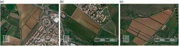
The study was carried out in 2016 on three blocks of wine production located near Montpellier (Villeneuve-lès-Maguelone, France 43°31'52.668''N, 3°51'51.597''W, RGF93). The blocks (Fig. 1) are called Argel, Arnel and Larzat and are shown respectively in Figure 1a, 1b and 1c. Blocks area ranged from 2 ha for Arnel to 7.2 ha for Larzat. The blocks were composed of different fields with different grape varieties. As the experimentation focuses on the within field soil variability, different grape varieties will not be describe further. Vine field were planted between 2004 and 2010 and were subjected to very classical training systems in southern France (Vertical shoot positioning with a 2.5 m inter-row and mechanical weeding). They were non-irrigated.
Blocks with fields used for the experiment, (a) Argel, (b) Arnel and (c) Larzat.

Remote sensing images used
For each block, the time series of remote sensing images were taken from Google Earth and Geoportail (IGN, France) platforms. All of them were freely available for a non-commercial use. Images were georeferenced (when necessary) and integrated in a GIS project (QGIS, Quantum GIS Development, V2.12, Open Source Geospatial Foundation Project) to be overlaid with the borders of the blocks. Twelve images spread over a period ranging from 1960 to 2014 were available on the three blocks considered. Images were all visible images with variable spatial resolutions (~0.5–5 m.). Most images were RGB images except some old historical images which were in black and white. Images were acquired at very different times of the year and present different stage like vegetation images and bare soil images. Therefore they did not necessarily correspond to optimal observation dates.
Zones delineation
Zones were delineated by the head of the vineyard, called ‘expert’ in the rest of the document. The expert was in charge of the vineyard since 2000. Over 16 years, he developed a very good knowledge of blocks and their spatial variability. Indeed, he regularly performed field surveys to carry out or to advise on the implementation of various technical operations (soil sampling, soil tillage, weeding, pruning, harvest, etc.).
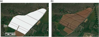
Two zoning methods based on the knowledge of the expert were carried out. On each block a first zoning was performed without any images (ZP). A second zoning was carried out with the support of free remote sensing images (ZAI). Both methods aimed at providing expert within-field zones. In order to avoid any influence of the first zoning (ZP) over the second one (ZAI) a break of two weeks was considered between the two steps. To avoid any disturbance with technological issues, expert zone delineation was performed on printed maps with pens of different colours. Zone borders and their labels were written down by the expert himself. The two zoning methods differed in the type of information provided to the expert during zones delineation. For ZP zoning (first zoning), only the fields’ borders were available with surrounding information (roads, other fields, etc.). Surrounding information was provided by visible remote sensing images. As shown Figure 2a, any within field information eventually brought were hidden by a white mask. Surrounding information was kept as a support for expert orientation and localisation. For ZAI zoning (second zoning), a transparency plastic with printed field borders (all fields of a block) was given to the expert. Similarly to ZP, ZAI zoning was performed with colour pens by the expert himself. All available historical images were printed and given to the expert who had the possibility to superimpose the transparency plastic on each of them (Fig. 2b). The transparency plastic was therefore the medium which the expert could draw zones taking into account information highlighted by remote sensing images chosen as a background.
Example of supporting information used to carry out ZP zoning (a) with a white mask of the fields hiding any potential information brought by images and ZAI zoning (b) with the results of expert zone delineation performed on superimposed transparency plastic.

Information described by zoning
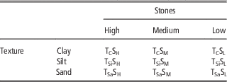
As a first attempt, experiments focused on soil composition. Two major reasons justified this choice. First, Fleming et al. (Reference Fleming, Heermann and Westfall2004) already showed the ability of soil colour to delineate relevant expert zones along with farmers’ knowledge, raising potential interest in soil colour information provided by visible images to delineate relevant within field zones. Second, soil composition is a key parameter to consider for site specific management, and testing the relevance of historical remote sensing images to delineate within field zones is therefore of paramount importance for the wine industry. Based on a first meeting with the expert, two variables were considered as significant indicators of soil variability in the specific conditions of the experiment: presence of stones and soil texture. In order to ease zone labelling, three classes were defined for each of the indicators. Indicators and their considered classes are summarized Table 1.
Classification used to define expert zones according to the soil characteristics: Stones and texture (clay, silt and sand content)

Note that in this work, the objective of the zoning was not to provide zones that could be directly used for site specific management but zones that may explain differences. Depending on the operations under consideration or on the basis of additional information, zones may or may not be managed site specifically.
Zoning validation
In order to validate the relevance of the expert zones and to allow their objective comparison, measurements of apparent soil electrical conductivity (ECa) were carried out on each block. ECa was chosen for its ability to provide relevant information on soil texture variability (Corwin, Plant, Reference Corwin and Plant2005) and also for the possibility to have a spatial resolution allowing zones to be validated. Measurements were performed on a regular sampling grid of 15 m x 15 m for each block with an EM38 (Geonics Ltd, Ontario, Canada). Measurements were made in a single day for each block in April and June 2016. A GPS receiver (E-trex, Garmin, Olathe, Kansas, USA) with an embedded EGNOS signal correction was used to georeference ECa measurements. EM38 was located in the middle of the interrow and alongside the rows. All trellises were in nylon in the fields so electrical effects of metallic trellises (D.W. Lamb, Reference Lamb, Mitchell and Hyde2005) were not present.
Data analysis
In order to analyse the soil variability and to characterize the potential spatial organisation of the soil variability, a semi-variogram analysis was performed on ECa data for each block using the GeoFIS software (V1.0, INRA / IRSTEA / Montpellier SupAgro, France). Within field zones as drawn by the expert either on paper maps (for ZP approach) or on transparency plastic (for ZAI approach) were manually digitized and geo-refenced using the field borders. Once digitized, zone contours were integrated as a specific data layer in a GIS project with all available spatial data. The GIS project contained all available spatial data (historical remote sensing images, field borders, ECa data, and expert zones) allowing spatial analysis to be performed. Spatial analysis was performed with the QGIS software (Quantum GIS Development, V2.12, Open Source Geospatial Foundation Project).
The performance (or ability) of the different zoning approaches (ZP or ZAI) to explain soil variability was assessed with the weighted variance reduction approach as proposed by Brobryk et al. (Reference Bobryk, Myers, Kitchen, Shanahan, Sudduth, Drummond and Gomez Raboteaux2016). The variance reduction was calculated with ECa data considered as the ground truth for soil variability. The advantage of this approach is that it provided a single value that could be easily compared between zoning methodologies. The area-weighted ECa variances
 $\sigma _{s}^{2} $
of each block and each zoning were calculated as (Eq. 1):
 $$\sigma _{s}^{2} \,{\equals}\,\mathop{\sum}\limits_1^n {\sigma _{i} .\omega _{i} } $$
Where
 $\omega _{i} $
is the proportion of the field area contained within the ith zone, and
 $\sigma _{i} $
is the variance within I
 $$
 $\in$
[1,n] zones resulting from the considered expert zoning delineation methods (ZP or ZAI). The variance reduction (Rv) is then calculated for each block and each type of expert zoning methods as follow (Eq. 2):
 $$R_{v} \,{\equals}\,1{\minus}\left( {{{\sigma _{s}^{2} } \over {\sigma _{{WF}}^{2} }}} \right)$$
Where
 $\sigma _{{WF}}^{2} $
is the total variance of the ECa measurements in the block. The variance reduction R
v
was used to obtain an objective comparison of expert zonings.
As a result, for each block the comparison of the two indices Rv (ZP) and Rv (ZAI) was used in order to quantify the added value of information eventually brought by remote sensing images to improve expert zoning.
Results and discussion
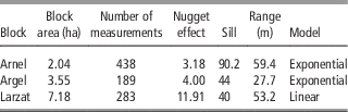
Table 2 shows the results of the semi-variogram analysis performed on ECa data for the three blocks. All blocks present a spatially organised variability in ECa values which is highlighted by exponential or linear semi-variogram models with a clear sill different from the nugget effect and the presence of a range. Assuming ECa is a good surrogate for soil texture, this result shows the opportunity to delineate within field soil zones for the three blocks. Note however that blocks exhibit strong differences. Arnel block presents the highest partial sill (sill - nugget effect) with a significant range showing a large opportunity to define within field zones. Larzat block presents a lower partial sill with a high nugget effect which may due to a significant short range variability (not fully captured by our sampling grid) which may be problematic to define a relevant zoning. Finally the Argel block presents a small range which may also constitute a limit to define relevant soil zones. This diversity is however interesting to test the robustness of the approach under different situations.
Spatial characteristics of apparent electrical conductivity of the three studied blocks

Expert zoning evaluation
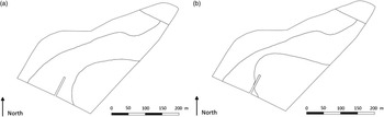
Figure 3 shows an example of the different zones defined by the expert on the Arnel block with ZP and ZAI methods. Both zonings are quite similar in the number of zones and the general shape of zones. Figure 3 shows how colour information of remote sensing images was used by the expert to refine contour zones as defined in the previous step (ZP zoning) when no information was available and that zones were defined only from the knowledge of the expert.
Example of ZP Zoning (a) and ZAI zoning (b) performed on the Larzat block.

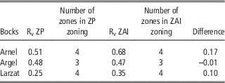
Table 3 shows the variance reduction (Rv) observed for the three blocks with ZP and ZAI zoning approaches. Results are quite different from one block to another. Except for Argel block, the consideration of remote sensing information improves the ability of expert zoning to explain ECa variability; this was shown by the difference in variance reduction between ZP and ZAI approaches. Note however, that for Argel block, the reduction in ECa-variance can be considered as similar either with ZP or ZAI approach. For Larzat and Arnel, reduction in ECa-variance is higher with the ZAI zoning approach, highlighting the value of remote sensing information to refine expert defined zones. Results in ECa variance reduction have also to be compared with ECa within field variability (Table 3). Indeed, ECa variance reduction is the highest for Arnel block which exhibits the highest structured variability. In this case, ZAI zoning significantly improved the expert zoning. Conversely, ECa variance reduction is logically the lowest for Argel block which exhibits a high nugget effect. In this case ZAI zoning didn’t improve the expert zoning. Table 3 highlights several important points. First, the expert (like many growers) has a strong knowledge of the within field variability of his blocks. This is explained by the relatively small size of vine fields compared to arable crop fields and the large number of manual operations which require him to walk through the block several times a year and necessarily to observe its environment. These characteristics explained the ability of the ZP zoning approach to explain the within field soil variability in our experiment. Secondly, information brought by remote sensing images may constitute relevant information to refine and quantify expert knowledge, thus explaining the ability of ZAI approach to better explain the within field variability in the majority of the cases. Finally, whatever the considered zoning approach, its relevancy is determined by the spatial variability exhibited by the blocks, which is important in such experiments since zoning is irrelevant when spatial variability is randomly distributed.
Rv index of ZP and ZAI zonings of the three blocks Arnel, Argel and Larzat

Conclusion
The objective of this work was to test the ability of visible historical remote sensing images to support the growers in delineating soil zones corresponding to potential management zones. Results highlight the potential of this information source to improve the knowledge that growers have of their fields. This is an interesting result because this source of information is freely available for non-commercial use. Vineyards of southern France are mainly small farms with limited investment possibilities. In this context, available remote sensing images are a lever to consider a ‘low cost precision viticulture’ particularly adapted to these small operations. These results must of course be confirmed by other experiments and soil samples. It should be noted, however, that improvements brought by remote sensing images are still limited in the case of viticulture where the small size of the fields and the large number of manual operations lead the growers to a good knowledge of within field variability.
Acknowledgements
Authors thank Christophe Clipet, the head of the Chapitre vineyard, Guilherme Guirro-Baciega for its ability to manage spatial data layers and the students of AgroTIC for their support in data acquisition. They also thank reviewers for their comments and advices.