





1. Introduction
Major Antarctic ice shelves (a). Geometry of the ice-shelf scattering problem under long wave excitation. Ice shelf of variable thickness
 $H(x,y)$
over variable bathymetry
 $B(x,y)$
and clamped at the grounding line (b). Ocean wave energy spectrum and wave period bands. The shaded area indicates the intended validity range for the model used in this study (c).

Figure 1. Long description
Panel A: A map of Antarctica highlighting major ice shelves, including the Larsen C, Filchner-Ronne, Amery, and Ross Ice Shelves. The map shows the geographical locations and names of these ice shelves. Panel B: A diagram illustrating the geometry of the ice-shelf scattering problem under long wave excitation. It shows an ice shelf of variable thickness over variable bathymetry, clamped at the grounding line. The diagram includes labels for the reflected, scattered, and incident waves, as well as the grounding line and ice shelf. Panel C: A graph depicting the ocean wave energy spectrum and wave period bands. The x-axis represents the wave period, ranging from 0.1 seconds to 24 hours, and the y-axis represents wave energy. The graph includes labels for different types of waves, such as capillary waves, gravity waves, infra-gravity waves, and long period waves. It also shows the effects of wind, earthquakes, storms, and the Sun and Moon on wave energy. The shaded area indicates the intended validity range for the model used in this study.
Glaciers that flow down to a coastline and onto the ocean surface form floating platforms known as ice shelves (or ice tongues) that enclose cavities of ocean water. Ice shelves are found in several polar regions, but they are largest and most prominent around Antarctica, where individual ice shelves can be the size of countries, and collectively they occupy over half the coastline (figure 1 a). Antarctic ice shelves are fundamental components of the Southern Ocean and Antarctica (Bennetts et al. Reference Bennetts2024b ), and they play a major role in mitigating sea level rise by buttressing outflow of the Antarctic Ice Sheet (Noble et al. Reference Noble2020). During the past decades, many Antarctic ice shelves have been losing mass to thinning and calving, which is impairing their buttressing ability (Depoorter et al. Reference Depoorter, Bamber, Griggs, Lenaerts, Ligtenberg, van den Broeke and Moholdt2013; Greene et al. Reference Greene, Gardner, Schlegel and Fraser2022). Certain ice shelves have suffered large and unprecedented calving events (Brunt et al. Reference Brunt, Okal and MacAyeal2011; Scambos et al. Reference Scambos, Hulbe and Fahnestock2013; Banwell et al. Reference Banwell, Willis, Macdonald, Goodsell, Mayer, Powell and Macayeal2017; Massom et al. Reference Massom, Scambos, Bennetts, Reid, Squire and Stammerjohn2018; Arthur et al. Reference Arthur, Stokes, Jamieson, Miles, Carr and Leeson2021; Gomez-Fell et al. Reference Gomez-Fell, Rack, Purdie and Marsh2022; Ochwat et al. Reference Ochwat2024; Zhao et al. Reference Zhao, Cheng, Fraser, Bennetts, Xiao, Liang, Li and Lia2024).
Ocean waves over a wide range of wave periods (
 ${\approx} 15$
s–4 hr; figure 1
c) have been implicated in calving events, including long swell (Banwell et al. Reference Banwell, Willis, Macdonald, Goodsell, Mayer, Powell and Macayeal2017; Massom et al. Reference Massom, Scambos, Bennetts, Reid, Squire and Stammerjohn2018; Ochwat et al. Reference Ochwat2024; Teder et al. Reference Teder, Bennetts, Reid, Massom, Pitt, Scambos and Fraser2025), infragravity waves (Bromirski et al. Reference Bromirski, Sergienko and MacAyeal2010) and tsunami waves (Brunt et al. Reference Brunt, Okal and MacAyeal2011; Zhao et al. Reference Zhao, Cheng, Fraser, Bennetts, Xiao, Liang, Li and Lia2024). The mechanism is the flexure of the ice shelves forced by ocean waves (Thiel et al. Reference Thiel, Crary, Haubrich and Behrendt1960; Williams & Robinson Reference Williams and Robinson1981; Robinson & Haskell Reference Robinson and Haskell1992; Squire et al. Reference Squire, Robinson, Meylan and Haskell1994; MacAyeal et al. Reference MacAyeal2006; Cathles IV et al. Reference Cathles IV, Okal and MacAyeal2009; Bromirski et al. Reference Bromirski, Sergienko and MacAyeal2010, Reference Bromirski, Diez, Gerstoft, Stephen, Bolmer, Wiens, Aster and Nyblade2015, Reference Bromirski, Chen, Stephen, Gerstoft, Arcas, Diez, Aster, Wiens and Nyblade2017; Chen et al. Reference Chen, Bromirski, Gerstoft, Stephen, Wiens, Aster and Nyblade2018, Reference Chen, Bromirski, Gerstoft, Stephen, Lee, Yun, Olinger, Aster, Wiens and Nyblade2019), which induces stresses and strains that amplify fractures and promote calving (Holdsworth & Glynn Reference Holdsworth and Glynn1978; Bassis & Walker Reference Bassis and Walker2012; Lipovsky Reference Lipovsky2018; Bassis et al. Reference Bassis, Crawford, Kachuck, Benn, Walker, Millstein, Duddu, Åström, Fricker and Luckman2024). The flexure is believed to reach damaging levels only for ice shelves that have thinned and become heavily damaged, and, in the case of long swell, have lost their surrounding sea ice barriers (Massom et al. Reference Massom, Scambos, Bennetts, Reid, Squire and Stammerjohn2018; Teder et al. Reference Teder, Bennetts, Reid and Massom2022).
Mathematical models have been developed to predict wave-induced ice-shelf flexure (Bennetts Reference Bennetts2025), dating back to the seminal work by Holdsworth & Glynn (Reference Holdsworth and Glynn1978, Reference Holdsworth and Glynn1981). The models typically use Kirchoff–Love elastic plate theory for the ice shelf, coupled with shallow-water theory for the subshelf water cavity and surrounding ocean, on the basis that wavelengths are much greater than the ice thickness and water depth. They are a class of ‘hydroelastic’ models. They are also typically linearised on the basis of small amplitude motions. Moreover, the models assume the time scales of the wave–ice-shelf interactions are much faster than those of the glacial ice flow, such that the ice flow can be neglected. The models can be viewed as extended versions of the classic fluid mechanics problem of harbour oscillations excited by long ocean waves (Mei et al. Reference Mei, Stiassnie and Yue2005, Chapter 5), where a plate covers the harbour and there is no breakwater to constrain the width of the connection to the open ocean. In analogy to the harbour problem, the ice-shelf response spectrum is characterised by resonances, which have been hypothesised to cause the greatest damage to ice shelves (Holdsworth & Glynn (Reference Holdsworth and Glynn1978), and others since).
The ice-shelf problem is made challenging by the coupled water–ice interactions (that create a sixth-order hydroelastic partial differential equation system), the irregular bathymetry/ice-shelf topography (that create varying coefficients), the large spatial span of ice shelves and underlying water cavities, and the coupling to the surrounding ocean (that create large computational domains; figure 1 b). Hence, most models have been limited to only one horizontal dimension and use uniform ice thickness and water depth (Vinogradov & Holdsworth Reference Vinogradov and Holdsworth1985; Sergienko Reference Sergienko2010). Moreover, to calculate the resonant frequencies, artificial zero-pressure or zero-flux conditions have been applied along the water column below the shelf front, which reduces the calculations to finding eigenvalues and eigenvectors (Sergienko Reference Sergienko2013; Meylan et al. Reference Meylan, Bennetts, Hosking and Catt2017).
A connection to the open ocean creates a scattering problem, in which the ice-shelf response to ocean wave forcing is calculated over a continuous frequency spectrum. In contrast to the eigenproblem, the scattering problem allows the degree of ice-shelf flexure in response to a prescribed ocean wave forcing to be quantified. Resonances appear as peaks in a response function (Ilyas et al. Reference Ilyas, Meylan, Lamichhane and Bennetts2018; Papathanasiou & Belibassakis Reference Papathanasiou and Belibassakis2018; Kalyanaraman et al. Reference Kalyanaraman, Bennetts, Lamichhane and Meylan2019; Meylan et al. Reference Meylan, Ilyas, Lamichhane and Bennetts2021) and are connected with the eigenproblem through the theory of complex resonances (Kalyanaraman et al. Reference Kalyanaraman, Meylan, Bennetts and Lamichhane2020; Bennetts & Meylan Reference Bennetts and Meylan2021; Kalyanaraman et al. Reference Kalyanaraman, Meylan, Lamichhane and Bennetts2021). The models contain extensions to varying seabed profiles (Ilyas et al. Reference Ilyas, Meylan, Lamichhane and Bennetts2018; Papathanasiou & Belibassakis Reference Papathanasiou and Belibassakis2018) and ice thickness profiles (Kalyanaraman et al. Reference Kalyanaraman, Meylan, Bennetts and Lamichhane2020; Bennetts & Meylan Reference Bennetts and Meylan2021; Kalyanaraman et al. Reference Kalyanaraman, Meylan, Lamichhane and Bennetts2021; Meylan et al. Reference Meylan, Ilyas, Lamichhane and Bennetts2021), along with finite water depths (Ilyas et al. Reference Ilyas, Meylan, Lamichhane and Bennetts2018; Kalyanaraman et al. Reference Kalyanaraman, Meylan, Bennetts and Lamichhane2020; Bennetts & Meylan Reference Bennetts and Meylan2021) and two-dimensional (2-D) linear elasticity for the ice shelf (Kalyanaraman et al. Reference Kalyanaraman, Meylan, Bennetts and Lamichhane2020, Reference Kalyanaraman, Meylan, Lamichhane and Bennetts2021).
Models with a second horizontal dimension allow for a class of resonant modes that are not uniform in the spanwise direction (the
 $y$
-direction in figure 1
b; Papathanasiou et al. Reference Papathanasiou, Karperaki and Belibassakis2019), along with other potentially important features, such as lateral ice-shelf boundaries. However, they demand numerical solution methods, and, hence, have only been used in a couple of studies (Sergienko Reference Sergienko2017; Tazhimbetov et al. Reference Tazhimbetov, Almquist, Werpers and Dunham2023). A ‘brute force’ commercial software has been used but requires millions of degrees of freedom and extensive computational resources, such that only a handful of simulations have been analysed and with only an approximate connection to the open ocean (Sergienko Reference Sergienko2017). Therefore, tailormade, high-fidelity numerical codes are needed to study ice-shelf responses to ocean waves over broad wave frequency ranges and ice-shelf configurations. A finite difference scheme has recently been proposed (Tazhimbetov et al. Reference Tazhimbetov, Almquist, Werpers and Dunham2023), which reduces the degrees of freedom, but requires a mapping of the complex spatial domains to simpler ones to apply the finite difference stencils and incorporate boundary conditions. It also requires corrections at the boundary corners. The mathematically similar problem of sea ice cover over a harbour has also been considered (Li et al. Reference Li, Shi and Wu2021), using a boundary integral equation solution method that leverages on the standard assumptions for sea ice based on its thinness (centimetres to metres only) that the floating plate has zero draught and is of uniform thickness.
In this paper, we approach the ice-shelf problem using a non-conforming hydroelastic finite element triangle that captures 2-D horizontal effects for ice shelves of general shape and avoids the need for domain mapping. So far, it has only been applied to the eigenproblem in which the subshelf water cavity is cut off from the open ocean by no pressure or no flux boundary conditions (Papathanasiou et al. Reference Papathanasiou, Karperaki and Belibassakis2019). We make the important next step in model development, by connecting the ice-shelf/cavity region with the open ocean and solving the scattering problem in which the ice shelf responds to an incident wave. We employ a Dirichlet-to-Neumann (DtN) boundary condition that allows the open water region to be constrained to a relatively small size, similar to several studies on Helmholtz scattering problems (Melenk & Sauter Reference Melenk and Sauter2010; Mitsoudis et al. Reference Mitsoudis, Makridakis and Plexousakis2012). We validate the method by comparing it with a simpler but more expensive alternative in which the Sommerfeld radiation condition is applied on the semicircular boundary at a large distance from the ice shelf. We use this method to study how the response of the ice shelf is affected by its shape, its protrusion (whether it is more like an ice shelf or ice tongue) and the angle of incidence, focusing on the resonant responses. We conclude the results by with a case study on the response spectra of the Drygalski Ice Tongue to long-wave forcing, including a model of the thickness variation along its length, for which recent data is available (Indrigo et al. Reference Indrigo, Dow, Greenbaum and Morlighem2021).
2. Formulation of the scattering problem
Let locations in the horizontal plane be denoted by the Cartesian coordinate
 $(x,y)$
. The ice-shelf/sub-ice-shelf cavity domain is
 $(x,y)\in \Omega$
, where
 $\Omega$
is bounded and open (figure 2
a). The boundary of
 $\Omega$
includes the grounding line,
 $\varGamma _{{g}}$
, and the interface with the surrounding ocean,
 $\gamma$
. The ocean domain,
 $(x,y)\in V$
, is a subset of the half-plane
 $x\lt 0$
, which is bounded by the coastline,
 $\varGamma _{{N}}$
(a subset of the
 $y$
-axis). The coastline is assumed to be a straight, impermeable and, hence, perfectly reflecting wall for simplicity. For computational purposes,
 $V$
is also bounded by an artificial interface,
 $\varGamma _R$
, to the far-field,
 $\sqrt { x^{2} + y^{2}} \to \infty$
. In the scattering problem, the ice-shelf/sub-ice-shelf cavity system is forced by plane ocean waves travelling at a prescribed angle,
 $\alpha$
, with respect to the horizontal
 $x$
-axis (figure 2
a).
Computational domain for the scattering problem. The ice-shelf/ice-shelf cavity domain,
 $\Omega$
, is discretised using the hydroelastic SHEEL element (Papathanasiou et al. Reference Papathanasiou, Karperaki and Belibassakis2019), while the open ocean domain,
 $V$
, is discretised with a linear shallow water triangle.

The modelling assumptions compatible with the waveband of interest (approximately 15 s to 4 hr, covering the cases of long swell, infragravity waves and tsunamis; shaded area in figure 1 c) are as follows.
-
(i) The water motion is irrotational, governed by linear shallow water theory, such that the fluid velocity,
 $\boldsymbol{u}$
, is(2.1)where
\begin{align} \boldsymbol{u} = \boldsymbol{\nabla }\varPhi , \end{align}
$\varPhi (x,y,t)$
is the velocity potential and
$t$
denotes time.
-
(ii) Coriolis effects are neglected, based on previous findings that they only have an appreciable influence for wave periods greater than 3–4 hr (Papathanasiou et al. (Reference Papathanasiou, Karperaki and Belibassakis2019), see also Appendix A).
-
(iii) The ice shelf is a slender, elastic solid, subject to Kirchhoff–Love assumptions of thin plate bending with small deflection, such that
(2.2)where
\begin{align} \frac {H}{\sqrt {A}} \ll 1, \end{align}
$H$
is the ice-shelf thickness and
$A$
is the ice-shelf horizontal area.
-
(iv) The plate material is isotropic, satisfying Hooke’s law. Its elastic modulus is
$E$
and its Poisson’s ratio is
$\nu$
. The values
$\nu = 0.3$
and
$E = 11$
GPa are chosen as standard, although the Young’s modulus value is debated (Liang et al. Reference Liang, Pitt and Bennetts2024). -
(v) The water density,
$\rho _w = 1027\,\mathrm{kg\,m^{-3}}$
, ice-shelf density,
$\rho _i = 917\,\mathrm{kg\,m^{-3}}$
, and gravitational acceleration,
$g = 9.81\,\mathrm{m\,s^{-2}}$
, are constants.


In the open ocean domain,
 $V$
, continuity and momentum conservation for the linearised shallow water model are combined to form a d’Alembert-type equation for the velocity potential,
 $\varphi (x,y,t)$
, such that
 \begin{align} \frac {1}{g} \frac {\partial ^2 \varphi }{\partial t^2} - \boldsymbol{\nabla }\boldsymbol{\cdot }(B \boldsymbol{\nabla }\varphi ) = 0, \end{align}
where
 $B$
is the location of the bathymetry relative to the equilibrium free surface, which is assumed constant, so that
 $\boldsymbol{\nabla }\boldsymbol{\cdot }(B \boldsymbol{\nabla }\varphi )=B{\nabla} ^{2}\varphi$
. In the ice-shelf/cavity domain,
 $\Omega$
, the system of governing equations for the ice-shelf flexural displacement,
 $\eta (x,y,t)$
, and the velocity potential,
 $\varPhi (x,y,t)$
, in the water cavity are
 \begin{align} \rho _i H \frac {\partial ^2 \eta }{\partial t^2} - \frac {\partial ^2 M_{xx}}{\partial x^2} - 2 \frac {\partial ^2 M_{xy}}{\partial x \partial y} - \frac {\partial ^2 M_{yy}}{\partial y^2} + \rho _w g \eta + \rho _w \frac {\partial \varPhi }{\partial t} = 0 \end{align}
 \begin{align} \text{and}\quad \frac {\partial \eta }{\partial t} + \boldsymbol{\nabla }\boldsymbol{\cdot }\left ( [B - d] \boldsymbol{\nabla }\varPhi \right ) = 0, \end{align}
where
 $H(x,y)$
is the ice-shelf thickness and
 $d(x,y) = {\rho _i H(x,y)}/{\rho _w}$
is the ice-shelf draft. For a thin Kirchhoff–Love plate, the bending moments and curvatures are related through Hooke’s law as (Timoshenko & Woinowsky-Krieger Reference Timoshenko and Woinowsky-Krieger1959)
 \begin{align}\unicode{x1D648}(\eta ) = \begin{bmatrix} M_{xx} & M_{xy} \\ M_{yx} & M_{yy} \end{bmatrix} = -D(x,y) \begin{bmatrix} \displaystyle \frac {\partial ^2 \eta }{\partial x^2} + \nu \frac {\partial ^2 \eta }{\partial y^2} & \displaystyle (1 - \nu ) \frac {\partial ^2 \eta }{\partial x \partial y} \\ \displaystyle (1 - \nu ) \frac {\partial ^2 \eta }{\partial x \partial y} & \displaystyle \frac {\partial ^2 \eta }{\partial y^2} + \nu \frac {\partial ^2 \eta }{\partial x^2} \end{bmatrix}, \end{align}
where
 \begin{align} D(x,y) = \frac {E H^3(x,y)}{12(1 - \nu ^2)} \end{align}
is the ice-shelf flexural rigidity.
Time-harmonic solutions at a prescribed angular frequency,
 $\omega \gt 0$
, are assumed, such that (acknowledging the abuse of notation)
 \begin{align} \eta (x,y,t) = \eta (x,y)e^{-i\omega t}, \quad \varPhi (x,y,t) = \varPhi (x,y)e^{-i\omega t} \quad \text{and} \quad \varphi (x,y,t) = \varphi (x,y)e^{-i\omega t}. \end{align}
Using (2.6), the governing equations (2.3), (2.4) and (2.5) become
 \begin{align} g\boldsymbol{\nabla }\boldsymbol{\cdot }(B \boldsymbol{\nabla }\varphi ) + {\omega ^2} \varphi &= 0, && \text{in } V \end{align}
 \begin{align} \mathcal{L}\eta + g(1 - \omega ^2 \mu )\eta - i\omega \varPhi &= 0, && \text{in } \Omega \end{align}
 \begin{align} \text{and}\quad \boldsymbol{\nabla }\boldsymbol{\cdot }\left ( [B - d]\boldsymbol{\nabla }\varPhi \right ) - i\omega \eta &= 0, && \text{in } \Omega . \end{align}
In (2.10),
 $\mu (x,y) = d(x,y)/g$
and the operator for a Kirchhoff–Love plate,
 $\mathcal{L}$
, is defined as
 \begin{align} \mathcal{L} \eta = {\nabla} ^2 (K {\nabla} ^2 \eta ) - (1 - \nu )\left ( \partial _{xx} K \partial _{yy} \eta - 2 \partial _{xy} K \partial _{xy} \eta + \partial _{yy} K \partial _{xx} \eta \right ), \end{align}
with
 $K(x,y) = D(x,y)/\rho _w$
.
The velocity potential in the open ocean domain,
 $\varphi (x,y)$
, can be decomposed into components due to the incident wave,
 $\varphi _{{inc}}(x,y)$
, the reflected wave,
 $\varphi _{{ref}}(x,y)$
(due to the straight coastline) and the scattered wave field,
 $\varphi _{{sca}}(x,y)$
(the perturbation to the reflected field due to the ice shelf plus radiation due to its motion), such that
 \begin{align} \varphi = \varphi _{{inc}} + \varphi _{{ref}} + \varphi _{{sca}} = e^{ik(x \cos \alpha + y \sin \alpha )} + e^{-ik(x \cos \alpha - y \sin \alpha )} + \varphi _{{sca}}, \end{align}
where
 $k = \omega / \sqrt {gB}$
is the wavenumber. The reflected potential is given explicitly in the right-hand side of (2.13), leaving the scattered potential,
 $\varphi _{{sca}}$
, as the principal unknown.
For the long-period wave regime, it is appropriate to set the normal bending moment and active shear force to be zero at the lateral boundary of the ice shelf exposed to the ocean (Bennetts et al. Reference Bennetts, Williams and Porter2024a ). These boundary conditions have the form (Papathanasiou et al. Reference Papathanasiou, Karperaki and Belibassakis2019)
 \begin{align} M_{n}(\eta ) = \boldsymbol{n}^{T}\unicode{x1D648}(\eta ) \boldsymbol{n} = 0 \quad \text{and} \quad Q(\eta ) + \boldsymbol{\nabla }T(\eta ) \boldsymbol{\cdot }\boldsymbol{t} = 0 \quad \text{on } \gamma , \end{align}
where
 $T(\eta ) = \boldsymbol{n}^T\unicode{x1D648}(\eta ) \boldsymbol{t}$
is the twisting moment and
 $Q(\eta ) = \boldsymbol{\nabla }\boldsymbol{\cdot}\unicode{x1D648}(\eta ) \boldsymbol{n}$
is the shear force, with
 $\boldsymbol{t}$
being the unit tangent vector on
 $\gamma$
. At the grounding line, clamped boundary conditions are applied to the ice shelf (Holdsworth & Glynn Reference Holdsworth and Glynn1981), such that
 \begin{align} \eta = 0, \quad \theta _n = 0 \quad \text{and} \quad \theta _{t} = 0 \quad \text{on } \varGamma _{{g}}, \end{align}
where
 $\theta _n$
,
 $\theta _t$
are the normal and tangential rotations, respectively. Impermeability of the ice-shelf cavity wall at the grounding line implies
 \begin{align} \boldsymbol{\nabla }\varPhi \boldsymbol{\cdot }\boldsymbol{n} = 0 \quad \text{on } \varGamma _{{g}}. \end{align}
Impermeability of the continental boundaries leads to the boundary condition
 \begin{align} \boldsymbol{\nabla }\varphi \boldsymbol{\cdot }\boldsymbol{n} = 0 \quad \text{on } \varGamma _{{N}}. \end{align}
The interface conditions at the ocean-exposed front of the ice shelf, expressing conservation of momentum and mass flow, are
 \begin{align} \varPhi = \varphi \quad \text{and} \quad (B - d)\boldsymbol{\nabla }\varPhi \boldsymbol{\cdot }\boldsymbol{n} = B \boldsymbol{\nabla }\varphi \boldsymbol{\cdot }\boldsymbol{n} \quad \text{on } \gamma . \end{align}
On the computational domain boundary,
 $\varGamma _{R}$
(figure 2
a), a DtN radiation condition (Oberai et al. Reference Oberai, Malhotra and Pinsky1998) is applied, such that
 \begin{align} \left . \frac {\partial \phi }{\partial r} \right |_{r = R} = f(R, \theta ) + \int _{\pi /2}^{3\pi /2} G(R, \theta , \vartheta ) \phi (R, \vartheta ) \, {\rm d}\vartheta . \end{align}
Appendix B provides details of the derivation of the DtN condition, along with expressions for the kernel function,
 $G(R, \theta , \vartheta )$
, and the forcing term,
 $f(R, \theta )$
. As an alternative to (2.19), the Sommerfeld radiation condition,
 \begin{align} \boldsymbol{\nabla }\varphi _{{sca}} \boldsymbol{\cdot }\boldsymbol{n} - ik \varphi _{{sca}} = 0, \end{align}
can be applied, but requires the radius,
 $R$
, to be large compared with the ice-shelf dimensions and the wavelengths involved, so that more finite elements must be used, with increased computational cost. In contrast, the DtN condition (2.19) is valid for any radius
 $R$
(Melenk & Sauter Reference Melenk and Sauter2010), as long as it covers the vicinity of the ice shelf. However, truncation of the series representing the kernel function,
 $G(R, \theta , \vartheta )$
, is required, while the nested computations involved increase computational time. In the following, (2.19) will be primarily used and (2.20) will be employed for verification purposes.
3. Monolithic non-conforming finite element method
3.1. Variational form
Testing (2.10) with function
 $\chi$
, employing the Green–Gauss theorem twice and using the homogeneous conditions (2.14) and (2.15), gives
 \begin{align} a(\chi ,\eta ) + \int _\Omega g(1 - \omega ^2 \mu ) \bar {\chi } \eta \, {\rm d}\Omega - i\omega \int _\Omega \bar {\chi } \varPhi \, {\rm d}\Omega = 0, \end{align}
where
 \begin{align} a(\chi ,\eta ) &= \int _\Omega \nu K \Delta \bar {\chi } \, \Delta \eta \, {\rm d}x{\rm d}y \\ &\quad + \int _\Omega K(1 - \nu )\left ( \partial _{xx} \bar {\chi } \, \partial _{xx} \eta + \partial _{yy} \bar {\chi } \, \partial _{yy} \eta + 2\partial _{xy} \bar {\chi } \, \partial _{xy} \eta \right ) {\rm d}x{\rm d}y. \notag \end{align}
Similarly, testing (2.11) with function
 $-W$
, using the Green–Gauss theorem and the zero-flux condition at the ice-shelf cavity wall (2.16), gives
 \begin{align} \int _\Omega (B - d) \boldsymbol{\nabla }\bar {W} \boldsymbol{\cdot }\boldsymbol{\nabla }\varPhi \, {\rm d}\Omega + i\omega \int _\Omega \bar {W} \eta \, {\rm d}\Omega - \int _\gamma \bar {W} (B - d) \boldsymbol{\nabla }\varPhi \boldsymbol{\cdot }\boldsymbol{n} \, {\rm d}\varGamma = 0. \end{align}
Testing (2.9) with function
 $-w$
, using the Green–Gauss theorem and the no-flux condition at the impermeable boundary
 $\varGamma _{{N}}$
(2.17), gives
 \begin{align} \int _V B \boldsymbol{\nabla }\bar {w} \boldsymbol{\cdot }\boldsymbol{\nabla }\varphi \, {\rm d}V - \frac {\omega ^2}{g} \int _V \bar {w} \varphi \, {\rm d}V + \int _\gamma B \bar {w} \boldsymbol{\nabla }\varphi \boldsymbol{\cdot }\boldsymbol{n} \, {\rm d}\varGamma - \int _{\varGamma _R} B \bar {w} \boldsymbol{\nabla }\varphi \boldsymbol{\cdot }\boldsymbol{n} \, {\rm d}\varGamma = 0. \end{align}
Summing (3.1)–(3.4) and using the interface conditions (2.18) to cancel the integrals on
 $\gamma$
, the variational form is
 \begin{align} S([\chi , W, w], [\eta , \varPhi , \phi ]) + i\omega \mathcal{A}([\chi , W], [\eta , \varPhi ]) = F(w), \end{align}
with the sesquilinear functional
 \begin{align} S([\chi , W, w], [\eta , \varPhi , \phi ]) &= a(\chi , \eta ) + \int _\Omega g(1 - \omega ^2 \mu ) \bar {\chi } \eta \, {\rm d}\Omega + \int _\Omega (B - d) \boldsymbol{\nabla }\bar {W} \boldsymbol{\cdot }\boldsymbol{\nabla }\varPhi \, {\rm d}\Omega \notag \\ \nonumber &\quad + \int _V \left (B \boldsymbol{\nabla }\bar {w} \boldsymbol{\cdot }\boldsymbol{\nabla }\phi - \frac {\omega ^2}{g} \bar {w} \phi \right ) {\rm d}V \\&\quad - \int _{\varGamma _R} B \bar {w} \int _{\pi /2}^{3\pi /2} G(R,\theta ,\vartheta ) \phi (R,\vartheta ) {\rm d}\vartheta \, {\rm d}\varGamma , \end{align}
the skew-symmetric form
 \begin{align} \mathcal{A}([\chi , W], [\eta , \varPhi ]) = \int _\Omega (\bar {W} \eta - \bar {\chi } \varPhi ) \, {\rm d}\Omega , \end{align}
and the linear forcing functional
 \begin{align} F(w) = \int _{\varGamma _R} B \bar {w} f(R, \theta ) \, {\rm d}\varGamma . \end{align}
Note that
 $i\mathcal{A}([\eta , \varPhi ], [\chi , W]) = -i\mathcal{A}([\chi , W], [\eta , \varPhi ])$
, and, therefore,
 $i\mathcal{A}([\chi , W], [\eta , \varPhi ])$
is a Hermitian form (Karperaki et al. Reference Karperaki, Papathanasiou and Belibassakis2019; Papathanasiou et al. Reference Papathanasiou, Karperaki and Belibassakis2019). This indicates the associated terms correspond to hydroelastic coupling and not to energy dissipation mechanisms.
For an open and bounded set
 $\Omega \subset \mathbb{R}^2$
, we use the standard notation
 $H^k(\Omega ; \mathbb{C})$
to denote the Sobolev (Hilbert) space
 $W^{k,2}(\Omega ; \mathbb{C})$
over the complex numbers. It is
 $L^2(\Omega ; \mathbb{C}) \equiv H^0(\Omega ; \mathbb{C})$
and
 $(\bar {u}, v)_\Omega$
denotes the standard
 $L^2$
-inner product for
 $u, v \in L^2(\Omega ; \mathbb{C})$
with induced norm
 $\|u\|_{0,\Omega } = \sqrt {(\bar {u}, u)_\Omega }$
. The inner-product induced norm for
 $H^k(\Omega ; \mathbb{C})$
is denoted as
 $\|u\|_{k,\Omega }$
and the corresponding seminorm
 $|u|_{k,\Omega }$
, where, for the multi-index
 $|a| = k$
, it is
 \begin{align} \|u\|_{k,\Omega } = \left ( \sum _{|a| \le k} \left \| \frac {\partial ^{|a|} u}{\partial x_1^{a_1} \partial x_2^{a_2}} \right \|^2_{0,\Omega } \right )^{1/2}. \end{align}
3.2. Finite element discretisation
The finite element solution of the variational form for the scattering problem is sought in subsets
 $U_h, Z_h$
of the functional spaces
 \begin{align} U &= \left \{ u : u \in H^2(\Omega ; \mathbb{C}) \text{ and } u = \boldsymbol{\nabla }u \boldsymbol{\cdot }\boldsymbol{n} = 0 \text{ on } \varGamma _g \right \}, \end{align}
and
 \begin{align} Z &= \left \{ (\zeta _1, \zeta _2) : \zeta _1 \in H^1(\Omega ; \mathbb{C}), \zeta _2 \in H^1(V; \mathbb{C}) \text{ and } \mathrm{tr}(\zeta _1) = \mathrm{tr}(\zeta _2) \text{ on } \gamma \right \}. \end{align}
The discretised problem is to find
 $\eta ^h \in U_h$
and
 $(\varPhi ^h, \varphi ^h) \in Z_h$
, such that
 \begin{align} S_h([\chi ^h, W^h, w^h], [\eta ^h, \varPhi ^h, \varphi ^h]) + i\omega \mathcal{A}_h([\chi ^h, W^h], [\eta ^h, \varPhi ^h]) = F_h(w^h), \end{align}
for all
 $\chi ^h \in U_h$
and
 $(W^h, w^h) \in Z_h$
. The notations
 $S_h$
,
 $\mathcal{A}_h$
and
 $F_h$
are used to account for possible non-conformity of the approximation. This includes the use of the non-conforming Specht (Reference Specht1988) approximation for the plate deflection in the sesquilinear form, that is
 \begin{align} a_h(\chi , \eta ) &= \sum _{\kappa \in T_h} \int _{\Omega _\kappa } \nu K \Delta \bar {\chi } \, \Delta \eta \, {\rm d}x{\rm d}y \notag \\ &\quad + \sum _{\kappa \in T_h} \int _{\Omega _\kappa } K(1 - \nu )(\partial _{xx} \bar {\chi } \, \partial _{xx} \eta + \partial _{yy} \bar {\chi } \, \partial _{yy} \eta + 2\partial _{xy} \bar {\chi } \, \partial _{xy} \eta ) {\rm d}x{\rm d}y. \end{align}
This formulation also applies to any inexact approximation of the computational domain or the integrals that appear in the functionals.
Two different types of finite element will be employed for the discretisation of the scattering problem (figure 2
b). In the ocean domain,
 $V$
, a standard triangle with linear Lagrange shape functions and one degree of freedom per node (the potential
 $\varphi$
) is used (linear shallow water triangle). In the ice-shelf/cavity domain,
 $\Omega$
, the hydroelastic element (SHEEL; introduced for ice-shelf modal analysis by Papathanasiou et al. (Reference Papathanasiou, Karperaki and Belibassakis2019)) is employed. Here SHEEL is a three-node triangle element, featuring four degrees of freedom per node: the ice-shelf deflection,
 $\eta$
, rotations,
 $\theta _x$
and
 $\theta _y$
, and the velocity potential in the ice-shelf cavity,
 $\varPhi$
. It uses linear Lagrange interpolation for
 $\varPhi$
, combined with the Specht (Reference Specht1988) non-conforming approximation for the plate deflection (Papathanasiou et al. Reference Papathanasiou, Karperaki and Belibassakis2019).
The discretised finite element system has the form
 \begin{align} \begin{bmatrix}\unicode{x1D646}_{\eta \eta } & -i\omega\unicode{x1D646}_{\eta \varPhi } & \boldsymbol{0} \\ i\omega\unicode{x1D646}_{\varPhi \eta } &\unicode{x1D646}_{\varPhi \varPhi } &\unicode{x1D646}_{\varPhi \varphi } \\ \boldsymbol{0} &\unicode{x1D646}_{\varphi \varPhi } &\unicode{x1D646}_{\varphi \varphi } - i\unicode{x1D646}_{RR} \end{bmatrix} \begin{bmatrix} \boldsymbol{\eta } \\ \boldsymbol{\varPhi } \\ \boldsymbol{\varphi } \end{bmatrix} = \begin{bmatrix} \boldsymbol{0} \\ \boldsymbol{0} \\ \boldsymbol{F} \end{bmatrix}, \end{align}
where the column vectors
 $\boldsymbol{\eta }$
,
 $\boldsymbol{\varPhi }$
and
 $\boldsymbol{\varphi }$
contain the nodal values for the ice-shelf deflection and slope,
 $\eta$
,
 $\theta _x$
and
 $\theta _{y}$
(all values at the grounding line excluded), the velocity potential in the cavity,
 $\varPhi$
, and the velocity potential in the ocean,
 $\varphi$
, respectively. The matrices are such that
 $\unicode{x1D646}_{\varPhi \eta } =\unicode{x1D646}_{\eta \varPhi }^T$
and
 $\unicode{x1D646}_{\varphi \varPhi } =\unicode{x1D646}_{\varPhi \varphi }^T$
, and the matrix
 $\unicode{x1D646}_{RR}$
is produced by the implementation of the DtN condition (or the Sommerfeld condition).
Assuming that
 $\omega ^2 \mu \lt 1$
, which is the case for the frequency range considered, there exists a constant
 $C \gt 0$
, such that
 \begin{align} a_h(\eta _h, \eta _h) + \int _\Omega g(1 - \omega ^2 \mu ) \bar {\eta }_h \eta _h \, {\rm d}\Omega \geq C \left ( \sum _{\kappa \in T_h} |\eta _h|_{2,\kappa }^2 + \|\eta _h\|_{0,\Omega }^2 \right ). \end{align}
This coercivity condition implies that
 $\unicode{x1D646}_{\eta \eta }$
is invertible (Rannacher Reference Rannacher1979) and, therefore,
 \begin{align} \boldsymbol{\eta } = i\omega\unicode{x1D646}_{\eta \eta }^{-1}\unicode{x1D646}_{\eta \varPhi } \boldsymbol{\varPhi }. \end{align}
Equation (3.16) has implications for the deflection and velocity potential fields, which are
 \begin{align} \text{Re}[\boldsymbol{\eta }] = -\omega\unicode{x1D646}_{\eta \eta }^{-1}\unicode{x1D646}_{\eta \varPhi } \, \text{Im}[\boldsymbol{\varPhi }] \quad \text{and}\quad \text{Im}[\boldsymbol{\eta }] = \omega\unicode{x1D646}_{\eta \eta }^{-1}\unicode{x1D646}_{\eta \varPhi } \, \text{Re}[\boldsymbol{\varPhi }]. \end{align}
Equations (3.17) indicate that, excluding values on the grounding line, the real part of the deflection is related to minus the imaginary part of the velocity potential in the ice-shelf cavity and the imaginary part of the deflection is related to the real part of the velocity potential, respectively.
Setting
 $\unicode{x1D64B}_{\varPhi \varPhi } =\unicode{x1D646}_{\eta \varPhi }^T\unicode{x1D646}_{\eta \eta }^{-1}\unicode{x1D646}_{\eta \varPhi }$
and using static condensation to eliminate
 $\boldsymbol{\eta }$
from the second block row of system (3.14), gives
 \begin{align} \begin{bmatrix}\unicode{x1D646}_{\varPhi \varPhi } - \omega ^2\unicode{x1D64B}_{\varPhi \varPhi } &\unicode{x1D646}_{\varPhi \varphi } \\ \unicode{x1D646}_{\varPhi \varphi }^T &\unicode{x1D646}_{\varphi \varphi } - i\unicode{x1D646}_{RR} \end{bmatrix} \begin{bmatrix} \boldsymbol{\varPhi } \\ \boldsymbol{\varphi } \end{bmatrix} = \begin{bmatrix} \boldsymbol{0} \\ \boldsymbol{F} \end{bmatrix}. \end{align}
This system is the scattering problem for the cavity with a correction term,
 $-\omega ^2\unicode{x1D64B}_{\varPhi \varPhi }$
, which adds the effect of the ice-shelf flexure at the interior of
 $\Omega$
. The statically condensed form (3.18) is an alternative method to solve system (3.14) but will not be pursued further in this study. However, it indicates that the system matrix produced in (3.18) is not Hermitian, which reflects the governing operator not being self-adjoint (Bennetts & Meylan Reference Bennetts and Meylan2021).
4. Model verification and parametric analysis
Initial verification of the code developed for this study is made by removing the ice shelf and comparing results for the harbour problem with results in the existing literature (Appendix C). Verification for the problem involving the ice shelf is made in § 4.1 by comparing results for the DtN and Sommerfeld conditions, and by comparing the resonant peaks for a narrow ice shelf with results from a model with one horizontal dimension. This is followed by a parametric analysis on the aspect ratio of the ice shelf (§ 4.2), the incident wave angle (§ 4.3) and the grounding line geometry (§ 4.4).
Unless otherwise stated, the ice-shelf thickness and bathymetry are constant, such that
 $H = 300\,\text{m}$
and
 $B = 900\,\text{m}$
, and normally incident waves are used,
 $\alpha = 0$
. The ice-shelf response to the incident wave forcing is shown in terms of the normalised flexural displacement,
 $(g/\omega )\,\eta (x,y)$
, which corresponds to an incident displacement of unit-amplitude (in dimensions of the velocity potential, which are neglected in the presentation for the sake of brevity). Hydroelastic response spectra,
 $(g/\omega )\|\eta \|_{\infty }$
where
 $\|\eta \|_{\infty } = \max _{\Omega } |\eta |$
(i.e. the maximum amplification of the ice shelf with respect to the incident amplitude), are shown as functions of the non-dimensional wavenumber,
 $kL$
, where
 $L$
is a characteristic ice-shelf length. (Dimensional wave periods are indicated for the resonant responses.) The non-dimensional wavenumber ranges considered correspond to wave periods from approximately 0.1 hr to 3 hr, i.e. the long-period wave regime (figure 1
c).
4.1. Preliminary results and verification
(a) Hydroelastic spectrum, i.e. ice-shelf flexure amplitude as a function of the non-dimensional wavenumber, using DtN condition (
 $R=2\,L$
,
 $n=10$
,
 $N_{{el}}=11,200$
; solid blue curve) and Sommerfeld condition (
 $R=20\,L$
,
 $N_{{el}}=404,480$
; broken red curve), with one-dimensional model resonant frequencies,
 $T_{{d},j}$
for
 $j=1,2,3$
(4.1), given for comparison (black bullets on stems). Inset shows the geometry considered, with a rectangular ice shelf (light grey;
 $L=140$
km and
 $W=20$
km) of thickness
 $H = 300\,\text{m}$
embedded into the grounded ice sheet (dark grey), forced by normally incident waves from the open ocean (blue), with constant bathymetry
 $B = 900\,\text{m}$
. (b) Convergence of ice-shelf amplitude as a function of the number of finite elements used, for DtN condition (solid blue) and Sommerfeld condition (broken red), at wave periods
 $T_{{d},j}$
for
 $j=1$
(i),
 $j=2$
(ii) and
 $j=3$
(iii).

Consider a narrow, rectangular ice shelf of length
 $L = 140\,\text{km}$
and width
 $W = 20\,\text{km}$
. The ice shelf is fully embedded, such that the grounding line spans three of its four sides, including the two sides of length
 $L$
(figure 3). Both Sommerfeld and DtN options are tested. In the case of the Sommerfeld condition,
 $R = 20L$
is selected, which is large enough to give convergent results for the frequency band tested. For DtN,
 $R = 2L$
with
 $n = 10$
series terms, where convergence is verified via numerical experiments with
 $n = 5$
–
 $100$
(not shown).
Figure 3(a) shows the hydroelastic spectrum for the rectangular ice shelf. Solutions using the Sommerfeld and DtN conditions agree. Three resonant peaks of increasing amplitude occur over the interval shown. The first resonant peak occurs very close to
 $T_{{d},1} = 1.98$
hr, where
 $T_{{d},n}$
are the harmonics for a model with one horizontal dimension and a Dirichlet boundary condition in the water column below the shelf front, which are (Papathanasiou et al. Reference Papathanasiou, Karperaki and Belibassakis2019)
 \begin{align} T_{{d},n} = \frac {L}{1800\sqrt {gB(n - 1/2)^2 \left (1 - \frac {\rho _{{i}}}{\rho _{ {w}}} \frac {H}{B} \right )}} \quad \text{for} \quad n = 1, 2, 3, \ldots ~.\end{align}
The second resonant peak is reasonably well approximated by (4.1) at
 $T_{{d},2} = 0.66$
hr, while the shift is significant for the third resonance, where the prediction of
 $T_{{d},3} = 0.40$
hr from (4.1) is below the peak at
 $kL \approx 7$
. This is attributed to multidimensional effects that become more important as frequency increases and modes of deflection along the ice-shelf width contribute to the response.
Figure 3(b) demonstrates convergence of the numerical solution for different quasiuniform mesh sizes,
 $\log _{10}(\sqrt {N_{{el}}})$
, where
 $N_{{el}}$
is the number of elements in each mesh. Convergence is established by
 $\log _{10}(\|\eta _{N_{{el}}}\|_{\infty }/\|\eta _{\textrm {e}}\|_{\infty }) \to 0$
with increasing
 $N_{{el}}$
, where
 $\eta _{\textrm {e}}$
is a solution using a fine mesh (
 $N_{{el}} = 404{,}480$
with the Sommerfeld condition). In all cases, the DtN condition is more efficient than the Sommerfeld. In the large-
 $N_{{el}}$
regime, the error increases with increasing frequency, as expected, considering that more nodes are needed per wavelength to represent the wave field accurately.
Real parts (i) and imaginary parts (ii) of velocity potential in the ice-shelf/cavity region (
 $\varPhi (x,y)$
,
 $x\gt 0$
) and surrounding open water (
 $\varphi (x,y)$
,
 $x\lt 0$
), for the problem in figure 3 at wave periods
 $T = T_{{d},1} = 1.98$
hr ((a) resonant period),
 $T_{{d},2} = 0.66$
hr ((b) close to resonance) and
 $T_{{d},3} = 0.40$
hr ((c) non-resonant). The colorbar for the imaginary part of the resonant case (a ii) does not extend to the maximum value of the velocity potential in the ice-shelf/cavity region,
 $\textrm {Im}(\varPhi )\approx 30$
.

Figure 4. Long description
A set of heat maps showing the real and imaginary parts of velocity potential in ice-shelf/cavity regions and surrounding open water at different wave periods. The heat maps are organized into three rows (a, b, c) and two columns (i, ii), each representing different conditions. Panel A: (i) Real parts and (ii) Imaginary parts of velocity potential at a resonant period of 20 hours. The color scale ranges from -2 to 8, with higher values indicated by warmer colors and lower values by cooler colors. Panel B: (i) Real parts and (ii) Imaginary parts of velocity potential at a period close to resonance of 15 hours. The color scale ranges from -4 to 4, with higher values indicated by warmer colors and lower values by cooler colors. Panel C: (i) Real parts and (ii) Imaginary parts of velocity potential at a non-resonant period of 10 hours. The color scale ranges from -3 to 3, with higher values indicated by warmer colors and lower values by cooler colors. Each heat map shows a grid layout with x and y axes labeled in kilometers, indicating the spatial distribution of velocity potential. The color intensity varies across the grid, highlighting regions of different velocity potential values.
Figure 4 shows the 2-D field of the velocity potential in the ice-shelf/cavity region and the immediate surrounding open ocean. Results are shown for
 $T = T_{{d},1} = 1.98$
hr (the first resonant peak; figure 4
a),
 $T_{{d},2} = 0.66$
hr (close to second resonant peak;; figure 4
b), and
 $T_{{d},3} = 0.40$
hr (non-resonant;; figure 4
c). Figure 4(a i,b i, c i) in each case correspond to the real part of the response and figure 4(a ii,b ii, c ii) to the imaginary part. For the resonant period, the potential is amplified in the ice-shelf/cavity region (
 $\textrm {Im}(\varPhi )\gt 8$
generally) but reduces significantly for the other two periods. Similarly, the deflection is amplified at the resonant period (not shown), noting that formula (3.16) shows within the ice-shelf horizontal span (not in the vicinity of the grounding line), the real part of the deflection follows the imaginary part of the velocity potential, and the imaginary part of the deflection follows the real part of the velocity potential but with the opposite sign.
4.2. Ice-shelf aspect ratio
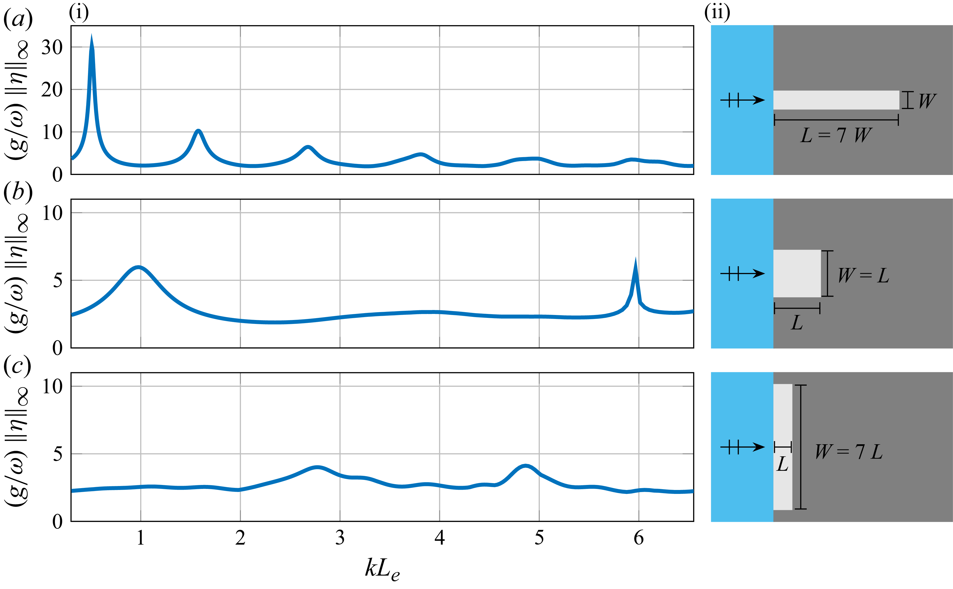
(i) Hydroelastic spectra forced by normally incident waves (
 $\alpha =0$
) for ice shelves of the same area (
 $A = 2800\,\text{km}^2$
) and thickness (
 $H=300\,\text{m}$
) and over the same constant bathymetry (
 $B=900\,\text{m}$
), but where the ice shelves have different shapes, as shown by corresponding geometries (ii), with
 $W=20\,\text{km}$
(a),
 $W\approx {}53\,\text{km}$
(b) and
 $W=140\,\text{km}$
(c).

Three different fully embedded ice shelves are studied: a narrow rectangular ice shelf, a square ice shelf and a wide rectangular ice shelf (figure 5
a ii,b ii,c ii). The ice shelves share the same horizontal span of
 $A = 2800\,\text{km}^2$
. The dimensions of the narrow ice shelf are
 $L = 140\,\text{km}$
and
 $W = 20\,\text{km}$
. The side of the square ice shelf is
 $L = W = \sqrt {A} \equiv L_{{e}} \approx 53\,\text{km}$
. The wide ice shelf has
 $L = 20\,\text{km}$
and
 $W = 140\,\text{km}$
.
Hydroelastic spectra are shown as functions of
 $kL_{{e}}$
. The results show narrow and elongated ice shelves have more distinct resonant peaks, and the fundamental mode features the maximum amplitude overall. As the ice-shelf front becomes wider, the peaks become less pronounced. Further, the maximum amplitude reduces from the narrow to the square to the wide ice shelf, whilst the response spectrum curve becomes flatter. The phenomenon of narrower embedded ice shelves experiencing larger responses is related to the harbour paradox, in which a narrower harbour opening can create larger amplitude responses within the harbour (Mei et al. Reference Mei, Stiassnie and Yue2005, Chap 5).
4.3. Incidence angle
(b) Hydroelastic spectra for a square ice shelf of side length
 $L = 53\,\text{km}$
and thickness
 $H = 300\,\text{m}$
over constant bathymetry
 $B = 900\,\text{m}$
, forced by incident waves at angles (i)
 $\alpha =0$
, (ii)
 $\alpha =\pi /6$
and (iii)
 $\alpha =\pi /4$
(as shown by insets). (a) Real and imaginary parts of ice-shelf deflection for resonances, where the colours of the bounding boxes correspond to the colours of the circles on the hydroelastic spectra, indicating the relevant resonances.

Figure 6. Long description
The image contains two main panels labeled (a) and (b), each with sub-panels. Panel (a) shows the real and imaginary parts of ice-shelf deflection for resonances, while Panel (b) displays hydroelastic spectra for a square ice shelf of side length L and thickness H over constant bathymetry, forced by incident waves at different angles. Panel (a) consists of two rows of heatmaps. The top row represents the real part (Re) of the deflection, and the bottom row represents the imaginary part (Im) of the deflection. Each column corresponds to a different resonance, with bounding boxes colored to match circles on the hydroelastic spectra in Panel (b). Panel (b) contains three sub-panels labeled (i), (ii), and (iii), each showing a line graph of the hydroelastic spectra. The x-axis is labeled kL, representing the dimensionless wavenumber, and the y-axis is labeled (g/ω) ||η||∞, representing the dimensionless amplitude of the ice-shelf deflection. Each sub-panel includes an inset showing the direction of the incident waves relative to the ice shelf. The circles on the graphs in Panel (b) correspond to the resonances shown in Panel (a), with colors matching the bounding boxes in Panel (a). The graphs illustrate how the ice-shelf deflection varies with different incident wave angles, highlighting specific resonance conditions.
Figure 6 presents hydroelastic spectra for a square shelf (side length
 $L = 53\,\text{km}$
), as a function of the non-dimensional wavenumber,
 $kL$
, for three different angles of incidence,
 $\alpha = 0$
,
 $\pi /6$
and
 $\pi /4$
. Contour plots of the real and imaginary parts of
 $\eta (x,y)$
at several resonant peaks of the spectrum are included. The angle of incidence has virtually no effect on the fundamental (lowest frequency) mode, but the remaining part of the spectrum is altered significantly in response to changes in the incidence angle. In particular, the response at some higher harmonics is enhanced for oblique incidence, e.g. the peak at
 $kL \approx 3$
is amplified as the angle increases to
 $\pi /4$
, while the deflection pattern is different at the common peak occurring at
 $kL \approx 6$
when
 $\alpha$
changes from
 $0$
to
 $\pi /6$
.
The effect of incidence angle is also studied for a semicircular ice shelf of radius
 $ L = 200 \, \text{km}$
, thickness
 $ H = 300 \, \text{m}$
and bathymetry
 $ B = 500 \, \text{m}$
(figure 7), which resembles the Larsen C Ice Shelf. Hydroelastic spectra are shown for incidence angles
 $ \alpha = 0, \pi /6, \pi /4$
. (The Sommerfeld and DtN conditions are checked for this semicircular problem and are found to be in good agreement.) The angle of incidence is again found to change the form of the amplitude spectrum and, in particular, the location of the resonant peaks. For example, when
 $ \alpha = 0$
, at
 $ kL \approx 2.8$
(period
 $ T = 1.78$
hr) the first resonant peak appears, where
 \begin{align} (g/\omega )\, \| \eta \|_{\infty }\approx 10. \end{align}
The same period corresponds to the second resonant peak when
 $ \alpha = \pi /6$
and the amplitude is reduced to
 \begin{align} (g/\omega )\, \| \eta \|_{\infty } \approx 5. \end{align}
There is no resonant peak at this period when
 $ \alpha = \pi /4$
.
Hydroelastic spectra of a semicircular ice shelf of radius
 $L = 200\,\text{km}$
and thickness
 $H = 300\,\text{m}$
over constant bathymetry
 $B = 500\,\text{m}$
(similar to the Larsen C Ice Shelf), forced by incident waves at angles (a)
 $\alpha = 0$
, (b)
 $\alpha =\pi /6$
and (c)
 $\alpha =\pi /4$
. Results are given using the DtN condition (solid blue curves) and Sommerfeld condition (broken red curves).

4.4. Grounding line geometry: ice shelves versus ice tongues
Figure 8(b) depicts two formations in Antarctica, namely the Drygalski Ice Tongue (figure 8
b i) and Amery Ice Shelf (figure 8
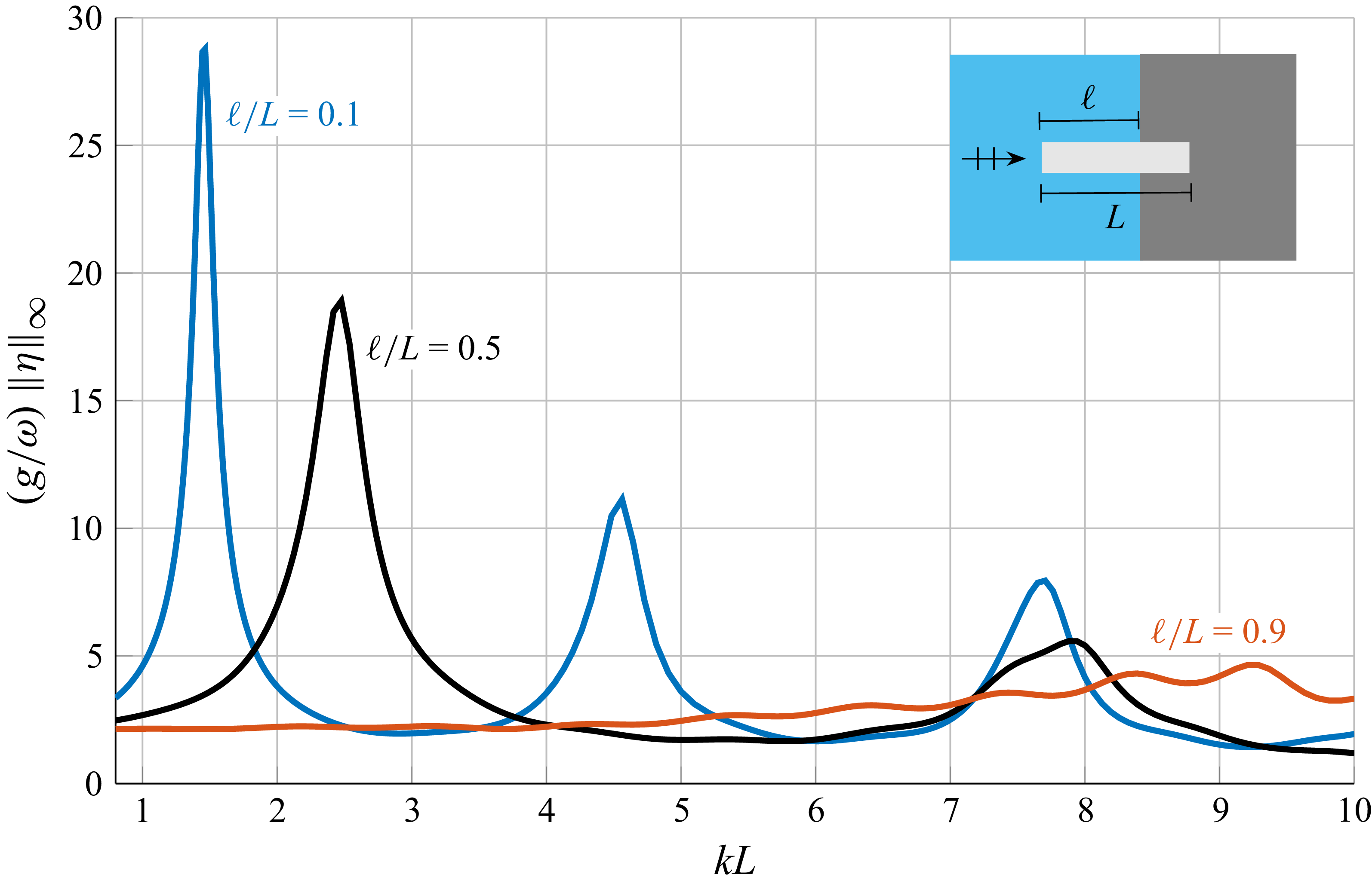
b ii). In the case of the Drygalski Ice Tongue, the grounding line (highlighted with a black line) contains only around 30 % of the ice-shelf length. In contrast, Amery Ice Shelf is fully embedded. This observation motivates a study of the influence of the proportion of the ice-shelf protrusion. Rectangular ice shelves are studied, of length
 $L=140$
km and width
 $W=20$
km (as in § 4.1), where segments of length
 $0 \leqslant l \leqslant L$
protrude into the open ocean (figure 8
a). (The ice thickness and bathymetry are
 $H = 300$
m and
 $B = 900$
m, respectively.)
Figure 9 presents hydroelastic spectra forced by normally incident waves, with
 $l/L$
values 0.1, 0.5 and 0.9, ranging from an almost fully embedded ice shelf to a mostly protruding ice tongue. As the protruding proportion,
 $l/L$
, increases, the resonant frequency peaks decrease in amplitude and shift towards higher frequencies (larger
 $kL$
values).
Figure 10 displays the velocity potential field for the three cases at wave period
 $T ={} 0.35$
hr (
 $kL\approx 7.43$
, which is close to the highest frequency resonances for
 $\ell /L=0.1$
and 0.5; figure 9). The locations of the deflection peaks and troughs change for different values of
 $l/L$
. The response of the unconfined part of the shelf has practically the same profile as the open ocean surface gravity waves. This is due to the slenderness of the chosen rectangle. Larger responses tend to occur in the region where the ice shelf is embedded.
(a) Computational domain for the scattering problem of rectangular formations with different grounding line extent. (b i) Drygalski Ice Tongue and (b ii) Amery Ice Shelf.

Figure 8. Long description
The image consists of one diagram and two satellite images. The diagram on the left side illustrates the computational domain for the scattering problem of rectangular formations with different grounding line extents. It includes various labeled sections such as Gamma R, Gamma N, Gamma g, Omega, V, and dimensions such as L, W, l, and gamma. The satellite images on the right side show two different ice shelves. The first satellite image (b i) displays the Drygalski Ice Tongue, while the second satellite image (b ii) shows the Amery Ice Shelf. Both images include grid lines and labels indicating geographical coordinates.
Hydroelastic spectra of narrow rectangular ice shelves of length
 $L$
, with constant thickness (
 $H=300\,\text{m}$
), over constant bathymetry (
 $B=900\,\text{m}$
) and in response to normally incident waves (
 $\alpha = 0$
). The protruding proportions are
 $l/L=0.1$
(blue), 0.5 (black) and 0.9 (red).

Similar to figure 4, but for ice shelves in figure 9, i.e. where the ice shelf protrudes from the coastline, with (a)
 $l/L=0.1$
, (b)
 $l/L=0.5$
and (c)
 $l/L=0.9$
, at
 $T=0.35$
hr. The perimeters of the ice shelves are indicated with black lines.

Figure 10. Long description
Panel A: Two heat maps side by side. The left heat map shows a vertical gradient with red on the left, transitioning to blue in the center, and back to red on the right. The right heat map displays a more uniform distribution with a gradient from blue to yellow. Both maps have a horizontal bar in the center with a color gradient from blue to red. The y-axis is labeled y (km) ranging from -15 to 15, and the x-axis is labeled x (km) ranging from -15 to 15. The color scale on the right ranges from -3 to 3. Panel B: Two heat maps side by side. The left heat map shows a similar vertical gradient as in Panel A, with red on the left, transitioning to blue in the center, and back to red on the right. The right heat map displays a more uniform distribution with a gradient from blue to yellow. Both maps have a horizontal bar in the center with a color gradient from blue to red. The y-axis is labeled y (km) ranging from -15 to 15, and the x-axis is labeled x (km) ranging from -15 to 15. The color scale on the right ranges from -3 to 3. Panel C: Two heat maps side by side. The left heat map shows a similar vertical gradient as in Panels A and B, with red on the left, transitioning to blue in the center, and back to red on the right. The right heat map displays a more uniform distribution with a gradient from blue to yellow. Both maps have a horizontal bar in the center with a color gradient from blue to red. The y-axis is labeled y (km) ranging from -15 to 15, and the x-axis is labeled x (km) ranging from -15 to 15. The color scale on the right ranges from -3 to 3.
5. Case study: Drygalski Ice Tongue
(a) Satellite image of Drygalski Ice Tongue and its location on map of Antarctica (red star). (b) Hydroelastic spectrum forced by normally incident waves for a model of the Drygalski Ice Tongue, including varying thickness (5.1).

Drygalski Ice Tongue model, showing normalised hydroelastic deflection (colour maps) and ocean free surface elevation (grey scale) for
 $kL \approx 7.0$
(a) and
 $kL \approx 17.3$
(b), forced by normally incident waves (
 $\alpha = 0$
). Panels (i) show the real parts and (ii) show the imaginary parts. Symmetry with respect to the horizontal axis is used to plot only the upper halves of the responses, and the lower halves are a satellite image of the modelled region.

Figure 12. Long description
Panel A: Two heat maps showing the real parts of normalized hydroelastic deflection and ocean free surface elevation for the Drygalski Ice Tongue model. The x-axis represents distance in kilometers, ranging from -200 to 0 km, and the y-axis represents distance in kilometers, ranging from -40 to 40 km. The color scale on the right indicates the real part of normalized hydroelastic deflection, with values ranging from -0.8 to 0.8. The upper half of each map shows the deflection, while the lower half is a satellite image of the modeled region. Panel (i) shows the real part of the deflection forced by normally incident waves, with a gradient of colors indicating varying deflection intensities. Panel (ii) shows a similar setup but with a different pattern of deflection. Panel B: Two heat maps showing the imaginary parts of normalized hydroelastic deflection and ocean free surface elevation for the Drygalski Ice Tongue model. The axes and color scale are the same as in Panel A. The upper half of each map shows the imaginary part of the deflection, while the lower half is a satellite image of the modeled region. Panel (i) shows the imaginary part of the deflection forced by normally incident waves, with a gradient of colors indicating varying deflection intensities. Panel (ii) shows a similar setup but with a different pattern of deflection.
The Drygalski Ice Tongue is located on the Scott Coast (Stevens et al. Reference Stevens, Lee, Fusco, Yun, Grant, Robinson and Hwang2017) and stretches for approximately 90 km into the Ross Sea (Indrigo et al. Reference Indrigo, Dow, Greenbaum and Morlighem2021). The total length of the ice tongue is approximately 140 km and the width ranges from approximately 14–24 km (the rough outline of the ice tongue with indication of the grounding line and the ice tongue front at the ocean is included in figure 11). The ice tongue thickness varies along the longitudinal axis, ranging from approximately 200 m at its snout to 2400 m at the grounding line (Indrigo et al. Reference Indrigo, Dow, Greenbaum and Morlighem2021).
A model for the Drygalski Ice Tongue is set up, where the tongue geometry is approximated by a narrow rectangle of length
 $L = 140$
km and width
 $W = 20$
km, and where the bathymetry is
 $B = 2500$
m (Indrigo et al. Reference Indrigo, Dow, Greenbaum and Morlighem2021). The protruding part of the ice shelf is set as
 $l = 98$
km, and the remaining 42 km is within the grounding line region. The thickness profile along the length of the tongue (the
 $x$
-direction), as reported in figure 2(c) by Indrigo et al. (Reference Indrigo, Dow, Greenbaum and Morlighem2021), is approximated using an exponential function
 \begin{align} H(x,y) = C_1 e^{C_2 x} \quad \text{for}\quad -98\,\text{km} \leqslant x \lt 42\,\text{km} \end{align}
with constants
 $C_1 = 1138.825$
m and
 $C_2 = 1.775 \boldsymbol{\times }10^{-5}\,\text{m}^{-1}$
. Mild variations of the thickness along the
 $y$
-direction are neglected.
The hydroelastic spectrum for normally incident waves (figure 11) reveals a resonant peak at
 $kL \approx 6$
, which corresponds to a period of
 $T = 0.22$
hr (a possible tsunami wave period), where the flexure reaches values
 ${\gt } 5$
. Figure 12 shows the deflection fields (normalised by the maximum displacement for simplicity of presentation) at the resonant period (
 $T = 0.22$
hr; figure 12
a) and at
 $T = 0.09$
hr (
 $kL \approx 17.3$
), which is representative of the higher frequency responses in the range shown. In both cases, the deflection at the protruding part of the tongue follows the open ocean free surface elevation. The ice within the grounding line border exhibits a monopole-type shape for
 $T = 0.22$
hr and a dipole-type shape for
 $T = 0.09$
hr.
6. Conclusions
A solution method has been presented for a water wave scattering problem involving the hydroelastic response of an ice shelf embedded along a flat coastline to incident waves from the open ocean. The proposed approach combines a finite element method (FEM), where non-conforming hydroelastic finite element triangles are used for the high-order ice-shelf–water cavity region, and a DtN mapping to apply the radiation condition in the open ocean. The solution is efficient enough to study the hydroelastic response spectra of the ice shelf to incident wave forcing over the broad wavenumber range. Numerical results were used to conduct a novel study on how the ice-shelf response is influenced by the incident wave angle, the ice-shelf shape and the proportion of the ice-shelf boundary attached to land. In all cases, it was shown that significant effects in the response spectra could be produced. The findings indicate the potential importance of models that include non-uniform motions in the spanwise direction. Results for a model of the Drygalski Ice Tongue were presented, which identified a resonant peak in the response spectra over the studied wavenumber range that indicate that if the Drygalski was excited by tsunami waves then it could experience large flexure.
The numerical method presented could be extended to accommodate a model in which the coastline surrounding the ice shelf is not straight, which may influence ice-shelf flexure, e.g. in cases when it is in a bay (such as the Amery Ice Shelf, figure 1 a). In particular, the reflected wave field (2.13) would need to be modified, as in Steward & Panchang (Reference Steward and Panchang2001). Similarly, the varying bathymetry could be extended beyond the ice-shelf/cavity region, although this would require modifications of the DtN condition. The method could also be extended to model partially absorbing coastlines, i.e. changing from a Neumann to a Robin boundary condition (Isaacson & Qu Reference Isaacson and Qu1990).
The shallow-water approximation (2.9) is unlikely to be accurate for the incident ocean swell that have been heavily implicated in major ice-shelf calving events (Massom et al. Reference Massom, Scambos, Bennetts, Reid, Squire and Stammerjohn2018; Teder et al. Reference Teder, Bennetts, Reid, Massom, Pitt, Scambos and Fraser2025), as swell often have wave periods
 ${\lt } 15$
s. Replacing the shallow-water approximation with the so-called single-mode approximation (Bennetts et al. Reference Bennetts, Biggs and Porter2007) would extend the validity of the model into the swell regime (Bennetts & Meylan Reference Bennetts and Meylan2021) and maintain the shallow-water structure of the governing equations, such that the solution method could be adapted to it in a straightforward manner. However, incorporating the bending moments applied by incident swell on shelf fronts (Bennetts et al. Reference Bennetts, Williams and Porter2024a
; Bennetts & Liang Reference Bennetts and Liang2026) in the model would require modifications to the method. Further, Chen et al. (Reference Chen, Bromirski, Gerstoft, Stephen, Wiens, Aster and Nyblade2018) observed that flexural waves forced by swell attenuate with distance travelled into ice shelves. This implies viscosity in the ice-shelf response should be considered in the swell regime, which could be incorporated into the model used in the presented study using, e.g. the viscoelastic model for ice-shelf flexure proposed by MacAyeal et al. (Reference MacAyeal, Sergienko and Banwell2015).
In conclusion, we have contributed a solution method for a model of hydroelastic flexure of ice shelves excited by long ocean waves, where variations in both horizontal dimensions are incorporated and the ice shelf is of arbitrary shape, including varying thickness. The method is efficient enough to study the ice-shelf response spectra and identify resonances. Moreover, we have contributed new understanding of the dependence of the ice-shelf response to incident waves on parameters that exist due to the second spatial dimension. Our study sets the computational basis for understanding which Antarctic ice shelves are most susceptible to impacts by long ocean waves.
Acknowledgements
The authors thank the Isaac Newton Institute for Mathematical Sciences, Cambridge, for its support and hospitality during the programme Multiple Wave Scattering, where this work was initiated.
Funding
This work was supported by the Isaac Newton Institute for Mathematical Sciences, Cambridge, through EPSRC grant no. EP/R014604/1. L.G.B. and M.H.M. were supported by the Australian Research Council under grants FT190100404, SR200100008, DP240100325 and DP240102104.
Declaration of interests
The authors declare no competing interests.
Data availability statement
The data for the study is freely available, see Papathanasiou et al. (Reference Papathanasiou, Bennetts and Meylan2026).
Appendix A. Neglect of Coriolis effects
Assuming an average southern latitude of
 $80^\circ$
, the Coriolis frequency is given by
 \begin{align} f = 2\Omega _e \sin (80^\circ ), \end{align}
where
 $\Omega _e$
is the angular velocity of Earth’s rotation. This implies a Coriolis period of approximately
 \begin{align} T_f \approx {12}\mathrm{h}. \end{align}
The maximum wave period in the band of interest is
 $T_m \approx {4}\mathrm{h}$
, and the corresponding Rossby number is
 \begin{align} \mathrm{Ro} = \frac {T_f}{T_m} \approx 3. \end{align}
This Rossby number indicates that the Coriolis force effect is weak compared with other restoring forces (such as gravity and acceleration) in the waveband of interest (15 s to 4 hr). Therefore, Coriolis effects are not included in the study.
Appendix B. Derivation and implementation of the DtN condition
The incident and reflected wave, using the Jacobi–Anger expansion, can be written as
 \begin{align} \phi _I = e^{ikr(\cos \theta \cos \alpha + \sin \theta \sin \alpha )} = e^{ikr\cos (\alpha - \theta )} = \sum _{n=-\infty }^{\infty } i^n J_n(kr) e^{in(\alpha - \theta )}, \end{align}
and
 \begin{align} \phi _R = e^{ikr(-\cos \theta \cos \alpha + \sin \theta \sin \alpha )} = e^{-ikr\cos (\alpha + \theta )} = \sum _{n=-\infty }^{\infty } (-1)^n i^n J_n(kr) e^{in(\alpha + \theta )}, \end{align}
where
 $ J_n(kr)$
is the Bessel function of the first kind and order
 $ n$
. Then,
 \begin{align} \phi _I + \phi _R = \sum _{n=-\infty }^{\infty } i^n e^{in\alpha } J_n(kr) \varLambda _n(\theta ), \end{align}
where
 \begin{align} \varLambda _n(\theta ) = \begin{cases} 2 \cos (n\theta ), & \text{for } n \text{ even}, \\ -2i \sin (n\theta ), & \text{for } n \text{ odd}. \end{cases} \end{align}
Since
 $ \partial \phi / \partial \theta = 0$
at
 $ \theta = \pi /2, 3\pi /2$
, and using
 $ J_{-n}(kr) = (-1)^n J_n(kr)$
, it follows that
 \begin{align} \phi _I + \phi _R = \sum _{n=0,2,4,\ldots }^{\infty } A_n \frac {J_n(kr)}{J_n(kR)} \cos (n\theta ) + \sum _{n=1,3,5,\ldots }^{\infty } B_n \frac {J_n(kr)}{J_n(kR)} \sin (n\theta ), \end{align}
with
 \begin{align} A_0 = 2 J_0(kR), \quad A_n = 4 i^n \cos (n\alpha ) J_n(kR), \quad n = 2, 4, 6, \ldots\nonumber\\[-30pt] \end{align}
 \begin{align} \text{and}\quad B_n = 4 i^n \sin (n\alpha ) J_n(kR), \quad n = 1, 3, 5, \ldots . \end{align}
The scattering potential
 $ \phi _s$
is now expanded as
 \begin{align} \phi _s = \sum _{n=0,2,4,\ldots }^{\infty } C_n \frac {H_n^{(1)}(kr)}{H_n^{(1)}(kR)} \cos (n\theta ) + \sum _{n=1,3,5,\ldots }^{\infty } D_n \frac {H_n^{(1)}(kr)}{H_n^{(1)}(kR)} \sin (n\theta ), \end{align}
where
 $ H_n^{(1)}(kr)$
is the Hankel function of the first kind and order
 $ n$
. At
 $ r = R$
, we have
 \begin{align} \phi (R, \theta ) = \phi _I(\theta ) + \phi _R(\theta ) + \phi _s(\theta ) &= \sum _{n=0,2,4,\ldots }^{\infty } (A_n + C_n) \cos (n\theta ) \nonumber\\& + \sum _{n=1,3,5,\ldots }^{\infty } (B_n + D_n) \sin (n\theta ). \end{align}
Using the orthogonality conditions for trigonometric functions, the coefficients are
 \begin{align} A_0 + C_0 = \frac {1}{\pi } \int _{\pi /2}^{3\pi /2} \phi (\vartheta ) {\rm d}\vartheta = I_0, \end{align}
 \begin{align} A_n + C_n = \frac {2}{\pi } \int _{\pi /2}^{3\pi /2} \cos (n\vartheta ) \phi (\vartheta ) {\rm d}\vartheta = I_n, \quad n = 2, 4, 6, \ldots \end{align}
 \begin{align} \text{and}\quad B_n + D_n = \frac {2}{\pi } \int _{\pi /2}^{3\pi /2} \sin (n\vartheta ) \phi (\vartheta ) {\rm d}\vartheta = K_n, \quad n = 1, 3, 5, \ldots ~. \end{align}
Then, at
 $ r = R$
, the radial derivative is
 \begin{align} \left . \frac {\partial \phi }{\partial r} \right |_{r=R} & = \sum _{n=0,2,4,\ldots }^{\infty } \left [ \frac {A_n W_n}{J_n(kR) H_n^{(1)}(kR)} + I_n \frac {H_n^{(1)'}(kR)}{H_n^{(1)}(kR)} \right ] \cos (n\theta ) \end{align}
 \begin{align} & \, + \sum _{n=1,3,5,\ldots }^{\infty } \left [ \frac {B_n W_n}{J_n(kR) H_n^{(1)}(kR)} + K_n \frac {H_n^{(1)'}(kR)}{H_n^{(1)}(kR)} \right ] \sin (n\theta ). \end{align}
The Wronskian
 $ W_n$
is
 \begin{align} W_n = J_n'(kR) H_n^{(1)}(kR) - H_n^{(1)'}(kR) J_n(kR) = -\frac {2i}{\pi R}. \end{align}
The normal derivative at
 $ r = R$
then has the form
 \begin{align} \left . \frac {\partial \phi }{\partial r} \right |_{r=R} = f(R, \theta ) + \int _{\pi /2}^{3\pi /2} G(R, \theta , \vartheta ) \phi (R, \vartheta ) {\rm d}\vartheta , \end{align}
where the function
 $ f(R, \theta )$
is
 \begin{align} f(R, \theta ) = \sum _{n=0,2,4,\ldots }^{\infty } \frac {A_n W_n \cos (n\theta )}{J_n(kR) H_n^{(1)}(kR)} + \sum _{n=1,3,5,\ldots }^{\infty } \frac {B_n W_n \sin (n\theta )}{J_n(kR) H_n^{(1)}(kR)}, \end{align}
and the kernel function is
 \begin{align} G(R, \theta , \vartheta ) = \frac {M_0}{\pi } + \frac {2}{\pi } \sum _{n=2,4,6,\ldots }^{\infty } M_n \cos (n\theta ) \cos (n\vartheta ) + \frac {2}{\pi } \sum _{n=1,3,5,\ldots }^{\infty } M_n \sin (n\theta ) \sin (n\vartheta ), \end{align}
with
 \begin{align} M_n = \frac {H_n^{(1)'}(kR)}{H_n^{(1)}(kR)} = \frac {n}{R} - k \frac {H_{n+1}^{(1)}(kR)}{H_n^{(1)}(kR)}. \end{align}
When the DtN condition is applied on
 $ \varGamma _R$
, the following integrals need to be computed:
 \begin{align} I_1 = \int _{\varGamma _R} B \bar {w}^h \left ( \int _{\pi /2}^{3\pi /2} G(R, \theta , \vartheta ) \phi (R, \vartheta ) \, {\rm d}\vartheta \right ) {\rm d}\varGamma \quad \text{and}\quad I_2 = \int _{\varGamma _R} B \bar {w}^h f(R, \theta ) \, {\rm d}\varGamma . \end{align}
These integrals are computed numerically in the MATLAB code used for this study. The accuracy of the numerical integration matches the accuracy of the finite element formulation, so that the overall convergence rate is not affected. In the following,
 $ \varGamma _R$
is assumed to be composed of
 $ N$
element edges for elements
 $ e_j$
,
 $ j = 1, 2, \ldots , N$
. Starting with the second integral and denoting each term of the series expansion of
 $ f$
as
 $ f_n$
, it is
 \begin{align} I_2 \approx \sum _{n=0}^{\infty } \sum _{j=1}^{N} \int _{e_j} B \bar {w} f_n(R, \theta ) \, {\rm d}\varGamma . \end{align}
For each element on
 $ \varGamma _R$
, the forcing vector has two non-zero terms, which are approximated using the midpoint rule and the resulting linear Lagrange shape functions on the element edge (
 $ \theta _j = \arccos (x_j / R)$
is the angle corresponding to the midpoint of the
 $ e_j$
element edge, and
 $ h_j$
is the element edge length) as
 \begin{align} f_1 = f_2 \approx \frac {B}{2} h_j \sum _{n=0}^{\infty } f_n(R, \theta _j). \end{align}
For the first integral
 $ I_1$
, the inner part is considered first. It is
 \begin{align} \int _{\pi /2}^{3\pi /2} G(R, \theta , \vartheta ) \phi (R, \vartheta ) \, {\rm d}\vartheta &= \sum _{n=0}^{\infty } \sum _{i=1}^{N} \int _{e_i} G_n(R, \theta , \vartheta ) \phi (R, \vartheta ) \, {\rm d}\vartheta \nonumber\\&\approx \frac {1}{R} \sum _{n=0}^{\infty } \sum _{i=1}^{N} G_n(R, \theta , \vartheta _i) \phi (R, \vartheta _i) h_i. \end{align}
However, the value
 $ \phi (R, \vartheta _i)$
is not a nodal degree of freedom. At the same order of approximation with the elements used,
 \begin{align} \phi (R, \vartheta _i) = \frac {\phi (R, \vartheta _{A_{1i}}) + \phi (R, \vartheta _{A_{2i}})}{2} = \frac {\phi _{A_{1i}} + \phi _{A_{2i}}}{2} \end{align}
for an element with nodes on
 $ \varGamma _R$
denoted
 $ A_1, A_2$
. Then, handling the outer integral as in the case of
 $ I_2$
, the local element contributions from the application of the DtN condition to the stiffness matrix and force vector are (for element
 $ e_j$
on
 $ \varGamma _R$
)
 \begin{align} I_1 \big |_{e_j} \approx \frac {B}{4R} \sum _{i=1}^{N} \sum _{n=0}^{\infty } G_n(R, \theta _j, \vartheta _i) h_i h_j \begin{bmatrix} 1 & 1 \\ 1 & 1 \end{bmatrix} \begin{bmatrix} \phi _{A_{1i}} \\ \phi _{A_{2i}} \end{bmatrix}, \end{align}
 \begin{align} I_2 \big |_{e_j} \approx \frac {B}{2} \sum _{n=0}^{\infty } f_n(R, \theta _j) h_j \begin{bmatrix} 1 \\ 1 \end{bmatrix}. \end{align}
The implementation is done by truncating the infinite series over
 $ n$
to a term
 $ N_n$
and assembling the element contributions over
 $ \varGamma _R$
to the global stiffness matrix and force vector, respectively.
Appendix C. Validation for the harbour problem
The code used in the study is modified for use on the degenerate problem of harbour excitation by long waves, in which the ice shelf (Kirchoff–Love plate) is removed from
 $\Omega$
, which allows for verification against results from the existing literature. The case of a circular harbour of radius
 $a$
was chosen, with a narrow opening to the surrounding ocean. Bigg & Tuck (Reference Bigg and Tuck1982) solved the problem using the method of matched asymptotoic expansions and gave results for the modulus of the velocity potential at three locations in the harbour (A, B and C in figure 13
a) in their figure 9. The analogous results generated from the code used for the present study (using the DtN condition with
 $R=3a$
and
 $N_{{el}}=14,464$
elements) agree well with the results from Bigg & Tuck (Reference Bigg and Tuck1982) (figure 13
b).
The circular harbour geometry with a small opening to the surrounding ocean, the mesh used (blue lines) and the sampled locations A, B and C (a). The response spectra in terms of the modulus of the velocity potential versus non-dimensional wavenumber
 $ka$
at locations A, B and C (b), using the code developed in this study (FEM with the DtN condition; solid curves) and by Bigg & Tuck (Reference Bigg and Tuck1982) (broken curves).


 H(x,y)
 B(x,y)

 Ω
 V

 R=2L
 n=10
 Nel=11,200
 R=20L
 Nel=404,480
 Td,j
 j=1,2,3
 L=140
 W=20
 H=300m
 B=900m
 Td,j
 j=1
 j=2
 j=3

 Φ(x,y)
 x>0
 φ(x,y)
 x<0
 T=Td,1=1.98
 Td,2=0.66
 Td,3=0.40
 Im(Φ)≈30
 α=0
 A=2800km2
 H=300m
 B=900m
 W=20km
 W≈53km
 W=140km

 L=53km
 H=300m
 B=900m
 α=0
 α=π/6
 α=π/4

 L=200km
 H=300m
 B=500m
 α=0
 α=π/6
 α=π/4

 L
 H=300m
 B=900m
 α=0
 l/L=0.1

 l/L=0.1
 l/L=0.5
 l/L=0.9
 T=0.35


 kL≈7.0
 kL≈17.3
 α=0

 ka

 Open access

