





1. Introduction
Aquatic canopies in fluvial systems alter the local flow dynamics and create coherent structures in their wake, which affect transport and mixing processes (Nepf Reference Nepf2012). These canopies, found in the form of porous patches containing vegetation, occupy various parts of river channels and floodplains (Carr et al. Reference Carr, Duthie and Taylor1997; Sukhodolov & Sukhodolova Reference Sukhodolov and Sukhodolova2010). They serve as ecological engineers (Jones et al. Reference Jones, Sharitz, Dixon, Segal and Schneider1994; Costanza et al. Reference Costanza1997; Corenblit & Steiger Reference Corenblit and Steiger2009; Gurnell Reference Gurnell2014) and create regions with enriched nutrients, enhanced light penetration and increased plant productivity (Webster & Benfield Reference Webster and Benfield1986; Wilcock et al. Reference Wilcock, Champion, Nagels and Croker1999; Horppila & Nurminen Reference Horppila and Nurminen2003; Schultz et al. Reference Schultz, Kozerski, Pluntke and Rinke2003; Schoelynck et al. Reference Schoelynck, De Groote, Bal, Vandenbruwaene, Meire and Temmerman2012; Camporeale et al. Reference Camporeale, Perucca, Ridolfi and Gurnell2013). Vegetation canopies also affect channel morphology at the patch scale (Carroppi et al. Reference Caroppi, Gualtieri, Fontana and Giugni2020; Zhang et al. Reference Zhang, Duan, Yan and Stocchino2023), enhance biodiversity and water quality in fluvial systems (e.g. by trapping suspended particles) and provide habitats to fish, birds, insects and larvae by protecting them from predators (Schultz et al. Reference Schultz, Kozerski, Pluntke and Rinke2003; Beechie et al. Reference Beechie, Liermann, Pollock, Baker and Davies2006).
Vegetation canopies reduce river transport capacity due to increased plant-induced drag (Tal & Paola Reference Tal and Paola2007; Plew et al. Reference Plew, Cooper and Callaghan2008; Tanino & Nepf Reference Tanino and Nepf2008), create flow acceleration zones which induce bed erosion and nutrient limitation (i.e. negative feedback for patch growth) and generate substantial turbulence (Ghisalberti & Nepf Reference Ghisalberti and Nepf2002; Righetti & Armanini Reference Righetti and Armanini2002; Liu et al. Reference Liu, Diplas, Fairbanks and Hodges2008; Zong & Nepf Reference Zong and Nepf2012; Chang et al. Reference Chang, Constantinescu and Tsai2017; Koken & Constantinescu Reference Kirkil and Constantinescu2020, Reference Koken and Constantinescu2023). Nutrient transport within canopies and plant nutrient uptake depend on the vertical momentum, secondary flow and turbulence intensity within the canopy. Turbulence, especially that generated near the canopy front and its sides, inhibits deposition and resuspension, leading to bed scouring (Souliotis & Prinos Reference Souliotis and Prinos2010; Sukhodolov & Sukhodolova Reference Sukhodolov and Sukhodolova2014; Yang et al. Reference Yang, Chung and Nepf.2016; Zhang & Nepf Reference Zhang and Nepf2025). Inside the canopy, sediment deposition and nutrient accumulation are enhanced, while sediment erosion is reduced (Gurnell et al. Reference Gurnell, Tockner, Edwards and Petts2005; Bouma et al. Reference Bouma, Van Duren, Temmerman, Claverie, Blanco-Garcia, Ysebaert and Herman2007; van Wesenbeck et al. Reference Van Wesenbeeck, Van De Koppel, MJ Herman and J. Bouma2008; Schoelynck et al. Reference Schoelynck, De Groote, Bal, Vandenbruwaene, Meire and Temmerman2012; Follett & Nepf Reference Follett and Nepf2012; Liu & Nepf Reference Liu and Nepf2016; Liu et al. Reference Liu, Hu, Lei and Nepf2018; Zhang & Nepf Reference Zhang and Nepf2025). Canopy velocity regulates fine sediment retention and carbon sequestration (Dahl et al. Reference Dahl, Infantes, Clevesjö, Linderholm, Björk and Gullström2018; Lei & Nepf Reference Lei and Nepf2021). The steady wake region at the back of the canopy is characterised by small velocities and weak turbulence, thus deposition is enhanced (Chen et al. Reference Chen, Ortiz, Zong and Nepf2012). Its length increases with the magnitude of the bleeding flow at the trailing edge of the canopy (Chang & Constantinescu Reference Chang and Constantinescu2015).
Most isolated, three-dimensional (3-D) canopies have shapes close to rectangular or circular (Chen et al. Reference Chen, Ortiz, Zong and Nepf2012). In natural streams, isolated canopies are common during initial stages of seasonal vegetation growth. Beyond vegetated open channel flows, understanding the physics of canopy flows and the influence of surface-mounted permeable obstacles on surrounding flow is relevant for a range of other applications (Lai et al. Reference Lai, Katul, Oren, Ellsworth and Schäfer2000; Chen et al. Reference Chen, Ortiz, Zong and Nepf2012; Hamed et al. Reference Hamed, Sadowski, Nepf and Chamorro2017). For example, quantifying turbulent fluxes like water vapour and CO2 is very important for forest canopies. Other types of relevant applications involve the deployment of artificial porous structures (e.g. bamboo arrays) used to facilitate vegetation colonisation, mitigate erosion and dissipate wave energy in coastal environments (Siemes et al. Reference Siemes, Borsje, Daggenvoorde and Hulscher2020; Siegersma et al. Reference Siegersma, Willemsen, Horstman, Hu and Borsje2023).
Research on the flow around vegetation canopies has mainly focused on idealised scenarios. Several studies (e.g. White and Nepf Reference White and Nepf2008; Tanino & Nepf Reference Tanino and Nepf2008; Rominger et al. Reference Rominger, Lightbody and Nepf2010; Zong & Nepf Reference Zong and Nepf2010, Reference Zong and Nepf2011, Reference Zong and Nepf2012; Rominger & Nepf Reference Rominger and Nepf2011; Chen et al. Reference Chen, Ortiz, Zong and Nepf2012; Kim et al. 2015; Chang et al. Reference Chang, Constantinescu and Tsai2017, Reference Chang, Constantinescu and Tsai2024; Koken & Constantinescu Reference Koken and Constantinescu2020; Zhang et al. Reference Zhang, Duan, Yan and Stocchino2023; Zhang & Nepf Reference Zhang and Nepf2025) investigated the flow physics of isolated canopies with uniform porosity and rigid circular elements as a surrogate for rigid plant stems (e.g. reeds, mangroves). Plant flexibility was neglected in these studies that involved mainly circular or rectangular canopies placed at the centre of the channel, or long rectangular canopies situated at one of the channel banks. Liu et al. (Reference Liu, Hu, Lei and Nepf2018), Chang et al. (Reference Chang, Constantinescu and Tsai2020), Lei & Nepf (Reference Lei and Nepf2021) and Koken & Constantinescu (Reference Koken and Constantinescu2023) studied the wake structure and the shear layers forming on the sides of long rigid canopies, while Zhang et al. (Reference Zhang, Duan, Yan and Stocchino2023) focused on the wake structure past rectangular canopies with varying aspect ratio. Rominger & Nepf (Reference Rominger and Nepf2011) and Kim et al. (2015) found that the flow inside the array attains equilibrium (i.e. becomes independent of the distance to the leading edge of the array) for patches with a sufficiently high aspect ratio. Rominger & Nepf (Reference Rominger and Nepf2011) proposed a formula to estimate the interior adjustment length, L a , defined as the streamwise distance from the leading edge where the flow inside the array reaches equilibrium. This length decreases with increasing array density and increased bluffness of the array’s elements. Arrays with a length smaller than L a will be characterised by a larger bleeding velocity (i.e. velocity at the trailing edge of the array). White & Nepf (Reference White and Nepf2007), Zong & Nepf (Reference Zong and Nepf2012) and Chang & Constantinescu (Reference Chang and Constantinescu2015) discuss the critical values of the geometrical parameters characterising the array’s element density for the anti-symmetric vortex shedding mode to be dominant in the array’s wake. This mode is associated with the formation of counter-rotating wake billows in the region where the separated shear layers forming on the two sides of the array interact (i.e. end of steady wake region). In all these studies, the canopy region is formed by a rectangular or circular array of identical rigid cylinders placed in a regular, or slightly randomised, arrangement such that the porosity or, equivalently, the solid volume fraction (SVF) of the canopy can be considered constant.
Numerical simulations that resolve the flow around the individual canopy elements eliminate the need for empirical terms to account for flow deceleration and turbulence generation within the canopy. For instance, Huai et al. (Reference Huai, Xue and Qian2015), Chang et al. (Reference Chang, Jiang, Constantinescu and Jung2017, Reference Chang, Constantinescu and Tsai2020, Reference Chang, Constantinescu and Tsai2024), Liu et al. (Reference Liu, Huai, Ji and Han2021), Koken & Constantinescu (Reference Koken and Constantinescu2020, Reference Koken and Constantinescu2023) and Yuksel-Ozan et al. (Reference Yuksel-Ozan, Chang, Gunes and Constantinescu2026) analysed flow around and inside emerged and submerged arrays of rigid cylinders positioned near, or away from, the sidewalls of an open channel. Such studies conducted using eddy resolving techniques based on the large eddy simulation (LES) approach provided detailed data on the bed shear stresses within and outside the array, the forces on the individual cylinders (i.e. canopy elements/stems), the velocity and turbulent kinetic energy (TKE) profiles inside the array, and momentum fluxes on the boundary surfaces of the array/canopy. Moreover, these simulations were used to quantitatively characterise complex 3-D effects (e.g. downflow close to the upstream face of the canopy that partially penetrates inside the array, dynamics of the horseshoe vortices forming around the upstream face of the array), the vertical transport inside the shear layers forming on the lateral sides of the array and secondary flow patterns (e.g. upwelling and downwelling motions) within the array and in its wake. Such data are challenging to obtain through flume experiments. This information is crucial for understanding the overall flow structure, the role of coherent structures in driving erosion and deposition inside and around the array and canopy-induced drag. Even though natural vegetation in rivers is generally characterised by a certain degree of flexibility, a fundamental understanding of the flow physics is needed for the limiting case of rigid vegetation with respect to which the effect of plant flexibility can be quantified in a systematic way. For example, this approach was followed by Chen & Li (Reference Chen and Li2025) for an isolated circular plant stem.
Another fundamental problem related to theoretical and numerical modelling of flow past finite-size, porous canopies that do not resolve the flow past the individual elements/stems is the specification of the bulk drag coefficient for the elements forming the array/canopy, C
da
. For high Reynolds number flows, the bulk drag coefficient is usually reported as a single value for the entire canopy, assuming each element experiences a force equal to the total canopy streamwise drag force divided by the number of elements. The choice of the appropriate velocity scale for C
da
is also important. For fully porous channels, the channel-averaged, in-canopy (streamwise) velocity,
 $\overline{\overline{U}}$
, is commonly used. For finite-size canopies, the incoming bulk channel velocity, U
0, or the double-averaged (i.e. over time, canopy height, H, and canopy width, D) in-canopy velocity,
 $\overline{\overline{U}}$
(x), are commonly used. The latter choice looks more physical despite the very non-uniform (streamwise) distribution of the in-canopy mean streamwise velocities inside most 3-D canopies (Koken & Constantinescu Reference Koken and Constantinescu2020, Reference Koken and Constantinescu2023). The main geometrical parameters affecting C
da
for canopies with uniform, or close to uniform, porosity are the SVF, which is defined as the ratio between the volume occupied by the canopy elements/stems and the canopy volume, the non-dimensional frontal area per unit volume of the canopy,
 $\textit{aD}$
, the shape of the canopy elements and relative size,
 $d/D$
, of the canopy elements, where d is the width of the elements. Some studies found that C
da
increases with
 $\textit{SVF}$
(Tanino & Nepf Reference Tanino and Nepf2008; Cheng & Nguyen Reference Cheng and Nguyen2011), while others found the opposite (Nepf Reference Nepf1999; Lee et al. Reference Lee, Roig, Jenter and Visser2004). The sheltering effect from neighbouring elements and their arrangement contribute to these variations. Moreover, Koken & Constantinescu (Reference Koken and Constantinescu2020, Reference Koken and Constantinescu2023) noted differences between the (width-averaged) drag coefficients for the individual canopy elements
 ${C}_{d}^{\prime}$
defined with d, H and the local value of
 $\overline{\overline{U}}$
(x) inside a rectangular, emerged, sidewall canopy containing circular rigid cylinders and those inferred from experiments in which the canopy occupies the whole channel (i.e. fully porous channel where
 $\overline{\overline{U}}$
is characterised by a unique value) despite the same values of the stem Reynolds number
 $\overline{\textit{Re}_{d}} = \overline{\overline{U}}d/$
ν (ν is the kinematic viscosity),
 $\textit{SVF}$
and/or
 $\textit{aD}$
. Experimental studies of 3-D canopy flows do not provide measurements of the drag forces acting on the canopy elements which are needed to estimate
 ${C}_{d}^{\prime}$
(x). However, such information is important to understand the behaviour of vegetated canopies (Sarsu et al. Reference Sarsu, Doppler, Jerome, Riviere and Lance2016) and to correctly specify the drag coefficient in analytical models and in empirical models used to predict different variables for finite-size canopy flows. Finally, the flow blockage parameter for 3-D canopies of width D is C
da
 $\textit{aD}$
/2. This is a main variable in many empirical models used to predict quantities of engineering interest for canopy flows. Lack of quantitative data on how C
da
varies with the main geometrical parameters of the array is the main reason why very rough approximations are used to prescribe this variable. For example, for arrays containing circular cylinders and for relatively high cylinder Reynolds numbers (i.e. Re
d
= U
0
d/ν > >100), C
da
is generally assumed to be equal to unity (e.g. see Zhang et al. Reference Zhang, Duan, Yan and Stocchino2023).
Sketch of the computational domain showing the position of the square array of width D inside the straight, flat-bed open channel of width W and length 20.5D. The array contains either circular or rectangular cylinders of width d. The channel flow depth, H, is equal to the array height, h c . The channel bulk velocity is U 0.

Figure 1. Long description
A sketch of the computational domain illustrating the position of a square array of width D inside a straight, flat-bed open channel of width W and length 20.5D. The array contains either circular or rectangular cylinders of width d. The channel flow depth, H, is equal to the array height, hc. The channel bulk velocity is U0. The diagram includes labels for the x and y axes, with specific positions marked along the x-axis at 0, 2.5D, 3.5D, and 20.5D. The y-axis is labeled at -W/2, 0, and W/2. The array is shown at an angle of 70 degrees, and a magnified view of the array is provided within a red dashed box.
The geometrical set-up of the present study (figure 1) is similar to that used in the experiments of White & Nepf (Reference White and Nepf2007) and Zhang et al. (Reference Zhang, Duan, Yan and Stocchino2023) focusing on rectangular arrays containing emerged circular rigid cylinders placed at the centre of an open channel. The present study considers an in-stream square array of size D*D containing close to uniformly distributed identical elements (circular or rectangular rigid cylinders of same cross-sectional area) placed in a channel of depth H with fully developed turbulent incoming flow (Re
D
= U
0
D/ν = 40 000, Re
H
= U
0
D/ν = 14 000). The main geometrical parameters that affect the flow around and through the array and the total drag acting on the array are
 $\textit{SVF}$
, aD, d/D and the shape of the cylinders. Additionally, the ratio between the width of the channel and the array’s width,
 $W/D$
, can also affect the flow and drag forces due to blockage effects in a width-limited environment, a common case for 3-D vegetation canopies in natural streams and especially for canopy experiments performed in a laboratory flume. For elements of same width, d, varying
 $\textit{SVF}$
or
 $\textit{aD}$
is equivalent, but this is not true if
 $d/D$
or d/s (s is the average distance between neighbouring cylinders) are not the same in the simulations/experiments. As such, the main objective of the paper is to understand how the main geometrical parameters of the array (i.e.
 $\textit{SVF}$
, aD, d/D, cylinder shape) and the blockage ratio,
 $W/D$
, affect:
-
(i) The formation and coherence of the horseshoe vortices forming around the upstream face of the array and their interactions with the coherent structures inside the wake.
-
(ii) The wake structure and, in particular, the anti-symmetric wake shedding mode, the size and position of the mean-flow recirculation bubbles forming inside the near wake, the lengths of the steady wake and total wake regions and the formation of streamwise-oriented vortices inside the near wake.
-
(iii) The streamwise distributions of the double-averaged mean streamwise velocity,
 $\overline{\overline{U}}$
, and TKE,
$\overline{\overline{k}}$
, and the bleeding flow velocity at the back of the array, U
b.
-
(iv) The bed shear stress distributions and the capacity of the flow to induce sediment entrainment inside and around the array in the case of a loose bed.
-
(v) The streamwise variation of the mean (spanwise-averaged) non-dimensional drag forces acting on the cylinders and cylinder drag coefficient,
${C}_{d}^{\prime}$
, as well as the variation of
${C}_{d}^{\prime}$
with
$\overline{\textit{Re}_{d}}$
. -
(vi) The total non-dimensional drag force acting on the array, C D , and the mean cylinder drag coefficient over the part of the array where the quadratic drag regime is observed,
$\overline{{C}_{d}^{\prime}}$
.


Section 2 provides some information on the numerical method, boundary conditions and the main flow and geometrical parameters of the test cases. Section 3 focuses on the effects of the main geometrical parameters describing the array and of the blockage ratio on the horseshoe vortex system forming around the upstream face of the array, the double-averaged velocity and TKE inside the array. Section 4 discusses how the same geometrical parameters affect the coherent structures forming inside the array’s shear layers and wake, the mean-flow structure inside the near-wake region and its spectral content. Section 5 focuses of the effect of the main geometrical parameters on the distributions of the mean bed shear stress and the root mean square of the bed shear stress and on the capacity of the flow to induce sediment erosion outside and inside the array. Section 6 focuses on the drag forces acting on the cylinders forming the array and the eventual presence of the linear drag regime inside the downstream part of the array. It also provides information on the effect of the main geometrical parameters on the mean cylinder drag coefficient over the part of the array where the quadratic drag regime is present, which is the main parameter that needs to be provided in numerical models that do not resolve the flow past the array’s elements and use an added drag terms in the governing equations, as well in theoretical models of canopy flows. Section 7 summarises the main results and provides some conclusions.
2. Description of the computations
2.1. Test cases
Simulations were conducted with a square emerged array of width D = 0.4 m placed in an open channel L = 20.5D long (figure 1) with a bulk incoming flow velocity U
0 = 0.1
 $\textrm{m}\, \textrm{s}^{-1}$
and a water depth H = 0.14 m (i.e. D/H = 2.86). The width of the channel was W = 10D or W = 4D. The origin of the system of coordinates was located at the inlet section (x = 0) in the symmetry plane (y = 0). The leading edge of the array was situated at x = 2.5D. The width of the cylinders was d = 0.005 m (
 $d/D$
= 0.0125) or 0.01 m (
 $d/D$
= 0.025). Simulations were performed with circular cylinders and with rectangular cylinders with a thickness to width ratio of 0.41 such that the cross-sectional area of the circular and rectangular cylinders was the same. These shapes were used because canopies often include close-to-circular plant stems and blade-like (e.g. seagrasses) elements (Hong et al. Reference Hong, Cheng, Houseago, Parsons, Best and Chamorro2022; Houseago et al. Reference Houseago, Hong, Cheng, Parsons and Chamorro2022). Moreover, these shapes are characterised by a large difference in the degree of bluntness, which also translates into large differences of the drag coefficients for isolated circular and rectangular cylinders in the quadratic drag regime (i.e. 1.0–1.2 for circular vs. 2.0–2.2 for rectangular cylinders). The cylinders were either placed following a regular staggered arrangement (Stag.), or their positions were slightly randomised with respect to the regular staggered arrangement (Ran.) following the procedure used by Chang & Constantinescu (Reference Chang and Constantinescu2015) and Koken and Constantinescu (Reference Koken and Constantinescu2020) that is based on applying a random dislocation of 0.02D–0.1D in the horizontal directions for the cylinders forming the array. Most simulations were performed with a randomised displacement of the cylinders inside the array because this arrangement is closer to that of plant stems inside vegetation canopies (Maza et al. Reference Maza, Lara and Losada2015).
For square arrays containing N circular cylinders,
 $\textit{SVF}$
= 0.25Nπd
2
/D
2, while for rectangular cylinders,
 $\textit{SVF}$
= 0.41N
.
d
2
/D
2. For both types of arrays, aD = N(
 $d/D$
). In all test cases, the solid cylinder Reynolds number, Re
d
= U
0
d/ν, was larger than the threshold value (Re
d
≈ 120) required for generation of vortex shedding in the wakes of the cylinders situated close to the front and lateral faces of the array. The
 $\textit{SVF}$
varied between 0.0125 and 0.1. Generally, this was done by increasing the number of cylinders per unit area while keeping d constant. These
 $\textit{SVF}$
values are within the range expected for patches of vegetation growing on floodplains and wetlands (Leonard & Luther Reference Leonard and Luther1995; Zong & Nepf Reference Zong and Nepf2010, Reference Zong and Nepf2011). The mean flow and turbulence inside the array are expected to depend mainly on the value of
 $\textit{SVF}$
. The values of
 $\textit{aD}$
in the simulations varied between 2.55 and 20.4. Luhar et al. (Reference Luhar, Coutu, Infantes, Fox and Nepf2010) reports
 $\textit{aD}$
values between 2 and 30 for seagrasses in the coastal ocean. For fixed
 $\textit{aD}$
and
 $d/D$
, the
 $\textit{SVF}$
differs by a factor of two when comparing an array containing circular cylinders with the corresponding array containing rectangular cylinders.
Main geometrical and flow variables of the test cases.*

Table 1. Long description
The table presents a comparison of main geometrical and flow variables for various test cases. It includes 12 columns and 17 rows of data. Column headers are SVF, SVF, SVF, SVF, SVF, SVF, SVF, SVF, SVF, SVF, SVF, SVF. Row labels include parameters such as N, d/D, Shape, Arrangement, W/D, ReD, Red, St_vs, St_ws, St_CD, St_CL, L_RB/D, L_PB/D, L1/D, L2/D, U_b/U0, U_b2/U0, U1/U0, U2/U0, U3/U0, Γ_HV-0/(U0H), Γ_HV-70/(U0H), E, E_o, E_i, C_D, C_d, C_d, C_D-SD, C_L-SD. Each row provides specific values for each test case, detailing various geometrical and flow variables.
*Here,
 $\textit{SVF}$
is the solid volume fraction for the square array of width D;
 $\textit{aD}$
is the non-dimensional frontal area per unit volume for the array; N is the number of cylinders in the array; d is the width of the solid cylinders of rectangular (R) or circular (C) shape arranged in a staggered (Stag.) or in a randomised way (Ran.) inside the array; W is the channel width; Re
D
= U
0
D/ν; Re
d
= U
0
d/ν; St
 $_{ws}$
is the Strouhal number associated with the passage of the shear layer vortices past the trailing edge of the array; St
 $_{wa}$
is the Strouhal number associated with the anti-symmetric wake shedding mode; St
CD
is the Strouhal number corresponding to the most energetic frequency in the time series of the total drag force acting on the array; St
CL
is the Strouhal number corresponding to the most energetic frequency in the time series of the total lift (spanwise) force acting on the array (all Strouhal numbers are defined with U
0 and D); L
PB
is the distance from the array’s trailing edge to the recirculation bubble; L
RB
is length of the recirculation bubble forming behind the array; L
1 is the length of the steady wake region; L
2 is the length of the total wake region; U
b
is the (depth-averaged) bleeding velocity at x = 3.5D (i.e. array’s trailing edge); U
b2 is the velocity at x = 3.5D, y = W/4 and z = H/2; U
1 is the velocity in the symmetry plane at x = 3.5D + L
1 and z = H/2; U
2 is the velocity at x = 3.5D +L
1 and y = W/4; U
3 is the peak streamwise velocity inside the flow acceleration region forming outside the array in the z = H/2 plane; Γ’
HV-0°
/(U
0
H) and Γ’
HV-70°
/(U
0
H) are the mean non-dimensional circulations of the main horseshoe vortex, HV1, evaluated in the symmetry plane (polar angle, φ = 0°) and in a plane making an angle of 70° with the symmetry plane, respectively; Eʹ,
 $E_o^{'}$
and
 $E_i^{'}$
are the time-averaged fluxes of entrained sediment evaluated over the whole channel bed surface, inside the array and outside the array, respectively; C
D
is the drag coefficient for the array calculated using U
0, D, H and the mean total streamwise force acting on the array; C
d
is the average non-dimensional streamwise drag force acting on the cylinders forming the array calculated with U
0, d, H and N;
 $\overline{{C}_{d}^{\prime}}$
is the mean quadratic drag coefficient for the cylinders defined with
 $ \overline{\overline{U}}$
, d and H; C
D-SD
and C
L-SD
are the standard deviation of the total non-dimensional drag and lift forces acting on the array calculated with U
0, D, H, respectively, given as a percentage of C
D
.
The effects of the shape of the cylinders and of the width of the cylinders (i.e.
 $d/D$
), is examined based on comparing test cases with the same
 $\textit{aD}$
, since the total drag force acting on the array is expected to scale with 1/
 $\textit{aD}$
rather than with
 $\textit{SVF}$
. For cases with cylinders of the same shape and width, varying
 $\textit{SVF}$
is equivalent to varying
 $\textit{aD}$
, as both variables are proportional to N. To illustrate the separate effects of
 $\textit{aD}$
and
 $\textit{SVF}$
, the matrix of simulations in table 1 contains cases with the same
 $\textit{aD}$
but with different
 $\textit{SVF}$
and cases with the same
 $\textit{SVF}$
but with different
 $\textit{aD}$
. The effects of varying the arrangement of the cylinders inside the array, the shapes of the cylinders, the relative cylinder width,
 $d/D$
, and the blockage ratio, W/D, are investigated by comparing simulations with the same
 $\textit{aD}$
in which only one geometrical parameter is varied, while the others are kept constant (table 1). Investigating the effect of varying
 $W/D$
via numerical simulations is of particular interest because vegetated canopies in shallow natural streams situated away from the banks are most often subject to negligible blockage effects, while most flume experiments are conducted with relatively low values of
 $W/D$
(i.e.
 $W/D$
< 4), where D is the width of the canopy patch. The case of a solid square array (
 $\textit{SVF}$
= 1) is also considered because it represents the limiting case for a low-porosity canopy. To minimise flow blockage effects that are larger for solid obstacles, the
 $\textit{SVF}$
= 1 simulation was run in a channel of width W = 20D.
The ranges of
 $\textit{SVF}$
and
 $\textit{aD}$
in the present study are comparable to those used in prior experimental investigations of flow past circular and rectangular arrays of solid cylinders. For example, for circular arrays, the ranges of
 $\textit{SVF}$
and
 $\textit{aD}$
were: 0.03 <
 $\textit{SVF}$
< 0.51 and 0.1 <
 $\textit{aD}$
< 9 based on the studies of Zong & Nepf (Reference Zong and Nepf2012), Chen et al. (Reference Chen, Ortiz, Zong and Nepf2012) and Follett & Nepf (Reference Follett and Nepf2012). In the case of a rectangular array of width D placed at the centre of the open channel, the ranges of
 $\textit{SVF}$
and
 $\textit{aD}$
were: 0.0026 <
 $\textit{SVF}$
< 0.2 and 0.32 <
 $\textit{aD}$
< 16 (Rominger & Nepf Reference Rominger and Nepf2011; Zhang et al. Reference Zhang, Duan, Yan and Stocchino2023; Zhang & Nepf Reference Zhang and Nepf2025). The channel Reynolds numbers in these studies varied between 6000 and 32 000. The present simulations were conducted with Re
H
= 14 000.
The test cases in table 1 are labelled using both the
 $\textit{SVF}$
and the
 $\textit{aD}$
values. The R or C in the label indicates that the array contains rectangular or circular cylinders, respectively, with
 $d/D$
= 0.0125. The label contains no other information for the simulations performed in a wide channel (
 $W/D$
= 10) and with a randomised distribution of the cylinders inside the array. The simulation performed with wider cylinders (
 $d/D$
= 0.025) placed in a randomised way inside the array is labelled R-2d. The simulation performed in a narrow channel (
 $W/D$
= 4) with a randomised distribution of the cylinders (
 $d/D$
= 0.0125) inside the array is labelled R-LW. The simulation performed with a regular staggered distribution of the circular cylinders inside the array is labelled C-S. Given that results for simulations performed with randomised positions of the cylinders and with a staggered arrangement were very close (e.g. see predictions of the main flow variables for the
 $\textit{SVF}$
= 0.025,
 $\textit{aD}$
= 2.55 C and
 $\textit{SVF}$
= 0.025,
 $\textit{aD}$
= 2.55 C-S cases in table 1), this effect is not discussed in the present paper.
2.2. Numerical method and boundary conditions
The simulations were conducted using a finite volume solver (STAR-CCM+) that numerically integrates the (filtered) Navier–Stokes equations discretised on Cartesian-like, unstructured meshes. The filtered continuity and momentum equations are
 \begin{equation}\frac{\partial u_{\!j}}{\partial x_{\!j}} = 0,\end{equation}
 \begin{equation}\rho \frac{\partial u_{i}}{\partial t}+\rho \frac{\partial u_{i}u_{\!j}}{\partial x_{\!j}} = -\frac{\partial p}{\partial x_{i}}+\frac{\partial }{\partial x_{\!j}}\left[\mu \left(\frac{\partial u_{i}}{\partial x_{\!j}}+\frac{\partial u_{\!j}}{\partial x_{i}}\right)\right]-g\delta _{i,3}-\frac{\partial \sigma _{ij}}{\partial x_{\!j}},\end{equation}
where
 $p$
and
 $u_{i}$
represent the dimensional filtered pressure and Cartesian velocity component in the
 $i$
direction, respectively, μ the dynamic viscosity of the fluid and g is the gravitational acceleration. In (2.2),
 $\delta _{i,k}$
denotes the Kronecker delta function and
 $x_{1}$
,
 $x_{2}$
,
 $x_{3}$
correspond to the
 $x$
,
 $y$
and
 $z$
variables, respectively. The subgrid stress tensor,
 $\sigma _{ij}$
, is calculated using the dynamic Smagorinsky model (Rodi et al. Reference Rodi, Constantinescu and Stoesser2013). The SIMPLE (semi-implicit method for pressure linked equations) algorithm is used to integrate the discretised Navier–Stokes equations that are advanced in time using a semi-implicit, iterative method. The bounded second-order central-difference scheme is used to discretise the advective terms, the second-order central-difference scheme is used to discretise the diffusive and pressure gradients terms and a second-order accurate scheme is used to discretise the time derivatives in the governing equations.
A symmetry boundary condition was specified at the top boundary, i.e. rigid lid approximation. This approximation is acceptable given the low channel Froude number (Fr = 0.09) in the simulations (see discussion in Rodi et al. (Reference Rodi, Constantinescu and Stoesser2013) and Kirkil & Constantinescu (Reference Kirkil and Constantinescu2015)). The rigid lid approximation was shown to produce accurate results for flow in open channels containing arrays of emerged vertical cylinders provided that the channel Froude number is less than 0.5 (e.g. Chang et al. Reference Chang, Constantinescu and Tsai2017; Koken & Constantinescu Reference Koken and Constantinescu2020). No-slip conditions (i.e. zero velocity) were imposed at the channel bed, on the channel sidewalls and on the cylinders’ surfaces. All these surfaces were treated as smooth surfaces. A precursor simulation in the same channel but with no cylinders present and with periodic boundary conditions in the streamwise direction was used to obtain the velocity profile specified at the inlet of the computational domain containing the cylinders. A zero-velocity gradient was imposed at the outlet boundary. The time step (dt = 0.001D/U 0) corresponds to a Courant number close to 0.25 away from the channel bed. Assuming a physical Strouhal number close to 0.2, this corresponds to approximately 50 time steps per shedding cycle for the cylinders and approximately 4000 time steps for the shedding cycle associated with the anti-symmetric wake shedding mode for the array. Mean-flow and turbulence statistics were collected over a time interval of 150D/U 0.
2.3. Computational mesh
The computational domain was meshed with up to 80 million cells, with a level of mesh refinement approximately 50 % higher than that employed by Chang et al. (Reference Chang, Constantinescu and Tsai2017, Reference Chang, Constantinescu and Tsai2020) in their simulations of flow past circular arrays of circular cylinders. The level of mesh refinement inside and around the array was also slightly larger than that used by Koken & Constantinescu (2021, Reference Koken and Constantinescu2023) in their simulations of flow past rectangular arrays of cylinders placed at one side of a shallow open channel. In the aforementioned numerical studies, good agreement was observed between the numerical simulations and experimental data for Reynolds numbers (i.e. Re D , Re d ) that were comparable to those of the present simulations. The same meshing rules in terms of refinement near the cylinders and inside the array were used in the simulations discussed in the present study. The computational domain was meshed using mostly rectangular cells. Prism layers were used near solid boundaries to resolve the attached boundary layers. The first grid point off the wall surfaces was placed at approximately one wall unit (i.e. 0.0004D or 0.001H) to resolve the viscous sub-layer and to avoid the use of wall functions.
The mesh was refined inside the array and in its immediate vicinity to accurately resolve the vortex shedding past the solid cylinders (if present) and the formation of vortex tubes in the horizontal shear layers forming next to the lateral faces of the array. Inside these regions, the average cell size in the horizontal directions was 0.004D, corresponding to 20 wall units using the estimated bed shear stress on the surface of the solid cylinders. Away from the array and its wake, the average size of the cells in the horizontal directions was 0.03D, corresponding to approximately 50 wall units using the estimated mean bed shear stress on the channel bed surface. Approximately 40 points were placed around the perimeter of each cylinder. Ten prism layers were used to resolve the flow in the vicinity of the channel bed and to transition from a vertical cell size of approximately 0.3 wall units at the channel bed to approximately 0.01D at 0.15D from the channel bed. The vertical spacing was then kept close to constant until the free surface, except very close to the surface of the solid cylinders where the vertical spacing was close to 0.001D.
2.4. Preliminary results
The flow past an infinity long circular cylinder of diameter D was simulated in a computational domain with a vertical extent of H = 2.5D and a lateral width of W = 20D. The cylinder Reynolds number was Re
D
= 40 000, the same as that in the simulations reported in table 1. The predicted drag coefficient was C
D
= 1.27, which is close to the value C
D
≈ 1.2 typically reported for infinitely long circular cylinders in the subcritical regime at comparable Re
D
. The Strouhal number associated with the wake vortex shedding and the length of the recirculation region in the wake were St
 $_{wa}$
= 0.21, and L
r
= 0.5D, respectively. These values are in good agreement with values (St
 $_{wa}$
≈ 0.2 and L
r
≈ 0.3D–0.6D) reported from experimental (Williamson Reference Williamson1996; Williamson Reference Williamson1996) and numerical (Breuer Reference Breuer2000) investigations of flow past long cylinders at Re
D
≈ 104–105. A similar simulation carried out for an infinitively long square cylinder at Re
D
= 40 000 predicted C
D
= 2.4, which is slightly larger than the values (C
D
≈ 2.2) measured by Hoerner (Reference Hoerner1965) and Blevins (Reference Blevins1984) for long square cylinders at Re
D
= 104-105. The Strouhal number (St
 $_{wa}$
= 0.15) and the length of the recirculation region (L
r
≈ 0.8D) were in good agreement with values commonly reported in the literature, i.e. St
 $_{wa}$
= 0.13–0.15 (see Williamson Reference Williamson1996; Zdravkovich Reference Zdravkovich1997) and L
r
= 0.8D-1.2D based on the experiments of Lyn et al. (Reference Lyn, Einav, Rodi and Park1995) conducted at Re
D
≈ 25 000 and the direct numerical simulations of Trias et al. (Reference Trias, Gorobets and Oliva2015) conducted at Re
D
≈ 22 000.
To assess the effects of the flow shallowness and of the presence of a fully developed flow in the simulations reported in table 1, we repeated the two simulations at Re
D
= 40 000 in a domain of height H = 0.35D with a fully developed velocity profile at the inlet, a no-slip boundary condition at the channel bed and a symmetry boundary condition at the top boundary. Complete results for the square cylinder simulation are also included in table 1 (see results for the
 $\textit{SVF}$
= 1 case). The predicted drag coefficients (C
D
= 1.50 for the circular cylinder and C
D
= 2.55 for the square cylinder) were slightly larger than the values predicted for infinitively long cylinders at Re
D
≈ 40 000. The length of the recirculation bubble varies with the distance from the bed in the depth-limited simulations. In the circular/square cylinder simulations, L
c
varies from 0.70D/1.0D near the free surface to 0.45D/0.75D close to the channel bed. The vertically averaged values of L
c
are slightly larger than those (0.5D/0.8D) predicted in the infinitively long cylinder simulations. The Strouhal number is also subject to weak shallowness effects. For both circular (St
 $_{wa}$
= 0.25) and square (St
 $_{wa}$
= 0.16) cylinders, the Strouhal number increases slightly with respect to the values predicted for infinitively long circular (St
 $_{wa}$
= 0.21) and square (St
 $_{wa}$
= 0.15) cylinders.
Given that Re
d
= 500 for most of the square array cases in table 1, additional simulations were performed for isolated, infinitely long circular and square cylinders at Re
D
= 500 where the flow is laminar close to the cylinder before becoming weakly turbulent in the wake. In these simulations, the mesh resolution close to the isolated cylinder was very similar to that used to resolve the flow around the cylinders forming the array region in the square array cases. The predicted drag coefficients were C
D
= 1.28 and C
D
= 2.1, respectively. The drag coefficient predicted for the circular cylinder is in good agreement with values reported in the literature (C
D
≈ 1.3 at Re
D
≈ 500, see Williamson (Reference Williamson1996) and Zdravkovich (Reference Zdravkovich1997)). The drag coefficient predicted for the square cylinder is also in good agreement with values estimated from experiments (C
D
= 1.9–2.0, see Okajima (Reference Okajima1982)) and direct numerical simulations (C
D
= 1.87–1.95, see Okajima (Reference Okajima1990) and Sohankar et al. (Reference Sohankar, Norberg and Davidson1999)). The wake Strouhal number in the circular cylinder simulation (Re
D
= 500) was 0.205, very close to the value (St
 $_{wa}$
≈ 0.21) given by Zdravkovich (Reference Zdravkovich1977).
Finally, a grid dependency study was performed for case
 $\textit{SVF}$
= 0.0125,
 $\textit{aD}$
= 2.55, R on a mesh containing approximately 80 % more grid cells than were used in the simulation for which results are reported in table 1. The predicted values of the Strouhal number associated with the anti-symmetric wake vortex shedding mode, St
 $_{wa}$
, and of the dominant frequencies in the time series of the total non-dimensional drag and lift forces acting on the array (i.e. St
CD
and St
CL
) in the finer mesh simulation were within 3 % of the values reported in table 1. The same was true for the non-dimensional bleeding velocity, U
b
/U
0, the length of the steady wake region, L
1
/D, and the drag coefficient for the array, C
D
. The differences between the values predicted by the two simulations were less 7 % for the standard deviations of the total non-dimensional drag and lift forces acting on the array, C
D-SD
and C
L-SD
.
3. Flow and turbulence structure in front and inside the array
3.1. Horseshoe vortex system
Horseshoe vortices form around the upstream face of the array in all but one of the simulations reported in table 1. Their coherence scales with the magnitude of the adverse pressure gradients induced by the solid cylinders situated close to the leading edge of the array. The main difference with the limiting case of a solid square obstacle (case
 $\textit{SVF}$
= 1, figure 2
c) is that only one horseshoe vortex (i.e. HV1) is present in the mean-flow fields in the simulations conducted with
 $\textit{SVF}$
≤0.1 (e.g. see figures 2
a and 2
b) compared with two such vortices (i.e. HV1 and HV2) in case
 $\textit{SVF}$
= 1. The flow entering the array through its front face reduces the adverse pressure gradients with respect to the
 $\textit{SVF}$
= 1 case, which explains the larger coherence and larger number of the horseshoe vortices in the symmetry plane (polar angle φ = 0°) in the
 $\textit{SVF}$
= 1 simulation (figure 2
c) compared with the
 $\textit{SVF}$
= 0.05,
 $\textit{aD}$
= 10.2, R simulation (figure 2
b).
Horseshoe vortex system around the array. (a) Case
 $\textit{SVF}$
= 0.0125,
 $\textit{aD}$
= 2.55, R; (b) case
 $\textit{SVF}$
= 0.1,
 $\textit{aD}$
= 10.2, R; (c) case
 $\textit{SVF}$
= 1. Frame (d) shows the variation of the non-dimensional circulation of the main horseshoe vortex, HV1, along its core starting in the symmetry plane, φ = 0°. The horseshoe vortex system is visualised in frames (a–c) in the φ = 0° plane (left) and in an inclined plane making an angle of 70° with the symmetry plane (right) using the out-of-plane mean vorticity,
 $\overline{\omega }_{n}$
/(U
0
/H), and 2-D mean streamline patterns. The distances given in frames (a–c) are measured with respect to the leading edge of the array. The positions of the φ = 0° and 70° planes are shown in figure 1. The legs of HV1 are well aligned with the streamwise direction for
 $x/D$
> 4. The vertical arrows in frame (d) show the location where the legs of HV1 lose their coherence.

Figure 2. Long description
Panel A: Two contour plots show the out-of-plane mean vorticity and 2-D mean streamline patterns for case 0.0125, aD = 2.55, R. The left plot is in the phi = 0 plane, and the right plot is in an inclined plane at an angle of 70 degrees. The x-axis is labeled x/D and xn/D, and the y-axis is labeled z/H. The plots show the positions of HV1 and the distances measured with respect to the leading edge of the array. Panel B: Two contour plots show the out-of-plane mean vorticity and 2-D mean streamline patterns for case 0.1, aD = 10.2, R. The left plot is in the phi = 0 plane, and the right plot is in an inclined plane at an angle of 70 degrees. The x-axis is labeled x/D and xn/D, and the y-axis is labeled z/H. The plots show the positions of HV1 and the distances measured with respect to the leading edge of the array. Panel C: Two contour plots show the out-of-plane mean vorticity and 2-D mean streamline patterns for case 1. The left plot is in the phi = 0 plane, and the right plot is in an inclined plane at an angle of 70 degrees. The x-axis is labeled x/D and xn/D, and the y-axis is labeled z/H. The plots show the positions of HV1 and HV2 and the distances measured with respect to the leading edge of the array. Panel D: A line graph shows the variation of the non-dimensional circulation of the main horseshoe vortex, HV1, along its core starting in the symmetry plane, phi = 0. The x-axis is labeled x/D, and the y-axis is labeled Gamma_x/(U_0/H). The graph includes three lines representing different cases: SVF = 0.0125, aD = 2.55, R-HV1; SVF = 0.05, aD = 10.20, R-HV1; and SVF = 1, HV1. The vertical arrows indicate the location where the legs of HV1 lose their coherence.
As for the case of flow past a solid circular cylinder (Kirkil & Constantinescu Reference Kirkil and Constantinescu2015), the main horseshoe vortex HV1 is totally separated from the incoming boundary layer, and its core is close to circular in the
 $\textit{SVF}$
= 1 simulation. In the 0.05 ≤
 $\textit{SVF}$
≤ 0.1 simulations (e.g. see figure 2
b), the main horseshoe vortex is situated farther from the front face of the array compared with the
 $\textit{SVF}$
= 1 case (figure 2
c) at small polar angles. In the former cases, HV1 is situated next to the region where the incoming boundary layer separates, similar to the secondary horseshoe vortex HV2 in the
 $\textit{SVF}$
= 1 case. As
 $\textit{SVF}$
and
 $\textit{aD}$
are further decreased, the size and circulation of HV1 decrease at all polar angles with |φ| < 90° (e.g. see figures 2
a and 2
b). In fact, HV1 is hardly visible in the symmetry plane in the
 $\textit{SVF}$
= 0.0125,
 $\textit{aD}$
= 2.55, R case (see figure 2
a for φ = 0°). However, the coherence of HV1, as measured by its circulation, and its core size increase at larger polar angles (e.g. see figures 2
a and 2
d) before starting to decrease as the legs of HV1 align with the streamwise direction. By contrast, the circulation of HV1 decreases monotonically with increasing polar angle in the
 $\textit{SVF}$
≥ 0.1 (
 $\textit{aD}$
> 10.2) simulations (e.g. see
 $\textit{SVF}$
= 1 case in figure 2
d).
The decrease of the circulation of HV1 is much sharper in the
 $\textit{SVF}$
= 0.05,
 $\textit{aD}$
= 10.2, R simulation compared with the
 $\textit{SVF}$
= 1 simulation (figure 2
d), which results in HV1 being more coherent in the
 $\textit{SVF}$
= 0.05 simulation for φ > 30°. So, for porous square arrays, the coherence of HV1 decays at a much smaller rate as it wraps around the corner of the array, and in some cases (i.e. for very low
 $\textit{aD}$
) the circulation of the array peaks around the corners of the array’s front face. This is qualitatively similar to what was observed for the main horseshoe vortex past a wide non-porous plate (Kirkil & Constantinescu Reference Kirkil and Constantinescu2009). Finally, the length of the legs of HV1 increases monotonically with decreasing
 $\textit{SVF}$
and
 $\textit{aD}$
. For example, HV1 loses its coherence at
 $x/D$
≈ 3.7 in the
 $\textit{SVF}$
= 1 case and at
 $x/D$
≈ 11 in the
 $\textit{SVF}$
= 0.0125,
 $\textit{aD}$
= 2.55, R case (figure 2
d). In this respect, rectangular porous arrays behave qualitatively differently from circular porous arrays (Chang et al. Reference Chang, Constantinescu and Tsai2017), where the length of legs of the main horseshoe vortex decreases monotonically with decreasing
 $\textit{SVF}$
and
 $\textit{aD}$
.
A horseshoe vortex forms in the
 $\textit{SVF}$
= 0.0125
 $\textit{aD}$
= 2.55 simulation if the array contains rectangular cylinders but does not form in the corresponding
 $\textit{SVF}$
= 0.025
 $\textit{aD}$
= 2.55 simulation if the array contains circular cylinders. This means that the threshold value for the formation, or not, of a horseshoe vortex is not only a function of
 $\textit{aD}$
, but also of the degree of bluntness of the elements forming the array. Drag coefficients for circular cylinders are smaller than those for rectangular cylinders, so the total drag force associated with the array containing rectangular cylinders and the adverse pressure gradients will be larger compared with those of the corresponding array (i.e. same
 $\textit{aD}$
) containing circular cylinders. The critical value of
 $\textit{aD}$
for the formation of a horseshoe vortex around a circular array containing circular cylinders was determined to be between 1.4 (no vortex) and 3.9 (HV1 is present) by Chang & Constantinescu (Reference Chang and Constantinescu2015). In the present square array simulations performed with circular cylinders, the critical value of
 $\textit{aD}$
is slightly larger than 2.55, which suggests that for elements with the same degree of bluntness, the shape of the array does not significantly affect the critical value at which horseshoe vortices start being generated around the array.
Streamwise variation of the double-averaged streamwise velocity,
 $\overline{\overline{U}}$
/U
0 (left) and turbulent kinetic energy,
 $\overline{\overline{k}}$
/
 ${U}_{0}^{2}$
(right). (a) Effect of
 $\textit{SVF}$
; (b) effect of the shape of the solid cylinders; (c) effect of
 $d/D$
; (d) effect of
 $W/D$
.

3.2. Double-averaged streamwise velocity and TKE inside the array
The double-averaged streamwise velocity,
 $\overline{\overline{U}}$
(x)/U
0, and TKE,
 $\overline{\overline{k}}$
/
 ${U}_{0}^{2}$
, inside the array are calculated by averaging the mean streamwise velocity and TKE over the height (0 < z < H) and width of the array (–D/2 < y < D/2) over the regions occupied by water.
A monotonic decay of
 $\overline{\overline{U}}$
with
 $x/D$
is observed in all cases (figure 3), with
 $ \overline{\overline{U}}$
(x) approaching zero close to the back of the array in the simulations performed with the largest value of
 $\textit{aD}$
(i.e.
 $\textit{aD}$
= 20.4, see figure 3
d). The rate of streamwise decay of
 $\overline{\overline{U}}$
(x) is not close to zero in any of the simulations, indicating the flow inside the square array does not reach equilibrium. This finding is consistent with estimations of the equilibrium length for the array, L
e
, using the formula proposed by Rominger & Nepf (Reference Rominger and Nepf2011) that predicts L
e
≥ 3.5D for the simulations in table 1. As expected, for the same cylinder shape and cylinder width, d, the double-averaged velocity at the array’s leading edge (
 $x/D$
= 2.5) decays with increasing number of cylinders per unit area (i.e. with increasing
 $\textit{SVF}$
or
 $\textit{aD}$
) due to the stronger deflection of the incoming flow toward the two sides of the array. Although the rates of decay of
 $\overline{\overline{U}} $
inside the array in the simulations with different
 $\textit{aD}$
are not the same, at all streamwise location the increase in
 $\textit{aD}$
results in a decrease of
 $\overline{\overline{U}}$
(
 $x/D$
).
For constant
 $\textit{aD}$
and d,
 $\overline{\overline{U}}$
(
 $x/D$
= 2.5) is approximately 20 % smaller in the simulations performed with cylinders of rectangular shape (figure 3
b) because of the larger drag forces and adverse pressure gradients induced by cylinders characterised by a larger degree of bluntness. As a result, a larger percentage of the incoming flow is diverted laterally as it approaches the array containing rectangular cylinders. These differences present near the leading edge of the array continue to be observed over the whole length of the array, suggesting the rates at which the flow exits the array through its lateral faces are comparable in simulations performed with cylinders of different shapes.
By contrast, in simulations performed with same
 $\textit{aD}$
but with different sizes of the (rectangular) cylinders (figure 3
c),
 $\overline{\overline{U}}$
is larger near the leading edge in the simulation containing larger-size cylinders, but the trend reverses around
 $x/D$
= 2.7 (i.e. 0.2D from the leading edge), indicating larger cylinders are more effective at generating a secondary flow inside the array that pushes fluid out of the array. The rates of decay of
 $\overline{\overline{U}}$
over the downstream half of the array are very close in the two simulations.
Results in figure 3(d) show that blockage effects have a noticeable effect on
 $\overline{\overline{U}}$
close to the leading edge of the array. Reducing
 $W/D$
from 10 to 4 increases
 $\overline{\overline{U}}$
at the leading edge by approximately 15 % as the tendency of the approaching flow do be diverted toward the lateral sides of the array by the adverse pressure gradients is impeded as the channel width is reduced. However, this appears to be a local effect in which most of the extra fluid entering the array in the
 $W/D$
= 4 simulation leaves it quickly through its lateral faces, as the predicted
 $\overline{\overline{U}}$
in the two simulations become very close starting at 0.4D from the leading edge.
For all simulations, a large value of
 $\overline{\overline{k}}$
at a certain streamwise location correlates with the presence of vortex shedding behind the cylinders situated just upstream of that location. Values of
 $\overline{\overline{k}}$
/
 ${U}_{0}^{2}$
smaller than 0.01 generally indicate no vortex shedding from the cylinders located nearby. For constant width and shape of the cylinders, the peak
 $\overline{\overline{k}}$
decreases with increasing
 $\textit{aD}$
or
 $\textit{SVF}$
(figure 3
a) mainly because the shedding and the development of the shed vortices is not impeded by the presence of other solid cylinders in the immediate vicinity of the cylinder where these eddies form. For high
 $\textit{aD}$
(i.e.
 $\textit{aD}$
> 10), the strongest shedding and highest
 $\overline{\overline{k}}$
correspond to the cylinders situated at the array’s leading edge and very close to it. As
 $\textit{aD}$
decreases, the strongest shedding is observed for the cylinders situated some distance from the leading edge (e.g. 0.2D for the
 $\textit{aD}$
= 2.55 simulations). This happens because for low
 $\textit{aD}$
eddies shed from the cylinders situated at the array’s leading edge interact with those shed from the next rows of cylinders to generate larger energetic eddies inside the array. This behaviour is qualitatively similar to that observed for circular patches containing circular cylinders by Chang et al. (Reference Chang, Constantinescu and Tsai2017). In the
 $\textit{aD}$
= 2.55 simulations, vortex shedding is observed behind all cylinders forming the array. This is not the case in the
 $\textit{aD}$
= 10.2 and
 $\textit{aD}$
= 20.4 simulations, where vortex shedding is supressed over the downstream part of the array, mostly because of the reduction of
 $\overline{\overline{U}}$
. Generally, vortex shedding behind a cylinder is supressed if
 $\overline{\textit{Re}_{d}}$
<< 100. Moreover, even the eddies generated behind the cylinders situated inside the upstream part of the array are strongly damped in the region where the flow relaminarises. As a result,
 $\overline{\overline{k}}$
≈ 0 for 3.3 <
 $x/D$
< 3.5 in the
 $\textit{SVF}$
= 0.05.
 $\textit{aD}$
= 10.2, R case and for 2.95 <
 $x/D$
< 3.5 in the
 $\textit{SVF}$
= 0.1,
 $\textit{aD}$
= 20.4, R case (figure 3
a).
Because the separation lines are fixed on rectangular cylinders and due to their larger degree of bluntness, the coherence and shedding frequency of the wake vortices forming behind rectangular cylinders are higher compared with those forming behind circular cylinders with subcritical separation. This explains why, for the same
 $\textit{aD}$
and d, the values of the TKE and
 $\overline{\overline{k}}$
inside the array are larger in the simulations where the array contains rectangular cylinders. This is illustrated in figures 4(a), 4(b) and 3(b), where the distributions of these two variables are compared for the
 $\textit{SVF}$
= 0.025,
 $\textit{aD}$
= 2.55 simulations with circular and rectangular cylinders. While for low values of
 $\textit{aD}$
(i.e.
 $\textit{aD}$
< 5),
 $\overline{\overline{k}}$
is larger inside the whole array in the simulation conducted with rectangular cylinders, for sufficiently high
 $\textit{aD}$
values (i.e.
 $\textit{aD}$
> 10), the effect of the shape of the cylinders becomes close to negligible in terms of the
 $\overline{\overline{k}}$
levels over the downstream part of the array containing mostly cylinders that do not shed (figure 3
b).
Turbulent kinetic energy, k/
 ${U}_{0}^{2}$
, in the z /H = 0.5 top half of each frame and z/H = 0.1 bottom half of each frame planes. (a) Case
 $\textit{SVF}$
= 0.025,
 $\textit{aD}$
= 2.55, C; (b) case
 $\textit{SVF}$
= 0.0125,
 $\textit{aD}$
= 2.55, R; (c) case
 $\textit{SVF}$
= 0.05,
 $\textit{aD}$
= 10.2, R; (d) case
 $\textit{SVF}$
= 0.1,
 $\textit{aD}$
= 10.2, R-2d.

The peak TKE and
 $\overline{\overline{k}}$
values are significantly larger in simulations performed with the same
 $\textit{aD}$
and same shape of the cylinders, but with larger cylinders and the peak location moves downstream (e.g. compare results for the
 $\textit{aD}$
= 10.2, R simulations in figures 3
c, 4
c and 4
d). These effects are mainly explained by the fact that the size and coherence of the cylinder wake vortices scales with d. Meanwhile, the TKE and
 $\overline{\overline{k}}$
(figure 3
c) are very close in the two simulations over the downstream part of the array.
The reduction in the channel width results in a significant increase of the region characterised by relatively large TKE. For example, the length of the region characterised by
 $\overline{\overline{k}}$
/
 ${U}_{0}^{2}$
> 0.02 increases from 0.1D in case
 $\textit{SVF}$
= 0.1,
 $\textit{aD}$
= 20.4, R to 0.3D in case
 $\textit{SVF}$
= 0.1,
 $\textit{aD}$
= 20.4, R-LW (figure 3
d). Another effect is that, while the peak value of
 $\overline{\overline{k}}$
is situated very close to the array’s leading edge for cases with negligible blockage effects, the peak moves away from the leading edge for low
 $W/D$
.
4. Wake region
4.1. Coherent structures and wake shedding modes
The effect of decreasing
 $\textit{aD}$
and the
 $\textit{SVF}$
is to increase the length of the shear layers forming on the two sides of the array due to the increase of the bleeding flow velocity at the back of the array. As a result, counter-rotating billow vortices associated with the anti-symmetric vortex shedding mode (i.e. von Kármán street wake) do not form until the streamwise momentum in between the two shear layers does not decay sufficiently such that the streamwise flow cannot push back the separated shear layer on one side of the array that tries to curve toward the other side of the array. While the billow vortices form near the back of the solid square obstacle in the
 $\textit{SVF}$
= 1.0 case (figure 5
d), this distance increases to approximately 2.5D in the
 $\textit{SVF}$
= 0.1,
 $\textit{aD}$
= 20.4, R case (figure 5
c) and to 7D in the
 $\textit{SVF}$
= 0.0125,
 $\textit{aD}$
= 2.55, R case.
Vertical vorticity, ω
z
/(U
0
/H), and pressure, p/ρ
 ${U}_{0}^{2}$
, in instantaneous flow fields, at mid-depth level (z /h
c
= 0.5). (a) Case
 $\textit{SVF}$
= 0.025,
 $\textit{aD}$
= 2.55, C; (b) case
 $\textit{SVF}$
= 0.0125,
 $\textit{aD}$
= 2.55, R; (c) case
 $\textit{SVF}$
= 0.1,
 $\textit{aD}$
= 20.4, R; (d) case
 $\textit{SVF}$
= 1. The vertical arrows point toward the most coherent billow vortices generated inside the wake (anti-symmetric wake shedding mode). The two instantaneous vorticity fields in frames (b) and (c) illustrate the formation of a new billow on each side (half period) of the array and the differences between a weak and a strong anti-symmetric vortex shedding mode.

Figure 5(cntd). Long description
Panel A: A heat map showing vertical vorticity, z/(U0/H), in a flow field at mid-depth level for case SVF = 0.025, aD = 2.55, C. The x-axis is labeled x/D and the y-axis is labeled y/D. The color scale ranges from -4.20 to 4.20, with blue indicating lower values and red indicating higher values. A vertical arrow points toward the most coherent billow vortices generated inside the wake. Panel B: A heat map showing vertical vorticity, z/(U0/H), in a flow field at mid-depth level for case SVF = 0.0125, aD = 2.55, R. The x-axis is labeled x/D and the y-axis is labeled y/D. The color scale ranges from -4.20 to 4.20, with blue indicating lower values and red indicating higher values. A vertical arrow points toward the most coherent billow vortices generated inside the wake. Panel C: A heat map showing vertical vorticity, z/(U0/H), and pressure, p/ρU^2, in a flow field at mid-depth level for case SVF = 0.10, aD = 20.40, R. The x-axis is labeled x/D and the y-axis is labeled y/D. The color scale for vorticity ranges from -4.20 to 4.20, with blue indicating lower values and red indicating higher values. The color scale for pressure ranges from -0.60 to 0.20, with blue indicating lower values and red indicating higher values. Vertical arrows point toward the most coherent billow vortices generated inside the wake. Panel D: A heat map showing vertical vorticity, z/(U0/H), in a flow field at mid-depth level for case SVF = 1.0. The x-axis is labeled x/D and the y-axis is labeled y/D. The color scale ranges from -4.20 to 4.20, with blue indicating lower values and red indicating higher values. A vertical arrow points toward the most coherent billow vortices generated inside the wake.
The shape of the cylinders also affects the strength of the anti-symmetric vortex shedding mode, which is larger for arrays containing cylinders with a larger degree of bluntness (e.g. rectangular instead of circular). This is mainly because, for the same
 $\textit{aD}$
, the bleeding velocity is smaller for arrays containing rectangular cylinders. This is also the reason why the anti-symmetric shedding mode is supressed in the
 $\textit{SVF}$
= 0.0125,
 $\textit{aD}$
= 2.55, C case (figure 5
a), while a weak anti-symmetric shedding mode is still present in the corresponding simulation containing rectangular cylinders (figure 5
b) where the billow forming on one side of the array is large enough to facilitate the merging of the vortex tubes advected inside the opposite-side separated shear layer into a new billow vortex, a phenomenon not present in the
 $\textit{SVF}$
= 0.0125,
 $\textit{aD}$
= 2.55, C case. This mechanism for generating a new billow is somewhat different from the classical mechanism observed in the case of a solid obstacle (figure 5
d) and in cases with a low-porosity array (figure 5
c) where the formation of a new billow is driven by the penetration of the separated shear layer, rather than by that of the previously formed billow, on the other side of the array’s wake. For square arrays of circular cylinders, the threshold value for the suppression of the vortex shedding mode in terms of
 $\textit{aD}$
(i.e.
 $\textit{aD}$
slightly larger than 2.55) is fairly close to that (i.e.
 $\textit{aD}$
between 1.4 and 3.9) inferred from the numerical study of Chang et al. (Reference Chang, Constantinescu and Tsai2017) conducted for circular arrays of circular cylinders. However, this value is not appropriate if the array contains cylinders with a significantly different degree of bluntness.
Another interesting comparison is with the criteria proposed by Zhang et al. (Reference Zhang, Duan, Yan and Stocchino2023) to identify the presence of the anti-symmetric vortex shedding mode in the wake of emerged rectangular arrays. Several non-dimensional parameters (i.e. U
1
/U
2, U
b
/U
b2, (U
2 − U
1)/U
b
and (U
b2 − U
b
)/U
0, see table 1 for the definition of the different velocities) were proposed to determine the presence or absence of the anti-symmetric vortex shedding mode. The threshold values were determined based on experiments conducted only with circular cylinders and without varying the diameter of the solid cylinders. One can see from figure 6 that these criteria correctly predict the presence or absence of the anti-symmetric vortex shedding mode in the present simulations (i.e. the anti-symmetric mode is supressed only in the
 $\textit{SVF}$
= 0.0125,
 $\textit{aD}$
= 2.55, C case) conducted with square arrays (L /D = 1, L is the length of the array) containing circular or rectangular cylinders. This suggests that criteria formulated in terms of the velocities on the sides of the array and at its back can be applied for porous canopies of different types. By contrast, the criterion based on the
 $\textit{SVF}$
(i.e.
 $\textit{SVF}^{\ast}$
L /D > 0.045) does not work well for canopies containing cylinders of shapes that have a degree of bluntness significantly different than that of circular cylinders for the reasons already explained.
Comparison of different criteria proposed by Zhang et al. (Reference Zhang, Duan, Yan and Stocchino2023) to identify the presence of the anti-symmetric vortex shedding mode for rectangular arrays with present predictions for square arrays (L /D = 1). Panels show (a) U 1 /U 2 vs. L /D; (b) U b /U b2 vs. L /D; (c) (U 2 − U 1)/U b vs. L /D; (d) (U b2 − U b )/U 0 vs. L /D. See table 1 for the definition of the different velocities.

Consistent with other investigations of flow past solid rectangular obstacles (e.g. see Kirkil & Constantinescu (Reference Kirkil and Constantinescu2009)), the Strouhal number associated with the passage of the billow vortices in the anti-symmetric mode in the
 $\textit{SVF}$
= 1.0 case (St
 $_{wa}$
= 0.15, see figure 7(c)) is smaller than that for circular cylinders with laminar boundary layers at separation (St
 $_{wa}$
≈ 0.2, see Kirkil & Constantinescu (Reference Kirkil and Constantinescu2015) and results for circular solid cylinders reported in § 2.4). Moreover, this value is the same as that reported in § 2.4 for a long square cylinder at the same Re
D
, which mean that flow shallowness effects are fairly negligible for square solid cylinders. If the shape and dimensions of the cylinders are kept the same, the reduction of the
 $\textit{SVF}$
and
 $\textit{aD}$
results in a monotonic increase of St
 $_{wa}$
(see spanwise velocity spectra at points P2, P3 and P4 in figures 7 and 8
a) that reaches 0.3 in the
 $\textit{SVF}$
= 0.0125,
 $\textit{aD}$
= 2.55, R case. A monotonic decrease of St
 $_{wa}$
with increasing
 $\textit{SVF}$
was also observed for circular arrays (Chang et al. Reference Chang, Constantinescu and Tsai2017), but the rate of decay of St
 $_{wa}$
was smaller than that observed in the present simulations conducted with square arrays. Another interesting observation is that velocity power spectra at points situated close to the array’s trailing edge contain other energetic frequencies in the low
 $\textit{aD}$
simulations (e.g. see spectrum at point P1 in figure 7
a). This is because the symmetric shedding mode (w
s
) associated with the formation and passage of highly coherent vortices in the two separated shear layers is also present in these simulations (e.g. St
 $_{ws}$
= 0.6 in case
 $\textit{SVF}$
= 0.0125,
 $\textit{aD}$
= 2.55, R). Once the vortices inside the shear layers merge to form a billow vortex, these frequencies are not anymore present in the velocity spectra (e.g. see spectrum at P2 in figure 7
a).
Spanwise velocity power spectra in the wake of the array. (a) Case
 $\textit{SVF}$
= 0.0125,
 $\textit{aD}$
= 2.55, R; (b) case
 $\textit{SVF}$
= 0.1,
 $\textit{aD}$
= 20.4, R; (c) case
 $\textit{SVF}$
= 1.0. The positions of the points (P1–P4) where spectra were computed are shown in figure 2.

Figure 7. Long description
The image contains four line graphs labeled (a), (b), (c), and (d), each depicting spanwise velocity power spectra in the wake of an array at different positions. Panel A: The line graph shows the velocity power spectra for case 0.0125, with St on the x-axis ranging from 10^-1 to 10^1 and E/(U0D) on the y-axis ranging from 10^-8 to 10^-6. The graph highlights two specific points with St_wa = 0.3 and St_ws = 0.6. Panel B: The line graph shows the velocity power spectra for case 0.1, with St on the x-axis ranging from 10^-1 to 10^1 and E/(U0D) on the y-axis ranging from 10^-8 to 10^-4. The graph highlights a specific point with St_wa = 0.3. Panel C: The line graph shows the velocity power spectra for case 1.0, with St on the x-axis ranging from 10^-1 to 10^1 and E/(U0D) on the y-axis ranging from 10^-10 to 10^-5. The graph highlights a specific point with St_wa = 0.2. Panel D: The line graph shows the velocity power spectra for another case, with St on the x-axis ranging from 10^-1 to 10^1 and E/(U0D) on the y-axis ranging from 10^-8 to 10^-5. The graph highlights a specific point with St_wa = 0.15.
Effect of the
 $\textit{SVF}$
on the Strouhal number associated with the anti-symmetrical wake shedding mode, St
 $_{wa}$
.

The present simulations also show that St
 $_{wa}$
is not determined only by the value of
 $\textit{aD}$
. For the same
 $\textit{aD}$
and same blocking ratio, St
 $_{wa}$
increases by approximately 10 % if the width, d, of the rectangular cylinders is doubled in the simulations conducted with
 $\textit{aD}$
= 20.4 (table 1). The effect of reducing the channel width is even stronger, as St
 $_{wa}$
increases from 0.2 to 0.25 as
 $W/D$
decreases from 10 to 4 (table 1).
Power spectra of the total non-dimensional drag and lift forces (i.e. drag and lift coefficients) for the array confirm the presence of a dominant non-dimensional frequency (St
CL
≈ St
 $_{wa}$
and St
CD
≈ 2St
 $_{wa}$
) in all simulations where the anti-symmetric mode dominates (table 1). This is expected, given that the formation and shedding of large vortices behind the array is expected to induce modulations in the total drag and lift forces acting on the array. Additionally, the power spectra of the total drag and lift forces also contain a range of energetic frequencies at much higher Strouhal numbers, as exemplified in figure 9 that shows the power spectrum of the total lift force acting on the array in the
 $\textit{SVF}$
= 0.1,
 $\textit{aD}$
= 20.40, R case. The peak frequency corresponds to St ≈ 14, where St is defined with D as the length scale. This energetic frequency is the shedding frequency of wake vortices behind the solid cylinders. Using d as the length scale, the non-dimensional frequency is St
d
’ = 0.18. This value is close to constant in all simulations conducted with arrays containing rectangular cylinders and is close to values reported in the literature for square/rectangular cylinders. Velocity power spectra at locations situated behind the cylinders that shed vortices also show that the most energetic frequency corresponds to St
d
’ ≈ 0.18.
Power spectrum of the total lift force acting on the array in the
 $\textit{SVF}$
= 0.1,
 $\textit{aD}$
= 20.40, R case.

The wake structure in the symmetric mode is illustrated in the vertical vorticity and pressure distributions shown in figure 5(a) for case
 $\textit{SVF}$
= 0.0125,
 $\textit{aD}$
= 2.55, C. Despite the relatively low value of
 $\textit{aD}$
, high vorticity shear layers are generated on the two sides of the array. One vortex pairing event takes place inside the two shear layers between the back of the array and
 $x/D$
= 6, which explains why the most energetic frequency in the power spectra for the total drag is St
CD
= 0.7, while the most energetic frequency in the near wake, where vortex pairing inside each shear layers ceases, is St
 $_{ws}$
= 0.35 (table 1). The shear layer vortices correspond to the circular regions of low pressure in figure 5(a). Until
 $x/D$
≈ 5, the vortices inside both shear layers are fairly well aligned in terms of their streamwise positions. For
 $x/D$
> 7, the vortex cores in the two shear layers transition to a staggered arrangement that should not be mistaken with a wake in the anti-symmetric mode, as no vortex from one shear layer moves across the symmetry plane to reach the other shear layer. Rather, the vortices transition to a staggered arrangement because this configuration is the more stable one for two parallel lines of vortices.
In the present simulations with square arrays of circular cylinders, the transition from the anti-symmetric to the symmetric shedding mode is accompanied by an increase in the dominant wake frequency from St
 $_{wa}$
= 0.18 (case
 $\textit{SVF}$
= 0.1,
 $\textit{aD}$
= 10.2, C) to St
 $_{ws}$
= 0.35 (case
 $\textit{SVF}$
= 0.025,
 $\textit{aD}$
= 2.55, C). This result is consistent with the findings of Chang et al. (Reference Chang, Constantinescu and Tsai2017) for circular arrays where the dominant wake frequency increased from St
 $_{wa}$
= 0.2 (
 $\textit{SVF}$
= 0.092) to St
 $_{ws}$
= 0.38 (
 $\textit{SVF}$
= 0.034) as the symmetric mode became the dominant wake shedding mode.
Figure 5 also shows that the size and circulation of the shear layer vortices is affected by the array density. In fact, the most coherent vortices are not observed in the
 $\textit{SVF}$
= 1 simulation, even though the mean shear across the shear layers is the largest in this case. For sufficiently low
 $\textit{aD}$
or
 $\textit{SVF}$
, the vortices shed from the cylinders situated close to the lateral sides of the array provide an important source of (same sign) vorticity for the shear layer vortices (e.g. compare the vertical vorticity plots for
 $\textit{aD}$
= 20.4 and
 $\textit{aD}$
= 2.55 in figures 5
c and 5
b, respectively). The shear layers contain higher magnitude vorticity and their thickness is larger in the
 $\textit{aD}$
= 2.55 simulation even though the bleeding velocity is smaller and the mean shear across the shear layers is larger in the
 $\textit{aD}$
= 20.4 simulation. The same effect is observed for cases where the array contains circular cylinders.
Several previous investigations of flow past emerged, solid, surface-mounted cylinders of rectangular and circular shapes documented the existence of strong interactions between the legs of the primary horseshoe vortex and the vortex tubes advected inside the separated shear layers (e.g. see Kirkil & Constantinescu Reference Kirkil and Constantinescu2009, Reference Kirkil and Constantinescu2015). In the present simulations conducted with a porous square obstacle, the primary interactions of the main horseshoe vortex HV1 with the other coherent structures generated by the array are with the wake billows if the anti-symmetric shedding mode dominates.
In the low
 $\textit{aD}$
cases, these interactions are facilitated by the large length of the legs of HV1 (see also figure 10
a) which extend past the region where wake billows form. These interactions are visualised in figure 10(a) for the
 $\textit{SVF}$
= 0.0125,
 $\textit{aD}$
= 2.55, R case where the coherence of HV1 is high around the front and lateral faces of the array and the core of HV1 is subject only to small oscillations in time. By contrast, the legs of HV1 are subject to large oscillations as they are oriented parallel to the streamwise direction and situated at a small distance from the separated shear layer vortices and the wake billows. When part of the leg of HV1 gets close to one of the most coherent wake billows, strong interactions occur, as illustrated in figure 10(a) around
 $x/D$
= 8.5 and
 $x/D$
= 10.5.
Visualisation of coherent structures in an instantaneous flow field. The top frames show the vertical vorticity, ω
z
/(U
0
/H), in a horizontal plane situated close to the bed (z /H = 0.1). The bottom frames show a Q isosurface, where Q is the second invariant of the velocity gradient tensor. (a) Case
 $\textit{SVF}$
= 0.0125,
 $\textit{aD}$
= 2.55, R; (b) case
 $\textit{SVF}$
= 0.1,
 $\textit{aD}$
= 20.4, R. The thick arrows point toward regions of strong interactions between the legs of the horseshoe vortices and the vortex tubes inside the separated shear layers or the wake billows associated with the anti-symmetric wake shedding mode. The dashed line in frame (b) corresponds to the end part of the leg of HV1 that detaches from the core of the main horseshoe vortex as it strongly interacts with a wake billow (dashed circle).

Figure 10. Long description
Panel A: The top frame is a heatmap showing vertical vorticity in a horizontal plane near the bed for case SVF = 0.0125, aD = 2.55, R. The x-axis is labeled x/D and ranges from 0 to 20. The y-axis is labeled y/D and ranges from -2 to 2. The color scale ranges from -1.40 to 1.40. The bottom frame is a grayscale image showing a Q isosurface for the same case. The x-axis is labeled x/D and ranges from 0 to 20. The y-axis is labeled y/D and ranges from -2 to 2. The grayscale bar ranges from 0 to 1.00. Arrows point toward regions of strong interactions between the legs of the horseshoe vortices and the vortex tubes inside the separated shear layers. Panel B: The top frame is a heatmap showing vertical vorticity in a horizontal plane near the bed for case SVF = 0.10, aD = 20.40, R. The x-axis is labeled x/D and ranges from 0 to 20. The y-axis is labeled y/D and ranges from -2 to 2. The color scale ranges from -4.20 to 4.20. The bottom frame is a grayscale image showing a Q isosurface for the same case. The x-axis is labeled x/D and ranges from 0 to 20. The y-axis is labeled y/D and ranges from -2 to 2. The grayscale bar ranges from 0 to 1.00. Arrows point toward regions of strong interactions between the legs of the horseshoe vortices and the wake billows. A dashed line corresponds to the end part of the leg of HV1 that detaches from the core of the main horseshoe vortex as it strongly interacts with a wake billow.
In the high
 $\textit{aD}$
cases, the horseshoe vortex system is highly unsteady and generally contains more than one vortex, as illustrated in figure 10(b) for the
 $\textit{SVF}$
= 0.1,
 $\textit{aD}$
= 20.4, R case. Moreover, the length of the legs of the primary horseshoe vortex is shorter, which, in principle, should reduce their capacity to interact with the wake billows. However, this is not the case because the distance from the back of the array where the wake billows are forming decreases with increasing
 $\textit{aD}$
. Although the interactions between the legs of HV1 and the newly formed wake billows are less regular and less frequent in the high
 $\textit{aD}$
cases, they are stronger. This is illustrated in figure 10(b), where the downstream part of the vortex leg on the right side of the array detaches from HV1 and penetrates deep inside the near wake as it interacts and merges with the newly formed billow on the same side. These irregular, aperiodic interactions decrease the regularity of the anti-symmetric vortex shedding and facilitate additional interactions among the counter-rotating wake billows. These interactions can also locally enhance sediment entrainment.
As explained by Kirkil & Constantinescu (Reference Kirkil and Constantinescu2009), surface-mounted solid cylinders containing sharp edges induce counter-rotating wake billows that have a much larger capacity to amplify the bed shear stress beneath their cores because the separation line does not move as the bed surface is approached and vortex stretching is weaker compared with solid cylinders with no sharp edges. This appears to also be the case for the present simulations conducted with square porous arrays, where the peak bed shear stress values beneath the wake billow vortices are comparable to those generated in the region of strong flow acceleration close to the two upstream corners of the array (see the instantaneous bed shear stress distribution in figure 11(b) for case
 $\textit{SVF}$
= 0.1,
 $\textit{aD}$
= 20.4, R). The other region of high bed shear stress is situated beneath the core of the primary horseshoe vortex HV1. What is interesting is that, even for cases where the anti-symmetric wake shedding mode is very weak (e.g. see case
 $\textit{SVF}$
= 0.0125,
 $\textit{aD}$
= 2.55, R in figure 11(a)), the billow vortices can still significantly amplify the bed shear stress when compared with the peak values inside the flow acceleration regions near the array’s front face corners. By contrast, the length of the region of low bed shear stress behind the array is much larger in the
 $\textit{aD}$
= 2.55 simulation (figure 11
a) than in the
 $\textit{aD}$
= 20.4 simulation (figure 11
b). The region of low bed shear stress does not penetrate inside the array in the
 $\textit{aD}$
= 2.55 simulation, as is the case for the
 $\textit{aD}$
= 20.4 simulation, because the bleeding velocity at the back of the array is not close to zero.
Instantaneous bed shear stress, τ/τ
0. (a) Case
 $\textit{SVF}$
= 0.0125,
 $\textit{aD}$
= 2.55, R; (b) case
 $\textit{SVF}$
= 0.1,
 $\textit{aD}$
= 20.4, R, where τ
0 is the mean bed shear stress in the approaching flow, away from the array.

4.2. Mean-flow structure
4.2.1. Streamwise-oriented vortices
Section 3.1 discussed how the main geometrical parameters of the array affect the coherence of the primary horseshoe vortex HV1 and the length of its legs that align with the flow downstream of the array. However, for square arrays, the legs of the horseshoe vortices are not the only streamwise-oriented vortices forming in the wake, as is the case for circular arrays. For sufficiently low
 $\textit{aD}$
(i.e.
 $\textit{aD}$
≤ 10.2 for most of the present simulations), several other pairs of vortices form near the free surface (FSV1, FSV2 in figure 12) and/or near the channel bed (BV in figure 12) in between the arrays’ shear layers. Such vortices are not present in the wake of circular arrays at comparable values of
 $\textit{aD}$
(Chang et al. Reference Chang, Constantinescu and Tsai2017).
Visualisation of the main mean-flow vortices forming in the vicinity of the array. (a) Three-dimensional view showing a Q isosurface, case
 $\textit{SVF}$
= 0.0125,
 $\textit{aD}$
= 2.55, R; (b) streamwise vorticity,
 $\overline{\omega }_{x}$
/(U
0
/H), and 2-D streamline patterns in the x/D = 6.7 plane, case
 $\textit{SVF}$
= 0.0125,
 $\textit{aD}$
= 2.55, R; (c) streamwise vorticity,
 $\overline{\omega }_{x}$
/(U
0
/H), and 2-D streamline patterns in the x/D = 6.7 plane, case
 $\textit{SVF}$
= 0.05,
 $\textit{aD}$
= 10.2, R.

The length of these vortices is comparable to that of the primary horseshoe vortex HV1 (figure 12
a) while their coherence, as measured by the circulation in planes cutting perpendicular to their axes, can be even higher than that of HV1 (figures 12
b and 12
c). The presence of such vortices whose cores occupy a significant part of the water column is particularly important for patches of vegetation, as these vortices induce strong vertical motions that affect the transport of fine sediments, food and nutrients, which also impact the growth of the vegetation patch over time. As
 $\textit{aD}$
increases, the length of these vortices decreases, while the peak circulations of the main free surface vortex, FSV1, and of the counter-rotating BV vortex, situated beneath FSV1, increase (see figure 13 that compares the circulation of these vortices in the simulations performed with
 $\textit{aD}$
= 2.55 and
 $\textit{aD}$
= 10.2).
Streamwise variation of the mean circulation, Г x /(U 0 H), inside the cores of the free surface wake vortices, FSV1 and FSV2, and the near-bed wake vortex, BV.

Figure 13. Long description
A line graph depicting the streamwise variation of the mean circulation, x/(U0H), inside the cores of the free surface wake vortices, FSV1 and FSV2, and the near-bed wake vortex, BV. The horizontal axis represents the streamwise distance normalized by the diameter, x/D, ranging from 4 to 12. The vertical axis represents the mean circulation normalized by the product of the initial velocity and the height, x/(U0H), ranging from 0 to 0.3. The graph includes six data series, each represented by different line styles and markers. The red lines correspond to SVF = 0.0125 and aD = 2.55, with three different series labeled R-FSV1, R-FSV2, and R-BV. The blue lines correspond to SVF = 0.05 and aD = 10.20, with three different series labeled R-FSV1, R-FSV2, and R-BV. Each series shows distinct trends and patterns in the variation of mean circulation across the streamwise distance.
4.2.2. Bleeding velocity, steady wake and total wake regions
Following Zong & Nepf (Reference Zong and Nepf2012), Chang & Constantinescu (Reference Chang and Constantinescu2015) and Chang et al. (Reference Chang, Constantinescu and Tsai2017), the lengths of the steady wake and total wake regions are determined based on the mean streamwise velocity and the root-mean-square (r.m.s.) of the spanwise velocity fluctuations, v
rms
, profiles along the centreline (y/D = 0) in the region situated behind the array (
 $x/D$
> 3.5). These profiles are visualised in figure 14. The length of the steady wake region, L
1, is the length between the end of the array and the location where the U/U
0 profile reaches a minimum. The length of the total wake region, L
2, is the length between the end of the array and the location where the v
rms
profile reaches a maximum which, if the anti-symmetric wake shedding mode dominates, corresponds to the region where vortices from the two shear layers interact to form wake billows. The double-averaged velocity profiles in figure 3 are also used to calculate the bleeding velocity, U
b
=
 $\overline{\overline{U}}$
(
 $x/D$
= 3.5).
Streamwise variation of the mean velocity, U/U
0, (left) and mean spanwise fluctuations, v
rms
/U
0, (right) along the centreline (y/D = 0) at mid-depth level (z/H = 0.5). (a) Effect of
 $\textit{SVF}$
; (b) effect of the shape of the solid cylinders; (c) effect of
 $d/D$
; (d) effect of
 $W/D$
. The grey region denotes the array. Here, L
1 and L
2 denote the length of the steady wake and the length of the total wake regions, respectively. The corresponding vertical arrows point toward the end of the steady wake and total wake regions.

As for circular arrays (Chang & Constantinescu Reference Chang and Constantinescu2015), the length of the region of close to constant streamwise velocity inside the steady wake region decreases with increasing
 $\textit{SVF}$
and
 $\textit{aD}$
for square arrays containing rectangular cylinders of same width. In fact, no such region is observed in the
 $\textit{SVF}$
≥0.1 simulations in figure 14(a). The peak of v
rms
follows an opposite trend due to the decrease in the circulation of the counter-rotating billow vortices at the end of the total wake region with increasing
 $\textit{SVF}$
(figure 14
a). The decrease of the bleeding velocity with increasing
 $\textit{SVF}$
and
 $\textit{aD}$
(figure 3
a) reduces the distance from the array where billow vortices form, which explains the monotonic increase of L
1 and L
2 with decreasing
 $\textit{SVF}$
and
 $\textit{aD}$
(figures 14
a and 15
b).
Main parameters characterising men flow behind the array. (a) Bleeding velocity, U
b
/U
0, as a function of
 $\textit{SVF}$
,
 $\textit{aD}$
and the shape of the cylinders; (b) length of the total wake region, L
2
/D, as a function of
 $\textit{SVF}$
,
 $\textit{aD}$
and the shape of the cylinders; (c) length of the steady wake region as a function of the velocity ratio U
b
/U
3. The experimental data of Zong & Nepf (Reference Zong and Nepf2011) and numerical data of Chang & Constantinescu (Reference Chang and Constantinescu2015) for circular arrays containing circular cylinders are included.

Figure 15. Long description
Panel A: Two line graphs show the relationship between the bleeding velocity ratio (Ub/U0) and solid volume fraction (SVF) on the left, and the array density (aD) on the right. The left graph indicates a rapid decrease in Ub/U0 with increasing SVF, while the right graph compares rectangular and circular cylinders, showing that circular cylinders have a higher Ub/U0 across different array densities. Panel B: Two line graphs illustrate the length of the total wake region (L2/D) as a function of SVF on the left and array density (aD) on the right. The left graph shows a sharp decline in L2/D with increasing SVF, and the right graph compares rectangular and circular cylinders, indicating that circular cylinders result in a longer wake region. Panel C: A scatter plot displays the length of the steady wake region (L1/D) as a function of the velocity ratio (Ub/U3), with data points from various studies. Different symbols represent different array types and studies, showing a general trend of increasing L1/D with higher Ub/U3.
For the same
 $\textit{aD}$
and same width of the cylinders, the bleeding velocity is smaller for rectangular cylinders (figure 15
a), which is due to the higher degree of bluntness and higher drag forces induced by the rectangular cylinders. The reduction of U
b
also explains why both L
1 and L
2 are larger in simulations conducted with square arrays containing rectangular cylinders compared with the corresponding simulations where circular cylinders were used (figures 14
b, 15
b and table 1). The increase of L
2 is accompanied by a decrease of the peak v
rms
at the end of the total wake region due to the weakening of the anti-symmetrical vortex shedding mode in the case the array contains circular cylinders (figure 14
b). The variation of L
1
/D with the ratio, U
b
/U
3, between the bleeding velocity and the maximum velocity in the open water region on the sides of the array, is not very different in the present simulations conducted with a square array from that observed for circular arrays in the experiments of Zong and Nepf (Reference Zong and Nepf2011) and in the simulations of Chang & Constantinescu (Reference Chang and Constantinescu2015) and Chang et al. (Reference Chang, Constantinescu and Tsai2017), although the spread with respect to a possible linear correlation of the two variables is fairly large (figure 15
c).
If
 $\textit{aD}$
, the shape of the cylinders and
 $W/D$
are kept constant, the increase in the width of the rectangular cylinders results in a reduction of the bleeding velocity. Doubling the width of the cylinders in the
 $\textit{aD}$
= 10.2,
 $W/D$
= 10 simulations, reduces L
1 from 4.5D to 1.5D and L
2 from 5.5D to 2.3D (table 1 and figure 14
c). This is accompanied by a 70 % increase of the peak v
rms
at the end of the total wake region (figure 14
c). This shows that, even for arrays containing cylinders of same shape,
 $\textit{aD}$
cannot be used to fully characterise the mean parameters describing the flow at the back of the square array.
Although the effect of decreasing
 $W/D$
from 10 to 4 in the
 $\textit{aD}$
= 20.4 simulations conducted with rectangular cylinders (
 $d/D$
= 0.0125) has a very small effect on the bleeding velocity (table 1 and figure 3
d), both L
1 and L
2 decrease by approximately 1.5D (table 1), while the peak v
rms
at the end of the total wake region increases by close to 55 % (figure 14
d). This is probably because the deflected flow on the outer sides of the shear layers is stronger, which results in more energetic shear layers that can start interacting at a smaller distance from the array.
4.2.3. Mean-flow recirculation bubble and TKE
As for circular arrays (Chang et al. Reference Chang, Constantinescu and Tsai2017), a symmetrical mean-flow recirculation bubble containing two eddies forms behind the array for sufficiently large
 $\textit{aD}$
(e.g. see figures 16
b and 16
c). For arrays containing rectangular cylinders, the threshold value of
 $\textit{aD}$
for the formation of the bubble is between 2.55 and 10.2 (figures 16
a and 16
b). The distance L
PB
between the back of the array and the upstream side of the bubble, and the length of the recirculation bubble, L
RB
, decrease with increasing
 $\textit{aD}$
for constant d, cylinder shape and
 $W/D$
(see table 1 and figures 16
b and 16
c), an effect explained by the decrease in the bleeding velocity and of the length of the shear layers with increasing
 $\textit{aD}$
and
 $\textit{SVF}$
(figures 3
a and 15
a). For constant
 $\textit{SVF}$
and
 $\textit{aD}$
and same shape of the cylinders, the bubble moves closer to the array, and its length decreases, if
 $W/D$
decreases (see table 1 and figures 16
c and 16
d), which is consistent with the decrease of L
2 in figure 14(d). For the same
 $\textit{aD}$
, d and
 $W/D$
, the bubble L
RB
and L
PB
increase if the cylinders’ shape changes from rectangular to circular (table 1), mainly because the bleeding flow velocity increases and the shear layers become longer for circular cylinders (figure 3
b).
Mean-flow 2-D streamline patterns at mid-depth (z /H = 0.5) level. (a) Case
 $\textit{SVF}$
= 0.0125,
 $\textit{aD}$
= 2.55, R; (b) case
 $\textit{SVF}$
= 0.05,
 $\textit{aD}$
= 10.2, R; (c) case
 $\textit{SVF}$
= 0.1,
 $\textit{aD}$
= 20, R; (d) case
 $\textit{SVF}$
= 0.1,
 $\textit{aD}$
= 20, R-LW; (e) case
 $\textit{SVF}$
= 1.

Figure 16. Long description
Five streamline pattern graphs depict mean-flow 2-D streamline patterns at mid-depth (z/H = 0.5) level for different cases. Panel A: The graph shows streamline patterns for the case with SVF = 0.0125, aD = 2.55, and R. The x-axis is labeled x/D and ranges from 2 to 12. The y-axis is labeled y/D and ranges from 0 to 2. The streamlines indicate the flow patterns around the canopy elements. Panel B: The graph shows streamline patterns for the case with SVF = 0.05, aD = 10.20, and R. The x-axis is labeled x/D and ranges from 2 to 12. The y-axis is labeled y/D and ranges from 0 to 2. The streamlines indicate the flow patterns around the canopy elements. Panel C: The graph shows streamline patterns for the case with SVF = 0.10, aD = 20.40, and R-LW. The x-axis is labeled x/D and ranges from 2 to 12. The y-axis is labeled y/D and ranges from 0 to 2. The streamlines indicate the flow patterns around the canopy elements, with annotations for L_PB and L_RB. Panel D: The graph shows streamline patterns for the case with SVF = 0.10, aD = 20.40, and R. The x-axis is labeled x/D and ranges from 2 to 12. The y-axis is labeled y/D and ranges from 0 to 2. The streamlines indicate the flow patterns around the canopy elements. Panel E: The graph shows streamline patterns for the case with SVF = 1.0. The x-axis is labeled x/D and ranges from 2 to 12. The y-axis is labeled y/D and ranges from 0 to 2. The streamlines indicate the flow patterns around the canopy elements.
As for arrays of other shapes, if the anti-symmetric wake shedding mode dominates, the region of highest TKE inside the wake of the square array starts at the end of the recirculation bubble where wake billow vortices are generated and extends downstream until the region where these billow vortices start losing their coherence (e.g. compare TKE in the z /H = 0.5 plane for case
 $\textit{SVF}$
= 0.0125,
 $\textit{aD}$
= 2.55, R and
 $\textit{SVF}$
= 0.05,
 $\textit{aD}$
= 10.2, R in figures 4
b and 4
c). Moreover, the peak TKE decreases with decreasing
 $\textit{aD}$
and
 $\textit{SVF}$
as this variable tracks the strength of the anti-symmetric shedding mode. Once the symmetric wake shedding mode dominates, there is no well-defined region of high TKE inside the near wake because the vortices from the two shear layers do not interact directly (e.g. see TKE for case
 $\textit{SVF}$
= 0.025,
 $\textit{aD}$
= 2.55, C in figure 4
a). For constant
 $\textit{aD}$
and same shape of the cylinders, the start and end of the region of high TKE are strongly affected by the size of the cylinders. Comparison of simulations performed with
 $\textit{aD}$
= 10.2 and rectangular cylinders (figures 4
c and 4
d) shows a large increase of the region of high TKE and a decrease of the distance between this region and the array with increasing cylinder width, d. This effect is mainly due to the decrease of the bleeding velocity with increasing d for constant
 $\textit{aD}$
(table 1). As expected, the TKE decreases as the channel bed is approached both inside the array (e.g. see figure 4
b where the effect is very strong) and in its wake. The near-bed TKE distributions in figure 4 show a thick band of high TKE levels is present near the upstream face of the array for the
 $\textit{aD}$
= 10.2 cases where strongly coherent horseshoe vortices are generated around the upstream face of the array (figure 2
b). This indicates that the cores of the horseshoe vortices forming around small-porosity arrays are subject to high-amplitude oscillations with respect to their positions in the mean flow, similar to what was observed for solid obstacles/cylinders where the main horseshoe vortex is subject to bimodal oscillations (Kirkil & Constantinescu Reference Kirkil and Constantinescu2015). Moreover, the sediment entrainment capacity of the horseshoe vortices forming in the high
 $\textit{aD}$
cases is expected to be higher compared with the low
 $\textit{aD}$
cases (e.g. for
 $\textit{aD}$
= 2.55, figure 2
a), where the cores of these vortices are only subject to small oscillations with respect to their mean-flow position. Consistent with this observation, the horseshoe vortices generate a negligible amplification of the TKE (figure 4
b).
5. Bed shear stress distributions and sediment erosion mechanisms
5.1. Mean bed shear stress and its root-mean-square fluctuations
The capacity of the flow to entrain sediment at a certain location is determined not only by the time-averaged value of the bed shear stress magnitude,
 $\overline{\mathit{\tau }}$
, but also by the instantaneous bed shear stress fluctuations around its mean value. In the case of flow past arrays of cylinders, the largest deviations are induced by the near-bed, large-scale coherent structures generated inside and around the array (e.g. horseshoe vortices, near-bed streamwise-oriented vortices, vortices inside the array’s shear layers, shed vortices in the wake of the array and by the cylinders). The effect of these fluctuations on the capacity of the flow to entrain sediment can be quantified in an approximative way by the standard deviation of the bed shear stress,
 $\tau_{\textit{rms}}$
(Sumer et al. Reference Sumer, Chua, Cheng and Fredsøe2003; Cheng et al. Reference Cheng, Koken and Constantinescu2018). The magnitude of the local bed shear stress in figure 17 is calculated as
 $\overline{\tau }/{\rho U}_{0}^{2} = ({1}/{\textit{Re}_{H}})(({{u_{m}}/{U_{0}}})/({{n_{1}}/{H}}))$
, where u
m
is the mean velocity magnitude in a plane parallel to the bed situated at a normal distance n
1 of approximately two wall units from the bed. In the case of
 $\tau_{\textit{rms}}$
, the mean velocity magnitude is replaced by the square root of the TKE. This is also the reason why the distributions of the TKE near the bed in figure 4 and of
 $\tau_{\textit{rms}}$
in figure 17 are qualitatively similar. The advantage of using
 $\tau_{\textit{rms}}$
to discuss the effects of turbulence on entrainment is that is it based on the TKE values in the immediate vicinity of the bed and that its values can be directly compared with those of the mean bed shear stress.
Mean bed shear stress,
 $\overline{\mathit{\tau }}$
/τ
0 (top half), and its root-mean-square fluctuations,
 $\tau_{\textit{rms}}$
/τ
0 (bottom half). (a) Case
 $\textit{SVF}$
= 0.025,
 $\textit{aD}$
= 2.55, C; (b) case
 $\textit{SVF}$
= 0.0125,
 $\textit{aD}$
= 2.55, R; (c) case
 $\textit{SVF}$
= 0.05,
 $\textit{aD}$
= 10.2, R; (d) case
 $\textit{SVF}$
= 0.05,
 $\textit{aD}$
= 10.2, R with the coherent structures in the mean flow visualised using the Q criterion; (e) case
 $\textit{SVF}$
= 0.1,
 $\textit{aD}$
= 10.2, R-2d; ( f) case
 $\textit{SVF}$
= 0.1,
 $\textit{aD}$
= 20.4, R (g) case
 $\textit{SVF}$
= 0.1,
 $\textit{aD}$
= 20.4, R-LW; (h) case
 $\textit{SVF}$
= 1.

The
 $\textit{aD}$
= 2.55 simulations (figures 17
a and 17
b) contain only one pair of patches of increased
 $\overline{\mathit{\tau }}$
outside the array (i.e. one in the y/D > 0 region and one in the y/D < 0 region). These patches are situated beneath the flow acceleration region near the array’s upstream corners and are due to the increased flow velocity as part of the incoming flow is diverted toward the sides of the array. By contrast, two pairs of patches of high
 $\overline{\mathit{\tau }}$
are present in the
 $\textit{aD}$
= 10.2 and
 $\textit{aD}$
= 20.4 simulations in figure 17. The second outer patch is also situated close to the upstream corner of the array. The increased bed shear stress inside the outer patch is due to the primary horseshoe vortex HV1, as observed from figure 17(d) that also visualises the cores of the horseshoe vortices. The distributions of
 $\overline{\mathit{\tau }}$
in figure 17(a–g) show that, despite the porous nature of the array region and the presence of a flat bed, HV1 is sufficiently coherent to amplify the bed shear stress approximately 4–5 times above the mean value in the incoming channel flow. While these two regions are distinct in the
 $\textit{aD}$
= 10.2 simulations (figure 17
c–e), they start merging in the
 $\textit{aD}$
= 20.4 simulations (figure 17
f–g). Moreover,
 $\overline{\mathit{\tau }}$
becomes at least 3 times larger than
 $\tau _{0}$
even close to the symmetry plane in the
 $\textit{aD}$
= 20.4 simulations, indicating that the circulation of the horseshoe vortex becomes high even at low polar angles, something that is not the case in the low
 $\textit{aD}$
simulations (see also figure 2
d). Finally, in the
 $\textit{SVF}$
= 1.0 simulation (figure 17
h), the two patches of high
 $\overline{\mathit{\tau }}$
have merged on each side of the array. The thin streaks of high
 $\overline{\mathit{\tau }}$
that penetrate until the symmetry plane are induced by the two horseshoe vortices HV1 and HV2 (figure 2
c).
As expected, the total wake region is characterised by low
 $\overline{\mathit{\tau }}$
while the region of formation of counter-rotating billows in the
 $\textit{aD}$
= 10.2 and 20.5 cases is characterised by a milder amplification of
 $\overline{\mathit{\tau }}$
compared with that observed close to the upstream corners of the array. Inside the cylinder, an overall decay of
 $\overline{\mathit{\tau }}$
with increasing
 $\textit{aD}$
is observed. In fact, the
 $\overline{\mathit{\tau }}$
values over the downstream part of the array in the
 $\textit{aD}$
≥ 10.2 simulations performed with rectangular cylinders become comparable to those induced beneath the steady wake region.
The regions of high
 $\tau_{\textit{rms}}$
mainly correspond to those over which vertical vortices are advected, which is also consistent with the high TKE levels present inside these regions in the near-bed TKE distributions shown in figure 4. In the
 $\textit{aD}$
= 2.55 simulations (figures 17
a and 17
b), the whole array region is characterised by high
 $\tau_{\textit{rms}}$
values, consistent with the fact that all cylinders are shedding vortices (see also figures 4
a and 4
b). By contrast, in the
 $\textit{aD}$
= 20.4 simulations, high
 $\tau_{\textit{rms}}$
values are induced only over the upstream (i.e. over approximately one third of the array’s length in figure 17
f–g) part of the array that contains most of the cylinders that shed vortices (see also TKE distributions in the z /H = 0.1 plane in figures 4
cand 4
d). The amplification of
 $\tau_{\textit{rms}}$
near the cylinders situated close to the front face of the array in these high
 $\textit{aD}$
simulations is larger than the peak values observed in the
 $\textit{aD}$
= 2.55 simulations.
5.2. Sediment entrainment capacity
To describe quantitatively how the main geometrical parameters of the array affect the capacity of the flow to entrain sediment over a certain region of the bed surface, one can compare the predicted values of the mean (time-averaged) flux of entrained sediment among the different series of simulations. The mean flux is calculated using the instantaneous bed shear stress distributions. The Van Rijn (Reference Van Rijn1984) pick up function is used to estimate the volumetric flux of sediment entrainment per unit time and unit area assuming the bed is composed of uniform sediment of a given size. This formula for non-cohesive sediment assumes the sediment flux is proportional to
 $(\tau -{\tau _{c}})^{1.5},$
where
 $\tau _{c}$
is the critical value for sediment entrainment for a given mean particle diameter, d
50, and is widely used in open channel flow simulations with deformable sand beds (Zeng et al. Reference Zeng, Constantinescu and Weber2008). In non-dimensional form, the total instantaneous flux of sediment entrained from the channel bed can be expressed as
 \begin{equation}E(t) =\frac{1}{{\rho ^{1.5}U}_{0}^{3}D^{2}}\int _{A'}\left(\tau -\tau _{c}\right)^{1.5}\,\text{d}A',\end{equation}
where Aʹ(t) is the channel bed area where
 $\tau (t,x,y)\gt \tau _{c}$
. The mean flux, Eʹ, is the time average of E(t). Similarly, one can estimate the mean fluxes of sediment entrained inside the array and over the region of the channel bed situated outside the array,
 $-\,E_i^{'}$
and
 $E_o^{'}$
, respectively, where Eʹ =
 $-\,E_i^{'}$
 $+\,E_o^{'}$
. These fluxes are plotted in figure 18 assuming
 $\tau _{c}/\tau _{0}$
= 1.2, where
 $\tau _{0} = 0.0024{\unicode[Arial]{x03C1}} {U}_{0}^{2}$
is the average bed shear stress in the incoming flow at large distances from the array. The three fluxes Eʹ,
 $E_i^{'}$
and
 $E_o^{'}$
should be interpreted as measures of the initial sediment entrainment potential for a fixed, flat bed. Once significant bed deformation occurs, the bed shear stress field and coherent flow structures can change, and a coupled morphodynamic simulation would be required to predict the later scour/deposition evolution.
Time-averaged, non-dimensional total flux of entrained sediment over the whole bed surface, Eʹ, inside the array,
 $E_i^{'}$
, and outside the array,
 $E_o^{'}$
. (a) Effect of
 $\textit{SVF}$
; (b) effect of the shape of the solid cylinders; (c) effect of
 $d/D$
; (d) effect of
 $W/D$
.

For cylinders of same shape and constant
 $d/D$
and
 $W/D$
, the effect of increasing
 $\textit{SVF}$
and
 $\textit{aD}$
is to increase the sediment erosion potential outside the array and to decrease it inside the array, with the rate of increase of
 $E_o^{'}$
being larger than the rate of decrease of
 $E_i^{'}$
(see figure 18
a that compares the
 $d/D$
= 0.0125,
 $W/D$
= 10 simulations performed with rectangular cylinders). The end effect is an increase of Eʹ with
 $\textit{SVF}$
. One should also note that
 $E_i^{'}$
≈
 $E_o^{'}$
in case
 $\textit{SVF}$
= 0.0125,
 $\textit{aD}$
= 2.55, R. For the
 $\textit{SVF}$
= 1.0 case, Eʹ is approximately 40 % larger compared with the
 $\textit{SVF}$
= 0.1,
 $\textit{aD}$
= 10.2, R case (table 1), which suggests that Eʹ will continue to monotonically increase with
 $\textit{SVF}$
until
 $\textit{SVF}$
= 1.0.
For the same cylinder width and same
 $\textit{aD}$
, square arrays containing rectangular cylinders have a larger capacity to entrain sediment than arrays containing circular cylinders (figure 18
b). For the same
 $\textit{aD}$
, both
 $E_i^{'}$
and
 $E_o^{'}$
are larger in the simulations containing rectangular cylinders. The array containing larger cylinders has a larger capacity to entrain sediment inside the array despite a reduction of the flow entering the array compared with the corresponding array containing circular cylinders. This is mainly due to the more coherent eddies shed in the wakes of the cylinders situated close to the array’s front face.
For constant
 $\textit{aD}$
, same shape of the cylinders (i.e. rectangular) and constant
 $W/D$
, increasing the width of the cylinders results in an increase of both
 $E_i^{'}$
and
 $E_o^{'}$
(figure 18
c). The main contributor to the rise of the total flux entrained sediment is the increase of
 $\overline{\mathit{\tau }}$
inside the regions of high bed shear stress generated close to the upstream corners of the array (figures 17
c and 17
e).
For constant
 $\textit{aD}$
,
 $d/D$
and shape of the cylinders, decreasing
 $W/D$
results in an increase of both
 $E_i^{'}$
and
 $E_o^{'}$
(e.g. compare the
 $\textit{aD}$
= 20.4,
 $d/D$
= 0.0125 simulations with
 $W/D$
= 10 and
 $W/D$
= 4 in figure 18
d). However, the increase of the flux of sediment entrained inside the array is fairly negligible. Most of the extra sediment entrained outside the array in the
 $W/D$
= 4 simulation is due to the increase of the bed shear stress levels and size of the regions of high bed shear stress associated with the flow acceleration near the upstream corners of the array and the primary horseshoe vortex (figure 17
f–g). One should note that Eʹ in case
 $\textit{SVF}$
= 0.1,
 $\textit{aD}$
= 20.4, R-LW is more than 30 % higher than Eʹ in case
 $\textit{SVF}$
= 1.0. This shows that flow blockage effects can be very significant in terms of the overall capacity of the flow to entrain sediment.
6. Drag forces and drag coefficients
6.1. Streamwise distribution of streamwise drag forces and cylinder drag coefficient
To reduce the cylinder-to-cylinder variability of the mean drag force and considering that the main direction along which the cylinder drag force varies is the streamwise direction, the surface of the array was split into 15 bins. The bin index, i, varies from 1 to 15, with the first bin containing the cylinders near the front face of the array. Each bin has a streamwise length of D/15 and a width of D. The number of cylinders in each bin, n, is close to N/15, where N in the total number of cylinders in the array. The time and bin-averaged, non-dimensional streamwise drag force is
 $F_{x}(i)=\sum\nolimits\!F_{x}^{\textit{bin},i}$
/(0.5 .
ρ .
U
0
2.
d .
n .
H), where
 $\sum\nolimits\!F_{x}^{\textit{bin},i}$
is the sum of the mean streamwise drag forces acting on the cylinders that are part of bin i. The mean force acting on each cylinder is obtained by integrating the pressure and shear stresses over the cylinder’s height, H. Besides the bin-averaged non-dimensional drag force, one can calculate the mean (spanwise-averaged) cylinder drag coefficient for the cylinders in each bin
 ${C}_{d}^{\prime}$
(i) =
 $\sum\nolimits\!F_{x}^{\textit{bin},i}$
/(0.5 .
ρ .
 $\overline{\overline{U}}$
(i) .
d .
n .
H), where
 $\overline{\overline{U}}$
(i) is the mean value of the double-averaged velocity inside bin i. Information on the variation of
 ${C}_{d}^{\prime}$
inside (porous) regions of different shapes containing arrays of solid cylinders is not available from experiments.
Despite the relatively short length of the array (i.e. L = D) in the present simulations, the friction force reaches negligible values toward the back of the array in the simulations conducted with rectangular cylinders and
 $\textit{aD}$
≥ 10.2 (figure 19). Even though the rate of decay of
 $F_{x}$
over the upstream part of the array is not the same, all simulations are characterised by the close to constant values of
 ${C}_{d}^{\prime}$
over the same region (figure 19), which indicates the flow is in the quadratic drag regime. Moreover, this regime is observed over the whole length of the array in the simulations performed with circular cylinders and
 $\textit{aD}$
≤ 10.2 and in most of the simulations performed with rectangular cylinders and
 $\textit{aD}$
≤ 10.2 (figure 19). The only exception is the simulation conducted with larger width cylinders (i.e. case
 $\textit{SVF}$
= 0.1,
 $\textit{aD}$
= 10.2, R-2d, figure 19
c). A regime characterised by the rapid increase of
 ${C}_{d}^{\prime}$
in the streamwise direction is observed once the drag force becomes small (figures 19
a, 19
c and 19
d). As shown in figure 3(a), this is accompanied by a strong reduction of
 $\overline{\overline{U}}$
, which explains why
 ${C}_{d}^{\prime}$
can increase despite the strong reduction of the drag forces. Moreover, once
 ${C}_{d}^{\prime}$
starts increasing in the high
 $\textit{aD}$
simulations, the double-averaged TKE approaches zero (figures 3
a, 3
c and 3
d) as the cylinder Reynolds numbers defined with the local in-pore velocity are too small for vortex shedding to be present. As discussed in § 6.2, this increase of
 ${C}_{d}^{\prime}$
corresponds to the start of the transition toward the linear drag regime.
Streamwise variation of the mean (spanwise-averaged) non-dimensional drag force,
 $F_{x}$
(i) =
 $\sum\nolimits\!F_{x}^{\textit{bin},i}$
/(0.5.
ρ
.
U
0
2.
d .
n .
H) (left), and of the mean (spanwise-averaged) cylinder drag coefficient
 ${C}_{d}^{\prime}$
(i) =
 $\sum\nolimits\!F_{x}^{\textit{bin},i}$
/(0.5.
ρ
.
 $\overline{\overline{U}}$
.
d .
n .
H) (right). (a) Effect of
 $\textit{SVF}$
; (b) effect of the shape of the cylinders; (c) effect of
 $d/D$
; (d) effect of
 $W/D$
. The square array is divided into 15 bins of streamwise length D/15; n is the number of cylinders in each bin and the bin index, i, varies from 1 to 15.

Figure 19. Long description
The image contains four sets of graphs, each with two panels, showing the effects of different parameters on the mean non-dimensional drag force and the mean cylinder drag coefficient. Panel A: The left graph is a line graph showing the streamwise variation of the mean non-dimensional drag force (Fx) with the bin index (i). The right graph is a line graph showing the streamwise variation of the mean cylinder drag coefficient (Cd’) with the bin index (i). The lines are color-coded to represent different SVF and aspect ratios (aD). Panel B: The left graph is a line graph showing the streamwise variation of the mean non-dimensional drag force (Fx) with the bin index (i). The right graph is a line graph showing the streamwise variation of the mean cylinder drag coefficient (Cd’) with the bin index (i). The lines are color-coded to represent different SVF and shapes of the cylinders. Panel C: The left graph is a line graph showing the streamwise variation of the mean non-dimensional drag force (Fx) with the bin index (i). The right graph is a line graph showing the streamwise variation of the mean cylinder drag coefficient (Cd’) with the bin index (i). The lines are color-coded to represent different parameters. Panel D: The left graph is a line graph showing the streamwise variation of the mean non-dimensional drag force (Fx) with the bin index (i). The right graph is a line graph showing the streamwise variation of the mean cylinder drag coefficient (Cd’) with the bin index (i). The lines are color-coded to represent different parameters.
For
 $d/D$
= 0.0125 and
 $W/D$
= 10,
 $F_{x}$
(i) < 0.02 for i = 15 in the
 $\textit{SVF}$
= 0.1,
 $\textit{aD}$
= 20.4, R simulation and for i ≥ 8 in the
 $\textit{SVF}$
= 0.05,
 $\textit{aD}$
= 10.2, R simulation (figure 19
a). This is also the region where
 ${C}_{d}^{\prime}$
starts increasing with respect to the mean value characterising the quadratic drag regime. The other main trend in figure 19(a) is the monotonic increase of
 ${C}_{d}^{\prime}$
with increasing
 $\textit{SVF}$
and
 $\textit{aD}$
for the same shape of the cylinders and constant
 $d/D$
and
 $W/D$
. Not surprisingly,
 ${C}_{d}^{\prime}$
remains close to constant over the whole length of the array in the corresponding
 $\textit{aD}$
= 2.55 and
 $\textit{aD}$
= 10.2 simulations performed with circular cylinders (figure 19
b). This is because circular cylinders are characterised by a lower degree of bluntness, so the drag forces induced on the circular cylinders are smaller compared with those observed in the corresponding simulation (i.e. same
 $\textit{aD}$
) where the array contains rectangular cylinders. What is interesting is that, although the drag forces on the cylinders situated inside the upstream part of the array are, as expected, larger in the
 $\textit{SVF}$
= 0.05,
 $\textit{aD}$
= 10.20, R simulation compared with the
 $\textit{SVF}$
= 0.10,
 $\textit{aD}$
= 10.20, C simulation, starting with i = 8, the bin-averaged drag forces are basically the same in the two simulations. Results in figure 19(b) suggest this will also be the case for the
 $\textit{aD}$
= 2.55 simulations performed with circular and rectangular cylinders if the array were longer, as the values of
 $F_{x}$
(15) are quite close in the two simulations despite the large difference in the drag forces for the cylinders situated close to the front face of the array. Even though the drag forces become close to equal toward the back of the array in the corresponding simulations performed with circular and rectangular cylinders,
 ${C}_{d}^{\prime}$
remains larger in the simulations containing rectangular cylinders over the whole length of the array (figure 19
b).
The effect of increasing the cylinders’ width while keeping their shape and
 $\textit{aD}$
the same is to increase the drag forces on the cylinders situated near the front of the array, while the opposite effect is observed for the cylinders situated far from the array’s front face (figure 19
c). When comparing the
 $\textit{SVF}$
= 0.05,
 $\textit{aD}$
= 10.2, R and
 $\textit{SVF}$
= 0.1,
 $\textit{aD}$
= 10.2, R-2d cases, the bin-averaged drag forces become comparable for i = 4. However,
 ${C}_{d}^{\prime}$
continues to be constant in both simulations at least until i = 7. This is possible, because the relative variation of
 $\overline{\overline{U}}$
in the two simulations (figure 3
c) mimics that of
 $F_{x}$
in figure 19(c). The other noticeable behaviour in figure 19(c) is that
 ${C}_{d}^{\prime}$
starts increasing for i > 8 in the
 $\textit{SVF}$
= 0.1,
 $\textit{aD}$
= 10.2, R-2d case, while such an increase is not observed in the
 $\textit{SVF}$
= 0.05,
 $\textit{aD}$
= 10.2, R case even though
 $F_{x}$
in the two simulations are fairly close for i = 14 and i = 15. The different behaviour is possible because the rate of decrease of
 $\overline{\overline{U}}$
near the back of the array is different in the two simulations. Finally, results in figure 19(c) show that, for constant
 $\textit{aD}$
, increasing the width of the cylinders result in a larger
 ${C}_{d}^{\prime}$
, so
 $\textit{aD}$
cannot be used as the sole geometrical parameter to characterise the drag of the array’s elements.
The effect of decreasing the width of the channel in which the square array is placed is to increase the drag force near the front face of the array (figure 19
d). The differences between the cylinder drag forces in the two simulations shown in figure 19(d) decay with increasing distance from the front face. In the
 $\textit{SVF}$
= 0.1,
 $\textit{aD}$
= 20.4, R and
 $\textit{SVF}$
= 0.1,
 $\textit{aD}$
= 24, R-LW simulations, the difference between the values of
 $F_{x}$
becomes negligible for i>7. The increase of the drag forces in the simulation conducted in a narrower channel is accompanied by a slight increase of
 $\overline{\overline{U}}$
(figure 3
d). However, the values of
 ${C}_{d}^{\prime}$
in the two simulations are not equal over the quadratic drag regime, with a slight increase being observed for the simulation conducted in a narrower channel. A regime characterised by a monotonic increase of
 ${C}_{d}^{\prime}$
is observed in both simulations for i≥8 where
 $F_{x}$
(i) < 0.02. Close to the back of the array (i.e. for i ≥ 13), the increase of
 ${C}_{d}^{\prime}$
with i and the streamwise coordinate, x, is close to linear. As discussed in § 6.2, this behaviour indicates the presence of the linear drag regime.
6.2. Cylinder drag coefficient variation with the cylinder Reynolds number
Values of the cylinder drag coefficient
 ${C}_{d}^{\prime}$
defined with the average streamwise pore velocity (i.e. mean-flow streamwise velocity averaged over the space between the cylinders) are available only from experiments conducted in fully vegetated channels in which the cylinders are distributed inside the whole flume. Such studies (e.g. see Tanino & Nepf Reference Tanino and Nepf2008 for a review) provide
 ${C}_{d}^{\prime}$
as a function of
 $\overline{\textit{Re}_{d}} = \overline{\overline{U}}d/$
ν and
 $\textit{SVF}$
for the fully vegetated region, where the double-averaged (i.e. cross-sectionally averaged pore) velocity,
 $\overline{\overline{U}}$
, is a constant (i.e. not varying in the streamwise direction) for each experiment. Based on experiments conducted with circular cylinders, Tanino & Nepf (Reference Tanino and Nepf2008) found that
 ${C}_{d}^{\prime}$
increases with the
 $\textit{SVF}$
for constant d and
 $\overline{\textit{Re}_{d}}$
. Moreover, using several experimental data sets (Petryk Reference Petryk1969; Koch & Ladd Reference Koch and Ladd1997; Tanino & Nepf Reference Tanino and Nepf2008), a simple two-parameter expression for the cylinder drag coefficient was proposed by Tanino & Nepf (Reference Tanino and Nepf2008)
 \begin{equation}{C}_{d}^{\prime}=2(\alpha_0/\overline{\textit{Re}_{d}}+\alpha_1).\end{equation}
The first term in (6.1) corresponds to the drag coefficient in the linear drag regime (i.e. very low
 $\overline{\textit{Re}_{d}}$
) while the second term corresponds to the constant value in the quadratic drag regime (i.e. high
 $\overline{\textit{Re}_{d}}$
).
Variation of the cylinder drag coefficient,
 ${C}_{d}^{\prime}$
, with the Reynolds number,
 $\overline{\textit{Re}_{d}} = \overline{\overline{U}}d/$
ν in log–log scale. Frames show (a)
 $\textit{SVF}$
= 0.1 simulations with rectangular cylinders; (b)
 $\textit{SVF}$
= 0.1 simulations with rectangular and circular cylinders; (c)
 $\textit{SVF}$
= 0.1 simulations with rectangular cylinders, detail view. The dashed lines in frame (a) are the best-fit curves approximating the variation of
 ${C}_{d}^{\prime} $
over the linear drag regime. The dotted lines in frame (b) are the formulas proposed by Tanino & Nepf (Reference Tanino and Nepf2008) to calculate
 ${C}_{d}^{\prime}(\overline{\textit{Re}_{d}}$
) for
 $\textit{SVF}$
= 0.091 (black dotted line) and
 $\textit{SVF}$
= 0.2 (red dotted line) based on (6.1) and their experimental results. The dotted lines in frame (c) are best-fit curves based on (6.1).

Figure 20(a) summarises the variation of
 ${C}_{d}^{\prime}$
with
 $\overline{\textit{Re}_{d}}$
for three simulations conducted with rectangular cylinders and
 $\textit{SVF}$
= 0.1 for which
 ${C}_{d}^{\prime}$
is not close to constant inside the whole array (figure 19), meaning that some of the cylinders are situated outside the region corresponding to the quadratic drag regime. These cylinders correspond to the low
 $\overline{\textit{Re}_{d}}$
range in the three simulations included in figure 20(a). One main finding is that, although a linear drag regime is observed in all three simulations where
 ${C}_{d}^{\prime}$
= 2α
0/
 $\overline{\textit{Re}_{d}}$
, α
0 is not only a function of
 $\textit{SVF}$
but also of the size of the cylinders (i.e. d) and flow blockage ratio,
 $W/D$
. In the three rectangular cylinder simulations (
 $\textit{SVF}$
= 0.1) shown in figure 20(a), α
0 varies between 62 and 240. For circular cylinders filling the whole channel, the experimental data of Tanino & Nepf (Reference Tanino and Nepf2008) and Koch & Ladd (Reference Koch and Ladd1997) give a range of α
0 between 17 and 45 for
 $\textit{SVF}$
= 0.1. The threshold value of
 $\overline{\textit{Re}_{d}}$
associated with the establishment of the linear drag regime is not a constant, as is the case for an isolated cylinder of a given shape, but also varies significantly with d for constant
 $\textit{SVF}$
(e.g. it varies from approximately 18 for case
 $\textit{SVF}$
= 0.1,
 $\textit{aD}$
= 20.4, R to close to 75 for case
 $\textit{SVF}$
= 0.1,
 $\textit{aD}$
= 10.2, R-2d) and
 $W/D$
. This threshold value is also expected to be a function of the shape of the cylinders forming the array and
 $\textit{SVF}$
.
Tanino & Nepf (Reference Tanino and Nepf2008) found that
 ${C}_{d}^{\prime}$
increases with
 $\textit{SVF}$
for arrays of circular cylinders covering the whole channel. Figure 20(b) includes the best-fit curves proposed by Tanino & Nepf (Reference Tanino and Nepf2008) for
 $\textit{SVF}$
= 0.091 and
 $\textit{SVF}$
= 0.2 based on (6.1) together with data from the
 $\textit{SVF}$
= 0.1,
 $\textit{aD}$
= 10.2 simulation where the array also contained circular cylinders. In this simulation, the quadratic drag regime is observed over the whole array so
 ${C}_{d}^{\prime}$
s close to constant. The agreement with the best-fit curve proposed by Tanino & Nepf (Reference Tanino and Nepf2008) is very good, thought this is mostly because the value of 2α
1 = 1.48 is not very different from the predicted average value of
 ${C}_{d}^{\prime}$
in the simulation. Figure 20(b) also includes the best-fit curve for
 $\textit{SVF}$
= 0.2. Given that the other three simulations included in figure 20(b) were performed with rectangular cylinders which are characterised by a larger
 $\textit{aD}$
than circular cylinders of same width for the same
 $\textit{SVF}$
and by a higher degree of bluntness, one expects that a best-fit curve for a higher
 $\textit{SVF}$
may be able to provide a good approximation to
 ${C}_{d}^{\prime}$
(
 $\overline{\textit{Re}_{d}}$
) for the simulations performed with rectangular cylinders. This is not really the case, mainly because for all three simulations performed with square arrays of rectangular cylinders the transition from the quadratic drag regime to the linear drag regime is very sharp, something that the best-fit equations proposed based on experiments conducted with arrays of circular cylinders covering the whole channel cannot capture. Of particular interest is whether or not the functional relationship given by (6.1) can provide good agreement for these cases (i.e. 3-D finite-size arrays where both drag regimes are present) using new best-fit values of α
0 and α
1. Figure 20(c) shows that the agreement is good for case
 $\textit{SVF}$
= 0.1,
 $\textit{aD}$
= 20.4, R but not satisfactory for the other two cases, which suggests that the functional relationship given by (6.1) is not general enough for this type of problems involving finite-size 3-D arrays.
The mean quadratic-drag-regime coefficient for the cylinders,
 $\overline{{C}_{d}^{\prime}}$
, is calculated as the average value of the cylinder drag coefficient over the part of the array where
 ${C}_{d}^{\prime}$
is close to constant (figure 19). These values correspond to the
 $\overline{\textit{Re}_{d}}$
>>10 range for which the first term in (6.1) can be neglected. Thus,
 $\overline{{C}_{d}^{\prime}}$
for arrays containing circular cylinders can be compared with the predicted value of 2α
1 based on experiments performed with arrays of circular cylinders covering the whole channel. For the
 $\textit{SVF}$
= 0.025,
 $\textit{aD}$
= 2.55, C case,
 $\overline{{C}_{d}^{\prime}}$
is close to 1.15. The interpolated value based on the very high
 $\overline{\textit{Re}_{d}}$
experiments of Petryk (Reference Petryk1969) is 2α
1 = 1.24 ± 0.08. For the
 $\textit{SVF}$
= 0.1,
 $\textit{aD}$
= 10.2, C case,
 $\overline{{C}_{d}^{\prime}}$
= 1.9. The experiments of Koch and Ladd (Reference Koch and Ladd1997) predict 2α
1 = 2.0, while the experiments of Tanino & Nepf (Reference Tanino and Nepf2008) predict 2α
1 = 1.76 ± 0.04.
6.3. Effects of geometrical parameters on the drag coefficients
While
 $\overline{{C}_{d}^{\prime}}$
represents the mean drag coefficient for the cylinders situated inside the region where the quadratic drag regime is present, the drag coefficient for the array, C
D
= F
x,total
/(0.5ρU
0
2
DH) is in fact a measure of the total (non-dimensional) drag force acting on the array, F
x,total
, as U
0, D and H are kept constant in all simulations. As shown in figure 21, the variations of
 $\overline{{C}_{d}^{\prime}}$
and C
D
with the main non-dimensional geometrical parameters of the array are qualitatively similar.
Variation of the mean quadratic-drag-regime coefficient for the cylinders,
 $\overline{{C}_{d}^{\prime}}$
(left) and of the drag coefficient for the array, C
D
(right). (a) Effect of
 $\textit{SVF}$
; (b) effect of shape of the solid cylinders.

Figure 21. Long description
Two sets of line graphs depict the variation of drag coefficients for cylinders and arrays. Panel A: The left graph is a line graph showing the mean quadratic-drag-regime coefficient for cylinders as a function of SVF. The x-axis is labeled SVF, and the y-axis is labeled with the mean quadratic-drag-regime coefficient. The right graph is a line graph showing the drag coefficient for the array (C_D) as a function of SVF. The x-axis is labeled SVF, and the y-axis is labeled C_D. Panel B: The left graph is a line graph showing the mean quadratic-drag-regime coefficient for cylinders as a function of the dimensionless parameter aD. The x-axis is labeled aD, and the y-axis is labeled with the mean quadratic-drag-regime coefficient. The right graph is a line graph showing the drag coefficient for the array (C_D) as a function of aD. The x-axis is labeled aD, and the y-axis is labeled C_D. The legend indicates that the black line represents rectangular cylinders and the red line represents circular cylinders.
While the increase of
 $\overline{{C}_{d}^{\prime}}$
with
 $\textit{SVF}$
and
 $\textit{aD}$
in figure 21(a) for arrays containing rectangular cylinders is explained by the increase in the wake-to-cylinder interactions inside the array, the increase of C
D
with
 $\textit{SVF}$
and
 $\textit{aD}$
is mostly related to the increase in the number of cylinders per unit area, which is partially compensated by the increase of
 $\overline{\overline{U}}$
with decreasing
 $\textit{SVF}$
and
 $\textit{aD}$
(figure 3
a) given that the drag forces acting on the solid cylinders are proportional to
 $\overline{\overline{U}}$
2. An increase of
 $\textit{SVF}$
from 0.0125 to 0.1 more than doubles the value of
 $\overline{{C}_{d}^{\prime}}$
in the simulations performed with rectangular cylinders,
 $d/D$
= 0.0125 and
 $W/D$
= 10. The relative increase is much milder in the case of the array drag coefficient, where C
D
in the simulations with
 $\textit{SVF}$
= 0.05 and
 $\textit{SVF}$
= 0.1 is very close to 2.35. However, it is expected that C
D
will increase again for larger
 $\textit{SVF}$
given that the value predicted for
 $\textit{SVF}$
= 1 is C
D
= 2.5 (table 1). The same trend of increasing
 $\overline{{C}_{d}^{\prime}}$
and C
D
with increasing
 $\textit{aD}$
is observed in figure 21(b) for the two simulations conducted with circular cylinders.
As expected, for constant
 $\textit{aD}$
,
 $d/D$
and
 $W/D$
, both
 $\overline{{C}_{d}^{\prime}}$
and C
D
are lower in the simulations where the array contains circular cylinders compared with the corresponding cases where the array contains rectangular cylinders. This effect is a direct consequence of the lower degree of bluntness of circular cylinders compared with rectangular cylinders. For the simulations conducted with square arrays of circular cylinders, it is also relevant to compare the predicted values of C
D
with those reported in previous studies conducted with circular arrays of circular cylinders. The comparison is done for similar values of
 $\textit{aD}$
because the drag forces are, in a first approximation, proportional to
 $\textit{aD}$
rather than
 $\textit{SVF}$
. The values reported for circular arrays with
 $\textit{aD}$
≈ 10.2 are 1.6 (
 $\textit{aD}$
= 9.6, Chang et al. Reference Chang, Constantinescu and Tsai2017) and 1.58 (
 $\textit{aD}$
= 5.44, Chang & Constantinescu Reference Chang and Constantinescu2015). These values are only slightly lower than the C
D
= 1.87 value predicted for a square array with
 $\textit{aD}$
= 10.2. The circular array simulations of Chang et al. (Reference Chang, Constantinescu and Tsai2017) predicted CD
= 1.2 for
 $\textit{aD}$
= 2.8, while Chang & Constantinescu (Reference Chang and Constantinescu2015) predicted C
D
= 1.19 for
 $\textit{aD}$
= 2.57 and C
D
= 1.24 for
 $\textit{aD}$
= 2.69. These values are also approximately 15 % lower than the value (C
D
= 1.42) predicted in the present study for a square array with
 $\textit{aD}$
= 2.55.
For the simulations conducted with same
 $\textit{aD}$
= 20.4 and
 $W/D$
= 10, the increase of the width of the rectangular cylinders results in an increase of
 $\overline{{C}_{d}^{\prime}}$
from 4.3 to 5.9 and an increase of C
D
from 2.32 to 2.60 (table 1). The increase in C
D
is primarily due to the cylinders situated close to the front face of the array that are subject to larger forces when normalised with the cylinder width in the simulation containing larger cylinders (figure 19
c). These are also the cylinders that contribute the most to the total drag force acting on the array. The increase of
 $\overline{{C}_{d}^{\prime}}$
with
 $d/D$
is less straightforward to explain but it is related to the fact that, for constant
 $\textit{aD}$
, increasing
 $d/D$
is equivalent to increasing the
 $\textit{SVF}$
.
The effect of reducing
 $W/D$
from 10 to 4 in the simulations performed with
 $\textit{aD}$
= 20.4,
 $d/D$
= 0.0125 and rectangular cylinders is to increase
 $\overline{{C}_{d}^{\prime}}$
from 5.5 to 6.1 and C
D
from 2.35 to 3.19 (table 1). The increase of C
D
with decreasing
 $W/D$
is induced mainly by the increase of
 $\overline{\overline{U}}$
over most of the length of the array (figure 3
d), which also increases the drag forces acting on the cylinders, especially on those situated close to the front face of the array (figure 19
d).
Results in table 1 also show that the effect of varying
 $\textit{aD}$
,
 $d/D$
,
 $W/D$
and the shape of the cylinders on the normalised values standard deviations of the drag and lift coefficients, C
D-SD
and C
L-SD
, is relatively small for square arrays with
 $\textit{aD}$
≤ 20.4 (i.e. 0.9 % < C
D-SD
< 6.9 % and 1.9 % < C
L-SD
< 3.5 %). On the other hand, C
D-SD
and C
L-SD
increase to approximately 15 % and 100 % in the
 $\textit{SVF}$
= 1 simulation. This large increase is triggered by the fact that the counter-rotating billow vortices form at the back of the square cylinder in the
 $\textit{SVF}$
= 1 simulation (figure 5
d), which directly affects the oscillations of the drag and lift forces acting on the square cylinder. By contrast, the billow vortices start forming at least 2D behind the array in the aD≤ 20.4 simulations, which significantly decreases their effect on the drag and lift forces acting on the array.
7. Final discussion and conclusions
The present study focused on flow past square arrays of solid emerged cylinders with constant porosity. While the flow physics is fairly similar to that of the flow past circular arrays of cylinders, the fact that the width of the square array is constant and the number of cylinders in a subdomain of fixed length Δx and spanwise width D is close to independent of x forces the flow inside the square array to be more unidirectional and less dependent on the spanwise coordinate. Moreover, the width-averaged quantities in a subdomain are based on averages calculated over the same width or over a comparable number of cylinders at all streamwise locations inside the array. This is not the case for circular arrays with constant porosity where the width-averaged drag forces close to front and back of the circular array are based on averages performed over a small number of cylinders. As such, the present numerical simulations allowed us to accurately estimate for the first time the streamwise variation of the mean (spanwise-averaged) cylinder drag coefficient
 ${C}_{d}^{\prime}$
inside a square array and to determine the (constant) value characterising the quadratic drag regime inside the array,
 $\overline{{C}_{d}^{\prime}}$
, as a function of
 $\textit{aD}$
,
 $d/D$
,
 $W/D$
and the shape of the cylinders forming the array. This is important because the only available information on
 $\overline{{C}_{d}^{\prime}}$
is based on experiments conducted with different values of the
 $\textit{SVF}$
in channels where circular cylinders occupy the whole domain (i.e. fully vegetated channel). Despite the limited length of the array (i.e. L = D) and high channel Reynolds number, both the quadratic and the linear drag regimes were present toward the front and back of the array, respectively, in some of the high
 $\textit{aD}$
simulations where the array contained rectangular cylinders.
As opposed to fully vegetated channels containing circular cylinders where
 $\overline{{C}_{d}^{\prime}}$
(
 $\overline{\textit{Re}_{d}}$
) can be well approximated as the sum between a constant term (i.e. quadratic drag coefficient for
 $\overline{\textit{Re}_{d}}$
>>1) and a term proportional to 1/
 $\overline{\textit{Re}_{d}}$
(linear drag-regime contribution) for a fixed
 $\textit{SVF}$
, in the case of 3-D square arrays containing rectangular cylinders the fairly sudden transition of
 $\overline{{C}_{d}^{\prime}}$
(
 $\overline{\textit{Re}_{d}}$
) from the quadratic to the linear drag regime cannot be always well approximated by the aforementioned two-parameter functional relationship. Moreover, in the case of 3-D square arrays, the value of
 $\overline{{C}_{d}^{\prime}}$
and the critical value of
 $\overline{\textit{Re}_{d}}$
beneath which the linear drag regime is present are not only a function of just
 $\textit{aD}$
, or
 $\textit{SVF}$
, but also of d/D (i.e.
 $\overline{{C}_{d}^{\prime}}$
increases with
 $d/D$
for constant
 $\textit{aD}$
) and the blockage ratio,
 $W/D$
. So, for 3-D arrays where the linear drag regime is present over a substantial part of the flow inside the array, using a constant value for the drag coefficient in lower-order numerical models that do not resolve the flow past the individual cylinders and account for the effect of the array’s elements via an extra drag term in the momentum equations may lead to wrong results even for cases where the channel and array Reynolds numbers are high.
The other issue is the need to accurately prescribe
 $\overline{{C}_{d}^{\prime}}$
in lower-order numerical models that are used to model flow in channels containing three-dimensional arrays and in analytical models that assume the quadratic drag regime is present over the whole volume of the array. The present numerical approach provides such estimates and shows that, except for very sparse arrays,
 $\overline{{C}_{d}^{\prime}}$
can be much higher than the standard drag coefficient values assumed for arrays containing circular (i.e. C
da
= 1–1.2) and rectangular/square (i.e. C
da
= 2–2.2) cylinders. Such approximations are commonly used to approximate the drag coefficient in the expression for the flow blockage parameter for the array (i.e. C
da
 $\textit{aD}$
/2) which appears in analytical models proposed to approximate different relevant quantities like the initial adjustment length of the array, L
a
(e.g. see Lei & Nepf Reference Lei and Nepf2021; Zhang et al. Reference Zhang, Duan, Yan and Stocchino2023). A much more correct way to define the flow blockage parameter is with
 $\overline{{C}_{d}^{\prime}}$
, which means that some of the constants in the proposed analytical models should change because of the change in the value of the flow blockage parameter and the fact that the empirical model should fit the same set of experimental data. However, this ‘recalibration’ should increase the range of applicability of these models. The flow blockage parameter defined with
 $\overline{{C}_{d}^{\prime}}$
is a more appropriate parameter than
 $\textit{aD}$
or
 $\textit{SVF}$
to define the overall effect of the array on the surrounding flow as it incorporates the effects of the shape of the array’s elements and of the interactions among these elements. For example, the formation of a horseshoe vortex around the upstream face of the array is expected to be a function of
 $\overline{{C}_{d}^{\prime}}$
 $\textit{aD}$
. The paper also showed that the presence, or absence, of the anti-symmetric vortex shedding mode is a function of both
 $\textit{aD}$
and the shape of the array’s elements.
The present study also revealed that several pairs of strongly coherent streamwise-oriented vortices form in the wake of square arrays for a limited range of
 $\textit{aD}$
values where long shear layers are generated on the two sides of the emerged array. The formation of such vortices was not observed in simulations conducted with circular arrays or with a solid square (D*D) cylinder. Their presence is of particular importance in the case of vegetated canopies in rivers, where these vortices can strongly enhance vertical transport inside the near-wake region.
Another important finding of the study is that flow blockage effects associated with the presence of the emerged array in a channel of finite width can be very important for the typical range of
 $W/D$
ratios (i.e. 2 <
 $W/D$
< 5) at which most flume studies of flow past porous 3-D arrays or flow past patches of vegetation are conducted. For example, decreasing
 $W/D$
from 10 to 4 for a square array with
 $\textit{aD}$
= 20.4 resulted in an increase by 25 % of the shedding frequency associated with the anti-symmetric vortex shedding mode, a decrease of approximately 50 % of the lengths of the steady and total wake regions and an increase of close to 100 % of the sediment entrainment potential of the flow around the array. Thus, array blockage effects should be carefully considered when extrapolating findings based on experimental or numerical studies conducted with
 $W/D$
< 5 to field scale. For example, this is particularly relevant for braided shallow rivers where patches of emerged vegetation with
 $W/D$
>>10 are very common.
Although the present study was limited to square emerged arrays placed in the middle of a straight open channel, this simplified geometry corresponds to a limiting/canonical case with respect to which one can investigate in a systematic way the effects of other important variables (i.e. aspect ratio of the array, the relative submergence of the array, the position of the array with respect to the channel sidewalls) on the flow structure and drag forces. The present study also provides a base case with respect to which the effects of cylinder/plant stem flexibility on flow and drag forces can be investigated.
Acknowledgements
The authors would like to thank the University of Iowa for providing the computational resources to perform the simulations.
Funding
This work was supported by the EAR Division of Earth Sciences, Hydrologic Sciences Program of the US National Science Foundation under GRANT No. 2407177. Any opinions, findings and conclusions or recommendations expressed in this material are those of the authors and do not necessarily reflect the views of the US National Science Foundation.
Declaration of interests
Authors declare they have no competing interests.


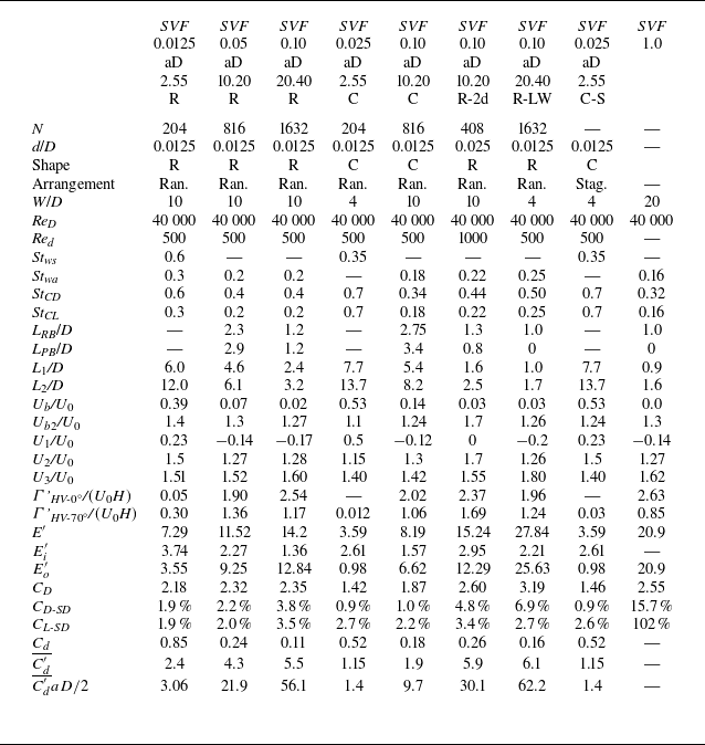

 SVF
 aD
 SVF
 aD
 SVF
 ω¯n
 x/D

 U¯¯
 k¯¯
 U02
 SVF
 d/D
 W/D

 U02
 SVF
 aD
 SVF
 aD
 SVF
 aD
 SVF
 aD

 U02
 SVF
 aD
 SVF
 aD
 SVF
 aD
 SVF


 SVF
 aD
 SVF
 aD
 SVF
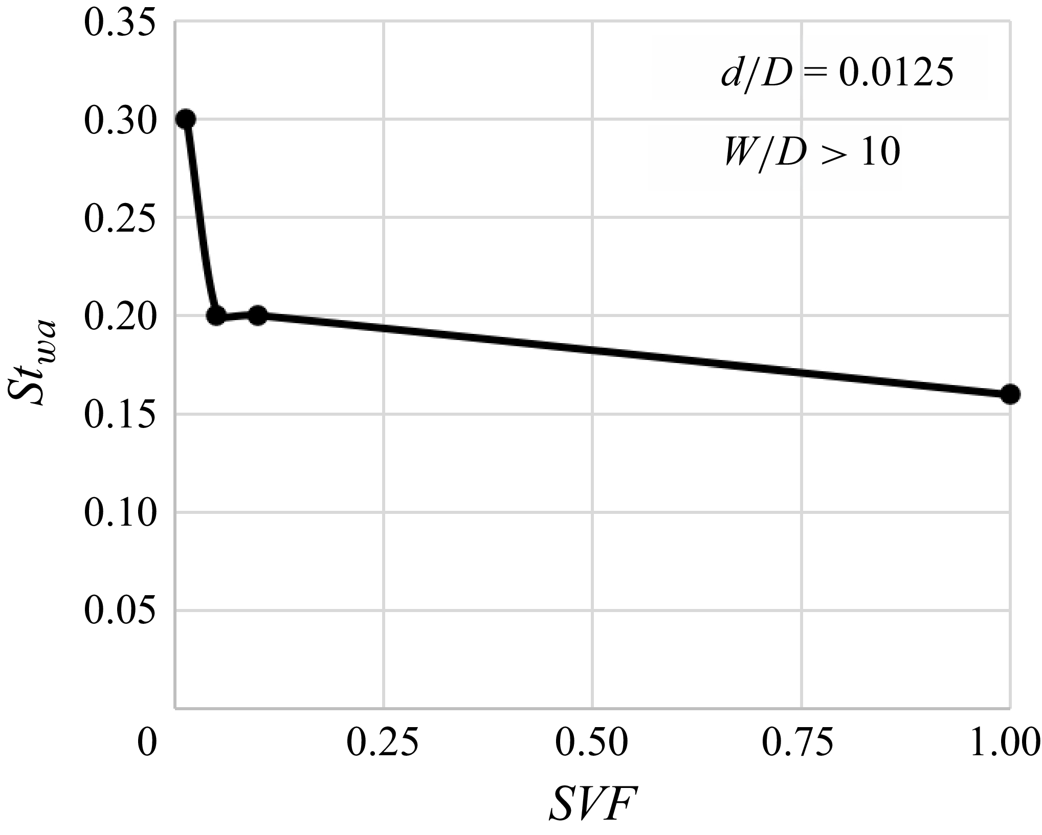
 SVF
 wa

 SVF
 aD

 SVF
 aD
 SVF
 aD

 SVF
 aD
 SVF
 aD

 SVF
 aD
 ω¯x
 SVF
 aD
 ω¯x
 SVF
 aD


 SVF
 d/D
 W/D

 SVF
 aD
 SVF
 aD

 SVF
 aD
 SVF
 aD
 SVF
 aD
 SVF
 aD
 SVF

 τ¯
 τrms
 SVF
 aD
 SVF
 aD
 SVF
 aD
 SVF
 aD
 SVF
 aD
 SVF
 aD
 SVF
 aD
 SVF

 Ei′
 Eo′
 SVF
 d/D
 W/D

 Fx
 ∑Fxbin,i
 Cd′
 ∑Fxbin,i
 U¯¯
 SVF
 d/D
 W/D

 Cd′
 Red¯=U¯¯d/
 SVF
 SVF
 SVF
 Cd′
 Cd′(Red¯
 SVF
 SVF

 Cd′¯
 SVF

 Open access

