1. Introduction
Fluid mixing in turbulence is often conceptualised as a cascade process, where kinetic energy is transferred from large to small scales (Kolmogorov Reference Kolmogorov1991; Frisch Reference Frisch1995; Sreenivasan Reference Sreenivasan2019). The structure function (SF) of scalar fluctuation along the streamwise direction
 $\phi ^\prime$
,
 $S_p(\Delta z) = \langle [\phi ^\prime (z+\Delta z)-\phi ^\prime (z) ]^p \rangle = \langle \Delta \phi ^{\prime p}_{\Delta z}\rangle$
, is frequently studied. Here,
 $\Delta \phi ^{\prime }_{\Delta z}$
is the scalar increment over a separated distance
 $\Delta z$
along the flow direction,
 $p$
is the moment order and
 $\langle \boldsymbol{\cdot }\rangle$
denotes the ensemble average operation. At a large Taylor-microscale Péclet number,
 $\textit{Pe}_{\! \lambda} = \textit{Re}_\lambda \textit{Sc} = u_{\textit{rms}} \lambda _u/\alpha$
(where
 $\textit{Re}_\lambda = u_{\textit{rms}} \lambda _u/\nu$
is the Taylor-microscale Reynolds number, with
 $u_{\textit{rms}}$
the root-mean-square (r.m.s.) of the velocity,
 $\lambda _u$
the Taylor microscale of velocity fluctuation and
 $\nu$
the kinematic viscosity;
 $\textit{Sc}$
is the Schmidt number; and
 $\alpha$
is the mass diffusivity), for length scales far away from both the large forcing scale and the small viscous/diffusive scales, the scalar structure function exhibits scaling behaviour (Obukhov Reference Obukhov1949; Corrsin Reference Corrsin1951),
 \begin{equation} S_p(\Delta z) \sim (\Delta z)^{\xi _p}, \end{equation}
where
 $\xi _p$
is the scaling exponent and is expected to be
 $p/3$
for ideal Kolmogorov-type turbulence. However, the presence of steep scalar gradients, often referred to as cliffs or fronts, leads to spatial intermittency, causing deviations from this scaling and giving rise to anomalous scaling exponents (Frisch Reference Frisch1995; Celani et al. Reference Celani, Lanotte, Mazzino and Vergassola2000; Iyer et al. Reference Iyer, Schumacher, Sreenivasan and Yeung2018). The intermittency of passive scalars has been extensively studied over the past decades through theoretical (e.g. Kraichnan Reference Kraichnan1994; She & Leveque Reference She and Leveque1994; Cao & Chen Reference Cao and Chen1997), numerical (e.g. Cao, Chen & Sreenivasan Reference Cao, Chen and Sreenivasan1996; Watanabe & Gotoh Reference Watanabe and Gotoh2006; Gotoh & Watanabe Reference Gotoh and Watanabe2015; Iyer et al. Reference Iyer, Schumacher, Sreenivasan and Yeung2018; Buaria et al. Reference Buaria, Clay, Sreenivasan and Yeung2021a
) and experimental approaches. Experimental studies have primarily focused on temperature fields with Prandtl numbers (
 $\textit{Pr}$
) (the Prandtl number (the ratio of kinematic viscosity to thermal diffusivity) is analogous to the Schmidt number (
 $\textit{Sc}$
) and they are not distinguished in this study) of order unity, such as in grid turbulence (Gylfason & Warhaft Reference Gylfason and Warhaft2004), heated jet (Antonia et al. Reference Antonia, Hopfinger, Gagne and Anselmet1984), heated wake (Meneveau et al. Reference Meneveau, Sreenivasan, Kailasnath and Fan1990; Lepore & Mydlarski Reference Lepore and Mydlarski2009) and turbulent Rayleigh–Bénard convection (Sun, Zhou & Xia Reference Sun, Zhou and Xia2006; Lohse & Xia Reference Lohse and Xia2010; He, Shang & Tong Reference He, Shang and Tong2014). These studies consistently show nonlinear deviations of
 $\xi _p$
from
 $p/3$
, establishing intermittency as a hallmark of scalar turbulence.
Kraichnan (Reference Kraichnan1994) posed an important question – whether
 $\xi _p$
saturates to a constant at high orders
 $p$
. Phenomenological arguments of the multifractal type suggest a saturation to the asymptotic value
 $\xi _\infty$
(Frisch Reference Frisch1995; Falkovich, Gawȩdzki & Vergassola Reference Falkovich, Gawȩdzki and Vergassola2001). Numerical evidence for such saturation was provided by Celani et al. (Reference Celani, Lanotte, Mazzino and Vergassola2000), who reported
 $\xi _\infty = 1.4$
in simulations of a passive scalar advected by a two-dimensional non-intermittent Navier–Stokes flow subjected to a mean scalar gradient and random forcing. Experimental support followed from Moisy et al. (Reference Moisy, Willaime, Andersen and Tabeling2001), who observed
 $\xi _\infty = 1.45 \pm 0.1$
at
 $p = 10$
in laboratory measurements of passive temperature fluctuations in homogeneous isotropic turbulence (HIT). A three-dimensional direct numerical simulation (DNS) study by Watanabe & Gotoh (Reference Watanabe and Gotoh2006) yielded
 $\xi _\infty = 1.3$
for passive scalar mixing in HIT under a constant mean scalar gradient at
 $\textit{Pe}_{\! \lambda} = 468$
. More recently, using the same configuration, Iyer et al. (Reference Iyer, Schumacher, Sreenivasan and Yeung2018) found
 $\xi _\infty = 1.2$
at
 $\textit{Pe}_{\! \lambda} = 650$
and Buaria et al. (Reference Buaria, Clay, Sreenivasan and Yeung2021a
) extended this to higher
 $\textit{Pe}_{\! \lambda} = 3120$
and reported
 $\xi _\infty \approx 1.1$
. They also demonstrated that
 $\xi _\infty$
decreases with increasing
 $\textit{Pe}_{\! \lambda}$
, proposing that the asymptotic limit approaches
 $\xi _\infty = 1$
as
 $\textit{Pe}_{\! \lambda} \to \infty$
.
Investigations of saturation have predominantly focused on HIT, with DNS limited to a
 $\textit{Pe}_{\! \lambda}$
of
 $\mathcal{O}(10^3)$
. This leaves gaps in experimental validation at higher
 $\textit{Pe}_{\! \lambda}$
and in sheared flows, such as atmospheric boundary layers, channel flows and engineering pipes. While realistic turbulent flows often involve inhomogeneity and anisotropy, which may alter velocity and scalar statistics (Lohse & Xia Reference Lohse and Xia2010), previous studies suggest that, sufficiently far from boundaries and strong shear, intermittency and anomalous scaling can approach HIT-like behaviour (Toschi et al. Reference Toschi, Amati, Succi, Benzi and Piva1999; Benzi et al. Reference Benzi, Amati, Casciola, Toschi and Piva1999). Toschi et al. (Reference Toschi, Amati, Succi, Benzi and Piva1999) used the extended self-similarity (ESS) methodology in channel flow and found that intermittency near the centre (the wall unit coordinate larger than
 $100$
at a bulk Reynolds number
 $\textit{Re} = 3000$
) aligns with that in HIT. For the passive scalar, Celani et al. (Reference Celani, Lanotte, Mazzino and Vergassola2000, Reference Celani, Lanotte, Mazzino and Vergassola2001) showed that large-scale anisotropy persists into dissipative ranges without isotropy fully recovered, yet scalar scaling exponents remain universal, with strong intermittency and saturation at high orders.
Despite these insights, experimental investigations of saturation at high
 $\textit{Pe}_{\! \lambda}$
remain limited, hindering understanding of the asymptotic behaviour of
 $\xi _\infty$
. In this study, the anomalous scaling of passive scalar mixing is examined in turbulent pipe flow experiments at
 $\textit{Pe}_{\! \lambda} \sim \mathcal{O}(10^5)$
, treating approximate streamwise homogeneity and isotropy in the measurement region far from the pipe wall. The experiments are introduced in § 2; the results and discussions are reported in § 3; and the study is summarised in § 4.
2. Experimental method
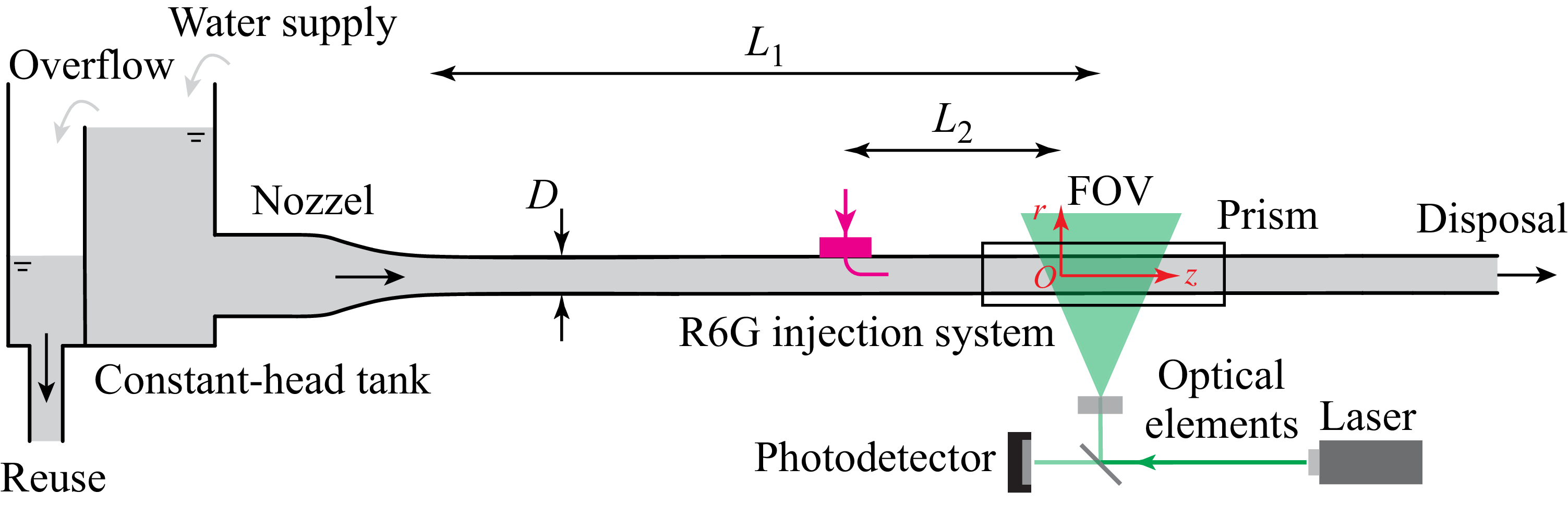
The experimental set-up is sketched in figure 1. A constant-head tank supplied the working fluid to the pipe via a nozzle. The pipe comprises several acrylic segments connected by custom-fabricated connectors. The pipe has an inner diameter of
 $D = 40$
mm and a length of
 $4$
m, corresponding to
 $100D$
. A flow meter and a valve were installed at the pipe outlet. Purified water was used as the working fluid. The flow was driven by gravity with the flow rate controlled by adjusting the outlet valve. The flow was characterised by the bulk Reynolds number,
 $\textit{Re} = U_0D/\nu$
, where
 $U_0$
is the mean flow velocity and
 $\nu$
is the fluid kinematic viscosity. In this study, the bulk Reynolds numbers are
 $\textit{Re} = 10\,000$
,
 $15\,000$
and
 $20\,000$
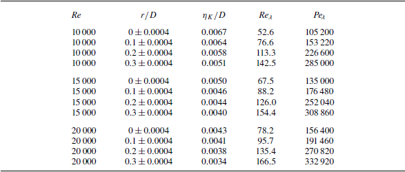
. The velocity field was measured by a two-dimensional particle image velocimetry to estimate the Kolmogorov scales and Taylor microscales in the pipe flow, see Appendix for details. The characteristic flow parameters are summarised in table 1.
Summary of the flow characteristic parameters:
 $\textit{Re}$
is bulk Reynolds number;
 $r/D$
is the radial position;
 $\textit{Re}_\lambda = u_{\textit{rms}} \lambda _u/\nu$
is the Taylor-microscale Reynolds number, where
 $u_{\textit{rms}}$
is the root-mean-square of the velocity,
 $\lambda _u$
the Taylor microscale of velocity fluctuation and
 $\nu$
the kinetic viscosity;
 $\eta _K$
is the Kolmogorov scale;
 $\textit{Pe}_{\! \lambda} =\textit{Re}_\lambda \textit{Sc}$
is the Taylor-microscale Péclet number.

Sketch of the general pipe set-up, where inner diameter
 $D = 40$
mm. The fluid in the pipe is driven by gravity and scalar is discharged by injection through small needle with a 2 mm inner diameter (
 $d$
) at downstream positions
 $L_1-L_2 = 25D$
. The scalar concentration field was measured by PLIF at
 $L_2 = 220d$
downstream from the needle.

A dilute solution of fluorescent dye (Rhodamine 6G, concentration
 $\phi _0 = 100\,{\unicode{x03BC}} \mathrm{g}\,\mathrm{L}^{-1}$
) serves as the passive scalar, with a Schmidt number
 $\textit{Sc}\approx 2000$
(Vanderwel & Tavoularis Reference Vanderwel and Tavoularis2014). The dye is introduced into the turbulent pipe flow via an L-shaped injector, as illustrated schematically in figure 1. The horizontal section of the injector is aligned with the pipe axis at the pipe centre. The injector has an inner diameter of
 $d=2$
mm and an outer diameter
 $2.4$
mm. A gear pump (LEADFLUID
 $^{\circledR}$
, CT3001F) discharges the dye at a precisely controlled flow rate matching the bulk flow velocity, minimising injection disturbances to the turbulent flow. The cylindrical coordinate system is defined so that the origin is located at the intersection of the pipe axis and the left boundary of the measurement field of view. The
 $z$
-axis aligns with the pipe axis, while the
 $r$
-axis is along the radial direction.
To investigate passive scalar mixing in the
 $z$
–
 $r$
plane, the planar laser-induced fluorescence (PLIF) technique is employed to measure the scalar concentration. The measurement field of view covers an area of approximately
 $1.2D \times 1.2D$
, centred around 25
 $D$
(
 $220d$
) downstream from the L-type injector exit. The disturbances caused by the injector and the dye discharge were expected to be negligible. A high-repetition-rate pulsed laser (Beamtech Vlite-Hi-527, operating at
 $1$
kHz) is used for illumination. A laser sheet with an average thickness of
 $200\,{\unicode{x03BC}} \mathrm{m}$
is generated using a series of optical lenses. A beamsplitter is used to separate a portion laser energy to a photodetector (Thorlabs, PDA100A2), which monitors the laser pulse intensity at the same time for posteriorly correcting the measurements caused by the laser intensity fluctuations. Images were recorded by a high-speed camera (PCO, in full resolution of
 $2016\times 2016$
pixels
 $^2$
) at a sampling rate of
 $1\,\mathrm{kHz}$
, while photodetector data were captured at
 $40\,\mathrm{kHz}$
. The averaged photodetector signal for each pulse is used for intensity correction. The configuration of the camera and the laser sheet enables the PLIF measurements to resolve mixing structures larger than the Kolmogorov scale, sufficient for the structure function statistics in this study. For each Reynolds number, approximately
 $10\,000$
PLIF images were acquired, corresponding to a flow duration of approximately
 $60D/U_0$
. The PLIF calibration follows the procedure described by Xu & Chen (Reference Xu and Chen2012). The mean and r.m.s. profiles of the scalar concentration at several streamwise positions are examined. These profiles are nearly identical and independent of streamwise location, and exhibit approximately Gaussian shapes (see Li, Xu & He Reference Li, Xu and He2025), which are consistent with previous experimental results in turbulent channel flows (e.g. Lavertu & Mydlarski Reference Lavertu and Mydlarski2005). More details about the experimental set-up and measurements can be found from Li et al. (Reference Li, Xu and He2025).
3. Results and discussion
3.1. Isotropy assessment
In turbulent pipe flow, where mean shear introduces anisotropy at large scales, verifying isotropy at small scales is essential to ensure that the observed scaling behaviours are not confounded by directional biases. Here, the isotropy of both the velocity and scalar fields is examined using spectral and statistical measures, focusing on radial positions
 $r/D \leqslant 0.3$
, where the flow is expected to approach isotropy from the literature (Toschi et al. Reference Toschi, Amati, Succi, Benzi and Piva1999).
For the velocity field, isotropy is assessed via the spectral coherency
 $H_{zr}(k_z) = |E_{zr}(k_z)|^2 / [E_{zz}(k_z) E_{rr}(k_z)]$
(Saddoughi & Veeravalli Reference Saddoughi and Veeravalli1994), where
 $E_{zz}(k_z)$
and
 $E_{rr}(k_z)$
are the one-dimensional energy spectra of the axial and radial velocity components, respectively, and
 $E_{zr}(k_z)$
is their cross-spectrum. Here,
 $k_z$
is the wavenumber along the axial direction. A value of
 $H_{zr}(k_z) \ll 1$
indicates weak correlation between the components, signifying local isotropy. Figure 2(a) presents the normalised spectra
 $|E_{zr}(k_z)| / (U_0^2 D)$
,
 $E_{zz}(k_z) / (U_0^2 D)$
and
 $E_{rr}(k_z) / (U_0^2 D)$
as functions of
 $k_z \eta _K$
for
 $\textit{Re} = 10\,000$
at
 $r/D = 0$
(centreline) and
 $r/D = 0.3$
. Across the entire wavenumber range,
 $|E_{zr}(k_z)|$
remains approximately an order of magnitude smaller than
 $E_{zz}(k_z)$
and
 $E_{rr}(k_z)$
, suggesting minimal cross-coupling. This qualitative observation is quantified in figure 2(b), which shows
 $H_{zr}(k_z)$
versus
 $k_z \eta _K$
for
 $\textit{Re} = 10\,000$
and
 $20\,000$
at both positions. Notably,
 $H_{zr}(k_z) \ll 1$
for
 $10^{-2} \lt k_z \eta _K \lt 10$
, and even lower in the inertial range, confirming near-isotropy for
 $r \leqslant 0.3D$
. This finding aligns with previous studies in pipe turbulence, such as Cerbus et al. (Reference Cerbus, Liu, Gioia and Chakraborty2020), who reported isotropy for
 $r \leqslant 0.45D$
based on similar spectral analyses. A slight increase in
 $H_{zr}$
at larger
 $r/D$
hints at emerging shear effects, but remains very small to support the isotropy assumptions in our scaling analysis.
(a) Plots of
 $|E_{zr}(k_z)|/(U_0^2D)$
versus
 $k_z \eta _K$
(dotted lines),
 $|E_{zz}(k_z)|/(U_0^2D)$
versus
 $k_z \eta _K$
(solid lines) and
 $|E_{rr}(k_z)|/(U_0^2D)$
versus
 $k_z \eta _K$
(dashed lines) for
 $\textit{Re} = 10\,000$
at
 $r/D = 0$
(top) and
 $r/D = 0.3$
(bottom). (b) Plots of
 $H_{zr}(k_z)$
versus
 $k_z \eta _K$
for
 $\textit{Re} = 10\,000$
and 20 000 at
 $r/D = 0$
(solid lines) and
 $r/D = 0.3$
(dashed lines). Note that
 $H_{zr}(k_z) \ll 1$
for all
 $k_z$
.

Turning to the scalar field, local isotropy is probed through the probability density functions (p.d.f.s) of the normalised scalar gradients
 $\partial _z \phi ' / \langle (\partial _z \phi ')^2 \rangle ^{1/2}$
and
 $\partial _r \phi ' / \langle (\partial _r \phi ')^2 \rangle ^{1/2}$
, as well as the ratio of their r.m.s. (
 $\langle (\partial _r \phi ')^2 \rangle ^{1/2} / \langle (\partial _z \phi ')^2 \rangle ^{1/2}$
). Asymmetry in the p.d.f. of scalar gradients is a sensitive indicator of anisotropy in small-scale mixing, arising from persistent large-scale ramps or mean gradients that violate isotropy (Sreenivasan Reference Sreenivasan1991b
). Numerical simulations have shown that such asymmetries diminish with increasing Schmidt number
 $\textit{Sc}$
, approaching symmetry and thus isotropy at high
 $\textit{Sc}$
(Yeung, Xu & Sreenivasan Reference Yeung, Xu and Sreenivasan2002; Schumacher & Sreenivasan Reference Schumacher and Sreenivasan2003; Buaria et al. Reference Buaria, Clay, Sreenivasan and Yeung2021b
). The gradients are obtained via finite differences from high-resolution measurements. Figure 3(a) displays the p.d.f.s for
 $\textit{Sc} \approx 2000$
and
 $\textit{Re} = 20\,000$
at
 $r/D = 0$
(filled symbols) and
 $0.3$
(hollow symbols) for both streamwise (
 $\partial _z \phi '$
, solid lines) and radial (
 $\partial _r \phi '$
, dashed lines) components. The p.d.f.s exhibit symmetry about zero, quantified in the inset by the asymmetry measure
 $\gamma = |\mathrm{p.d.f.}(\beta ) - \mathrm{p.d.f.}(-\beta )| / [\mathrm{p.d.f.}(\beta ) + \mathrm{p.d.f.}(-\beta )]$
, where
 $\beta$
is the normalised gradient. Values of
 $\gamma \approx 0$
across the range confirm the observed symmetry, consistent with isotropic mixing at high
 $\textit{Sc}$
(Yeung et al. Reference Yeung, Xu and Sreenivasan2002; Schumacher & Sreenivasan Reference Schumacher and Sreenivasan2003; Buaria et al. Reference Buaria, Clay, Sreenivasan and Yeung2021b
). Similar symmetry holds for other
 $\textit{Sc}$
and
 $\textit{Re}$
conditions examined, underscoring the robustness of this feature. Complementing the p.d.f. analysis, figure 3(b) plots
 $\langle (\partial _r \phi ')^2 \rangle ^{1/2} / \langle (\partial _z \phi ')^2 \rangle ^{1/2}$
versus
 $r/D$
for
 $\textit{Re} = 10\,000$
,
 $15\,000$
and
 $20\,000$
. The ratio remains close to unity (within 1.1) for all cases, deviating only slightly at
 $r/D = 0.3$
– likely due to intensified shear near the wall. This near-unity value supports local isotropy, implied from the circumstance of velocity fluctuations (e.g. Comte-Bellot & Corrsin Reference Comte-Bellot and Corrsin1966; Cerbus et al. Reference Cerbus, Liu, Gioia and Chakraborty2020).
(a) Probability density functions of the normalised streamwsie scalar derivative (
 $\partial _z \phi ^\prime$
) and the normalised radial scalar derivative (
 $\partial _r \phi ^\prime$
, dashed lines) for
 $\textit{Sc} \approx 2000$
and
 $\textit{Re} = 20\,000$
at
 $r/D = 0.0$
(filled symbols) and 0.3 (hollow symbols). The inset shows the quantity
 $ \gamma = |\mathrm{p.d.f.}(\beta )-\mathrm{p.d.f.}(-\beta )|/[\mathrm{p.d.f.}(\beta )+\mathrm{p.d.f.}(-\beta )]$
, where
 $\beta = \partial _z \phi ^\prime /\langle (\partial _z \phi ^\prime )^2\rangle ^{1/2}$
or
 $\partial _r \phi ^\prime /\langle (\partial _r \phi ^\prime )^2\rangle ^{1/2}$
. Smaller values of this quantity indicate smaller asymmetries. (b) The ratio,
 $\langle (\partial _r \phi ^\prime )^2 \rangle ^{1/2}/ \langle (\partial _z \phi ^\prime )^2 \rangle ^{1/2}$
, versus
 $r/D$
for
 $\textit{Re} = 10\,000, 15\,000$
and 20 000.

Overall, these checks affirm that both velocity and scalar fields are approximately locally isotropic in the inertial range for
 $r/D \leqslant 0.3$
. This isotropy is crucial for comparing our results with those from homogeneous isotropic turbulence simulations, bridging experimental and numerical insights into scalar intermittency.
3.2. Structure function
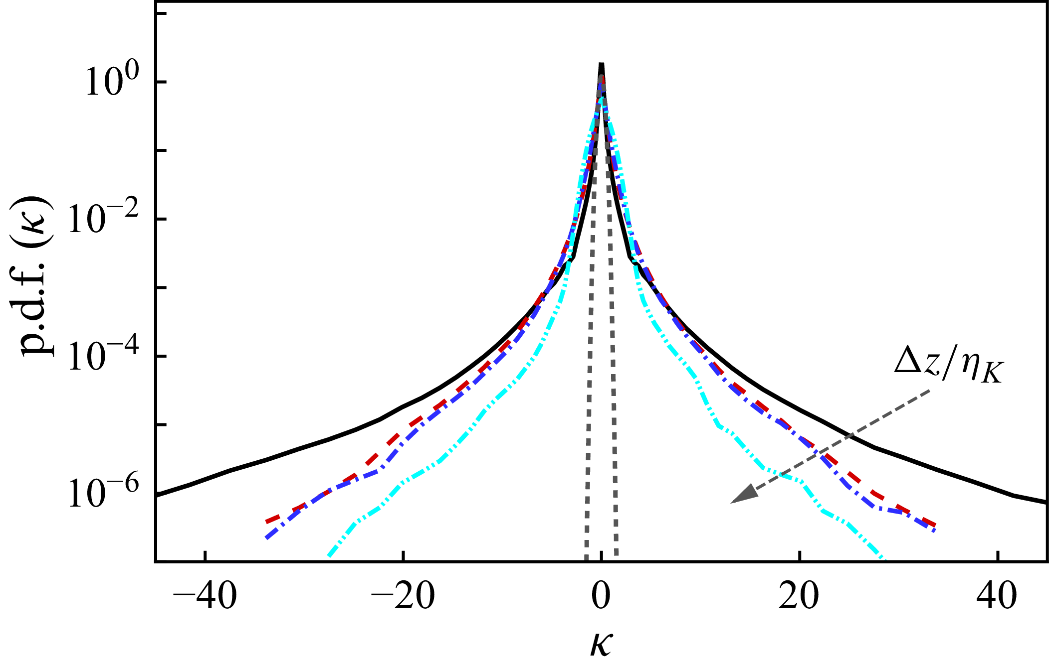
The small-scale intermittency of scalar fluctuations is characterised by the p.d.f. of scalar increments at different length scales. Figure 4 presents the p.d.f.s of
 $\kappa =S_1/\sigma _1$
for separations
 $\Delta z$
, ranging from
 $\Delta z/\eta _K = 1$
to
 $200$
, where
 $\eta _K$
is the Kolmogorov scale and
 $\sigma _1$
the corresponding standard deviation of the first-order structure function
 $S_1$
. These p.d.f.s show significant deviations from Gaussian distributions, with pronounced non-Gaussian tails indicative of strong intermittency. Additionally, the distributions exhibit approximate symmetry, which is consistent with the finding of recovery of local isotropy at high Schmidt numbers (e.g. Yeung et al. Reference Yeung, Xu and Sreenivasan2002; Brethouwer, Hunt & Nieuwstadt Reference Brethouwer, Hunt and Nieuwstadt2003; Schumacher & Sreenivasan Reference Schumacher and Sreenivasan2003; Buaria et al. Reference Buaria, Clay, Sreenivasan and Yeung2021a
). This behaviour differs from the findings in low-Schmidt-number (
 $\textit{Sc} \sim 1$
) studies (e.g. Warhaft Reference Warhaft2000; Moisy et al. Reference Moisy, Willaime, Andersen and Tabeling2001), where small-scale anisotropy persists.
Probability density functions of the normalised scalar increments
 $\kappa = S_1/\sigma _1$
at
 $\textit{Pe}_{\! \lambda} =156\,400$
, where
 $\sigma _1$
is the standard deviation of
 $S_1$
. From the outer to the inner p.d.f.,
 $\Delta z/\eta _K = 1, 10, 100$
and
 $200$
. The grey dashed line indicates a Gaussian distribution.

Figure 5(a) presents the scalar structure functions along the streamwise direction,
 $S_p(\Delta z) = \langle \Delta \phi ^{\prime p}_{\Delta z}\rangle$
, measured at
 $\textit{Pe}_{\! \lambda} =156\,400$
. Within the range
 $10 \lesssim \Delta z/\eta _K \lesssim 100$
, the structure functions exhibit power-law scaling,
 $S_p(\Delta z) \sim (\Delta z)^{\xi _p}$
. Figure 5(b) shows the corresponding local slope of the structure functions,
 $G_p = \mathrm{d}[\mathrm{log}(S_p/\phi '^p_{\textit{rms}})]/{} \mathrm{d}[\mathrm{log}(\Delta z/\eta _K)]$
, where
 $\phi '_{\textit{rms}}$
is the root-mean-square of the scalar fluctuation. The corresponding slope remains approximately constant in the selected scale range (marked by the grey area), suggesting reasonably defined power-law behaviour. To further verify homogeneity, the measurement domain was divided into upstream and downstream halves, and the structure functions were computed for each section independently. The resulting structure functions from both halves are nearly identical (data not shown), demonstrating that the scalar statistics are statistically homogeneous in the streamwise direction. The extended self-similarity (ESS) methodology introduced by Benzi et al. (Reference Benzi, Ciliberto, Tripiccione, Baudet, Massaioli and Succi1993) leverages the hierarchical relationships among the structure functions to extend the effective scaling range, particularly beneficial in flows where the inertial range might be constrained with insufficiently large
 $\textit{Re}_\lambda$
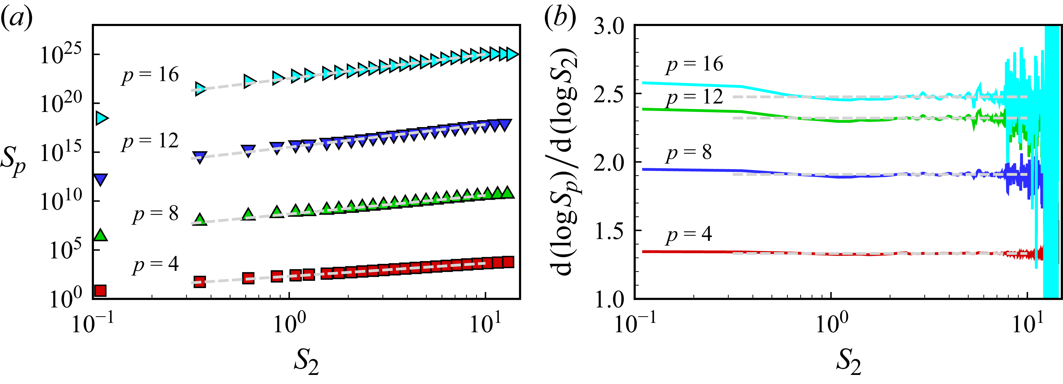
(e.g. Benzi et al. Reference Benzi, Ciliberto, Tripiccione, Baudet, Massaioli and Succi1993; Ruiz-Chavarria, Baudet & Ciliberto Reference Ruiz-Chavarria, Baudet and Ciliberto1996; Toschi et al. Reference Toschi, Amati, Succi, Benzi and Piva1999; Arad et al. Reference Arad, Biferale, Mazzitelli and Procaccia1999). Figure 6(a) shows the structure functions
 $S_p$
(
 $p = 4, 8, 12, 16$
) plotted against
 $S_2$
. The near-linear arrangement observed in the log–log plot of figure 6(a) provides a compelling visual confirmation of this extended scaling. Additionally, figure 6(b) illustrates the corresponding local slopes,
 $\mathrm{d} [\log S_p] / \mathrm{d} [\log S_2] = \mathrm{d} \xi _p / \mathrm{d} \xi _2$
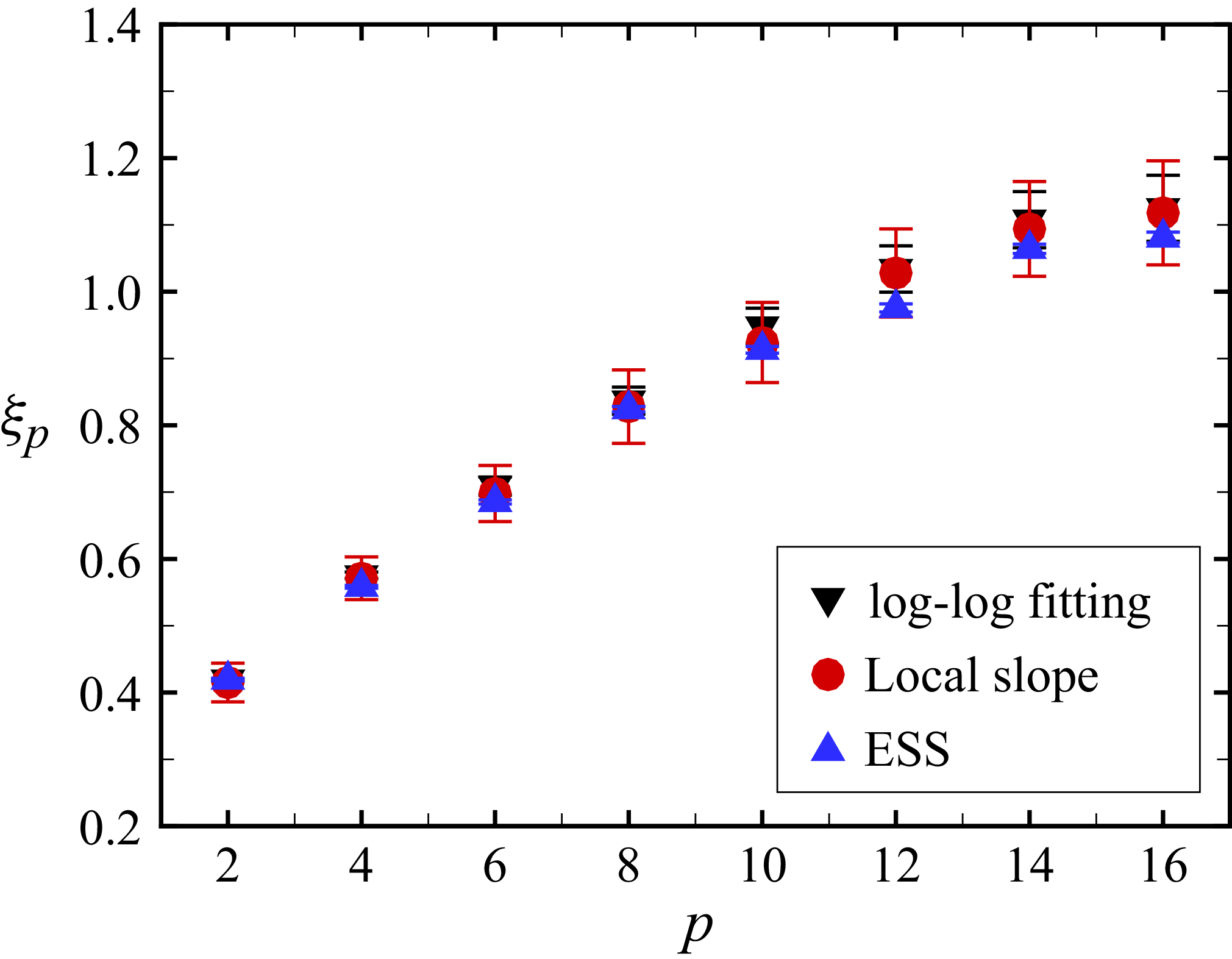
, which exhibit a nearly constant profile across the designated range. This stability in the local slope reinforces the robustness and reliability of the structure function scaling (Ruiz-Chavarria et al. Reference Ruiz-Chavarria, Baudet and Ciliberto1996; Warhaft Reference Warhaft2000). The exponents of the structure functions obtained using the log–log fitting, the mean of the local slope and the ESS are summarised in figure 7. The exponents from the three methods are very close, typically varying by less than 4 % indicating that the influence of the method choice on the results is trivial.
(a) Normalised scalar structure functions along streamwise direction (from
 $p = 2$
to 16) at
 $\textit{Pe}_{\! \lambda} =156\,400$
. (b) Corresponding local slope of
 $p$
th-order scalar structure functions. The grey region indicates the scale range for calculating the scaling exponents.

(a) Scalar structure functions
 $S_p$
(
 $p = 4, 8, 12, 16$
, from bottom to top) versus
 $S_2$
at
 $\textit{Pe}_{\! \lambda} =156\,400$
. The grey dashed lines indicate the selected extended self-similarity (ESS) range. (b) Corresponding local slope of
 $p$
th-order structure functions in ESS.

Scaling exponents of the structure functions estimated by the log–log fitting (figure 5
a), the mean of the local slope (figure 5
b) and ESS (figure 6
a) at
 $\textit{Pe}_{\! \lambda} = 156\,400$
. The respective
 $95\,\%$
confidence intervals from the log–log fitting and the ESS fitting are taken as error bars. The standard deviation of the local slopes is taken as the error bars.

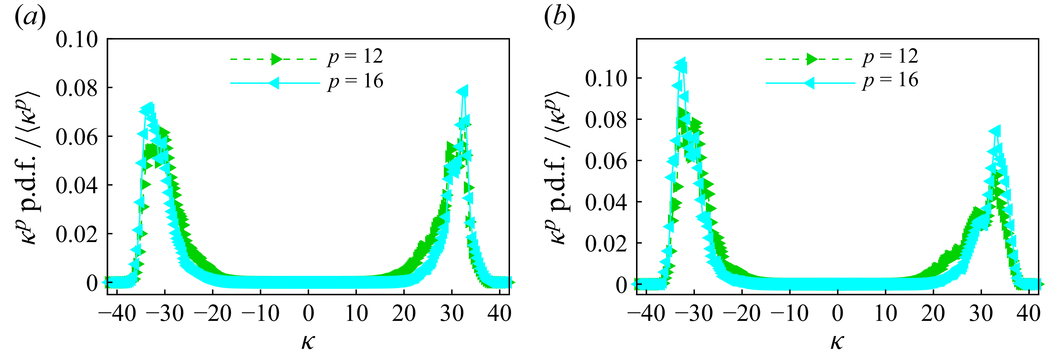
Statistical convergence is examined by the classic moment integrands,
 $\kappa ^p \mathrm{p.d.f.}(\kappa )$
, as shown in figures 8(a) and 8(b) for
 $\Delta z/ \eta _K = 15$
and
 $\Delta z/ \eta _K = 90$
, respectively. Each integrand exhibits a distinct peak (at
 $\kappa \approx 30$
) before decaying in the tail, ensuring the contributions from higher-order moments are statistically convergent (e.g. Celani et al. Reference Celani, Lanotte, Mazzino and Vergassola2000, Reference Celani, Lanotte, Mazzino and Vergassola2001; Iyer et al. Reference Iyer, Schumacher, Sreenivasan and Yeung2018).
Integrands of scalar increment moments as functions of scalar increments at (a)
 $\Delta z/\eta _K = 15$
and (b)
 $\Delta z/\eta _K = 90$
.

Power-law fitting was applied to the structure functions within the selected scale range to obtain scaling exponents
 $\xi _p$
(see figure 5
a), which are shown as a function of the moment order
 $p$
for different
 $\textit{Pe}_{\! \lambda}$
in figure 9(a), along with the results of homogeneous isotropic turbulence for comparisons. In figure 9(a), the measured
 $\xi _p$
deviates from the linear prediction
 $p/3$
of Kolmogorov–Obukhov–Corrsin theory (Obukhov Reference Obukhov1949; Corrsin Reference Corrsin1951; Kolmogorov Reference Kolmogorov1991), and potentially contributed to large-scale anisotropy in shear flows, scalar initial conditions and other factors (e.g. Sreenivasan Reference Sreenivasan1991a
; Lohse Reference Lohse1994; Antonia, Zhou & Xu Reference Antonia, Zhou and Xu2000; Lepore & Mydlarski Reference Lepore and Mydlarski2009). As
 $p$
increases,
 $\xi _p$
increases and gradually begins at high moment orders to approach an approximate saturation scaling exponent
 $\xi _\infty$
. (The difference between the highest two orders, i.e.
 $\xi _{16}$
and
 $\xi _{14}$
, is less than approximately
 $2\,\%$
, similar to Moisy et al. (Reference Moisy, Willaime, Andersen and Tabeling2001), Iyer et al. (Reference Iyer, Schumacher, Sreenivasan and Yeung2018) and Buaria et al. (Reference Buaria, Clay, Sreenivasan and Yeung2021a
).) In figure 9(b), the approximate saturation
 $\xi _\infty$
can be seen to decrease as
 $\textit{Pe}_{\! \lambda}$
increases, in agreement with Buaria et al. (Reference Buaria, Clay, Sreenivasan and Yeung2021a
)’s observation in homogeneous isotropic turbulence. The data from different background flow shear, denoted by
 $|\partial \langle U\rangle /\partial r|$
, indicate that
 $\xi _\infty$
does not have a clear dependence on the flow shear, but mainly on
 $\textit{Pe}_{\! \lambda}$
. The inset of figure 9(b) shows that
 $\xi _\infty (\textit{Pe}_{\! \lambda} )$
in the homogeneous isotropic turbulence clearly differs from that in pipe flows, suggesting that other factors may have associations with the saturation scaling exponents. The extent of intermittency may be the possible cause, implied by more flattened tails of p.d.f.(
 $\kappa$
) in this study (see figure 4) than in the literature (e.g. Chen & Kraichnan Reference Chen and Kraichnan1998; Celani et al. Reference Celani, Lanotte, Mazzino and Vergassola2000; Gylfason & Warhaft Reference Gylfason and Warhaft2004; Gotoh & Yeung Reference Gotoh and Yeung2012), and is worthy of a future investigation. Notably, the anomalous scaling can be predicted by zero-mode theory (where the scalar diffusivity tends to zero) within the Kraichnan model for scalar turbulence (Gawȩdzki & Kupiainen Reference Gawȩdzki and Kupiainen1995; Falkovich et al. Reference Falkovich, Gawȩdzki and Vergassola2001). The early two-dimensional simulation of passive scalar mixing shows
 $\xi _\infty =1.4$
in the energy inverse cascade range (without mentioning the Schmidt number) (Celani et al. Reference Celani, Lanotte, Mazzino and Vergassola2000, Reference Celani, Lanotte, Mazzino and Vergassola2001), where the velocity field is close to Gaussian. In three-dimensional simulations, the velocity field is more intermittent and Watanabe & Gotoh (Reference Watanabe and Gotoh2006) evidence
 $\xi _\infty \approx 1.3$
for
 $\textit{Sc}=1$
(
 $\textit{Re}_\lambda =468$
giving
 $\textit{Pe}_{\! \lambda} =468$
). This implies that there is no universal
 $\xi _\infty$
. Recent three-dimensional simulations of Iyer et al. (Reference Iyer, Schumacher, Sreenivasan and Yeung2018) and Buaria et al. (Reference Buaria, Clay, Sreenivasan and Yeung2021b
) show smaller
 $\xi _\infty$
at larger
 $\textit{Pe}_{\! \lambda}$
and importantly demonstrate that the dependence of
 $\xi _\infty$
on
 $\textit{Pe}_{\! \lambda}$
; see inset of figure 9(b). Notably, the data obtained at the pipe centreline (white-filled symbols in figure 9
b), where the flow approximates homogeneous isotropic turbulence (HIT), exhibit a decrease in
 $\xi _\infty$
with increasing
 $\textit{Pe}_{\! \lambda}$
. This trend is consistent with the global dataset, which similarly indicates a reduction in
 $\xi _\infty$
at higher
 $\textit{Pe}_{\! \lambda}$
, notwithstanding the experimental scatter. However, this observation does not imply that inhomogeneity and anisotropy are negligible. As detailed in the review by Biferale & Procaccia (Reference Biferale and Procaccia2005), extracting universal scaling exponents from experiments is difficult due to finite-diffusivity effects and the persistence of anisotropy. In particular, the narrowing gap between isotropic and anisotropic scaling exponents at high orders suggests that anisotropic modes may contaminate high-order statistics. Although the mean scalar profile
 $\langle \phi \rangle$
was subtracted in this study to mitigate large-scale anisotropy (Shraiman & Siggia Reference Shraiman and Siggia1994), residual anisotropic effects likely persist. A definitive assessment of universality requires systematically isolating these contributions, either via cross-structure functions of velocity and scalar fluctuations (He et al. Reference He, Shang and Tong2014) or through a decomposition of statistical quantities (e.g. Arad et al. Reference Arad, Dhruva, Kurien, L’vov, Procaccia and Sreenivasan1998, Reference Arad, Biferale, Mazzitelli and Procaccia1999; Benzi et al. Reference Benzi, Amati, Casciola, Toschi and Piva1999; Toschi, Lévêque & Ruiz-Chavarria Reference Toschi, Lévêque and Ruiz-Chavarria2000).
(a) Scaling exponent
 $\xi _p$
as a function of the moment order
 $p$
for three
 $\textit{Pe}_{\! \lambda}$
from this study and reference studies. Error bars represent the 95 % confidence intervals. The dashed line
 $\xi _p = p/3$
corresponds to the Kolmogorov–Obukhov–Corrsin phenomenology. The dotted line with an arrow indicates the approximate saturation. (b) Saturation scaling exponent
 $\xi _\infty$
colour-coded with the background velocity gradient along the pipe radius as a function of
 $\textit{Pe}_{\! \lambda}$
. The inset shows
 $\xi _\infty (\textit{Pe}_{\! \lambda} )$
of the passive scalar mixing in homogeneous isotropic turbulence (HIT) from Moisy et al. (Reference Moisy, Willaime, Andersen and Tabeling2001), Watanabe & Gotoh (Reference Watanabe and Gotoh2006), Iyer et al. (Reference Iyer, Schumacher, Sreenivasan and Yeung2018) and Buaria et al. (Reference Buaria, Clay, Sreenivasan and Yeung2021a
), as well as the pipe flow in this study.

3.3. Saturation and co-dimension of sharp fronts
The saturation of scaling exponents in structure functions is well recognised as a hallmark of statistics dominated by shocklike structures, i.e. sharp scalar fronts. These fronts, characterised by abrupt changes in scalar concentration, play a crucial role in shaping the intermittent behaviour observed in high-order moments.
An alternative analytical approach involves examining, for a fixed value of the first-order structure function
 $S_1(\Delta z)$
, how the p.d.f. of the normalised scalar differences
 $S_1(\Delta z) / \phi '_{\textit{rms}}$
evolves with varying separation distances
 $\Delta z$
. The concept of saturation in scaling exponents at higher orders suggests that, for scalar increments
 $\Delta \phi '_{\Delta z}$
significantly exceeding the root-mean-square scalar fluctuation
 $\phi '_{\textit{rms}}$
, the p.d.f. of
 $S_1(\Delta z) / \phi '_{\textit{rms}}$
should adopt a form proportional to
 $(\Delta z / \eta _K)^{-\xi _\infty }$
, where
 $\xi _\infty$
represents the saturation exponent (Celani et al. Reference Celani, Lanotte, Mazzino and Vergassola2000; Iyer et al. Reference Iyer, Schumacher, Sreenivasan and Yeung2018). Figure 10 illustrates that the normalised quantity
 $S_1(\Delta z) / \phi '_{\textit{rms}}$
exhibits a consistent collapse across the scale separations in the inertial-convective range, particularly when
 $S_1(\Delta z) \gtrsim 10 \phi '_{\textit{rms}}$
. This observed collapse serves as additional evidence supporting the saturation of high-order scalar structure function exponents.
Probability density function of scalar increments at
 $r/D = 0$
for Re = 20 000 across the inertial range, multiplied by
 $(\Delta z)^{-\xi _\infty }$
, where
 $-\xi _\infty$
is the saturation exponent (see figure 9
a). The p.d.f. tails collapse, confirming saturation of exponents.

Additionally, Iyer et al. (Reference Iyer, Schumacher, Sreenivasan and Yeung2018) and Buaria et al. (Reference Buaria, Clay, Sreenivasan and Yeung2021a
) demonstrated that the saturation exponent
 $\xi _\infty$
and the box-counting dimension
 $D_{\!F}$
of sharp scalar fronts sum to the Euclidean dimension of the flow, i.e.
 $\xi _\infty + D_{\!F} = 2$
, in the two-dimensional measurement. Following this framework, the box counting method is applied to the sharp scalar fronts to obtain
 $N(\Delta z)$
, the number of squares in dimension of
 $\Delta z$
containing the scalar fronts. The sharp fronts are given by strong scalar gradients
 $\mathscr{R} \equiv \partial _r \phi ^\prime / (\phi ^\prime _{\textit{rms}}/\eta _K )$
, indicated in figure 11(a) and visualised in figure 12, satisfying some chosen thresholds. In figure 11(b),
 $N(\Delta z)$
compensated by the corresponding
 ${(\Delta z)}^{D_{\!F}}$
for each bulk Reynolds number is plotted versus
 $\Delta z$
. Here,
 $D_{\!F}=2{-}\overline {\xi _\infty }$
is used where
 $\overline {\xi _\infty }$
is the average of
 $\xi _\infty$
over
 $0\leqslant r/D \leqslant 0.3$
, representing some sort of overall saturation scaling exponent for each Reynolds number. Notably, at small scales, the curve of
 $\textit{Re}=10\,000$
approaches a plateau, and this gets increasingly more distinct for
 $\textit{Re}=15\,000$
and
 $20\,000$
. This experimentally confirms that the fractal dimension of sharp scalar fronts corresponds to the codimension of the saturation scaling exponent in scalar structure functions. In figure 11(c), the compensated
 $N(\Delta z)$
is plotted for different sharp extents of the front structures. A sharper front structure (as visualised in figure 12, for examples) results in a more distinct plateau that can be observed at small separation scales (see figure 11
c), suggesting that the very sharp front structures give dominant contribution to the saturation scaling exponent.
(a) Probability density function of the normalised scalar gradient,
 $\mathscr{R} \equiv \partial _r \phi ^\prime /(\phi ^\prime _{\textit{rms}}/\eta _K)$
, where dotted lines denote
 $ |\mathscr{R}| = 0.2, 0.4$
and
 $0.6$
, respectively. (b, c) Compensated plot of
 $\langle N\rangle$
, the number of squares in dimension of
 $\Delta z$
containing the scalar fronts satisfying the threshold condition.

Sharp scalar fronts with
 $ |\mathscr{R}| = (a)\, 0.2$
, (b)
 $0.4$
and (c)
 $0.6$
for a snapshot at
 $\textit{Re} = 20\,000$
and
 $\textit{Sc} = 2000$
.

4. Conclusion
The saturation of the scaling exponents, regarding the anomalous scaling of the structure functions of passive scalar, has been evidenced in Taylor-scale Péclet number of
 $\mathcal{O}(10^3)$
homogeneous isotropic turbulence in a limited number of studies and most of them are from numerical simulations. This work presents an experimental study of the passive scalar mixing in turbulent pipe flows, which differ from the homogeneous isotropic turbulence, characterised by its non-trivial velocity gradient along the pipe radius and associated local anisotropy; importantly, this study has Taylor-scale Péclet numbers of
 $\mathcal{O}(10^5)$
. The analysis of structure functions of the passive scalar fluctuation has been carried out along the streamwise direction at the radial positions away from the wall, where the turbulence is close to isotropy. The structure functions of passive scalar fluctuations exhibit anomalous scaling, with the scaling exponent increasing and tending towards saturation as the moment order rises. As the Taylor-scale Péclet number increases, the saturation scaling exponent decreases towards unity, a trend consistent with direct numerical simulations of passive scalar mixing in homogeneous isotropic turbulence. This saturation is further corroborated by the fractal codimension of sharp scalar fronts, which highlights their crucial role in shaping high-order intermittency in the scalar mixing in this flow. Although the mean scalar field
 $\langle \phi \rangle$
was subtracted to mitigate large-scale anisotropy (following Shraiman & Siggia (Reference Shraiman and Siggia1994)), the estimated scaling exponents may still be influenced by sub-leading contributions arising from residual anisotropy, weak inhomogeneity and finite Péclet number effects. Specifically, the measured structure functions likely comprise a superposition of isotropic and anisotropic sectors, as detailed by Arad et al. (Reference Arad, Biferale, Mazzitelli and Procaccia1999) and the comprehensive review by Biferale & Procaccia (Reference Biferale and Procaccia2005). Consequently, further investigations are necessary to systematically isolate these contributions via a decomposition, such as adopting the methodologies established by Arad et al. (Reference Arad, Dhruva, Kurien, L’vov, Procaccia and Sreenivasan1998, Reference Arad, Biferale, Mazzitelli and Procaccia1999), Benzi et al. (Reference Benzi, Amati, Casciola, Toschi and Piva1999) and Toschi et al. (Reference Toschi, Lévêque and Ruiz-Chavarria2000).
Acknowledgements
H.L. would like to acknowledge the experimental support provided by Ms. Haihan Liu. The authors express their gratitude for insightful discussions with Professor H. Xu (Tsinghua University) and Professor J. Xie (Peking University).
Funding
This work was supported by NSFC Excellence Research Group Program for ‘Multiscale Problems in Nonlinear Mechanics’ (No. 12588201) and National Natural Science Foundation of China (Nos. 12372224 and 92152106), Chinese Academy of Sciences (Project for Young Scientists in Basic Research, No. YSBR-087; Strategic Priority Research Program, No. XDB0620102) and China Postdoctoral Science Foundation (Nos. 2023M733589 and 2025T180520).
Declaration of interests
The authors report no conflict of interest.
Data availability statement
The data that support the findings of this study are available upon a reasonable request to the corresponding author.
Author contributions
H.L.: Performed and implemented the experiments, prepared the figures, wrote and reviewed the manuscript. D.X.: Conceptualised the study, guided the experiments, wrote and reviewed the manuscript. G.H.: Discussed, wrote and reviewed the manuscript.
Appendix. Flow velocity characteristics
The velocity fields of the turbulent pipe flows were measured by two-dimensional particle image velocimetry (PIV). The measurement field-of-view is approximately the same as the PLIF measurement, while the same high-speed camera and laser were used. The optical lenses were adjusted to generate the laser sheet of approximately
 $1$
mm thickness. The hollow glass spheres with a medium diameter of approximately
 $11$
 ${\unicode{x03BC}}$
m were used as the tracers. A multi-step correlation algorithm was used to extract the displacement field in Lavision Davis software. The interrogation window size at the final step was set to 32 pixels
 $\times$
32 pixels
 $^2$
with a 50 % overlap. The image sampling rate was adjusted for each flow Reynolds number, so that the maximum displacement is approximately one-quarter of the interrogation window size at the final step (Raffel et al. Reference Raffel, Willert, Scarano, Kähler, Wereley and Kompenhans2018). Approximately 20 000 snapshots of the PIV velocity fields were captured for each Reynolds number.
To estimate
 $\lambda$
for Taylor-scale Reynolds number, the autocorrelation of the streamwise velocity
 $R_{uu}(\Delta z)$
is obtained and a parabola function
 $R_{uu}=1-(\Delta z/\lambda _u)^2$
is applied to the three points of
 $R_{uu}$
close to
 $\Delta z=0$
to extract
 $\lambda _u$
(Pope Reference Pope2000; He, Jin & Yang Reference He, Jin and Yang2017; Mohaghar, Dasi & Webster Reference Mohaghar, Dasi and Webster2020). The dissipation rate
 $\epsilon$
is estimated using the two-dimensional PIV data with assumptions of local axisymmetry (Doron et al. Reference Doron, Bertuccioli, Katz and Osborn2001). The estimated dissipation rate is used to estimate the Kolmogorov length scale
 $\eta _K = (\nu ^3/\epsilon )^{1/4}$
. The estimated Kolmogorov length scales at the pipe centre agree with the data reported by Bailey et al. (Reference Bailey, Hultmark, Schumacher, Yakhot and Smits2009) and Cerbus et al. (Reference Cerbus, Liu, Gioia and Chakraborty2020).