Implications
The model LiGAPS-Beef presented in this paper simulates potential (i.e. the theoretical maximum) and feed-limited production of beef cattle. The difference between the potential or feed-limited production and the actual production is defined as the yield gap. LiGAPS-Beef is designed to quantify yield gaps for different beef production systems across the globe, and identifies the biophysical factors that define cattle growth under potential production and limit growth under feed-limited production. Yield gap analysis, which includes the identification of these factors, can provide insights in the options to increase beef production and resource use efficiency in a sustainable way.
Introduction
Global demand for agricultural products is expected to increase by 60% between 2007 and 2050. In the same period, the estimated increase is even larger for the animal-source foods milk (+62%), eggs (+65%) and meat (+76%), the latter includes +43% for pork, +66% for beef and +123% for poultry meat. At the same time, the projected expansion of global arable land is only 7% (Alexandratos and Bruinsma, Reference Alexandratos and Bruinsma2012). Meeting the future demand for food, therefore, requires an increase in agricultural production per unit of land (Van Ittersum et al., Reference Van Ittersum, Cassman, Grassini, Wolf, Tittonell and Hochman2013), even if food waste is reduced and more plant-based diets are consumed in developed countries.
The future scope to increase agricultural production per unit of land is determined by biophysical, socio-economic, cultural and ethical factors. Biophysical determinants for agricultural activities are relatively conservative since they are governed by biological and physical laws. Improving the biophysical potentials of crops and livestock requires breeding programmes that take multiple years or even decades. Economic or policy constraints are more variable in time and can be managed to some extent. Hence, the biophysical determinants of agricultural production provide a relatively stable benchmark to assess the scope to increase food production towards 2050 under varying economic and policy conditions.
The biophysical scope to increase agricultural production can be assessed by applying concepts of production ecology, which distinguish a hierarchy of production levels. The potential production of crops and livestock is obtained under ideal management, and is determined by genotype and climate only. The next level is referred to as limited production, where water or nutrient availability limits crop growth, and where drinking water, feed quality or available feed quantity limits livestock growth (Van de Ven et al., Reference Van de Ven, de Ridder, van Keulen and van Ittersum2003; Van Ittersum et al., Reference Van Ittersum, Cassman, Grassini, Wolf, Tittonell and Hochman2013; Van der Linden et al., Reference Van der Linden, Oosting, Van de Ven, De Boer and Van Ittersum2015). The actual production is the production level of crops and livestock realised by farmers. In addition to the limiting factors, actual crop production can be reduced by pests, diseases and weeds, whereas actual livestock production can be reduced by diseases and stress (Van Ittersum and Rabbinge, Reference Van Ittersum and Rabbinge1997; Van de Ven et al., Reference Van de Ven, de Ridder, van Keulen and van Ittersum2003; Van der Linden et al., Reference Van der Linden, Oosting, Van de Ven, De Boer and Van Ittersum2015). The difference between the potential or limited production and the actual production is defined as the yield gap. Quantification of yield gaps thus indicates how much agricultural production can be increased from a biophysical perspective (Lobell et al., Reference Lobell, Cassman and Field2009, Van Ittersum et al., Reference Van Ittersum, Cassman, Grassini, Wolf, Tittonell and Hochman2013).
Mechanistic models simulating crop growth provide a suitable means to estimate potential and limited crop production under different conditions (Lobell et al., Reference Lobell, Cassman and Field2009), and, therefore, are the backbone of yield gap analysis. Such models simulate interactions among crop genotype, climate, water and nutrients, and identify the biophysical factors contributing most to yield gaps (Bouman et al., Reference Bouman, van Keulen, van Laar and Rabbinge1996). The yield gap can be attributed to each of the factors: water limitation, nutrient limitation and the influence of pests, diseases and weeds. Given the relative importance of the factors that define and limit growth, strategies to mitigate yield gaps and increase resource use efficiency can be evaluated (Van Ittersum and Rabbinge, Reference Van Ittersum and Rabbinge1997). Identifying regions with a large scope for production increase is crucial to increase future food production (Van Ittersum et al., Reference Van Ittersum, Cassman, Grassini, Wolf, Tittonell and Hochman2013).
Mechanistic models simulating livestock growth and production based on animal genotype, climate, feed quality or available feed quantity are widely available for different livestock species and types (Freer et al., Reference Freer, Moore and Donnelly1997; Johnson et al., Reference Johnson, Chapman, Snow, Eckard, Parsons, Lambert and Cullen2008; Van Milgen et al., Reference Van Milgen, Valancogne, Dubois, Dourmad, Seve and Noblet2008; Rufino et al., Reference Rufino, Herrero, Van Wijk, Hemerik, De Ridder and Giller2009). Few models refer explicitly to the (genetic) potential production of livestock and/or feed-limited production (Wellock et al., Reference Wellock, Emmans and Kyriazakis2004; Rufino et al., Reference Rufino, Herrero, Van Wijk, Hemerik, De Ridder and Giller2009). Examples of yield gap analyses using such models include those at the farm level for smallholder dairy farms in Mexico with the model FarmDESIGN (Cortez-Arriola et al., Reference Cortez-Arriola, Groot, Massiotti, Scholberg, Aguayo, Tittonell and Rossing2014), and at the household level for smallholder dairy farms in Ethiopia and India with the integrated analysis tool (Mayberry et al., Reference Mayberry, Ash, Prestwidge, Godde, Henderson, Duncan, Blummel, Reddy and Herrero2017). However, to our knowledge, concepts of production ecology (Van de Ven et al., Reference Van de Ven, de Ridder, van Keulen and van Ittersum2003; Van der Linden et al., Reference Van der Linden, Oosting, Van de Ven, De Boer and Van Ittersum2015) are only included explicitly in the model LIVSIM (LIVestock SIMulator), a model simulating dairy production in smallholder farming systems in sub-Saharan Africa (Rufino et al., Reference Rufino, Herrero, Van Wijk, Hemerik, De Ridder and Giller2009). LIVSIM does not include the effects of the defining factor climate and has a rather coarse time step of 30 days. Moreover, the ideal cattle management is not specified, which hinders the estimation of potential and feed-limited dairy production according to concepts of production ecology. LIVSIM is thus not entirely analogous to the mechanistic crop growth models used to analyse yield gaps.
Our objective is to present a mechanistic, dynamic model that simulates potential and feed-limited growth and production of livestock, and to identify the factors that define and limit growth, analogous to mechanistic crop growth models. This livestock model is named LiGAPS-Beef (Livestock simulator for Generic analysis of Animal Production Systems – Beef cattle). It integrates thermoregulation, feed intake and digestion, and energy and protein utilisation of beef cattle, and simulates interactions among cattle genotype, climate, feed quality and available feed quantity. The intended users of LiGAPS-Beef are researchers, who can make its results accessible for practitioners and policy makers. We illustrate the use of our model for Charolais and ¾ Brahman × ¼ Shorthorn (B×S) cattle in France and Australia.
Material and methods
Model description
Approach, inputs and outputs
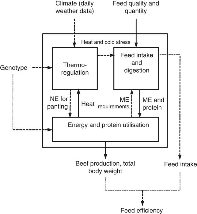
LiGAPS-Beef is based on concepts of production ecology for livestock production (Van de Ven et al., Reference Van de Ven, de Ridder, van Keulen and van Ittersum2003; Van der Linden et al., Reference Van der Linden, Oosting, Van de Ven, De Boer and Van Ittersum2015). The deterministic model integrates three sub-models that jointly simulate growth and production of a bovine animal: a thermoregulation sub-model, a feed intake and digestion sub-model, and an energy and protein utilisation sub-model (Figure 1). The defining factor genotype affects the thermoregulation sub-model and the energy and protein utilisation sub-model. The thermoregulation sub-model accounts for the effects of the defining factor climate. The feed intake and digestion sub-model accounts for effects of feed quality and quantity, which are both limiting factors. The three sub-models are interconnected by energy and protein flows within an animal (Figure 1). Energy flows distinguished are gross energy, digestible energy (DE), metabolisable energy (ME), net energy (NE) and heat. The inputs for LiGAPS-Beef are breed-specific parameters (n=22), generic parameters for cattle (n=89), physical and chemical parameters (n=24), daily weather data, feed characteristics, diet composition and feed availability. These inputs are specified in the Supplementary Material (Tables S1 to S6).
Representation of LiGAPS-Beef (Livestock simulator for Generic analysis of Animal Production Systems – Beef cattle) and the connections among the three sub-models. Solid arrows indicate flows of material or energy, dashed arrows indicate a flow of information. ME=metabolisable energy; NE=net energy.

The main outputs of LiGAPS-Beef are feed intake, beef production, total BW (TBW) and feed efficiency (FE), while the biophysical factors that define and limit growth can be derived. Defining factors are the genotype and climate (heat and cold stress), and limiting factors included in the model are feed quality and available feed quantity. Feed quality limitation occurs if the maximum capacity for feed digestion is fully utilised. Feed quantity limitation occurs if the available amount of feed is not sufficient to meet the energy or protein requirements of an animal given its genotype, the ambient climate and the feed quality. This results in either energy or protein deficiency. The time step of the model is 1 day. Animals can be simulated over their whole life span, which is potentially more than 10 years for beef cows. LiGAPS-Beef is written in the programming language R, version 2.15.3 (RCoreTeam, 2013).
Thermoregulation sub-model
The thermoregulation sub-model simulates heat release from an animal. This sub-model is based on existing thermoregulation models of McGovern and Bruce (Reference McGovern and Bruce2000) and Turnpenny et al. (Reference Turnpenny, McArthur, Clark and Wathes2000) that simulate thermoregulation within a day. These models have been adapted to simulate heat flows with a time step of one day. Inputs for the thermoregulation sub-model are breed-specific parameters, generic parameters for cattle, daily weather data, and heat production. Heat production is an output of the energy and protein utilisation sub-model (Figure 1). Daily weather data required are average temperature, solar radiation, vapour pressure, wind speed, cloudiness and precipitation. Weather data from meteorological stations are used as input if cattle are kept outdoors. Outdoor weather data are empirically converted to indoor weather data if cattle are kept in stables that are not fully closed, which is generally the case for beef cattle.
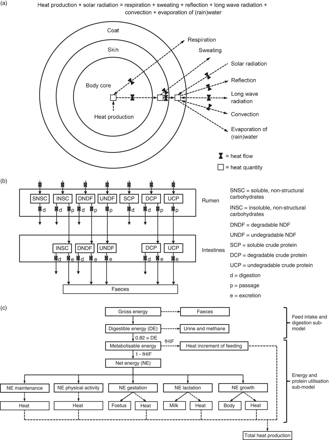
The thermoregulation sub-model represents an animal as a cylinder consisting of three layers: body core, skin and coat (Figure 2a). Cattle are isothermal animals with a body temperature of 39°C. Heat produced in the body core is released through respiration, or passed on to the skin. Heat from the skin is released as latent heat (sweating), or passed on to the coat. Heat from the coat is released through long wave radiation, convection and evaporation of rainwater. Solar radiation is partly reflected (Figure 2a). To maintain body temperature, the sum of heat production and heat load via solar radiation must equal the sum of heat release through respiration, sweating, reflection of solar radiation, long wave radiation, convection and evaporation of rainwater (McGovern and Bruce, Reference McGovern and Bruce2000; Turnpenny et al., Reference Turnpenny, McArthur, Clark and Wathes2000) (Figure 2a).
(a) Schematic overview of heat flows in beef cattle simulated with the thermoregulation sub-model. (b) Digestion of feed constituents in the rumen and intestines simulated with the feed intake and digestion sub-model, adapted from Chilibroste et al. (Reference Chilibroste, Aguilar and Garcia1997). (c) Schematic overview of energy flows in beef cattle simulated with the energy and protein utilisation sub-model. fHIF=fraction heat increment of feeding. Adapted from NRC (1981).

Cattle regulate heat release by three mechanisms: adjustment of the respiration rate, vasoconstriction or vasodilatation, and adjustment of the sweating rate. Minimum heat release is achieved at a minimum respiration rate, maximum vasoconstriction and minimum sweating rate, whereas maximum heat release is achieved at the opposites. Heat production is the balancing variable in the thermoregulation sub-model to maintain body temperature. If heat production is lower than the minimum heat release, additional energy is required to prevent a decrease in body temperature. If the genotype, feed quality and feed quantity allow the heat production from metabolic processes to exceed the maximum heat release, an animal reduces feed intake to prevent an increase in body temperature (Figure 1). If heat production is between minimum and maximum heat release, the animal is in its thermoneutral zone. The output of this sub-model is a heat balance, which indicates the additional energy requirements under cold conditions or the required reduction in heat production, and hence growth, under warm conditions.
Feed intake and digestion sub-model
Inputs for the feed intake and digestion sub-model are feed types, feed composition, fill units (FUs), available feed quantities, and energy requirements from the energy and protein utilisation sub-model. The feed intake and digestion sub-model is based on the FU system developed by the French National Institute for Agricultural Research/Institut National de la Recherche Agronomique (INRA) (Jarrige et al., Reference Jarrige, Demarquilly, Dulphy, Hoden, Robelin, Beranger, Geay, Journet, Malterre, Micol and Petit1986; INRA, 2007; Faverdin et al., Reference Faverdin, Baratte, Delagarde and Peyraud2011) and the rumen model of Chilibroste et al. (Reference Chilibroste, Aguilar and Garcia1997). Feed intake cannot exceed the maximum digestion capacity of an animal, which is proportional to its metabolic BW. The maximum digestion capacity and feed intake are expressed in FUs; 1 kg dry matter (DM) of a reference pasture grass has a FU of one, whereas other feed types have a FU relative to this reference. Feed intake is the minimum of feed intake to meet energy requirements, maximum feed intake determined by climate conditions, feed intake corresponding to the maximum rumen digestion capacity and feed availability.
The rumen model of Chilibroste et al. (Reference Chilibroste, Aguilar and Garcia1997) simulates feed digestion in the rumen. This model distinguishes seven feed constituents, whose digestion and passage in the rumen are described by first-order reactions (Figure 2b). Digestion rates differ among feed constituents, whereas passage rates are similar for all feed constituents (Chilibroste et al., Reference Chilibroste, Aguilar and Garcia1997). Passage rates increase with increasing rumen fill. We added the digestion and passage of feed constituents in the intestines to assess the total digestibility of feed in the whole digestive tract. The total feed DM that is digested corresponds to DE, whereas undigested feed DM ends up in the faeces (Figure 2b). We assumed that ME is 0.82 times DE for cattle (National Research Council (NRC), 2000).
Energy and protein utilisation sub-model
In this paper, NE is defined as energy available for maintenance, physical activity, growth, gestation and lactation (NRC, 2000). Hence, NE is not calculated as ME minus total heat production, which equals retained energy in body tissues and milk. Here, NE is calculated as ME minus heat increment of feeding (Figure 2c). Heat increment of feeding includes heat production from chewing, rumination, digestion and absorption of feed, as well as heat production from rumen fermentation. Heat increment of feeding is assumed to be a fraction of ME (Baldwin et al., Reference Baldwin, Smith, Taylor and Sharp1980), which depends on the digestibility of a feed type (Chandler, Reference Chandler1994). Protein requirements for chewing, rumination, digestion and absorption of feed are assumed to be proportional to the heat increment of feeding. Both NE and protein are partitioned over various metabolic processes. The NE for maintenance and physical activity is fully converted into heat, whereas NE for growth, gestation and lactation is converted partly into heat and partly into body tissues or milk. The sum of heat increment of feeding and heat production from metabolic processes equals the total heat production (Figure 2c).
The NE for maintenance is equal to heat production during fasting and is a function of metabolic BW (kg0.75). The NE for physical activity (i.e. grazing and locomotion) is assumed to be a function of metabolic BW under outdoor conditions, but is assumed to be negligible for cattle in feedlots and stables. Protein requirement is assumed to be 0.48 g/MJ NE (Commonwealth Scientific and Industrial Research Organisation (CSIRO), 2007) for maintenance and for physical activity. The NE and protein requirements for gestation and lactation are breed- and sex-specific (Fox et al., Reference Fox, Sniffen and O’Connor1988; Jenkins and Ferrell, Reference Jenkins and Ferrell1992; CSIRO, 2007). The genetic potential for growth is described by the derivative of breed- and sex-specific Gompertz curves, which apply if no other factors than the genotype are affecting growth (i.e. if sufficient NE and protein are available for growth). Body tissues distinguished are non-carcass tissue and carcass tissues. The latter consist of bone tissue, muscle tissue and fat tissue (intramuscular fat, intermuscular fat and subcutaneous fat). Beef is defined as deboned carcass. Each body tissue consists of protein, lipid, ash and water, from which only protein (44 kJ/g) and lipid (54 kJ/g) accretion require NE (Emmans, Reference Emmans1994). The daily NE requirement for growth is calculated subsequently as the amount of protein and lipid accreted in all body tissues times the NE requirements for protein and lipid accretion. Likewise, the daily protein requirement for growth is calculated as the amount of protein accreted in body tissues times the efficiency for protein accretion (54%). Rumen contents are a fixed fraction of the TBW, and do not require NE and protein for growth.
The NE and protein for growth are balancing variables, whereas the other metabolic processes are fully sustained. If heat production from metabolic processes and heat load from solar radiation is below minimum heat release, additional NE and protein is required (Figure 1), which can reduce NE and protein availability for growth. Body tissues are not affected equally by sub-optimal supply of NE (Hornick et al., Reference Hornick, Van Eenaeme, Gerard, Dufrasne and Istasse2000). Growth reductions affect the non-carcass tissue least and the fat tissue in the carcass most. Compensatory growth can occur after a period of growth retardation (Hornick et al., Reference Hornick, Van Eenaeme, Gerard, Dufrasne and Istasse2000). LiGAPS-Beef simulates compensatory growth if climatic conditions are favourable and if adequate amounts of NE and protein are available for growth.
Upscaling from the animal to herd level
Meeting the global demand for food requires an increase in agricultural production per unit of land (Van Ittersum et al., Reference Van Ittersum, Cassman, Grassini, Wolf, Tittonell and Hochman2013). Beef production per hectare can be calculated as the FE of a herd (kg beef/ton DM feed) multiplied by the weighted average yield of feed crops (t DM feed/ha per year) (Van der Linden et al., Reference Van der Linden, Oosting, Van de Ven, De Boer and Van Ittersum2015). LiGAPS-Beef simulates the performance of one animal, so upscaling to the herd level is required to simulate beef production systems. A beef herd can be subdivided in productive animals (calves raised for beef) and reproductive animals. The reproductive herd generally accounts for approximately 70% of the feed intake, but its contribution to beef production is much lower (De Vries et al., Reference De Vries, van Middelaar and de Boer2015). Hence, assessing potential and feed-limited production for beef herds requires the inclusion of both the productive and the reproductive herd.
The smallest herd possible includes one reproductive cow. This cow must be replaced by a heifer at the end of her lifetime to maintain the production of calves. Hence, the smallest possible herd consists of one cow and all its offspring produced during her lifetime, minus a replacement heifer. This smallest possible herd is defined as a herd unit. A herd in a beef production system consists of multiple herd units (Van der Linden et al., Reference Van der Linden, Oosting, Van de Ven, De Boer and Van Ittersum2015). Each animal in the herd unit is simulated over its complete life cycle. Reproductive bulls are assumed to be negligible in a herd unit, as the ratio of cows to bulls is generally high. The FE of a herd unit can be used to assess the potential and feed-limited beef production per unit agricultural area used for production of feed crops.
Potential and feed-limited production
Potential production of livestock is achieved if only the genotype and climate affect growth (Van de Ven et al., Reference Van de Ven, de Ridder, van Keulen and van Ittersum2003; Van der Linden et al., Reference Van der Linden, Oosting, Van de Ven, De Boer and Van Ittersum2015). Feed is provided ad libitum under potential production, since the feed quantity available is, by definition, not limiting for growth. Feed quality is sufficient to meet NE and protein requirements under potential production. In addition, the diet should contain sufficient fibrous material to sustain rumen functioning. The diet under feed-limited production corresponds to the diet fed in practice (Van de Ven et al., Reference Van de Ven, de Ridder, van Keulen and van Ittersum2003; Van der Linden et al., Reference Van der Linden, Oosting, Van de Ven, De Boer and Van Ittersum2015). Potential and feed-limited production are achieved under ideal management (Van de Ven et al., Reference Van de Ven, de Ridder, van Keulen and van Ittersum2003). Management decisions, such as culling rates and slaughter weights, determine the FE of a herd unit (Van der Linden et al., Reference Van der Linden, Oosting, Van de Ven, De Boer and Van Ittersum2015). With adequate diets and ideal management, cows generally calve for the first time in their 3rd year. Assuming a maximum conception age of 10 years and a minimum calving interval of 1 year, cows can produce up to eight calves during their lifetime. For beef cattle, the FE of a herd unit is theoretically at its maximum if the culling rate of cows is 50% per year after birth of the first calf (Van der Linden et al., Reference Van der Linden, Oosting, Van de Ven, De Boer and Van Ittersum2015). This high culling rate is explained first by the higher FE of primiparous cows, which produce calves and increase their TBW simultaneously. The fraction of primiparous cows in a herd increases with an increasing culling rate. In addition, primiparous cows have lower TBWs than multiparous cows, which reduces their maintenance requirements and subsequently increases their FE.
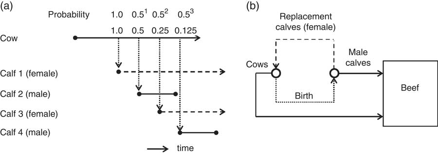
A culling rate of 50% per year after birth of the first calf implies that cows give birth to one calf in their 3rd year, on average 0.5 (0.51) calves in their 4th year, 0.25 (0.52) calves in their 5th year and so on, up to 0.008 (0.57) calves in their 10th year (Figure 3a). In total, approximately two calves are obtained per cow and per herd unit on average (1+0.51+0.52+ … + 0.57≈2). One of these calves is a male calf, and one a female calf for replacement, assuming a male to female ratio of one (Van der Linden et al., Reference Van der Linden, Oosting, Van de Ven, De Boer and Van Ittersum2015). The replacement calf gives rise to the next herd unit. One herd unit thus consists of one reproductive cow, and one male calf (Van der Linden et al., Reference Van der Linden, Oosting, Van de Ven, De Boer and Van Ittersum2015). Hence, all female calves are used as replacement calves, and male calves are raised for beef production (Figure 3b). In addition, the slaughter weight of the male calf in a herd unit must be optimised to maximise FE of the herd unit.
(a) Life spans of a cow and male calves in a herd unit (solid lines). Replacement calves (dashed lines) are not part of the herd unit. Dotted lines indicate birth. Male and female calves are in random order, and only four out of the maximum of eight calves per cow are indicated. (b) Herd dynamics under potential and feed-limited production. Solid lines indicate beef production, the dashed line indicates replacement, and the dotted line birth. Adapted from Van der Linden et al. (Reference Van der Linden, Oosting, Van de Ven, De Boer and Van Ittersum2015).

Model illustration at the animal and herd level
LiGAPS-Beef was illustrated at the animal and herd level for 10 hypothetical cases. Charolais and B×S cattle were simulated under potential and feed quality limited production in France and Australia, which resulted in eight cases (Table 1). For potential production, finding the ideal daily composition of feed for each animal in a herd unit is complicated. We propose, therefore, that the diet under potential production is fixed for all animals in a herd unit, contains sufficient fibre and consists of high-quality feeds. An ad libitum diet consisting of 65% wheat and 35% high-quality hay is assumed to closely meet these requirements (Van der Linden et al., Reference Van der Linden, Oosting, Van de Ven, De Boer and Van Ittersum2015). The ME content of this diet (11.6 MJ ME/kg DM) is relatively high, the FU value (0.76 kg-1 DM) is relatively low, and it is available in many countries worldwide. This fixed diet facilitates comparison of FE in different beef production systems under potential production.
Cases with potential and feed-limited production levels of beef cattle to illustrate LiGAPS-Beef (Livestock simulator for Generic analysis of Animal Production Systems – Beef cattle) at the animal and herd level

Pot=potential production; Ch=Charolais; Fr=France; Au=Australia; B×S=¾ Brahman × ¼ Shorthorn cattle; FQlty=feed quality limited production; FLim=feed-limited production; DM=dry matter; TBW=total BW.
1 Housed indoors from December to March.
2 Hay fed indoors (December to March), grazing outdoors (April to November).
3 Barley is max. 65% of the diet, or 1 kg DM/day. The remaining part of the diet is from hay (December to March) and grass (April to November).
4 Feed quantity available is 2% of the total BW of the animal.
Under feed quality limitation, 95% of the diet was grass-based, and 5% consisted of barley in both countries. The ninth case included a diet with 1 kg DM barley per head per day, and the remainder was grass-based. The 10th case included the grass-based diet with 5% barley, but the amount of feed available was at most 2% of the TBW (Table 1). Weather data for France were from Charolles (46.4°N, 4.3°E), and for Australia from Kununurra (15.7°S, 128.7°E). Cattle in France were kept indoors from December to March, and outdoors from April to November. Cattle were grazing on pasture when kept outdoors (8.8 MJ ME/kg DM), and were fed hay when kept indoors (9.6 MJ ME/kg DM). Cattle in Australia were kept outdoors year-round on pasture (8.8 MJ ME/kg DM). For simplicity, the quality of wheat, barley, grass and hay was fixed over time. The age at weaning was set at 210 days in both countries. Energy requirements for physical activity were calculated from metabolic BWs (70 kJ/kg0.75) (CSIRO, 2007).
The 10 cases were illustrated first at the animal level, where a single bull calf was simulated. Charolais and B×S bull calves were slaughtered at a weight of 500 kg TBW in the hypothetical cases. Next, the 10 cases were illustrated at the herd level. As described before, a herd unit consists of one reproductive cow and one bull calf. The culling rate was 50% after birth of the first calf, and the slaughter weight of the bull (calf) was optimised to maximise the FE of the herd unit. The slaughter weight was optimised by simulating the FE at the herd level for a range of TBWs at slaughter (step-wise procedure). Subsequently, a quadratic function was fitted to the FE at the herd level and the slaughter weights, where the maximum FE obtained from this function corresponds with the optimum slaughter weight.
Results
Model illustration at the animal level
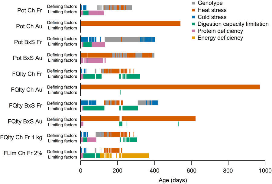
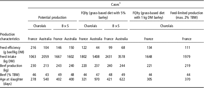
Individual Charolais bulls had a higher FE in France than in Australia, both under potential and feed-limited production (Table 2). Charolais bulls had higher FEs than B×S bulls in France, and B×S bulls had higher FEs than Charolais bulls in Australia (Table 2). Charolais bulls fed with a grass-based diet up to 2% of the TBW had a 9% lower FE compared with ad libitum supply of the same diet (111 and 122 g beef/kg DM), which is fully attributed to feed quantity limitation. Differences in FE among the cases were mainly attributed to differences in feed intake, as bulls were slaughtered at 500 kg TBW, which resulted in a similar beef production levels (kg per animal) and similar percentages of beef in the TBW. An increased feed intake was associated with an increasing age at slaughter (Table 2). LiGAPS-Beef simulated the factors that define and limit growth for each of the 10 cases (Figure 4). For the cases in France, cold stress occurred during winter and heat stress during summer. For the cases in Australia, heat stress was a major defining factor. Under potential production, growth of both cattle breeds was influenced by minor protein deficiencies and limitation in digestion capacity before weaning, except for Charolais bulls in Australia (Figure 4). Limitation in digestion capacity influenced growth when ad libitum grass-based diets were fed to bulls. Protein deficiency was did not limiting growth in any of the cases after weaning, whereas energy deficiency occurred also after weaning when the feed quantity available was at most 2% of the TBW (Figure 4).
Defining and limiting factors for growth and feed efficiency of bulls in the 10 cases (see Table 1) at the animal level. Digestion capacity limitation of the cattle is caused by feed quality limitation. Protein deficiency can be caused by feed quality and quantity limitation. Energy deficiency is caused by feed quantity limitation only. Pot=potential production; Ch=Charolais; Fr=France; Au=Australia; B×S=¾ Brahman × ¼ Shorthorn cattle; FQlty=feed quality limited production; FLim=feed-limited production.

Feed efficiency, feed intake, beef production and age of slaughter of cattle in the 10 cases (see Table 1) used to illustrate LiGAPS-Beef (Livestock simulator for Generic analysis of Animal Production Systems – Beef cattle) at the animal level

Bulls are slaughtered at 500 kg total BW (TBW).
FQlty=feed quality limited production; DM=dry matter; B×S=¾ Brahman× ¼ Shorthorn cattle.
1 See Table 1 for explanation on the cases.
Model illustration at the herd level
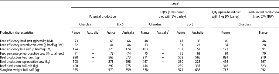
Beef production at the herd level was assessed by using the concept of the herd unit. LiGAPS-Beef did not yield results for Charolais cattle in Australia, because heat stress in Australia resulted in mortality of reproductive Charolais cows (Table 3). The FE at the herd level was based on the FE of the reproductive cow and the FE of one bull calf (Table 3). The FE at the herd level was higher for Charolais than for B×S cattle under potential production in France, whereas the FE was similar under feed quality limited production in France (Table 3). In most cases, the percentage feed consumed by the reproductive cow in a herd was approximately 70% of the total feed for the herd unit. Reproductive cows accounted, however, for 84% of feed intake of the herd unit when barley was fed at 1 kg/head per day (Table 3).
Beef production, feed intake and feed efficiency of cattle in the 10 cases (Table 1) used to illustrate LiGAPS-Beef (Livestock simulator for Generic analysis of Animal Production Systems – Beef cattle) at the herd level

FQlty=feed quality limited production; DM=dry matter; TBW=total BW; B×S=¾ Brahman× ¼ Shorthorn cattle.
1 See Table 1 for explanation on the cases.
2 No results due to inability of reproductive cows to cope with heat stress.
Discussion
Model description and upscaling to the herd level
We integrated sub-models on thermoregulation, feed intake and digestion, and energy and protein utilisation to account for the interactions among the genotype, climate, feed quality and quantity on beef production (Figure 1). Such four-way interactions cannot be simulated with the individual sub-models that were based on existing models. For example, the mechanistic thermoregulation models used in LiGAPS-Beef simulate heat flows, but no ME and NE flows for processes such as growth (McGovern and Bruce, Reference McGovern and Bruce2000; Turnpenny et al., Reference Turnpenny, McArthur, Clark and Wathes2000). The existing livestock models and frameworks used to simulate energy and protein utilisation include ME and NE flows, but do not consider heat flows, or thermoregulation is included empirically (NRC, 2000; CSIRO, 2007). In addition, our feed intake and digestion sub-model was largely based on an existing feed digestion model, which does not account for energy demands or effects of the climate (Chilibroste et al., Reference Chilibroste, Aguilar and Garcia1997). Input from the energy and protein utilisation sub-model and the thermoregulation model was required, therefore, to simulate feed intake (Figure 1). Hence, the quantification of potential and feed-limited beef production and the identification of the factors that define and limit growth are novel features (i.e. emergent properties) of LiGAPS-Beef that result from the integration of sub-models.
Next, we discuss some of the methodological choices during the development of LiGAPS-Beef and the corresponding limitations of the model. First, the thermoregulation models used as a basis for the thermoregulation sub-model simulate heat release throughout the day, but the thermoregulation sub-model itself has a time step of one day, just like the other two sub-models. Despite the larger time step, and consequently a loss of detail, the thermoregulation sub-model simulated heat release fairly well, and live weight gain was simulated fairly well for cattle in different climates (Van der Linden et al., Reference Van der Linden, Van de Ven, Oosting, Van Ittersum and De Boer2018a and Reference Van der Linden, Van de Ven, Oosting, Van Ittersum and De Boer2018b). Second, our model is deterministic, which implies that all animals belonging to a breed have exactly the same genotype. In reality, genetic variance within breeds can result in differences in performance among animals. Third, our model does not account for interactions between animals or herd units, whereas such interactions can occur under conditions where animals compete for feed. Fourth, we assumed single calves to be born. Although the probability of having twins and triplets is relatively low in cattle, the FE at the herd level may be slightly underestimated by not accounting for twins and triplets. Fifth, we assumed that cow parity does not significantly affect birth weight, milk production and calf performance. In practice, firstborn calves may have lower birth weights and performance, which could reduce FE of herds, especially if culling rates are high. Sixth, the limiting factor drinking water was not taken into account in LiGAPS-Beef, since we assumed that cattle are seldom deprived from water. Deficiencies of minerals and vitamins were not accounted for either. Feed-limited production may thus be overestimated in case drinking water, minerals or vitamins are limiting cattle growth and production. Finally, LiGAPS-Beef focusses on beef cattle at the animal and herd level, and does not include the crop or grassland component of farming systems. Connecting the livestock and crop or grassland component of a farming system is relevant for feed budgeting, especially in grazing systems where strong interactions between animals and the sward exist. For this reason, LiGAPS-Beef was connected elsewhere to a grass growth model to simulate grass-based beef production in the Charolais region of France (Van der Linden et al., Reference Van der Linden, Oosting, Van de Ven, Veysset, de Boer and Van Ittersum2018c).
Model illustration at the animal level
Simulation results show that Charolais bulls had the highest FE in France, and B×S bulls had the highest FE in Australia (Table 2). Hence, the breed adapted to a region and its prevailing climate conditions has a higher FE than the less-adapted breed, which is in line with literature (Burrow, Reference Burrow2012). The FE of Charolais bulls under potential production in France (216 g beef/kg DM) resembled the FE of Charolais bulls (171 g beef/kg DM) fed a similar diet in Germany, although these bulls were slaughtered at a later age (Pfuhl et al., Reference Pfuhl, Bellmann, Kuhn, Teuscher, Ender and Wegner2007). LiGAPS-Beef identified the factors that define and limit growth under potential and feed-limited production (Figure 4). Occurrence of cold stress in winter and heat stress in summer in France and occurrence of heat stress in Australia is in line with the expectations. As expected, limiting feed intake to 2% of the TBW resulted in energy deficiency and a reduced growth (Table 2, Figure 4). All in all, the production levels and the corresponding biophysical factors identified were corresponding reasonably to expectations and literature.
It should be noted that digestion capacity limitation and protein deficiency influenced growth under potential production before weaning (Figure 4). This implies that the diet consisting of 65% wheat and 35% hay (Van der Linden et al., Reference Van der Linden, Oosting, Van de Ven, De Boer and Van Ittersum2015) was not entirely adequate to achieve potential production. Feeding other diets, however, did not result in complete elimination of these factors either. Digestion capacity limitation and protein deficiency occurred before weaning, when the rumen shifts from a milk-based diet to a diet consisting of solid feed. This shift is affected by the animals genotype, so it might be justified to assume that potential production is achieved with the diet consisting of 65% wheat and 35% hay.
Model illustration at the herd level
The FE of Charolais cattle at the herd level was highest in France, but reproductive cows did not perform in Australia due to heat stress (Table 3). This matches with literature indicating that Bos taurus cattle perform better in temperate climates than in tropical climates (Burrow, Reference Burrow2012). To our knowledge, no literature is available on mortality of Charolais or other large-sized B. taurus cattle due to heat stress in northern Australia, since the breeds used in this region are generally crossbreds between Bos indicus and B. taurus cattle. Simulation results showed that Charolais cattle had the highest FE in France under potential production, and B×S herds in Australia (Table 3). Hence, the breed adapted to a region and its prevailing climate conditions has a higher FE in this region than the less-adapted breed, which is in line with literature (Burrow, Reference Burrow2012).
The percentage of feed supplied to reproductive cows in a herd was generally between 70% and 75% of the total feed supply (Table 3). This is in agreement with de Vries et al. (Reference De Vries, van Middelaar and de Boer2015), who stated that reproductive cows account for 70% of the total feed intake at the herd level. Reproductive cows required 84% of the feed when the quantity of barley was fixed at 1 kg/head per day (Table 3). This feeding strategy decreases the proportion of barley in the diet over the lifetime of an animal. Diets of calves are expected, therefore, to have higher wheat contents than diets of reproductive cows. Due to the high ME content of barley, bull calves could suffice with lower amounts of feed than reproductive cows, which results in a higher percentage of feed consumed by reproductive cows.
In line with its objective, LiGAPS-Beef simulated potential and feed-limited production in different beef production systems (Tables 2 and 3), and identified the factors that define and limit growth (Figure 4). To our knowledge, LiGAPS-Beef is the first livestock model that explicitly indicates which biophysical factor defines or limits growth and production during which period. Identification of these factors is a crucial step in yield gap analysis, and a starting point to list improvement options to mitigate yield gaps (Van Ittersum et al., Reference Van Ittersum, Cassman, Grassini, Wolf, Tittonell and Hochman2013). Before using LiGAPS-Beef for yield gap analysis, sensitivity analyses should be conducted to get insight in the parameters affecting its output most. In addition, model evaluation with experimental data is required to get insight in the accuracy of the model when simulating beef production in contrasting systems. Results of these sensitivity analyses and model evaluations are presented in companion papers (Van der Linden et al., Reference Van der Linden, Van de Ven, Oosting, Van Ittersum and De Boer2018a and Reference Van der Linden, Van de Ven, Oosting, Van Ittersum and De Boer2018b).
Conclusions
This paper describes LiGAPS-Beef, a mechanistic model simulating beef cattle based on concepts of production ecology. LiGAPS-Beef aims to simulate potential and feed-limited production of cattle in different beef production systems, and to identify the factors that define and limit growth. A major innovation of the model is the simulation of interactions among cattle genotype, climate, feed quality and available feed quantity, by integration of sub-models for thermoregulation, feed intake and digestion, and energy and protein utilisation. LiGAPS-Beef was illustrated with simulations for different genotypes (Charolais and B×S breeds), climates (France and Australia) and feeding strategies. Model illustration suggests that the potential and feed-limited production are generally in line with literature and expectations, as well as the biophysical factors for growth that were identified. Simulations indicate that breeds adapted to a region and its climate conditions achieve a higher FE in such a region than less-adapted breeds. In conclusion, LiGAPS-Beef complied with the aim it was developed for. The model may be used, therefore, as a tool to assess and analyse yield gaps in beef production systems after conducting sensitivity analyses and model evaluation with independent experimental data.
Acknowledgements
This research is part of the Wageningen University & Research strategic programme ‘Mapping for sustainable intensification’, 2012-2016, funded by the strategic funds of Wageningen University & Research, and the PE&RC and WIAS graduate schools of Wageningen University.
Declaration of interest
The authors declare they have no conflicts of interest.
Ethics statement
None.
Software and data repository resources
The source code of LiGAPS-Beef is freely accessible at https://doi.org/10.18174/442973 and the model portal of the Plant Production Systems group of Wageningen University, The Netherlands (http://models.pps.wur.nl/content/ligaps-beef). Updates and model applications will be published on the model portal.
Supplementary material
To view supplementary material for this article, please visit https://doi.org/10.1017/S1751731118001726