1 Introduction
Vortex rings are ubiquitous in classical fluid mechanics. They are central to many natural and artificial fluid dynamic processes (Hill Reference Hill1975; Dengler & Reeder Reference Dengler and Reeder1997; Spalart Reference Spalart1998; Emanuel Reference Emanuel2005; Smith, Montgomery & Zhu Reference Smith, Montgomery and Zhu2005). Vortices are formed due to various mechanisms that span disparate physical domains (Rayfield & Reif Reference Rayfield and Reif1964; Thomson & Newall Reference Thomson and Newall1885; Dahm, Scheil & Tryggvason Reference Dahm, Scheil and Tryggvason1989; Lee et al. Reference Lee, Park, Lee, Weon, Fezzaa and Je2015; Manu et al. Reference Manu, Anand, Chetia and Basu2015). In addition to the above, the study of vortex rings has attracted many researchers due to their notable existence, at different spatiotemporal scales, in fluid flow (She, Jackson & Orszag Reference She, Jackson and Orszag1990; Pullin & Saffman Reference Pullin and Saffman1998).
Vortex interactions have also been found to play a major role in various fluid dynamic and heat transfer processes. Once formed, vortex rings are self-sustained and self-propelled. Propulsive features are characteristic to vortex shedding and resultant coherent structures (Turner Reference Turner1960; Fohl Reference Fohl1967; Spedding, Hedenström & Rosén Reference Spedding, Hedenström and Rosén2003; Dabiri & Gharib Reference Dabiri and Gharib2005). Thus, vortex shedding has been found of significance in a variety of engineering applications (e.g. transportation, flow control) as well as in biological systems (e.g. fish swimming and insect flight) (Moore & Saffman Reference Moore and Saffman1973; Weihs Reference Weihs1973; Lugt Reference Lugt1983; Dabiri Reference Dabiri2009). A number of studies (Gharib et al. Reference Gharib, Rambod, Kheradvar, Sahn and Dabiri2006; Arvidsson et al. Reference Arvidsson, Kovács, Töger, Borgquist, Heiberg, Carlsson and Arheden2016) have also highlighted the importance of vortical flows for the diagnosis of various ailments.
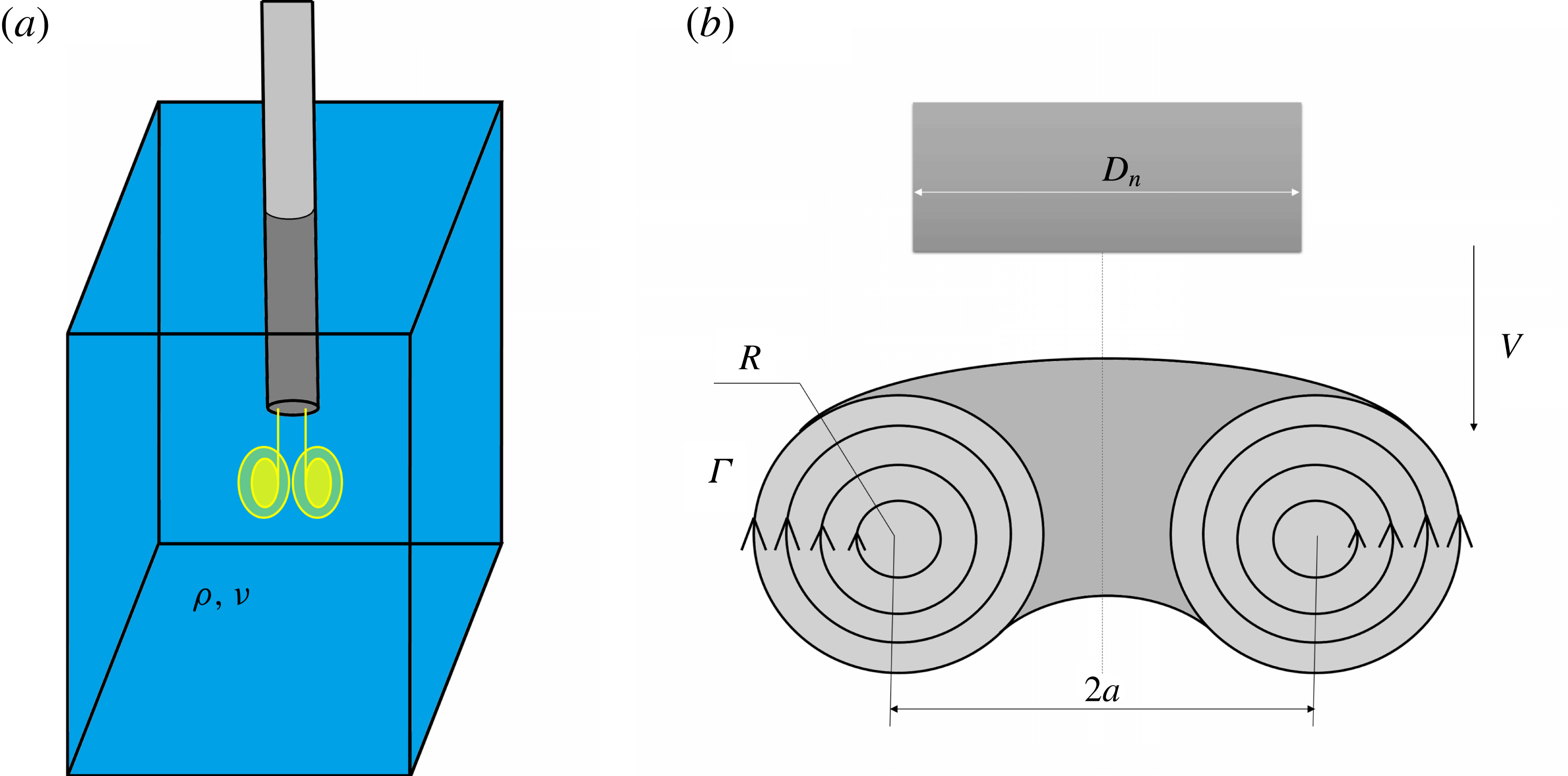
Schematic of vortex ring generation and vortex parameters.

Laboratory experiments on vortex rings are usually performed to understand vortex formation, evolution, interaction and decay. Vortices are usually formed by forcing bulk fluid through a constricted opening such as an orifice or a nozzle. Recent studies by Gharib, Rambod & Shariff (Reference Gharib, Rambod and Shariff1998) showed that there is a maximum cap on the circulation that can be induced by a single vortex ring. According to this study, a single vortex is obtained for values of
 $L/D_{n}<4$
, where
 $L$
is the stroke length and
 $D_{n}$
is the internal nozzle diameter. The concept of the formation number (FN;
 $L/D_{n}$
) can be effectively extended to other experimental configurations as well.
Analytical studies concerning vortex ring evolution can be traced back to the work of Helmholtz (Reference Helmholtz1858) and Kelvin (Reference Kelvin1867). Early theoretical studies on the formation and evolution of vortex rings (assuming inviscid behaviour) were conducted by Lamb (Reference Lamb1932) and Sommerfeld (Reference Sommerfeld1950). Studies show that a fully developed axisymmetric vortex is governed by two parameters, namely the vorticity distribution and the toroidal radius, as shown in figure 1. Dyson (Reference Dyson1893) and Fraenkel (Reference Fraenkel1972), through rigorous mathematical formulations, coined expressions for the translational velocity of inviscid thin vortex rings.
Detailed studies of vortex translation in viscous fluid were conducted by Saffman (Reference Saffman1970) and Pullin (Reference Pullin1979), where they assumed a vorticity distribution as given by Lamb–Oseen (1.1)
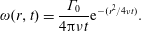 $$\begin{eqnarray}\unicode[STIX]{x1D714}(r,t)=\frac{\unicode[STIX]{x1D6E4}_{0}}{4\unicode[STIX]{x03C0}\unicode[STIX]{x1D708}t}\text{e}^{-(r^{2}/4\unicode[STIX]{x1D708}t)}.\end{eqnarray}$$
Here,
 $\unicode[STIX]{x1D6E4}_{0}$
stands for initial circulation while
 $\unicode[STIX]{x1D714},\unicode[STIX]{x1D708},r$
and
 $t$
represent the vorticity distribution, kinematic viscosity of the fluid, radial distance from the core centre and time, respectively. Using this, Saffman also derived the vortex propagation velocity to the first order, given by
 $$\begin{eqnarray}V=\frac{\unicode[STIX]{x1D6E4}_{0}}{4\unicode[STIX]{x03C0}a_{0}}\left[\ln \left(\frac{8a_{0}}{\sqrt{4\unicode[STIX]{x1D708}t}}\right)-0.558+O\left\{\left(\frac{\unicode[STIX]{x1D708}t}{a_{0}^{2}}\right)^{1/2}\ln \left(\frac{\unicode[STIX]{x1D708}t}{a_{0}^{2}}\right)\right\}\right],\end{eqnarray}$$
where the expression for the Saffman core radius is given by
 $r_{cs}=\sqrt{4\unicode[STIX]{x1D708}t}$
. These equations are valid for finite core sizes in viscous fluids for small time values, typically for
 $t\,\ll \,T$
, where
 $T$
is the piston stroke time. The above results were derived considering (1.1), for which circulation turns out to be
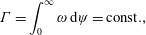 $$\begin{eqnarray}\unicode[STIX]{x1D6E4}=\int _{0}^{\infty }\unicode[STIX]{x1D714}\,\text{d}\unicode[STIX]{x1D713}=\text{const}.,\end{eqnarray}$$
where
 $\unicode[STIX]{x1D713}$
stands for the area of selected contour. Thus, constant circulation, when coupled with the concept of a constant hydrodynamic impulse, mandates that the vortex ring diameter should remain invariant in time. Thus, the thin-core model proposed by Saffman could not account for the decreasing circulation or ring expansion as observed in the experiments. However, using an order of magnitude argument, Saffman proposed relations for the translational velocity
 $V$
and radius
 $a$
for thick rings at longer times:
 $$\begin{eqnarray}\displaystyle & \displaystyle a^{2}\approx a_{0}^{2}+k^{\prime }\unicode[STIX]{x1D708}t & \displaystyle\end{eqnarray}$$
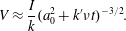 $$\begin{eqnarray}\displaystyle & \displaystyle V\approx \frac{I}{k}(a_{0}^{2}+k^{\prime }\unicode[STIX]{x1D708}t)^{-3/2}. & \displaystyle\end{eqnarray}$$
Here,
 $I$
stands for the impulse of the vortex ring and
 $k$
and (
 $k^{\prime }$
) are constants. This aspect was further explored by Maxworthy (Reference Maxworthy1972, Reference Maxworthy1977), where he performed multiple experiments on laminar vortex rings
 $(Re<600)$
. He reported overprediction in the ring expansion as given by (1.4). Using his entrainment model, he tried to explain the changes in vortex parameters and provided relations for vortex size, circulation and convective velocity:
 $$\begin{eqnarray}a\propto t^{1/3},\quad \unicode[STIX]{x1D6E4}\propto t^{-2/3},\quad V\propto t^{-1}.\end{eqnarray}$$
Maxworthy arrived at these empirical relations using scaling arguments and dimensional analysis. This subject was later addressed by the work of Cantwell & Rott (Reference Cantwell and Rott1988), Stanaway, Cantwell & Spalart (Reference Stanaway, Cantwell and Spalart1988) and Fukumoto & Moffatt (Reference Fukumoto and Moffatt2000) using numerical methods. These findings found corroboration with some of the existing theories. However, their model still lacked universal applicability and could not explain the dynamics for a wide range of Reynolds numbers. These studies thus show the lack of consensus among the proposed theories.
The above-mentioned vortex parameters, though intuitively complex, greatly influence vortex interactions with thermal and density stratifications ubiquitous in nature (Linden Reference Linden1973; Dahm et al. Reference Dahm, Scheil and Tryggvason1989; Orlandi, Egermann & Hopfinger Reference Orlandi, Egermann and Hopfinger1998; Advaith et al. Reference Advaith, Manu, Tinaikar, Chetia and Basu2017). Though the significance of these variables has been long known, there have been only a very limited number of studies incorporating their effects. The major reason for this lack of attention is the complex nature of vortex evolution. Recently, many analytical and numerical studies pertaining to vortex evolution have succeeded in arriving at a near accurate estimation of the vortex parameters (Bergdorf, Koumoutsakos & Leonard Reference Bergdorf, Koumoutsakos and Leonard2007). However, these equations are either mathematically complex or iterative, and hence provide limited physical insights into phenomena such as vortex interactions.
A detailed review of available theories and their results are included in supplementary material available at https://doi.org/10.1017/jfm.2017.815. In summary, most of the analytical studies on vortex evolution have focused on the asymptotic behaviours of its lifetime. At the lower end, studies have been conducted for thin vortex rings using the classical vorticity equation of Lamb–Oseen (1.1). At the other end, almost all the studies resort to conservation of hydrodynamic impulse to arrive at the long-time behaviour. These two extreme approaches are, however, fundamentally different from each other. Rarely there have been efforts to link the two. Moreover, any attempts in this direction have been unfruitful, and thus the transformation of short-time equations into the long-time regime is a problem, still unresolved. In addition, many different forms of viscous time scales have been used throughout the literature. Parameters such as circulation (
 $\unicode[STIX]{x1D6E4}$
), viscosity (
 $\unicode[STIX]{x1D708}$
), ring radius (
 $a$
) and nozzle diameter (
 $D_{n}$
) have been used casually and interchangeably, primarily aimed at normalization, with minimal insights. Thus, the available time scales are far from universal and do not successfully explain vortex evolution.
Here we try to comprehend the mechanism of vortex evolution in viscous fluids using a simple mathematical framework. This paper is divided into five sections, with § 1 being the introduction. In § 2, we try to frame simple approximated mathematical equations describing each parameter of the vortex rings. We will also try to give physical insights into vorticity diffusion and ring expansion. Details about the experimental set-up, visualization techniques and test cases will be described in § 3. In § 4, we provide the results of our experimental studies. These datasets will be compared with our theoretical predictions and results already available in the literature. Discussions about the results, including their range of validity, will be conducted in § 5. In § 6, we will summarize our study and discuss its implications.
2 Mathematical formulation
Vortex rings are formed in lab settings by impulsive ejection of fluid through a nozzle opening, as shown in figure 1. The ejected fluid rolls up to form vortex rings (Didden Reference Didden1979; Auerbach Reference Auerbach1988). During the initial period, vortex rings are unstable, with continuous momentum addition and significant viscous effects. We define this period as ‘formation time’, within which the vortex parameters are governed by initial operating conditions such as stroke length
 $L$
, transient velocity and nozzle geometry. It should be noted that this definition is not to be confused with the terminology defined by Gharib et al. (Reference Gharib, Rambod and Shariff1998), where he defined formation time
 $(L/D_{n})$
as the maximum stroke time permitted for evolution of a single vortex ring. Some basic observations describing vortex formation are elucidated in § 4.1.
Beyond ‘formation time’, the vortex ring stabilizes and attains a smooth vorticity distribution. These vortex rings then move with a self-induced velocity. For inviscid fluids, (after neglecting any instabilities) the vortex does not diffuse, resulting in a consistent vorticity distribution throughout its period of propagation. However, for real fluids with finite viscosity, diffusion gives rise to time-variant vorticity fields. This varying vorticity can be best understood by examining the vorticity transport equation given by
 $$\begin{eqnarray}\frac{\text{D}\unicode[STIX]{x1D714}}{\text{D}t}=(\unicode[STIX]{x1D714}\boldsymbol{\cdot }\unicode[STIX]{x1D735})u-\frac{\unicode[STIX]{x1D735}\unicode[STIX]{x1D70C}}{\unicode[STIX]{x1D70C}}\times \frac{\text{D}u}{\text{D}t}-g\frac{\unicode[STIX]{x1D735}\unicode[STIX]{x1D70C}}{\unicode[STIX]{x1D70C}}\times \,\boldsymbol{j}+\unicode[STIX]{x1D708}\unicode[STIX]{x1D6FB}^{2}\unicode[STIX]{x1D714}.\end{eqnarray}$$
In the above,
 $\boldsymbol{j}$
denotes a unit vector in the vertical direction while the other variables carry their usual meaning. The first term on the right denotes the vortex turning and stretching term, while the last term of the equation captures vorticity generation due to diffusion. The second and third terms on the right-hand side characterize the baroclinic generation of vorticity due to hydrostatic and hydrodynamic forces. These baroclinic vorticity terms reduce to zero for the constant-density fluid domain. Similarly, the vortex turning and stretching terms vanish for two-dimensional (2D) flows.
Even though vortex rings are three-dimensional structures, most of the insights into vortex evolution can be obtained by neglecting the curvature effects and treating 2D viscous diffusion as the dominant mechanism (Oseen Reference Oseen1910; Lamb Reference Lamb1932). Thus, a 2D axisymmetric vortex pair descending in a homogeneous incompressible fluid can be defined by (2.2), where the effects of convective velocity on vortex deformation are neglected. The vorticity transport can then be modelled in polar coordinates as a simple diffusion equation:
 $$\begin{eqnarray}\frac{\unicode[STIX]{x2202}\unicode[STIX]{x1D714}}{\unicode[STIX]{x2202}t}=\unicode[STIX]{x1D708}\unicode[STIX]{x1D6FB}^{2}\unicode[STIX]{x1D714}=\unicode[STIX]{x1D708}\left(\frac{\unicode[STIX]{x2202}^{2}\unicode[STIX]{x1D714}}{\unicode[STIX]{x2202}r^{2}}+\frac{1}{r}\frac{\unicode[STIX]{x2202}\unicode[STIX]{x1D714}}{\unicode[STIX]{x2202}r}\right).\end{eqnarray}$$
The standard procedure for solving the above equation involves the concept of similarity variables, where the implicit variables
 $r$
and
 $t$
are interlinked using a new variable
 $\unicode[STIX]{x1D702}$
. The solution yields a pure tangential velocity field. Therefore, this explicit Gaussian profile forms the solution of the complete vorticity equation rather than just its linear approximation.
 $$\begin{eqnarray}\unicode[STIX]{x1D714}(r,t)=\unicode[STIX]{x1D714}_{m}(t)\text{e}^{-(r/\unicode[STIX]{x1D70E}(t))^{2}}.\end{eqnarray}$$
2.1 Limitations of the short-time, self-similarity solution
The solution to vorticity diffusion (2.2) using self-similarity variables results in the Lamb–Oseen equation given by
 $$\begin{eqnarray}\unicode[STIX]{x1D714}(r,t)=\frac{\unicode[STIX]{x1D6E4}_{0}}{4\unicode[STIX]{x03C0}\unicode[STIX]{x1D708}t}\text{e}^{-(r^{2}/4\unicode[STIX]{x1D708}t)}\end{eqnarray}$$
This solution is obtained on the premise of the idealized condition of a highly localized initial vorticity distribution given by a Dirac delta function. Thus, the above equation describes the phenomenon under specialized conditions only. However, in reality, vortex rings generated from the nozzle exit rarely possess such concentrated cores. The vorticity is typically diffused over a finite spatial domain. Thus, for practical cases, we are more interested in finding solutions to the diffusion equation with finite-sized vorticity cores. Similar problems have been studied in great detail by Barenblatt (Reference Barenblatt1996). Therefore, for such initially thick vortex cores of size
 $r_{c}$
, the solution depends on the additional dimensionless group
 $$\begin{eqnarray}\unicode[STIX]{x03C0}=\frac{r_{c}^{2}}{\unicode[STIX]{x1D708}t}.\end{eqnarray}$$
The parameter
 $r_{c}$
spoils the self-similarity of the solution, since the solution can no longer be defined by a single dimensionless parameter. Under such conditions,
 $$\begin{eqnarray}\unicode[STIX]{x1D714}(r,t)=t^{-m}f(\unicode[STIX]{x1D702},\unicode[STIX]{x03C0}).\end{eqnarray}$$
General solutions to such finite-size diffusion problems are not exact similarity ones (Witelski & Bernoff Reference Witelski and Bernoff1998); however, under appropriate assumptions, asymptotic limits yield such special solutions.
2.2 Approximate solutions to the vorticity equations
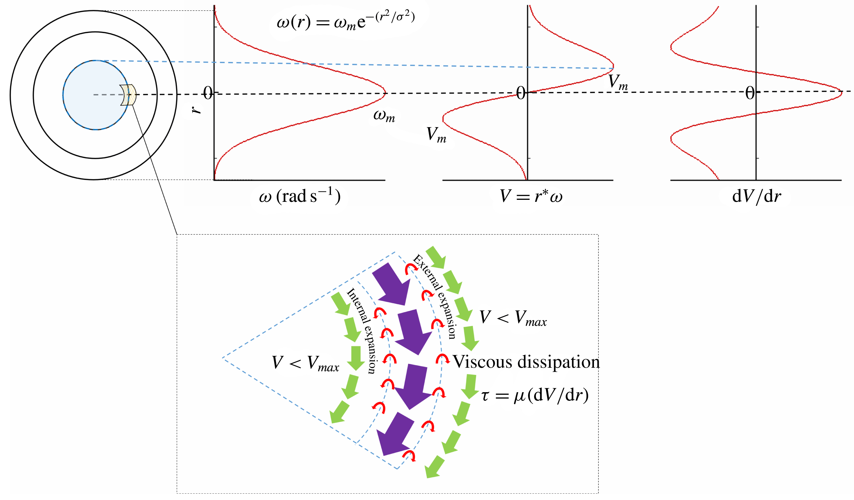
Consider a fully developed vortex at any particular time instant defined by (2.7). The vorticity and velocity fields for such a vortex are shown in figure 2. Vorticity diffusion in any Newtonian fluid is governed by viscous shear forces given by (2.8)
 $$\begin{eqnarray}\displaystyle & \displaystyle \unicode[STIX]{x1D714}_{t}(r)=\unicode[STIX]{x1D714}_{m,t}\text{e}^{-(r/\unicode[STIX]{x1D70E}_{t})^{2}} & \displaystyle\end{eqnarray}$$
 $$\begin{eqnarray}\displaystyle & \displaystyle \unicode[STIX]{x1D70F}_{t}(r)=\unicode[STIX]{x1D707}\left(\frac{\unicode[STIX]{x2202}V}{\unicode[STIX]{x2202}r}\right). & \displaystyle\end{eqnarray}$$
Please note that the angular momentum (
 $\unicode[STIX]{x1D6FA}$
) is equal to half of the vorticity. However, this numerical factor is neglected throughout this paper. Thus, for a fluid region defined as a disk of radius
 $r$
, as in figure 2, viscous stress at any time instant
 $t$
due to external shear can be calculated as
 $$\begin{eqnarray}\displaystyle & \displaystyle \unicode[STIX]{x1D70F}_{t}(r)=\unicode[STIX]{x1D707}\left(\frac{\unicode[STIX]{x2202}r\unicode[STIX]{x1D714}}{\unicode[STIX]{x2202}r}\right)=\unicode[STIX]{x1D707}\left[r\frac{\unicode[STIX]{x2202}\unicode[STIX]{x1D714}}{\unicode[STIX]{x2202}r}+\unicode[STIX]{x1D714}\right] & \displaystyle\end{eqnarray}$$
 $$\begin{eqnarray}\displaystyle & \displaystyle \unicode[STIX]{x1D70F}_{t}(r)=-\unicode[STIX]{x1D707}\left[\unicode[STIX]{x1D714}_{m,t}\text{e}^{-(r/\unicode[STIX]{x1D70E}_{t})^{2}}\left(1-\frac{2r^{2}}{\unicode[STIX]{x1D70E}_{t}^{2}}\right)\right], & \displaystyle\end{eqnarray}$$
where
 $\unicode[STIX]{x1D707}$
is the dynamic viscosity. For a stable Gaussian vorticity profile (2.7), the velocity variation is shown in figure 2. It is evident that the maximum fluid velocity occurs at a distance
 $\unicode[STIX]{x1D70E}/\sqrt{2}$
from the vortex centre. This results in complex shear interactions resulting in vorticity diffusion, internal as well as external to the locus of maximum velocity. Some prior studies regarding the evolution of Gaussian vortex rings have accounted for external as well as internal expansion of the core structure (Fraenkel Reference Fraenkel1972; Fukumoto & Moffatt Reference Fukumoto and Moffatt2000). However, numerical and experimental studies clearly show a decreasing trend in peak vorticity values and a corresponding increase in the length scale of the vorticity distribution throughout its propagation period. Previous studies also validate the claim that a fully developed vortex ring is characterized by a vorticity distribution which can be best approximated by a Gaussian profile (Saffman Reference Saffman1978; Weigand & Gharib Reference Weigand and Gharib1997). Thus, using known parameters, we propose a simpler vortex evolution model by considering only the external expansion of the vortex core. Internal interaction of the core structure is neglected and assumed to adjust itself to satisfy the Gaussian vorticity distribution parameters.
Schematic of the vorticity distribution in the core.

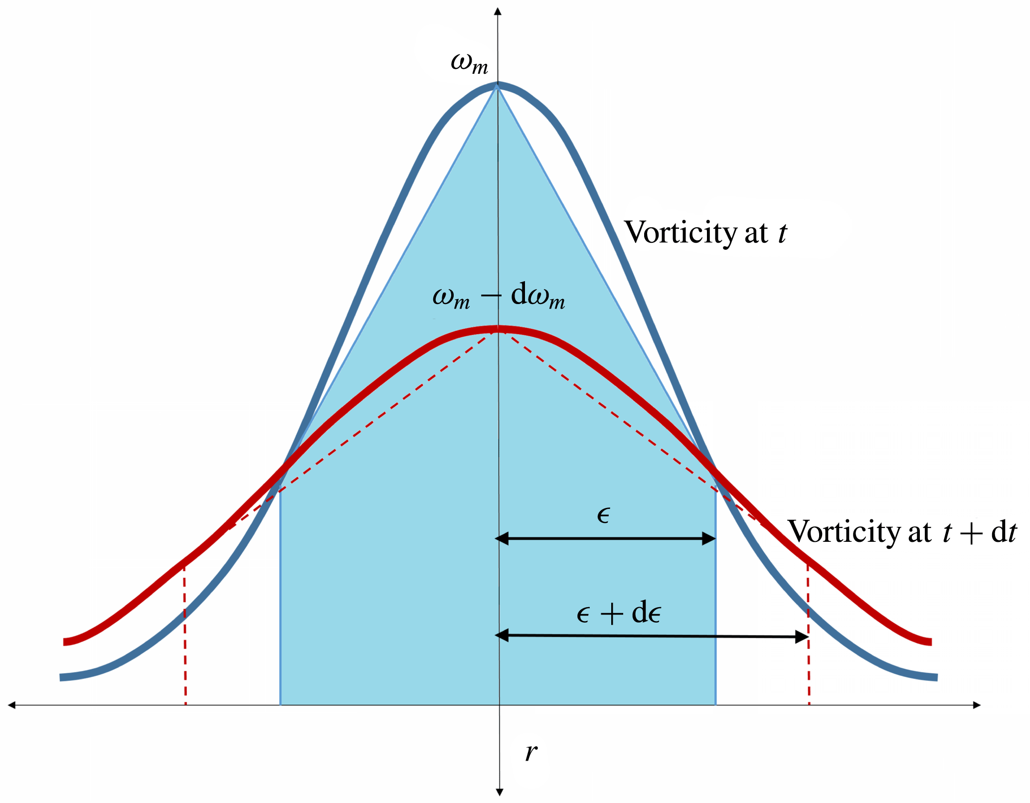
Variation of the vorticity distribution with time.
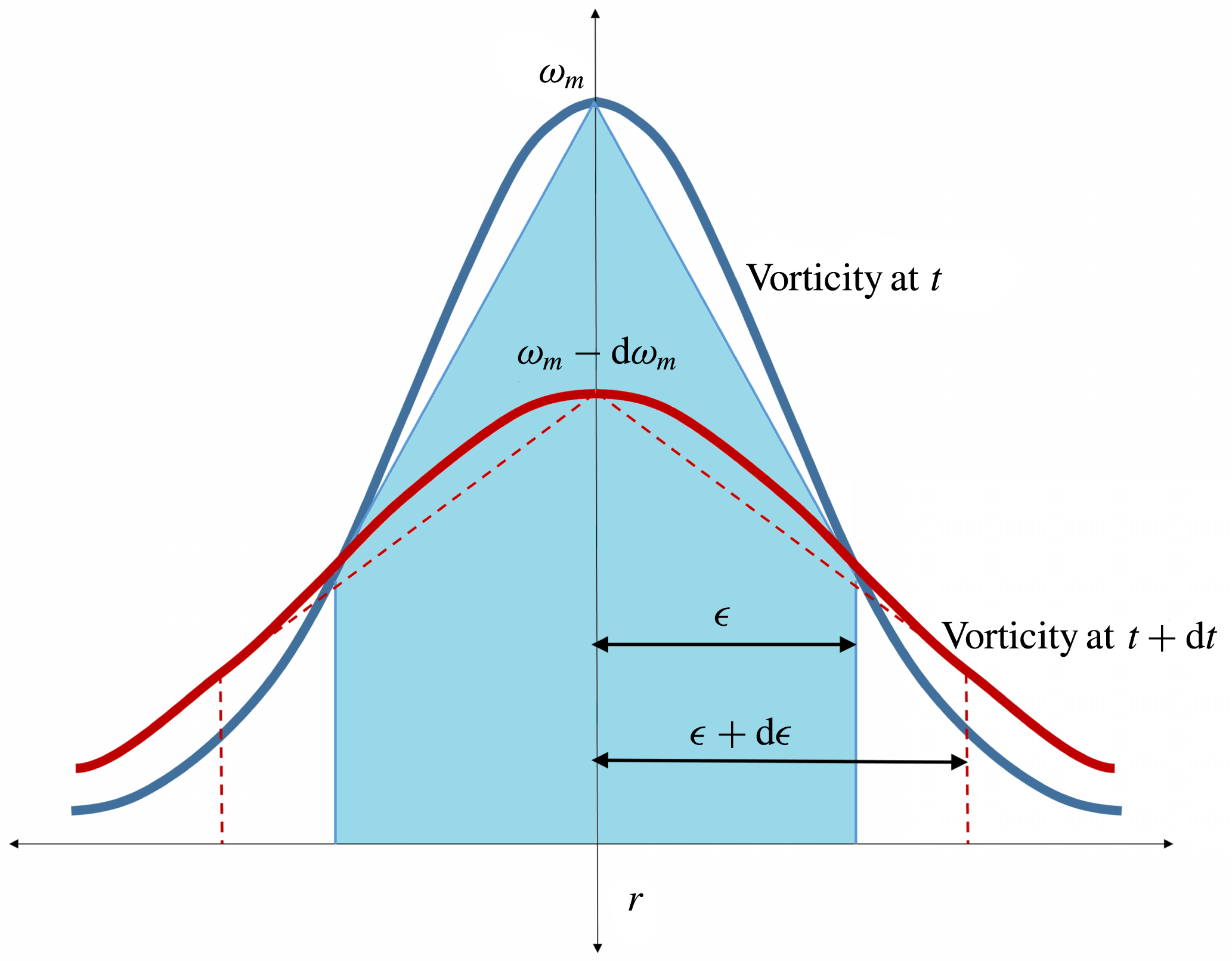
Consider the core to be a rigid disc with an approximately linear
 $\unicode[STIX]{x1D714}$
variation (2.11) and radius
 $\unicode[STIX]{x1D716}$
, as shown in figure 3. Let an arbitrary definition of the vortex core size correspond to
 $\unicode[STIX]{x1D716}=k_{1}\unicode[STIX]{x1D70E}$
and
 $\unicode[STIX]{x1D714}(\unicode[STIX]{x1D716})=k_{2}\unicode[STIX]{x1D714}_{m}$
, where
 $k_{2}=\text{e}^{-(k_{1})^{2}}$
. The vorticity distribution and angular momentum of this disc are given by
 $$\begin{eqnarray}\displaystyle & \displaystyle \unicode[STIX]{x1D714}_{t}(r)=\unicode[STIX]{x1D714}_{m,t}\left[1-\frac{1-k_{2}}{k_{1}}\frac{r}{\unicode[STIX]{x1D70E}_{t}}\right] & \displaystyle\end{eqnarray}$$
 $$\begin{eqnarray}\displaystyle & \displaystyle L=\int \text{d}I\,\unicode[STIX]{x1D714}_{t}(r)=\int _{0}^{\unicode[STIX]{x1D716}}\unicode[STIX]{x1D70C}(2\unicode[STIX]{x03C0}r\,\text{d}r\,\text{d}z)(r^{2})\unicode[STIX]{x1D714}_{m,t}\left[1-\frac{1-k_{2}}{k_{1}}\frac{r}{\unicode[STIX]{x1D70E}_{t}}\right]. & \displaystyle\end{eqnarray}$$
This above vortex disc can be defined by an average vorticity given by
 $$\begin{eqnarray}I\unicode[STIX]{x1D714}_{avg,t}=\left(\frac{\unicode[STIX]{x1D70C}\unicode[STIX]{x03C0}\unicode[STIX]{x1D716}^{4}\,\text{d}z}{2}\right)\unicode[STIX]{x1D714}_{avg,t}=L,\end{eqnarray}$$
which yields
 $$\begin{eqnarray}\unicode[STIX]{x1D714}_{avg,t}=\unicode[STIX]{x1D714}_{m,t}\left[1-\frac{4(1-k_{2})}{5}\right].\end{eqnarray}$$
Neglecting any internal fluid interactions, the net torque on the vortex core is given by (2.15). This torque will slow down the vortex core and can be assumed to alter the average vorticity, given by (2.18).
 $$\begin{eqnarray}\displaystyle & \displaystyle T(\unicode[STIX]{x1D716})=-\unicode[STIX]{x1D707}\left|\unicode[STIX]{x1D714}_{m,t}\text{e}^{-(\unicode[STIX]{x1D716}/\unicode[STIX]{x1D70E}_{t})^{2}}\left(1-\frac{2\unicode[STIX]{x1D716}^{2}}{\unicode[STIX]{x1D70E}_{t}^{2}}\right)\right|(2\unicode[STIX]{x03C0}\unicode[STIX]{x1D716})\unicode[STIX]{x1D716}\,\text{d}z & \displaystyle\end{eqnarray}$$
 $$\begin{eqnarray}\displaystyle & \displaystyle \unicode[STIX]{x1D70C}\left(\frac{\unicode[STIX]{x03C0}}{2}\unicode[STIX]{x1D716}^{4}\,\text{d}z\right)\unicode[STIX]{x1D6FC}_{avg,t}=-\unicode[STIX]{x1D707}\left|\unicode[STIX]{x1D714}_{m,t}\text{e}^{-(\unicode[STIX]{x1D716}/\unicode[STIX]{x1D70E}_{t})^{2}}\left(1-\frac{2\unicode[STIX]{x1D716}^{2}}{\unicode[STIX]{x1D70E}_{t}^{2}}\right)\right|(2\unicode[STIX]{x03C0}\unicode[STIX]{x1D716})\unicode[STIX]{x1D716}\,\text{d}z. & \displaystyle\end{eqnarray}$$
Substituting the values of
 $\unicode[STIX]{x1D716}=k_{1}\unicode[STIX]{x1D70E}$
and (2.14), where
 $k_{2}=\text{e}^{-(k_{1})^{2}}$
, we get
 $$\begin{eqnarray}\unicode[STIX]{x1D6FC}_{avg,t}=\frac{\unicode[STIX]{x2202}\unicode[STIX]{x1D714}_{avg,t}}{\unicode[STIX]{x2202}t}=-4\left|\frac{5(1-2k_{1}^{2})\text{e}^{-k_{1}^{2}}}{k_{1}^{2}(5-4(1-\text{e}^{-k_{1}^{2}}))}\right|\left(\frac{\unicode[STIX]{x1D708}\unicode[STIX]{x1D714}_{avg,t}}{\unicode[STIX]{x1D70E}_{t}^{2}}\right),\end{eqnarray}$$
which can be written as
 $$\begin{eqnarray}\frac{\unicode[STIX]{x2202}\unicode[STIX]{x1D714}_{avg,t}}{\unicode[STIX]{x2202}t}=-4\unicode[STIX]{x1D719}\left(\frac{\unicode[STIX]{x1D708}\unicode[STIX]{x1D714}_{avg,t}}{\unicode[STIX]{x1D70E}_{t}^{2}}\right),\end{eqnarray}$$
where
 $$\begin{eqnarray}\unicode[STIX]{x1D719}=\left|\frac{5(1-2k_{1}^{2})\text{e}^{-k_{1}^{2}}}{k_{1}^{2}(5-4(1-\text{e}^{-k_{1}^{2}}))}\right|.\end{eqnarray}$$
Here, the value of
 $\unicode[STIX]{x1D719}$
is satisfied by two values of
 $k_{1}$
, each on either side of
 $1/\sqrt{2}$
. However, the value of
 $k_{1}$
greater than 0.707 should be accepted. This is because such
 $k_{1}$
values lead to the appropriate sign of velocity gradients pointing away from the vortex core, signifying external dissipation. In contrast,
 $k_{1}$
less than 0.707 signifies internal viscous dissipation, which has been neglected in this derivation.
Thus, at any instant, the rate of decay of peak vorticity is directly proportional to the kinematic viscosity
 $\unicode[STIX]{x1D708}$
and
 $\unicode[STIX]{x1D714}_{m}$
, and inversely to the variance of the vorticity field. This can be easily understood intuitively. Kinematic viscosity quantifies friction between the fluid layers. Thus, higher friction will lead to greater retardation. Similarly, keeping
 $\unicode[STIX]{x1D708}$
and
 $\unicode[STIX]{x1D714}_{m}$
constant, concentrated cores will experience greater dissipation due to higher velocity gradients and vice versa. At this point, we may be tempted to perform integration to obtain the final expression of peak vorticity
 $\unicode[STIX]{x1D714}_{m}(t)$
. However, the standard deviation
 $\unicode[STIX]{x1D70E}$
is also a time-varying parameter. Hence the expression (2.18) cannot be solved further without understanding the time evolution of
 $\unicode[STIX]{x1D70E}$
.
In order to understand the variation in standard deviation
 $\unicode[STIX]{x1D70E}$
, we consider the interaction between the core disk and adjacent fluid layer. As a result of the interaction, after time
 $\text{d}t$
,
 $\unicode[STIX]{x1D714}_{avg}$
decreases by
 $\text{d}\unicode[STIX]{x1D714}_{avg}$
while the core size increases by
 $\text{d}\unicode[STIX]{x1D716}$
. Thus, the new core will have a radius of
 $(\unicode[STIX]{x1D716}+\text{d}\unicode[STIX]{x1D716})$
and a vorticity of
 $(\unicode[STIX]{x1D714}_{avg}-\text{d}\unicode[STIX]{x1D714}_{avg})$
. Using the principle of conservation of angular momentum and neglecting higher-order terms, we get
 $$\begin{eqnarray}\displaystyle & \displaystyle I_{ini}\unicode[STIX]{x1D714}_{ini}=I_{fi}\unicode[STIX]{x1D714}_{fi} & \displaystyle\end{eqnarray}$$
 $$\begin{eqnarray}\displaystyle & \displaystyle \unicode[STIX]{x1D70C}\left(\frac{\unicode[STIX]{x03C0}}{2}\right)\unicode[STIX]{x1D716}^{4}\unicode[STIX]{x1D714}_{avg,t}=\unicode[STIX]{x1D70C}\left(\frac{\unicode[STIX]{x03C0}}{2}\right)(\unicode[STIX]{x1D716}+\text{d}\unicode[STIX]{x1D716})^{4}(\unicode[STIX]{x1D714}_{avg,t}-\text{d}\unicode[STIX]{x1D714}_{avg,t}) & \displaystyle\end{eqnarray}$$
 $$\begin{eqnarray}\displaystyle & \displaystyle k_{1}^{4}\unicode[STIX]{x1D716}^{4}\unicode[STIX]{x1D714}_{avg,t}=k_{1}^{4}(\unicode[STIX]{x1D70E}_{t}^{4}+4\unicode[STIX]{x1D70E}_{t}^{2}\,\text{d}\unicode[STIX]{x1D70E}_{t})\left(\unicode[STIX]{x1D714}_{avg,t}-\unicode[STIX]{x1D714}_{avg,t}4\unicode[STIX]{x1D719}\left(\frac{\unicode[STIX]{x1D708}}{\unicode[STIX]{x1D70E}_{t}^{2}}\right)\,\text{d}t\right) & \displaystyle\end{eqnarray}$$
 $$\begin{eqnarray}\displaystyle & \displaystyle \frac{\text{d}\unicode[STIX]{x1D70E}_{t}}{\text{d}t}=\unicode[STIX]{x1D719}\left(\frac{\unicode[STIX]{x1D708}}{\unicode[STIX]{x1D70E}_{t}}\right) & \displaystyle\end{eqnarray}$$
 $$\begin{eqnarray}\displaystyle & \displaystyle \unicode[STIX]{x1D70E}_{t}=\sqrt{\unicode[STIX]{x1D70E}_{0}^{2}+2\unicode[STIX]{x1D719}\unicode[STIX]{x1D708}t}. & \displaystyle\end{eqnarray}$$
Thus, the variation in the standard deviation of vorticity is given by (2.24), where
 $\unicode[STIX]{x1D70E}_{0}$
is the standard deviation at a user-defined initial time. It is worth noting that the rate of change of standard deviation is independent of the peak vorticity
 $\unicode[STIX]{x1D714}_{m}$
, and depends only on the kinematic viscosity and instantaneous standard deviation.
In the above derivation, the conservation principle is applied to the entire system, comprising of the internal disk plus the adjoining fluid region. In contrast, equations (2.15) and (2.18) refer to the viscous effects on the internal fluid disk only. This conservation principle is applied considering the validity of Newton’s law that the total angular momentum of a system remains unaltered under the action of torques internal to the system. As the viscous torque retards the internal disk, it has an equal and opposite influence on the surrounding fluid layer. The adjoining layer thus gains momentum, keeping the total momentum of the configuration constant.
Using the above result, (2.18) can be modified and solved for peak vorticity variation (2.26),
 $$\begin{eqnarray}\frac{\unicode[STIX]{x2202}\unicode[STIX]{x1D714}_{avg,t}}{\unicode[STIX]{x2202}t}=-4\unicode[STIX]{x1D719}\frac{\unicode[STIX]{x1D708}\unicode[STIX]{x1D714}_{avg,t}}{(\unicode[STIX]{x1D70E}_{0}^{2}+2\unicode[STIX]{x1D719}\unicode[STIX]{x1D708}t)}\end{eqnarray}$$
 $$\begin{eqnarray}\unicode[STIX]{x1D714}_{avg,t}=\frac{\unicode[STIX]{x1D714}_{avg,0}}{\displaystyle \left[1+\frac{2\unicode[STIX]{x1D719}\unicode[STIX]{x1D708}t}{\unicode[STIX]{x1D70E}_{0}^{2}}\right]^{2}}\quad \text{i.e. }\unicode[STIX]{x1D714}_{m,t}=\frac{\unicode[STIX]{x1D714}_{m,0}}{\displaystyle \left[1+\frac{2\unicode[STIX]{x1D719}\unicode[STIX]{x1D708}t}{\unicode[STIX]{x1D70E}_{0}^{2}}\right]^{2}}.\end{eqnarray}$$
From (2.26) and (2.24) it can be seen that the maximum vorticity decreases as the square of the time whereas the standard deviation increases as the square root of time. Thus, the vorticity distribution inside the vortex can be written as
 $$\begin{eqnarray}\unicode[STIX]{x1D714}(r,t)=\frac{\unicode[STIX]{x1D6E4}_{0}}{(\unicode[STIX]{x1D70E}_{0}^{2}+2\unicode[STIX]{x1D719}\unicode[STIX]{x1D708}t)}\text{e}^{-(r/\sqrt{\unicode[STIX]{x1D70E}_{0}^{2}+2\unicode[STIX]{x1D719}\unicode[STIX]{x1D708}t})^{2}},\end{eqnarray}$$
where
 $\unicode[STIX]{x1D6E4}_{0}=\unicode[STIX]{x03C0}\unicode[STIX]{x1D714}_{m,0}\unicode[STIX]{x1D70E}_{0}^{2}$
. Using these values, we can find the circulation at any instant of time by computing the area integral of vorticity within a closed contour
 $C$
around the vortex core:
 $$\begin{eqnarray}\displaystyle & \displaystyle \unicode[STIX]{x1D6E4}\propto \int \unicode[STIX]{x1D714}\,\text{d}\unicode[STIX]{x1D713}=\unicode[STIX]{x03C0}\unicode[STIX]{x1D70E}^{2}\unicode[STIX]{x1D714}_{m} & \displaystyle\end{eqnarray}$$
 $$\begin{eqnarray}\displaystyle & \displaystyle \unicode[STIX]{x1D6E4}\propto \frac{\unicode[STIX]{x03C0}\unicode[STIX]{x1D70E}_{0}^{4}\unicode[STIX]{x1D714}_{m,0}}{(\unicode[STIX]{x1D70E}_{0}^{2}+2\unicode[STIX]{x1D719}\unicode[STIX]{x1D708}t)}=\frac{\unicode[STIX]{x1D6E4}_{0}}{\displaystyle \left(1+\frac{2\unicode[STIX]{x1D719}\unicode[STIX]{x1D708}t}{\unicode[STIX]{x1D70E}_{0}^{2}}\right)}. & \displaystyle\end{eqnarray}$$
Thus, in the case of viscous fluids, the vortex circulation decreases with time. Although fluid viscosity results in loss of circulation, it is believed that in the absence of body forces the total hydrodynamic impulse imparted to a system cannot change (Batchelor Reference Batchelor2000). Therefore, the total impulse given by (2.30), where
 $a$
is a ring radius, must be conserved:
 $$\begin{eqnarray}I\propto \unicode[STIX]{x1D6E4}a^{2}.\end{eqnarray}$$
Considering the variation in circulation given by (2.29), temporal variations in vortex spacing
 $a$
can be derived as
 $$\begin{eqnarray}a=a_{0}\sqrt{1+\frac{2\unicode[STIX]{x1D719}\unicode[STIX]{x1D708}t}{\unicode[STIX]{x1D70E}_{0}^{2}}}.\end{eqnarray}$$
For a vortex ring defined by (2.27), the propagation velocity at a point on the ring axis can be calculated using Biot–Savart’s law in polar coordinates as
 $$\begin{eqnarray}\boldsymbol{V}(x,y,z)=\frac{\unicode[STIX]{x1D6E4}}{4\unicode[STIX]{x03C0}}\int _{0}^{2\unicode[STIX]{x03C0}}\frac{r\,\mathbf{d}\unicode[STIX]{x1D73D}\times \boldsymbol{r}}{|\boldsymbol{r}|^{3}}.\end{eqnarray}$$
Using Saffman’s equation for viscous fluids (1.2) and applying it to our vorticity profile, we calculate the vortex propagation velocity at the leading order, given by
 $$\begin{eqnarray}V=\frac{\unicode[STIX]{x1D6E4}}{4\unicode[STIX]{x03C0}a}\left[\ln \left(\frac{8a}{\unicode[STIX]{x1D70E}}\right)-0.558\right]=\frac{\unicode[STIX]{x1D6E4}_{0}}{4\unicode[STIX]{x03C0}a_{0}\displaystyle \left(1+\frac{2\unicode[STIX]{x1D719}\unicode[STIX]{x1D708}t}{\unicode[STIX]{x1D70E}_{0}^{2}}\right)^{3/2}}\left\{\ln \left(\frac{8a_{0}}{\unicode[STIX]{x1D70E}_{0}}\right)-0.558\right\}.\end{eqnarray}$$
The above equation clearly shows that, for larger times
 $t$
, circulation of the vortex reduces hyperbolically while the corresponding propagation velocity is proportional to
 $t^{-3/2}$
. This decreasing velocity trend was first observed by Reynolds (Reference Reynolds1876). He attributed this to entrainment effects resulting in growing vortex size.
The above-derived equations can be written in non-dimensional form as
 $$\begin{eqnarray}t^{\ast }=\frac{2\unicode[STIX]{x1D719}\unicode[STIX]{x1D708}t}{\unicode[STIX]{x1D70E}_{0}^{2}},\quad \unicode[STIX]{x1D714}^{\ast }=\frac{\unicode[STIX]{x1D714}_{m,t}}{\unicode[STIX]{x1D714}_{m,0}}=\frac{1}{(1+t^{\ast })^{2}},\quad \unicode[STIX]{x1D70E}^{\ast }=\frac{\unicode[STIX]{x1D70E}_{t}}{\unicode[STIX]{x1D70E}_{0}}=\sqrt{1+t^{\ast }}\end{eqnarray}$$
 $$\begin{eqnarray}a^{\ast }=\frac{a_{t}}{a_{0}}=\sqrt{1+t^{\ast }},\quad \unicode[STIX]{x1D6E4}^{\ast }=\frac{\unicode[STIX]{x1D6E4}_{t}}{\unicode[STIX]{x1D6E4}_{0}}=\frac{1}{(1+t^{\ast })},\quad V^{\ast }=\frac{V_{t}}{V_{0}}=\frac{1}{(1+t^{\ast })^{3/2}}\end{eqnarray}$$
These results are in good agreement with the equations proposed by Saffman (Reference Saffman1970) and Reynolds (Reference Reynolds1876). However, these are somewhat different from those obtained by Maxworthy (Reference Maxworthy1972). He attributed the loss of vorticity to the wake. Our equations are derived by considering the macroscopic aspects of vortex evolution and no reasoning is yet provided for the mechanism responsible for loss of circulation. A detailed reasoning towards circulation reduction will be provided in § 5. Moreover, these equations are derived considering the same fundamental assumptions as used by Maxworthy: (i) the vortex distribution is Gaussian and symmetric about the core centre; (ii) any changes in vorticity due to internal or external viscous effects are reflected instantaneously by an overall change in the vorticity distribution, and (iii) the total impulse of the vortex ring remains constant. These assumptions have been scrutinized in greater detail in § 5.
Though the results do not seem to bring any major advancement over the already available theory of Saffman, we would like to emphasize the importance of this model on a couple of fronts. Firstly, here we have approached the finite thickness vorticity diffusion problem using a completely new dimension which has enabled us to formulate a simple pseudo self-similar solution. This is a major advancement considering the complex non-self-similar mathematical solutions of such cases (§ 2.1). Secondly, while deriving long-term limits, for thick core vortex equations, Saffman (Reference Saffman1970) explicitly solved for Hill’s spherical vortex with a core size equal to half of the vortex spacing. Thus, his theory does not completely comply to cases with slenderness ratio less than unity. Saffman (Reference Saffman1970) also reported this fact. Also, his model does not help us in determining the variation of core size and peak vorticity values, which are important vortex parameters. These are critically addressed in the current model. Although the current effort does not negate or disprove any of the previous results, the elegant mathematical formulation of the problem in § 2 helps us to better understand its validity and scope. It also helps us to derive a transitional theory in § 5.
We also realize that the current model is not a controlled approximation of the vorticity equation and has been solved using an unconventional approach. Thus, some important aspects must be remembered. Firstly, the solution has been obtained for an isodensity, isoviscosity fluid. Thus, the solution is applicable only to non-buoyant cases. Further, this approach is derived based on a Gaussian axisymmetric vorticity profile, and any deviation from these assumptions will affect the accuracy of the model. Therefore, the current model may not work effectively for extremely thin rings or point vortices, where the vorticity distribution may be highly localized. Also, it may perform unsatisfactorily for very thick cores due to the significant skewness in their Gaussian profiles. Lastly, the effects of any vortex instabilities have not been considered.
There have been many exhaustive studies on vortex evolution where the effects of convective velocity on vortex geometry have also been considered (Fraenkel Reference Fraenkel1972). In practical cases, the local flow induced by vortex rings consists of not only circular vorticity fields, but also the self-induced straining field resulting from translational motion. This straining field manifests itself at second order and deforms the core into an ellipse elongated in the propagating direction (Fraenkel Reference Fraenkel1972; Dyson Reference Dyson1893). The relative effect of the straining field is dependent on the fluid properties, with viscosity playing an important part in selecting the realized vorticity profile. Quadrupole components operate only at
 $O(\unicode[STIX]{x1D708}/\unicode[STIX]{x1D6E4})$
, leading to an elliptic vorticity distribution where the major axis of the ellipse is inclined at
 $45^{\circ }$
to the principal axis of the external strain (Fukumoto & Moffatt Reference Fukumoto and Moffatt2000; Fukumoto & Kaplanski Reference Fukumoto and Kaplanski2008).
3 Experimental details
3.1 Experimental set-up
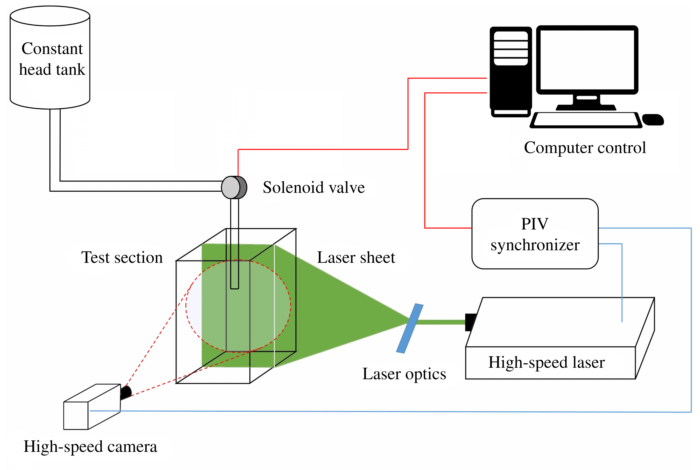
Experiments have been performed to provide supportive evidence for the claims related to the current theoretical study. A schematic of the experimental set-up is shown in figure 4. It consists of a cubic test section of dimensions
 $140~\text{mm}\times 140~\text{mm}\times 500~\text{mm}$
, with an opening at the top and transparent glass walls on all four sides. Optical accessibility is maintained to facilitate sophisticated imaging by techniques such as shadowgraphy, particle image velocimetry (PIV) and laser induced fluorescence (LIF).
Experimental set-up with imaging modalities.
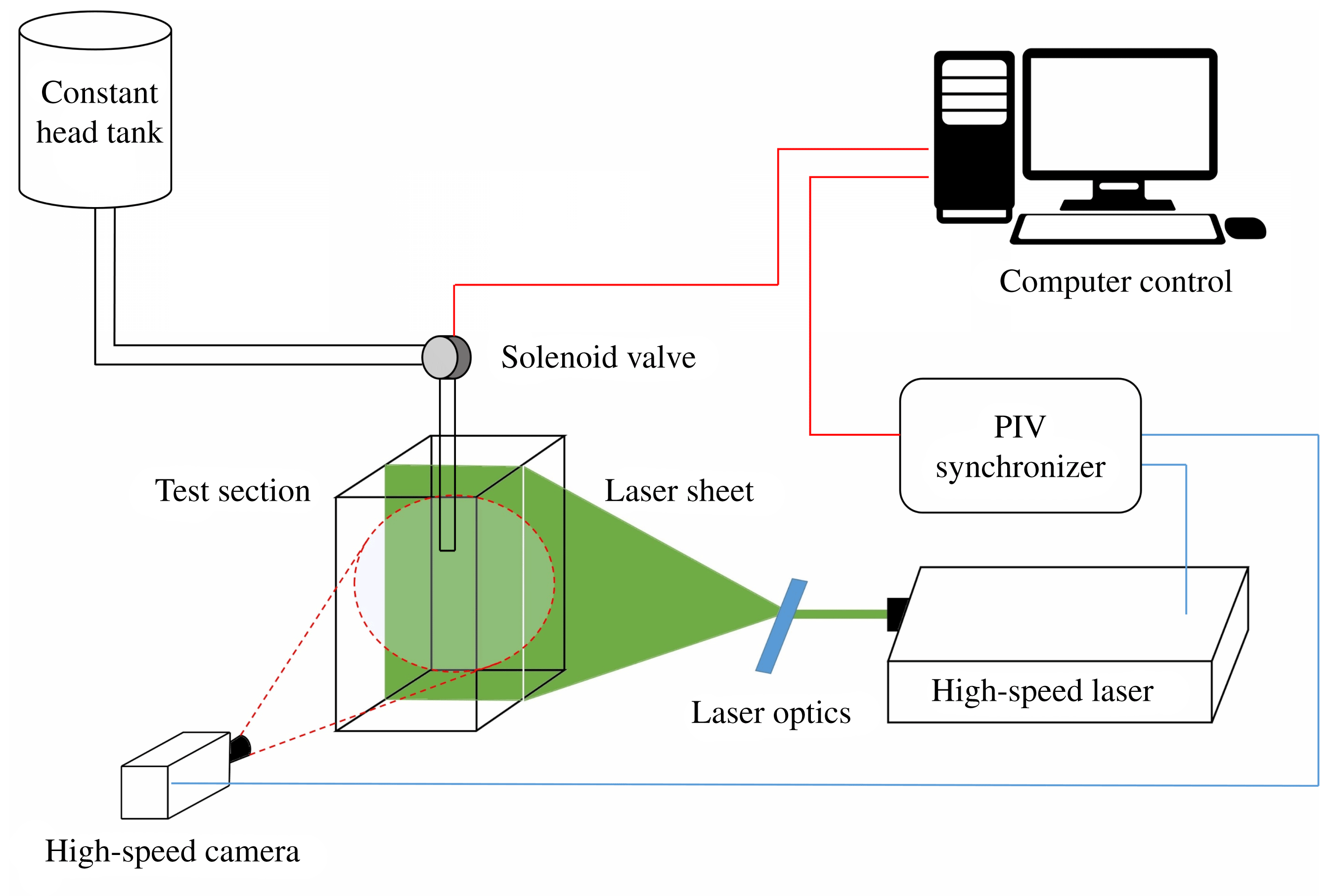
The vortex ring is introduced into the fluid domain from the top through a centrally located nozzle of diameter 15 mm. The fluid inlet was adjusted with the help of a solenoid valve connected to a LabVIEW-assisted computerized system. This ensured accurate control and proper synchronization of the experimental set-up. Vortex parameters are controlled by changing the valve opening time
 $t_{0}$
. The maximum valve opening time is limited by the formation number (
 $L/D_{n}$
) (Gharib et al.
Reference Gharib, Rambod and Shariff1998).
3.2 Imaging techniques
Flow behaviour was visualized using high-speed LIF and PIV. The LIF technique was used here to capture the spatial properties of vortex structures. Here a CNI Optoelectronics continuous laser of 3 watt power with an emission wavelength of 523 nm was used to make a light sheet of 1 mm thickness. The injected fluid was mixed with Rhodamine B dye for visualization. A high-resolution camera (Nikon D7200) was used to capture images at a resolution of
 $6000\times 4000$
pixels. Here the vortex formation, evolution and entrainment effects were clearly visible. LIF images have a higher resolution than PIV images, and thus LIF is the most sought after technique for studying vortex structures (Johari & Fang Reference Johari and Fang1997; Bond & Johari Reference Bond and Johari2010). Although LIF offers a higher resolution and crisp images, often the diffusion coefficient of the dye is less than the diffusion of vorticity (Maxworthy Reference Maxworthy1972). Therefore, LIF images may not provide an accurate interpretation of the vortex size and its spatiotemporal growth.
Dynamical properties of the vortex ring, such as velocity, vorticity distribution and circulation, were captured using a high-speed LaVision PIV system. Hollow borosilicate glass spheres of density
 $1.1~\text{g}~\text{cm}^{-3}$
and mean diameter
 $9{-}13~\unicode[STIX]{x03BC}\text{m}$
were used as seeding particles. A high-speed dual-pulsed Nd:YLF Photonics laser was used to generate a thin laser sheet of thickness 1 mm using a divergent sheet-making optics and telescopic lens arrangement. The LaVision Davis 8.2 software was used to process 2D displacement vectors at the centre plane. Imaging was performed using a Photron model SA-5 camera positioned normal to the image plane (figure 4) at a distance of 1 m. Images were captured at 500 Hz with a spatial resolution of
 $1024\times 1024$
pixels. The time interval between two successive lasers pulses was kept at 600 ns. This interval was arrived at in accordance with the optimal shift of particles within two frames (Keane & Adrian Reference Keane and Adrian1990). The experimental configuration enabled us to capture a field of view of
 $140~\text{mm}\times 140~\text{mm}$
.
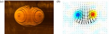
Experimental picture: (a) LIF of a fully developed vortex ring and (b) the corresponding PIV contour.

Postprocessing was performed using an interrogation window size of
 $12\times 12$
with 50 % overlap. The seeding density was adjusted such that the maximum number of particles per interrogation window was limited to 10 (Raffel et al.
Reference Raffel, Willert, Wereley and Kompenhans2013). This processing condition resulted in a field measurement of
 $171\times 171$
velocity vectors with an optimized spatial resolution of
 $0.789\times 0.789~\text{mm}$
. Such a high resolution was necessary to accurately capture the vorticity distribution inside the core.
3.3 Methodologies
Data files generated from PIV were imported into MATLAB for data processing. Azimuthal vorticity (
 $\unicode[STIX]{x1D714}$
) values were calculated using the central-difference scheme as below:
 $$\begin{eqnarray}\unicode[STIX]{x1D714}_{x,y}=\frac{V_{x+1}-V_{x-1}}{2\unicode[STIX]{x0394}y}-\frac{U_{y+1}-U_{y-1}}{2\unicode[STIX]{x0394}y}.\end{eqnarray}$$
Vortex cores were located (
 $X1,Y1$
) and (
 $X2,Y2$
) by tracking maximum and minimum values of azimuthal vorticity (
 $\unicode[STIX]{x1D714}$
) in the entire domain. Using these values, the vortex spacing
 $2a$
at any instant was extracted by calculating the geometric distance between the core centres:
 $$\begin{eqnarray}2a=\sqrt{(X1-X2)^{2}+(Y1-Y2)^{2}}.\end{eqnarray}$$
For the majority of the calculations, the vertical position of the vortex cores of both clockwise and anticlockwise vortices coincided with each other, which guaranteed a linear vertical translation of the vortex rings. The displacement
 $L_{p}$
was then calculated by taking the absolute difference between the ‘
 $Y$
’ locations of vortex core and the location of the nozzle exit.
 $$\begin{eqnarray}L_{p}=|Y1-Y_{n}|.\end{eqnarray}$$
The circulation was obtained by performing area integration of the vorticity fields within a fixed closed circular contour of
 $\text{radius}=5~\text{mm}$
centred at the location of
 $\unicode[STIX]{x1D714}_{m}$
. The vorticity distribution along a horizontal line passing through the vortex core was used for calculating the interpolated value of the standard deviation for the Gaussian profile. This value was calculated in the direction of the ring axis. These methodologies have been kept consistent throughout our study.
3.4 Experimental conditions
For our experimental set-up, stroke length
 $L$
can be defined as a product of outlet velocity
 $V_{0}$
and valve opening time
 $t_{0}$
(
 $L=V_{0}t_{0}$
). Since
 $V_{0}$
is governed by the pressure head inside the tank, which remains almost constant, we change the inlet conditions for experiments by altering the value of the valve opening time
 $t_{0}$
. Using this method, we have performed studies for a wide range of inlet conditions. The approximate value of the circulation imparted was calculated from PIV data at the beginning of the evolution period. Care was taken to keep the inlet Reynolds number (
 $Re_{0}$
) and
 $L/D_{n}$
ratio within limits.
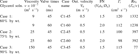
Experiments were conducted using aqueous glycerol solution at three different concentrations and different valve opening times. The density of solution remained roughly in the range
 $1.05{-}1.15~\text{g}~\text{cm}^{-3}$
while the kinematic viscosity varied from 9 to
 $180~\text{centipoise}~\text{mPa}^{-1}~\text{s}^{-1}$
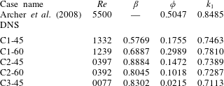
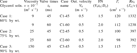
. Based on the vortex circulation, the Reynolds numbers obtained varied in the range from 50 to 1500. Further details of the operating conditions have been given in table 1. Each case was repeated three times to assure repeatability.
Experimental and operating conditions.
4 Results
4.1 Preliminary observations
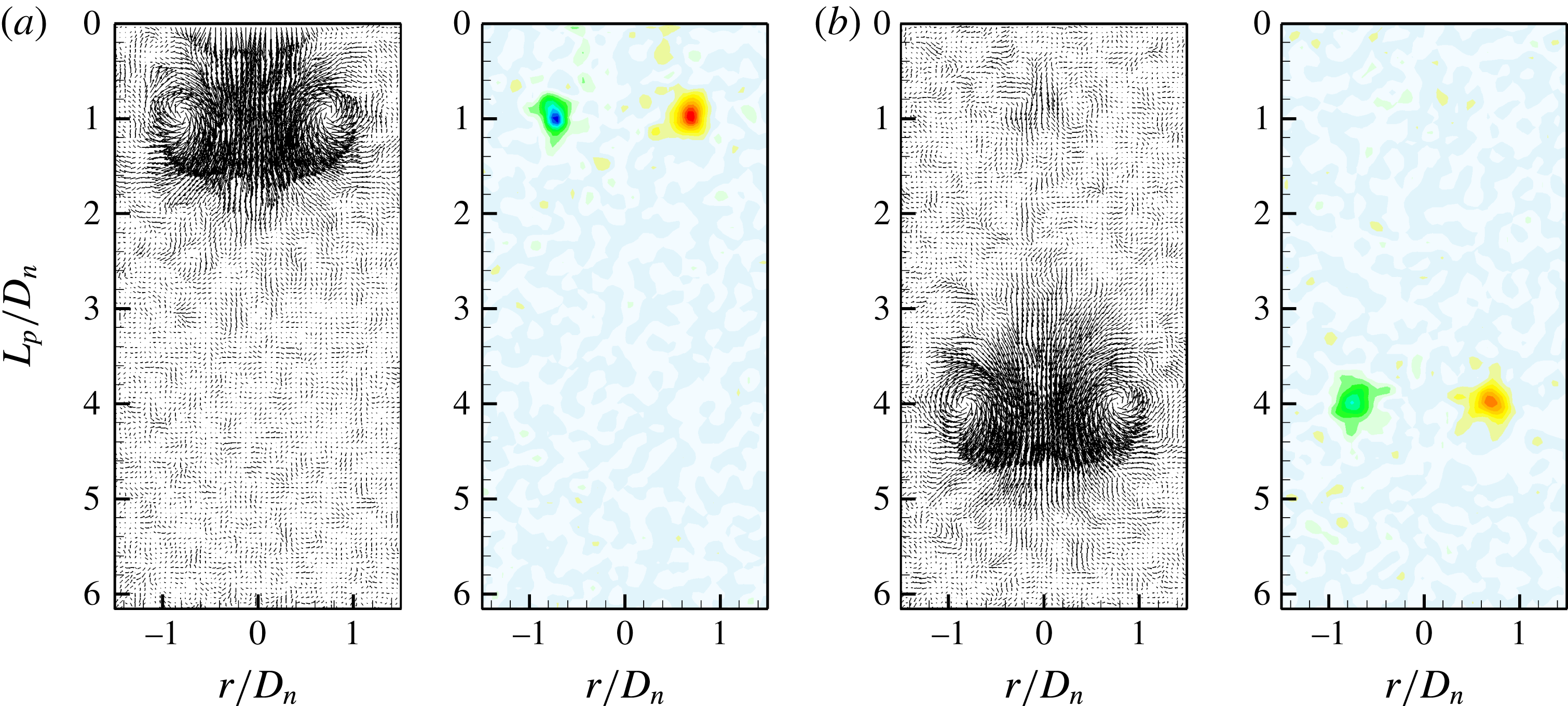
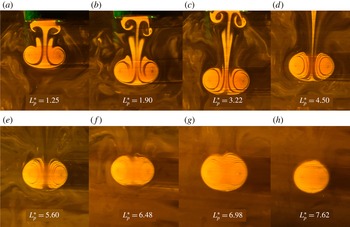
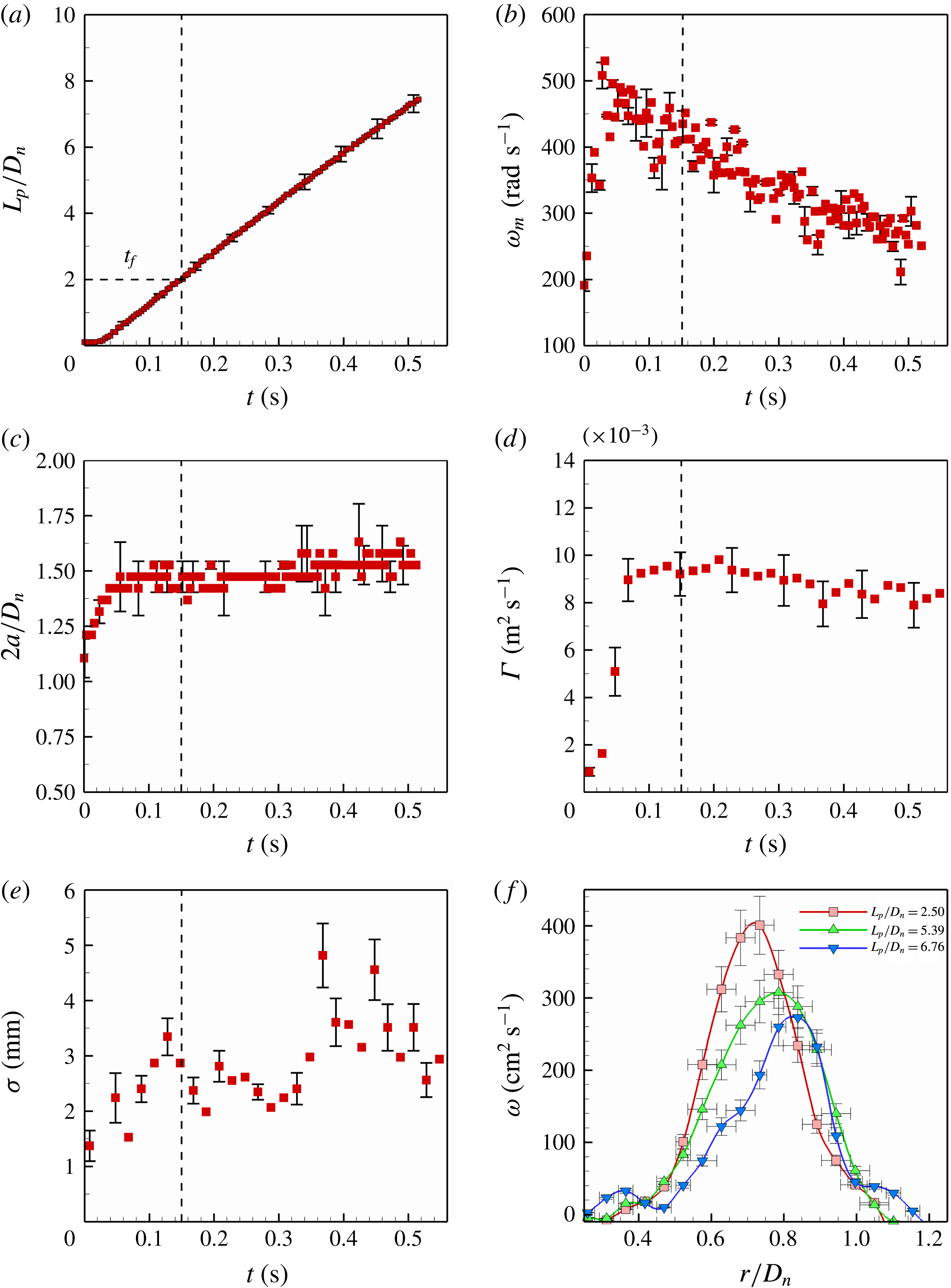
Figure 6 shows the variation in vorticity distribution over time. Initially, the injected fluid curls around the nozzle edge, leading to vortex formation, as visible in figure 7(a,b). During this period (
 $t_{f}$
), the vortex entrains surrounding fluid into the ring, leading to a considerable and sharp increase in peak vorticity (
 $\unicode[STIX]{x1D714}_{m}$
), ring size (
 $2a$
) and circulation (
 $\unicode[STIX]{x1D6E4}$
), as shown in figure 8(b–d). Figure 7(a–c) shows LIF images of the initial vortex formation period from injection to pinch off. This vortex is underdeveloped with sharp and asymmetric variations in vorticity. This transient phase ends with closing of the nozzle valve after the vortex has propagated a distance of approximately 2–3 times the nozzle diameter (figure 8
a). This termination of the development period is marked by a sudden drop in the circulation and vortex spacing, which is evident from figures 7 and 8. After this initial formation period, the vorticity gets distributed smoothly throughout the vortex core. The radial distribution of vorticity for experimental case C2-60 at different locations (
 $L_{p}/D_{n}$
) is shown in figure 8(f). These stable vorticity variations closely mimic the Gaussian distribution (Weigand & Gharib Reference Weigand and Gharib1997; Cater, Soria & Lim Reference Cater, Soria and Lim1998). Parameters such as the maximum vorticity value and standard deviation
 $\unicode[STIX]{x1D70E}$
depend on the inlet conditions and dynamics during the vortex formation phase
 $t_{f}$
.
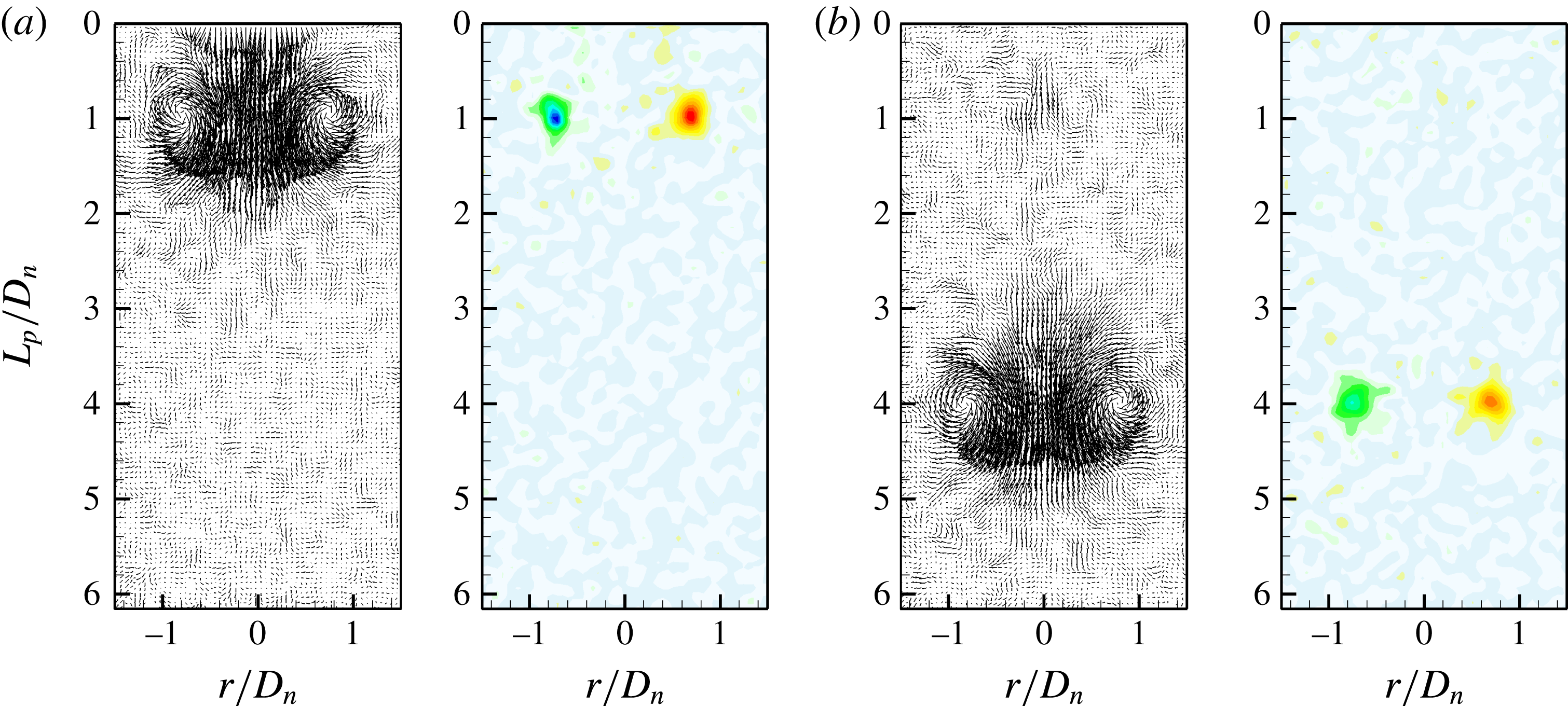
PIV vector and vorticity contour plots for C2-60 at (a)
 $L_{p}/D_{n}=1$
and (b)
 $L_{p}/D_{n}=4$
.
Flow visualization images of vortex ring at different positions during its propagation for C2-60.

Beyond
 $t_{f}$
, the vortex propagates in its self-induced field with predictable dynamics. Figure 7(d–f) show steady evolution of vortex rings. We have focused our attention on this developed regime, neglecting the initial transient effects.
Figure 8 shows the variation in vortex ring parameters with respect to time for the C2-60 case. Preliminary observations (figure 8
a) show a linear trend in vortex translation with negligible acceleration. However, considerable exponential decay can be observed for the peak vorticity values (figure 8
b). For the C2-60 case, the peak vorticity reduces by approximately 30 % in a short time span of 0.3 s. Contours shown in figure 6 offer greater insights into this phenomenon. A similar trend is seen in the variation of circulation (
 $\unicode[STIX]{x1D6E4}$
) (figure 8
d). This reduction of vorticity and circulation is attributed to viscous dissipation of the vorticity.
PIV obtained graphs of C2-60 for vortex parameters: (a)
 $L_{p}/D_{n}$
versus
 $t$
, (b)
 $\unicode[STIX]{x1D714}_{m}$
versus
 $t$
, (c)
 $2a/D_{n}$
versus
 $t$
, (d)
 $\unicode[STIX]{x1D6E4}$
versus
 $t$
, (e)
 $\unicode[STIX]{x1D70E}$
versus
 $t$
, (f)
 $\unicode[STIX]{x1D714}$
versus
 $r/D_{n}$
.
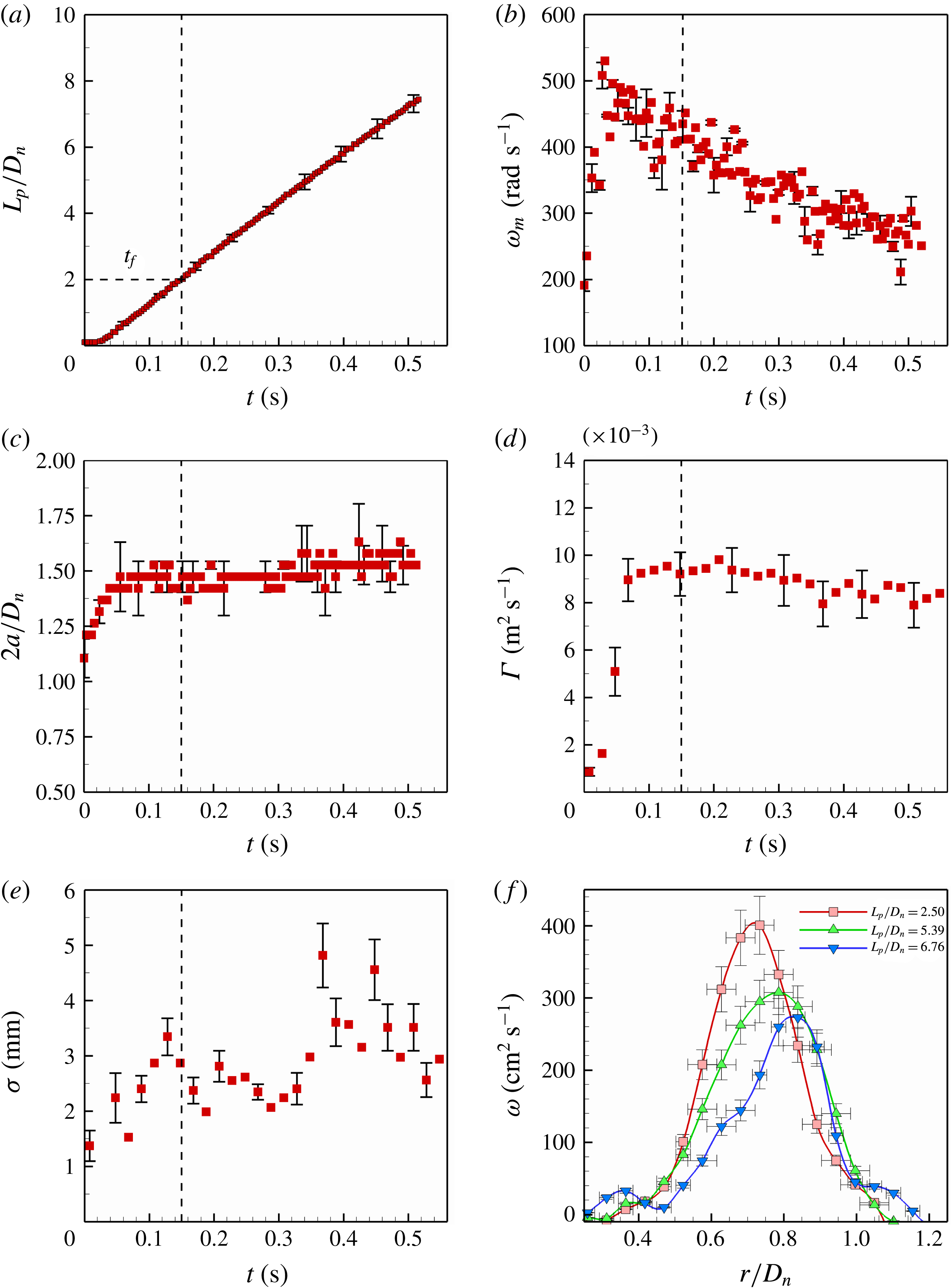
The decrease in maximum vorticity is complemented by a corresponding increase in the vorticity distribution. As the vortex propagates, it entrains the surrounding, initially irrotational fluid. This increases its bulk mass, sharing its vorticity in the process. Thus, the standard deviation
 $\unicode[STIX]{x1D70E}$
of the Gaussian distribution increases with time, as shown in figure 8(e). These variations in the vorticity distribution are considered to be largely governed by viscous effects. Therefore, for inviscid fluids, vorticity does not decay and remains concentrated in thin cores. For such cases, the circulation remains conserved. In addition to vorticity dissipation, the ring radius
 $a$
is also observed to increase. From figure 8(c), it can be seen that this increase is negligible initially. However, this rate increases as time progresses, and significant expansion effects are seen at larger times.
It is also important to note that all the variables except
 $\unicode[STIX]{x1D70E}$
show high repeatability, with errors within 10 % of the mean. High scatter is seen in the graph of
 $\unicode[STIX]{x1D70E}$
. This is due to the limited resolution of PIV, where
 $\unicode[STIX]{x1D70E}$
values are comparable with the least count of our vector resolution. Although figure 8 shows trends only for the C2-60 case, similar behaviour is observed for other test cases also. However, the quantitative aspects of these variations depend on the vortex geometry and fluid viscosity. Greater insights into these aspects are provided in § 5.
Comparison between C2-45 and C2-60: (a)
 $L_{p}/D_{n}$
versus
 $t$
, (b)
 $\unicode[STIX]{x1D714}_{m}$
versus
 $t$
, (c)
 $2a/D_{n}$
versus
 $t$
, (d)
 $\unicode[STIX]{x1D6E4}$
versus
 $t$
.
4.2 Comparison between cases
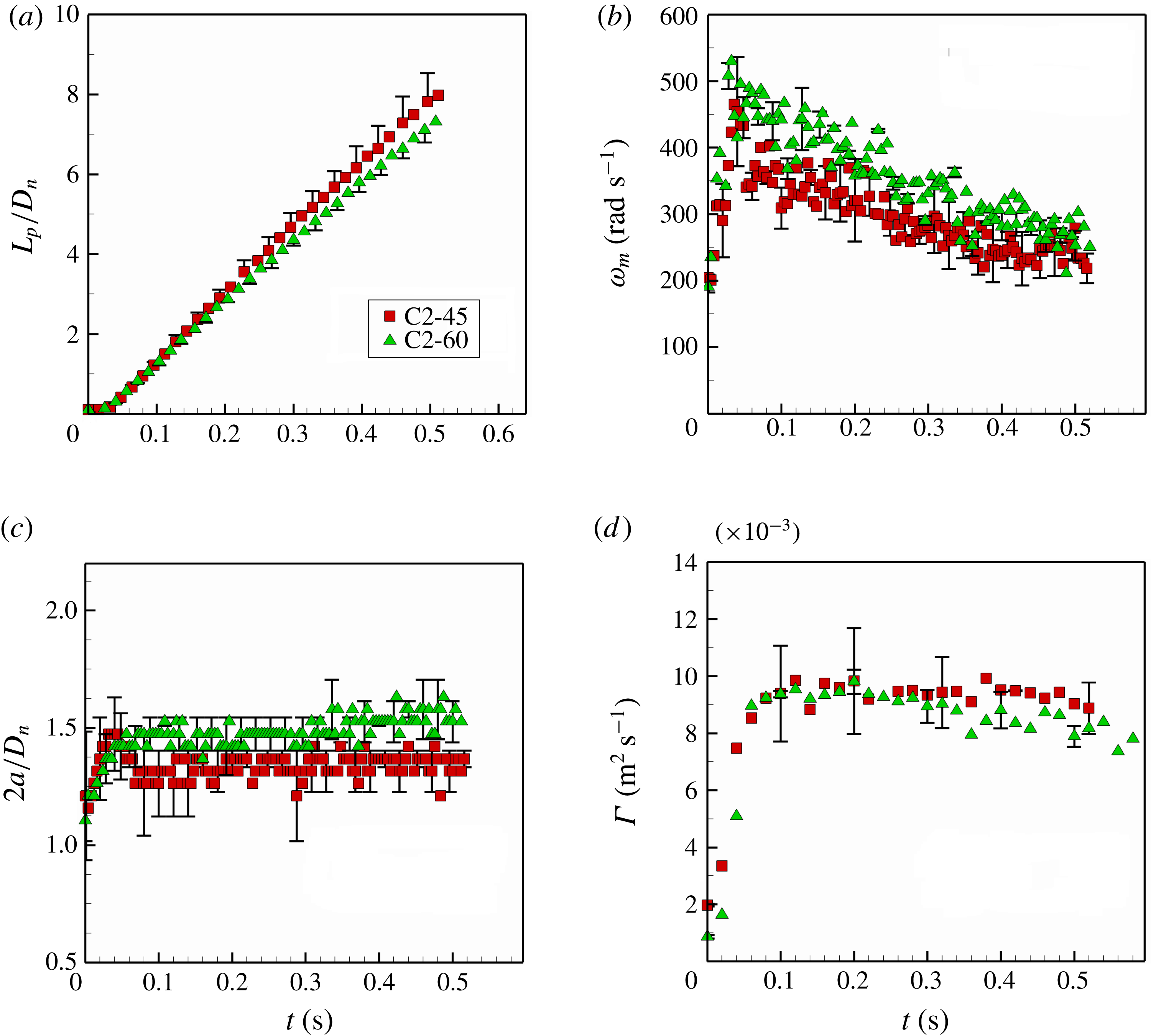
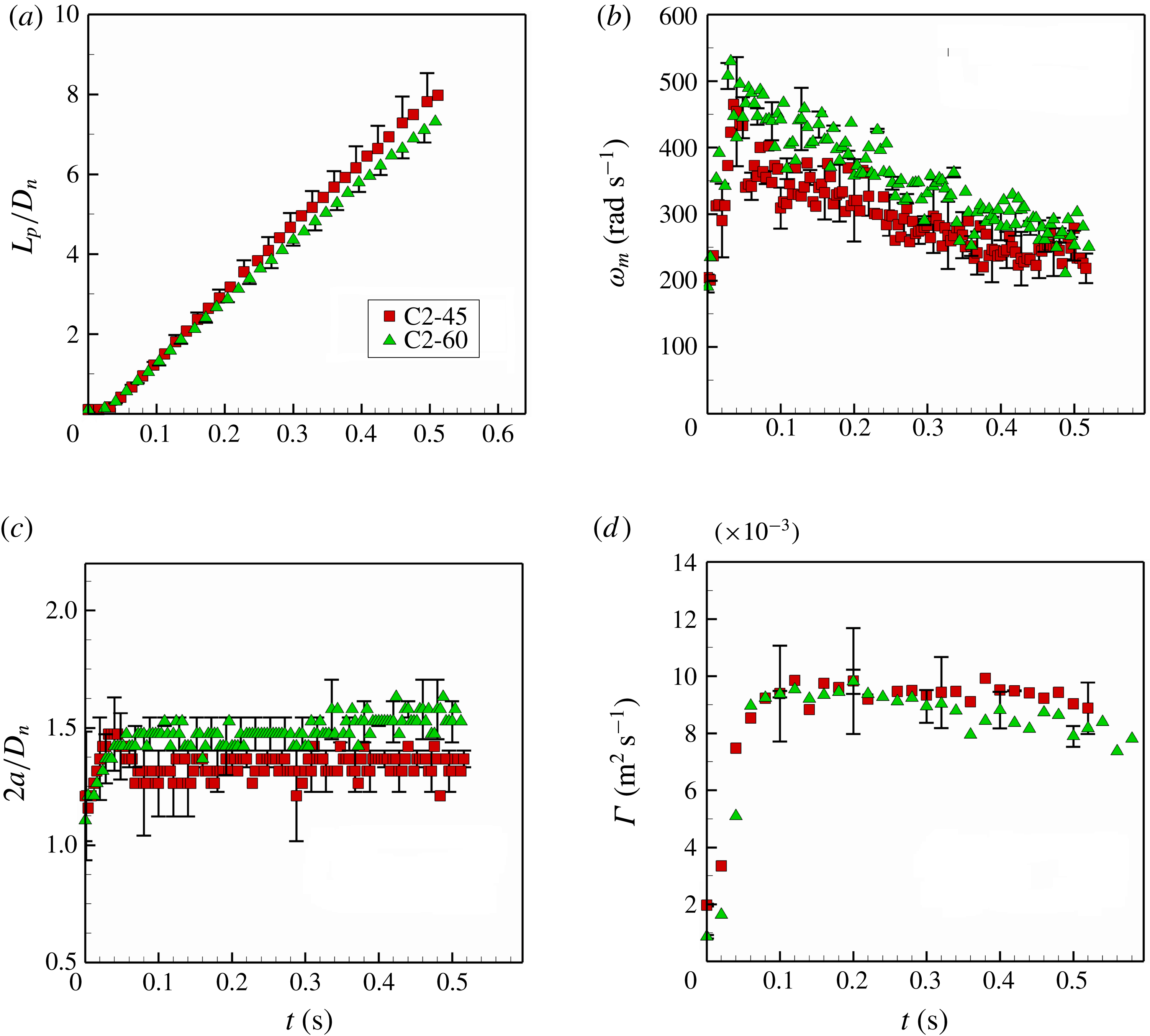
Figure 9 shows the variation in vortex parameters during their evolution for cases C2-45 and C2-60. The qualitative nature of the plots for both cases are almost similar. However, it is interesting to see that the vortex propagation velocity for C2-45 is marginally higher than C2-60. This may compel us to believe that C2-60 would carry lower vorticity values than C2-45. This is not evident from the plots (figure 9
b). On the contrary,
 $\unicode[STIX]{x1D714}_{max}$
values for C2-60 are significantly higher than C2-45. Moreover, vortex circulation values as shown in figure 9(d) are almost similar for both cases.
The observed phenomenon can only be explained provided the value of the standard deviation
 $\unicode[STIX]{x1D70E}$
for C2-60 is lower than for C1-45. However, this cannot be validated using our PIV data, due to high scatter. It can also be seen that the vortex spacing for C2-45 is consistently lower than for C2-60. This indicates a positive correlation between the vortex spacing and formation number ((
 $L/D_{n}$
) or (
 $V_{0}t_{0}/D_{n}$
)). This increased spacing may account for the lower translational velocity of C2-60. Such anomalous behaviour is also observed for the C1-45 and C1-60 cases.
In addition, it was most interesting to observe that the translational velocity for C3-45 was considerably higher than for C2-45, even though its peak vorticity values were significantly lower and the spacing
 $2a$
was higher than for C2-45. Insights into such counterintuitive behaviour are not addressed here and could form a topic of an altogether independent study. However, since this behaviour depends on vortex formation, we believe that it will be reflected in the vortex parameters (post-formation). It is expected that the dynamics of vortex evolution will not be affected provided that the vorticity variation is stable and follows a Gaussian distribution.
4.3 Comparison with theoretical predictions
Experimental results are used to validate the theoretical predictions offered in § 2. In view of this, we use optimization techniques to find a parameter that will best fit the vortex variables. MATLAB code was written to perform deterministic optimization by implementing the ‘gradient inversion’ technique, the details of which are given in appendix A. Using this technique, we calculate the best-fit parameter
 $\unicode[STIX]{x1D6FD}$
on a 60 % cropped experimental dataset of
 $\unicode[STIX]{x1D714}_{m}$
, where
 $\unicode[STIX]{x1D6FD}$
stands for
 $$\begin{eqnarray}\unicode[STIX]{x1D6FD}=\frac{2\unicode[STIX]{x1D719}\unicode[STIX]{x1D708}}{\unicode[STIX]{x1D70E}_{0}^{2}}.\end{eqnarray}$$
Consequent to evaluating the best-fit parameter using any one variable (here
 $\unicode[STIX]{x1D714}_{m}$
), we use this value to predict the variations in the other vortex parameters. We believe that the high accuracy of our predictions with other observed values should act as validators for the theory.
Using this approach, we have compared the measured values of vortex position (
 $L_{p}$
), peak vorticity (
 $\unicode[STIX]{x1D714}_{m}$
), sigma (
 $\unicode[STIX]{x1D70E}$
), circulation (
 $\unicode[STIX]{x1D6E4}$
) and vortex spacing (
 $2a$
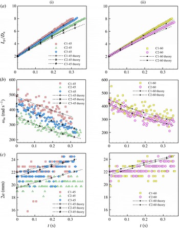
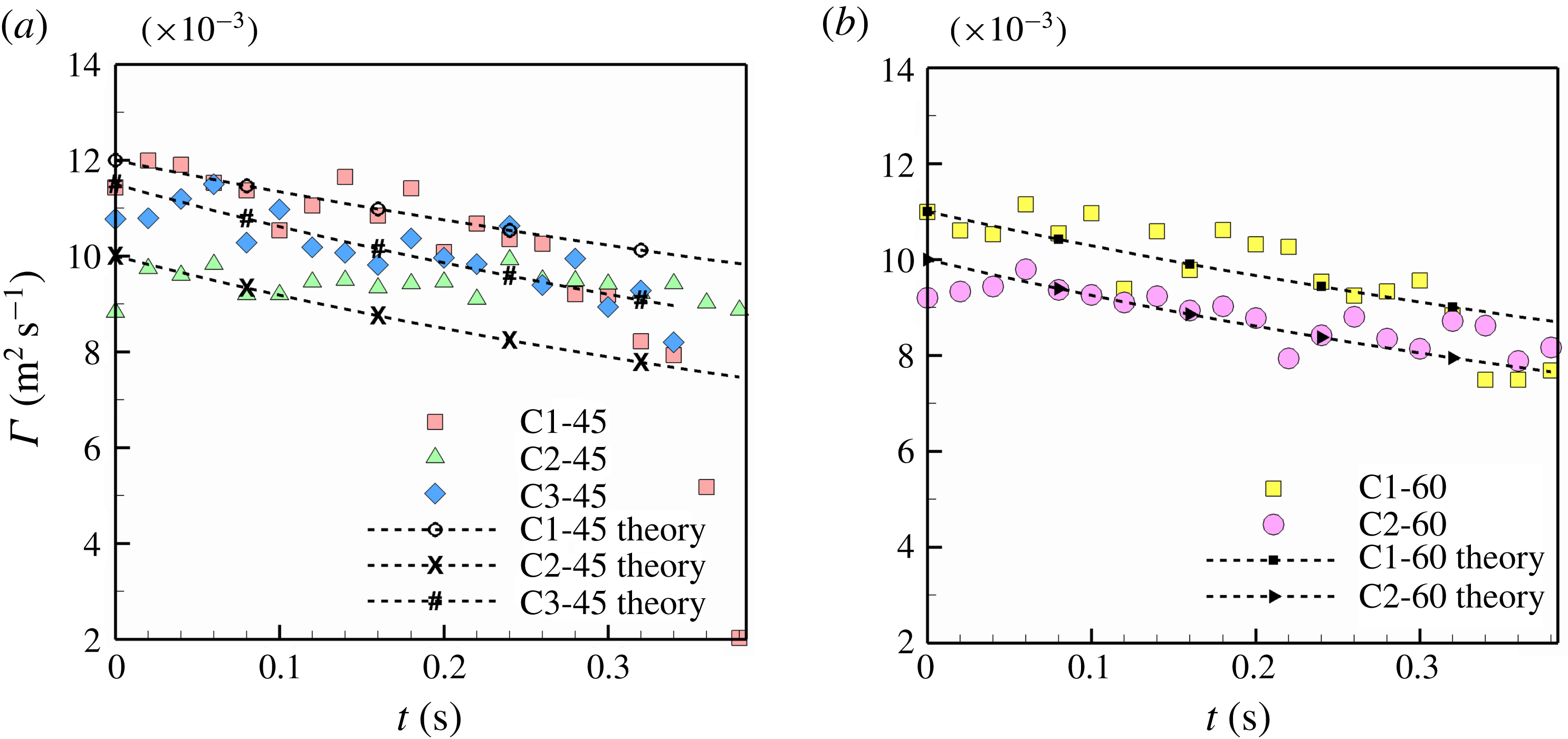
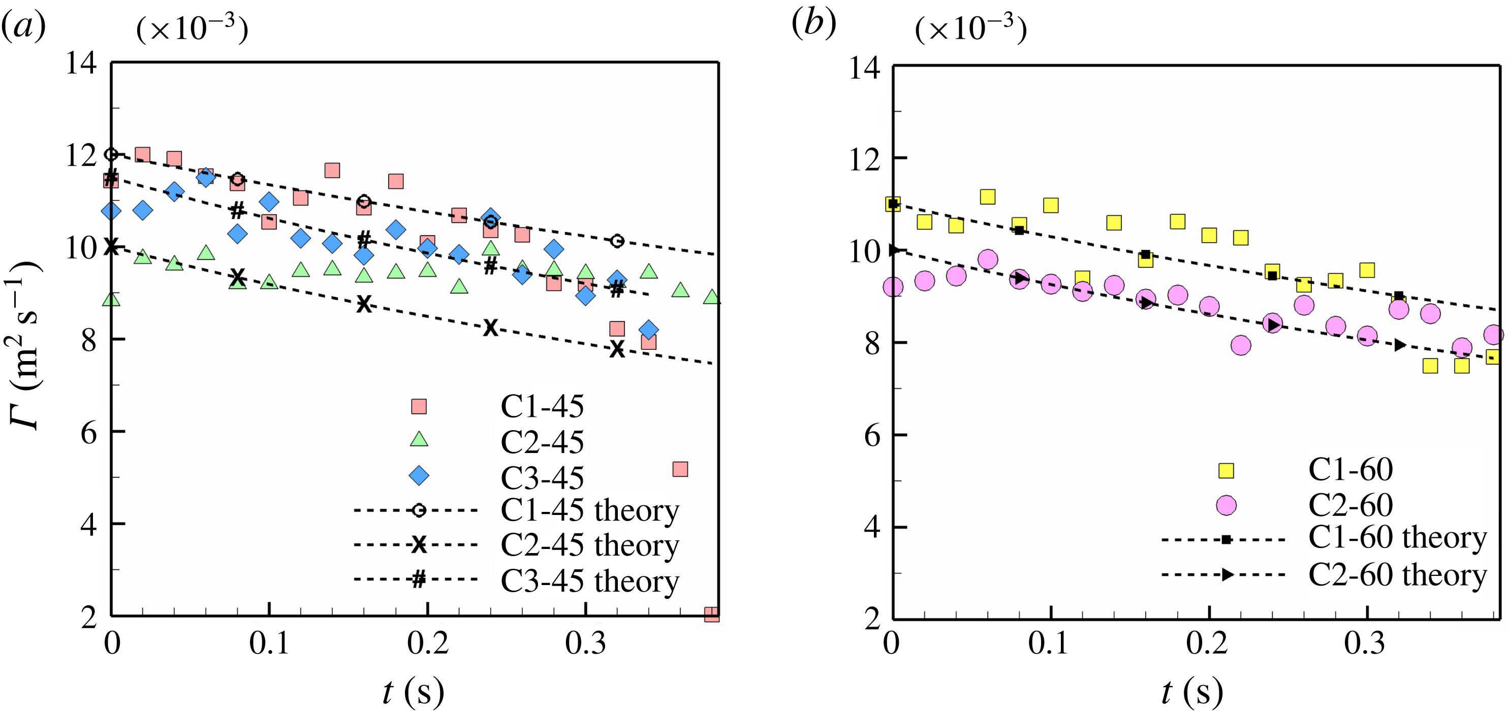
) with the values obtained using the theoretical equations (§ 2). The variations in these parameters along with the best-fit predictions are shown in figures 10 and 11.
Validation of experimental results with theory: (a)
 $L_{p}/D_{n}$
versus
 $t$
, (b)
 $\unicode[STIX]{x1D714}_{m}$
versus
 $t$
, (c)
 $2a$
versus
 $t$
.

It is worth mentioning that the value of
 $\unicode[STIX]{x1D6FD}$
obtained by the best fit of maximum vorticity leads to a near accurate estimate of the variation in the other parameters also. Even though good accuracy is obtained for the prediction of
 $\unicode[STIX]{x1D6E4}$
, high scatter is seen for
 $\unicode[STIX]{x1D70E}$
(not shown here) for the reasons explained in § 4.1. It is also visible that the theoretical predictions for vortex position are always lower than the experimentally observed values. Thus, it can be inferred that our theory underpredicts propagation velocities compared to experimentally observed values. Similarly, figure 10(c) also shows marginal overprediction for the vortex spacing (
 $2a$
). A detailed explanation regarding this behaviour is provided in § 5.2.
Validation of experimental results with theory:
 $\unicode[STIX]{x1D6E4}$
versus
 $t$
.
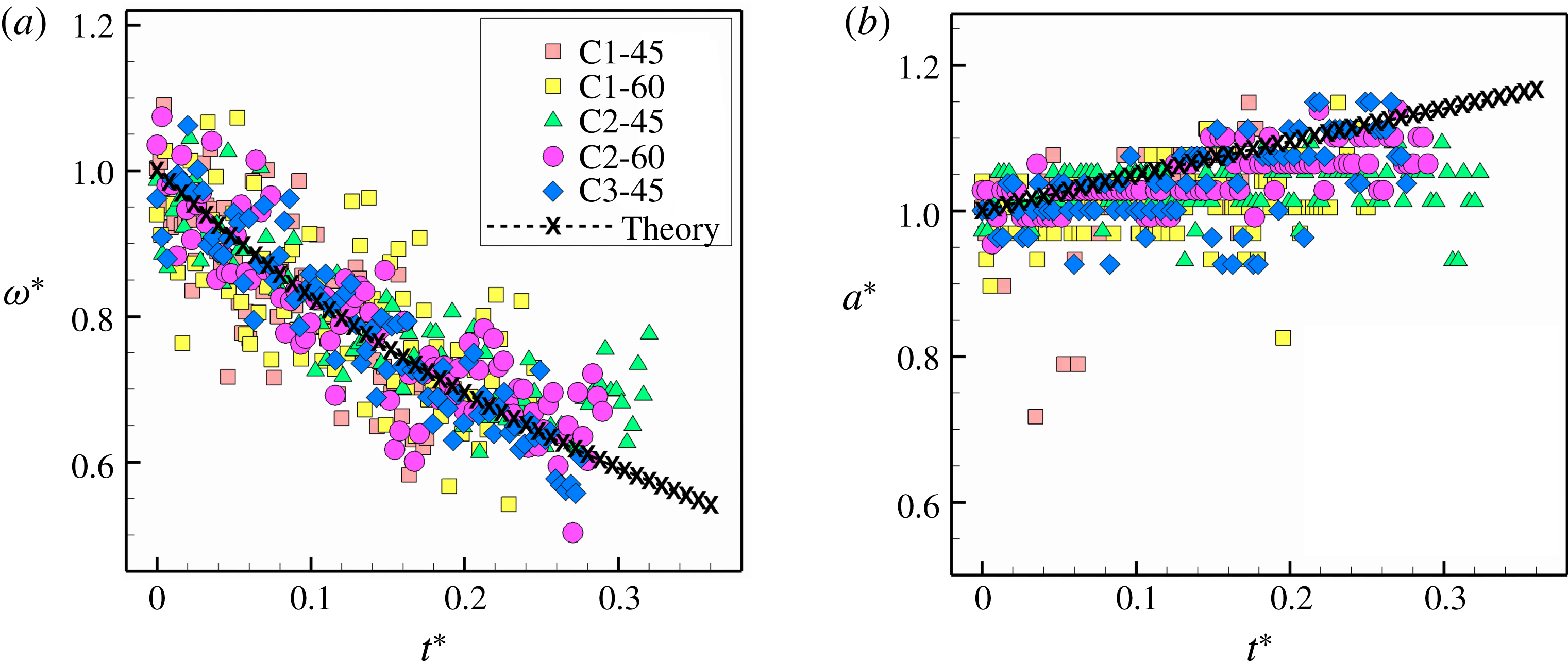
Non-dimensional forms of graphs for (a)
 $\unicode[STIX]{x1D714}^{\ast }$
versus
 $t^{\ast }$
and (b)
 $a^{\ast }$
versus
 $t^{\ast }$
.

All experimental cases have been compiled into combined plots (figure 12) using the non-dimensional form of (2.34) and (2.35). Thus, it can be seen that our theoretical model closely predicts vortex evolution in viscous fluids.
4.4 Comparison with available literature
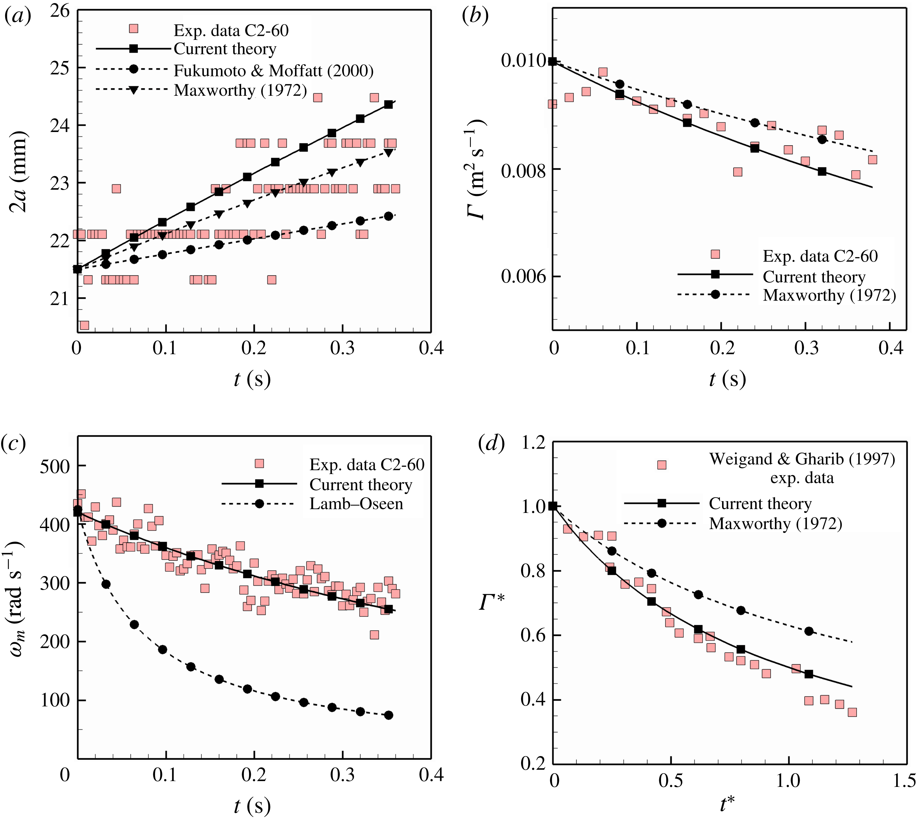
In order to test the effectiveness of our proposed theory, we have performed comparative studies on already existing experimental, numerical and analytical results. Figure 13(a) shows the variation in experimental and theoretical values of vortex spacing
 $2a$
for our case C2-60 and the respective predictions resulting from the analytical studies of Maxworthy (Reference Maxworthy1972) and Fukumoto & Moffatt (Reference Fukumoto and Moffatt2000) using (2.34) and (2.35). Corresponding data for the variation in circulation are also provided (figure 13
b). We see that the current theory provides a better match for observed values for the variation in circulation, whereas Maxworthy’s formula gives a better fit for the variation in vortex spacing
 $2a$
. In addition, the linear formula used by Fukumoto is seen to underpredict the expansion for C2-60.
Comparison of experimental values with existing theories: (a)
 $2a$
versus
 $t$
, (b)
 $\unicode[STIX]{x1D6E4}$
versus
 $t$
, (c)
 $\unicode[STIX]{x1D714}$
versus
 $t$
, (d) comparison with the experimental data of Weigand & Gharib (Reference Weigand and Gharib1997).
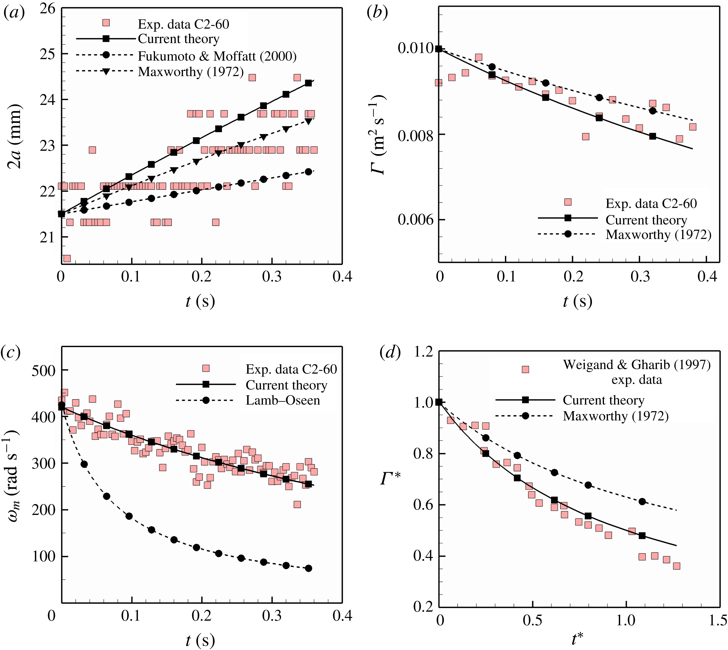
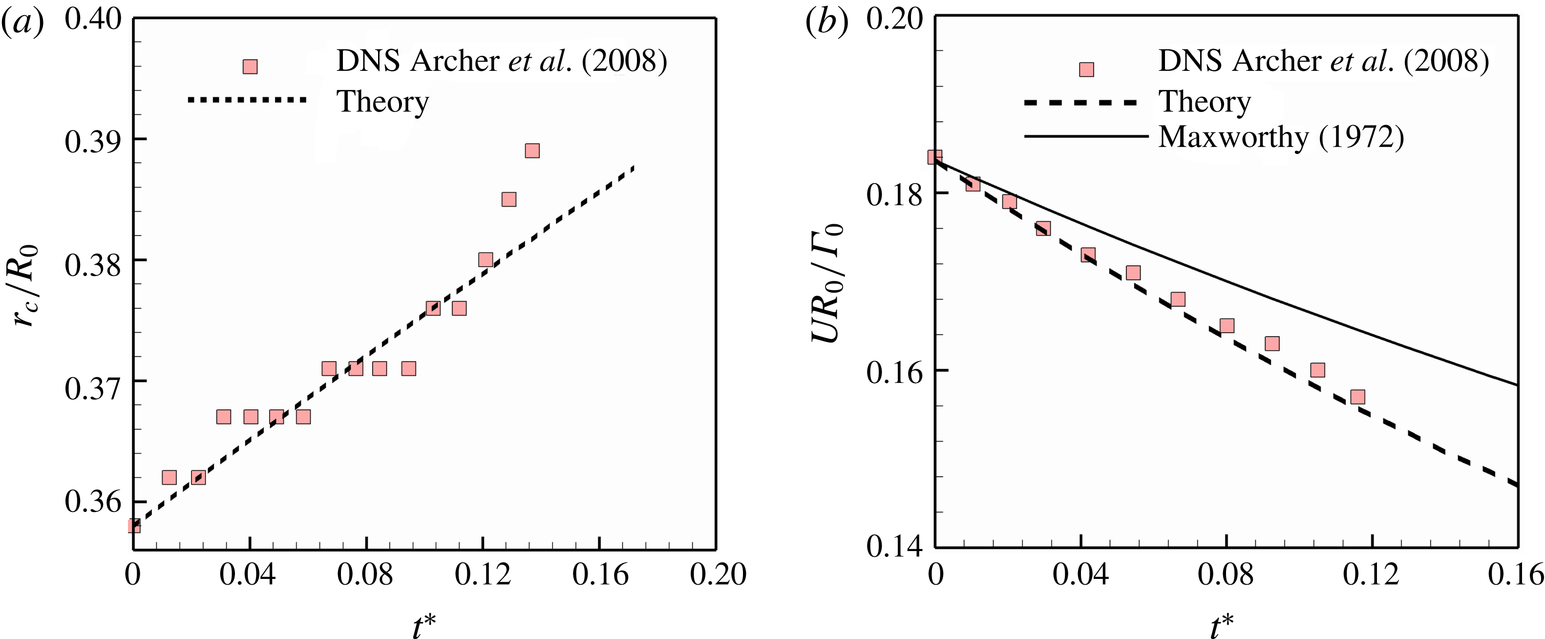
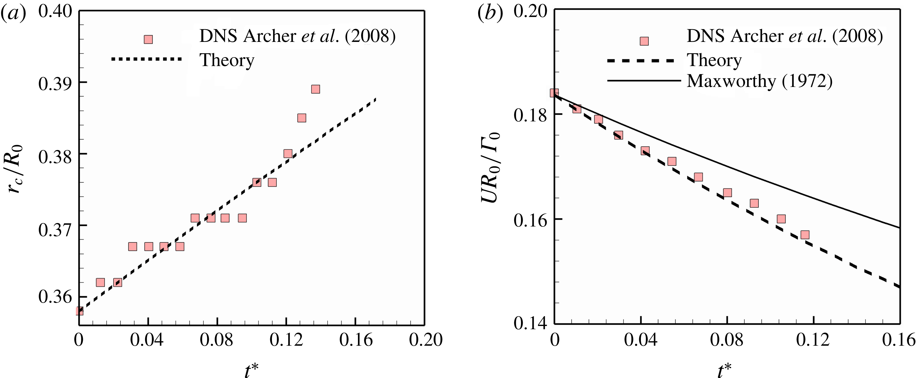
Figure 13(c) shows the variation in peak vorticity values for C2-60. It is interesting to note that the predictions from the Lamb–Oseen equation of vorticity (1.1) largely deviate from the observed values. This highlights the limited applicability of the Lamb–Oseen equation to short-time asymptotes only. In figure 13(d), we have used the experimental data of Weigand & Gharib (Reference Weigand and Gharib1997) to perform a comparative assessment of current theory with Maxworthy’s model. Moving forward, we have also tried to apply our theory to the DNS results of Archer, Thomas & Coleman (Reference Archer, Thomas and Coleman2008). Plots in figure 14 show the variation in non-dimensional forms of core radius and translational velocity for
 $Re=5500$
and slenderness ratio (
 $r_{c}/a=0.4$
). Using the best-fit approach, it can be seen that the proposed theory offers a better prediction of the observed dynamics.
It is necessary to mention that such studies have proved to be challenging. Many of the prior studies have rarely focused their attention on the vorticity distribution or precise core size, which forms an important parameter in our predictive theory. Moreover, the above comparisons have been conducted for practically thick vortex rings in the Reynolds number range 77–5500. Studies pertaining to thin rings have not been compared, primarily due to the scarcity of experimental results in this regime.
Fitting of our theory into the DNS data of Archer et al. (Reference Archer, Thomas and Coleman2008): (a) core size versus time, and (b) velocity versus time.
However, short asymptotic studies have proposed relations for the vortex propagation velocity which carry a completely different functional relationship with time. Saffman’s equation claims a dependence relation of
 $-\text{log}(\unicode[STIX]{x1D708}t)$
, which is different from the relation
 $t^{-3/2}$
as concluded by current theory. Thus, we believe that the theory, in its current form, offers good insights into the medium–large-time regimes of vortex lifetimes, although it performs unsatisfactorily in the lower asymptotic limits. This subject is further discussed in § 5.
4.5 Interpretations from the derived values of
 $\unicode[STIX]{x1D6FD}$
,
$k_{1}$


Using the best-fit value of
 $\unicode[STIX]{x1D6FD}$
for each case, combined with measured values of
 $\unicode[STIX]{x1D70E}_{0}$
and
 $\unicode[STIX]{x1D708}$
, we have calculated the averaging parameter
 $\unicode[STIX]{x1D719}$
, and thereby
 $k_{1}$
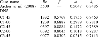
using the relation (2.19). These results are compiled in table 2.
 $\unicode[STIX]{x1D6FD}$
is the only adjustable parameter in our theoretical model. Errors in
 $\unicode[STIX]{x1D6FD}$
are sensitive to errors in the measurement of
 $\unicode[STIX]{x1D714}_{m}$
and the standard deviation
 $\unicode[STIX]{x1D70E}$
(4.1). Considering the PIV resolution, the net accumulated error in
 $\unicode[STIX]{x1D6FD}$
is approximately 10 %–12 %. Since
 $\unicode[STIX]{x1D719}$
is highly sensitive to changes in
 $k_{1}$
(2.19), the net error in
 $k_{1}$
translates to not more than 2 %–3 %.
Results table with parameter values for each case.
Note that the value of
 $\unicode[STIX]{x1D6FD}$
is obtained from curve fitting, and no mathematical relations have been provided. Similarly, our mathematical model did not specify the vortex core parameter
 $k_{1}$
that is to be used. This is because we believe that the vortex core parameter that is to be used for proper averaging is a complex function of vorticity distribution and fluid properties which is non-trivial to guess beforehand and would require separate dedicated efforts. Nevertheless, our approach provides important insights. It is observed (table 2) that the value of
 $k_{1}>0.707$
for our test cases, and approaches (
 $1/\sqrt{2}$
) for decreasing Reynolds numbers. In case of low-Reynolds-number vortex rings, which have considerably thick vortex cores (vorticity distribution extending up to centreline, as in the fat-limit case of Hill’s spherical vortex (Maxworthy Reference Maxworthy1972; Hill Reference Hill1894)), we see that our theory predicts a
 $k_{1}$
value that is consistent with the available literature. In such cases, the core size
 $\unicode[STIX]{x1D716}$
will be given by
 $(k_{1}\unicode[STIX]{x1D70E})\approx (k_{1}\times a)=(a/\sqrt{2})$
, which equals the proposed value of slenderness ratio for Hill’s spherical vortex. Thus, our model seamlessly integrates with established theories.
Although the best-fit approach provides validation for our proposed theory, understanding the nature of variation in
 $k_{1}$
is necessary to transform it into a predictive and deterministic tool.
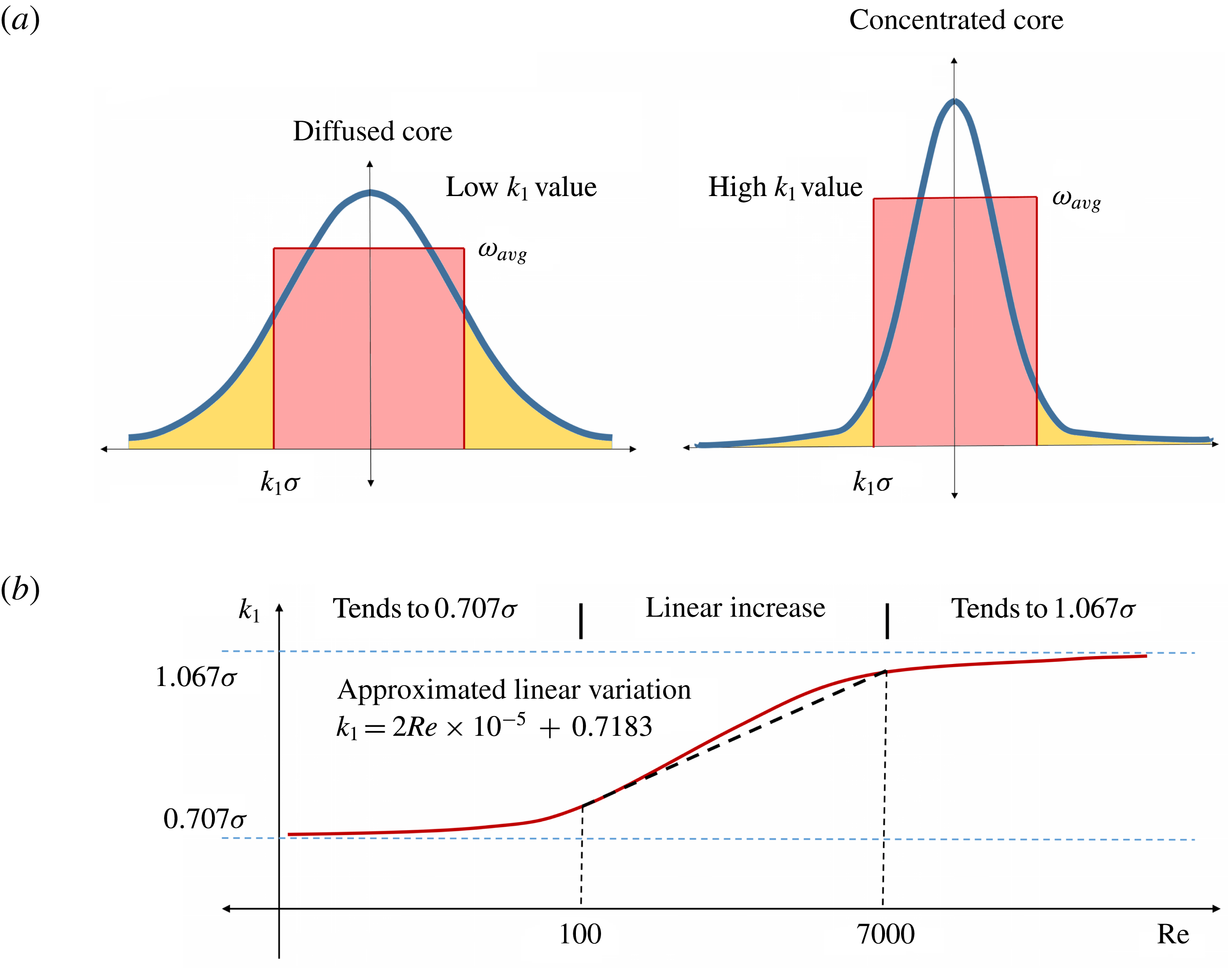
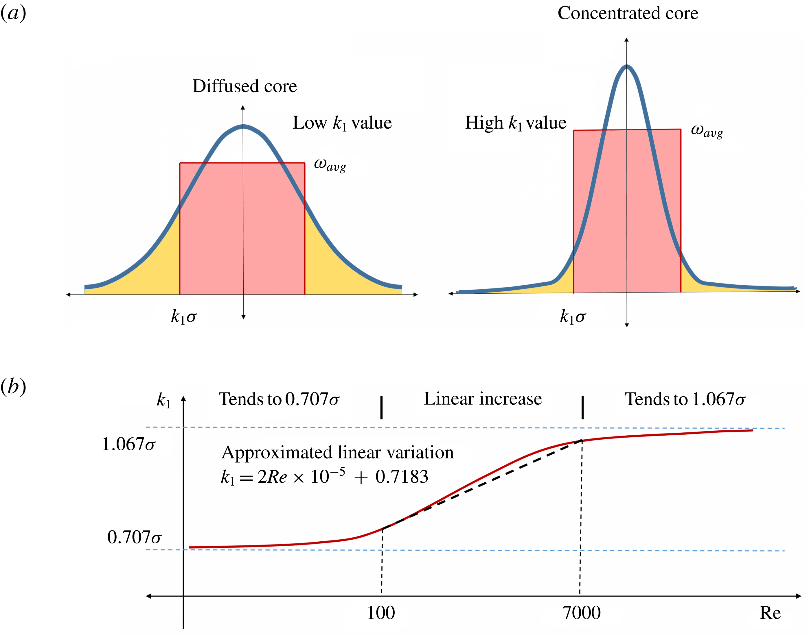
(a) Schematic showing the physical importance of the vorticity profile on the selection of the
 $k_{1}$
values. (b) Approximate variation in
 $k_{1}$
values w.r.t. Reynolds number.
The variation in
 $k_{1}$
can be best analysed by understanding the physical role it plays in deriving the theory in § 2.
 $k_{1}$
is taken to be the radius of a hypothetical disc with constant average vorticity which best mimics the vorticity diffusion (figure 15
a). Under this assumption, internal viscous interactions are neglected, thereby reducing the problem to that of external viscous diffusion only. Further, it can be intuitively understood that a core with high circulation will largely behave as a solid disc with negligible internal dissipation compared to external dissipative effects. Thus, Reynolds number plays a significant role in realizing
 $k_{1}$
values.
Our observations provide us with a lower bound of
 $k_{1}$
which approaches (
 $1/\sqrt{2}$
) as
 $Re\rightarrow \infty$
, which makes
 $\unicode[STIX]{x1D719}\rightarrow 0$
and results in negligible relative vorticity diffusion, as can be seen in (2.24). On the other end, as
 $Re\rightarrow \infty$
, we predict that the value of
 $k_{1}$
should be such that it maximizes
 $\unicode[STIX]{x1D719}$
, leading to the maximum relative viscous dissipation. Using trial and error methods, we arrive at a value approximately equal to 1.067. This forms the higher asymptotic limit of
 $k_{1}$
. Thus, the variation in
 $k_{1}$
with respect to Reynolds number can be best described by a curve as shown in figure 15(b).
In the moderate
 $Re$
range (100–10 000), variation in
 $k_{1}$
can be approximated to be linear. From our obtained values (table 2), this linear trend can be quantified by the following equation;
 $$\begin{eqnarray}k_{1}=2Re\times 10^{-5}+0.7183.\end{eqnarray}$$
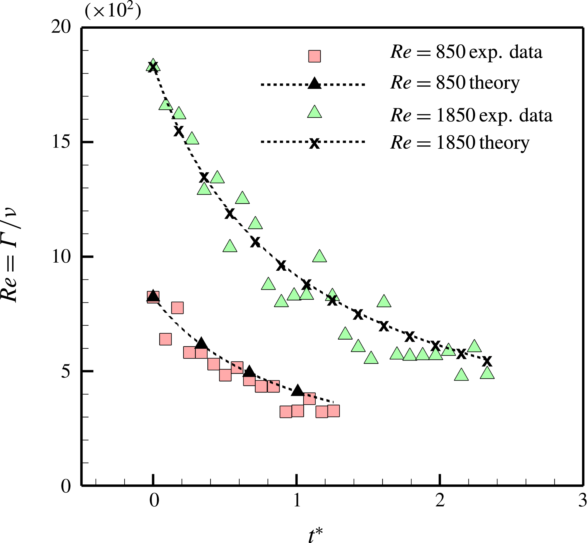
Fitting our theory on experimental data; non-dimensional circulation versus non-dimensional time.
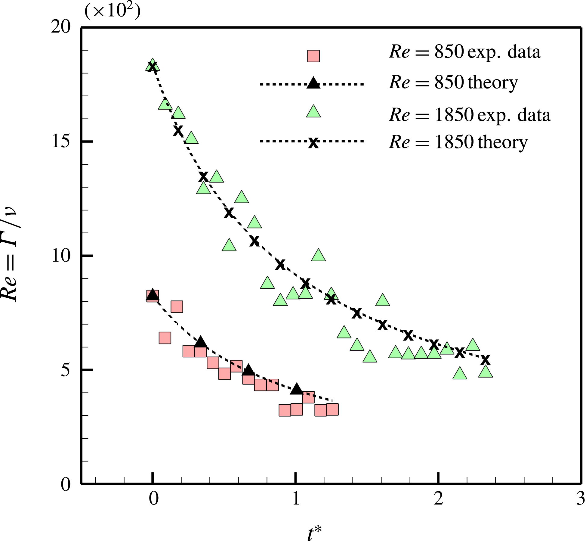
Validation of the above equation has been attempted by comparing the same with the experimental results of Dziedzic & Leutheusser (Reference Dziedzic and Leutheusser1996). The theoretical trend shown in figure 16, obtained using (4.2), shows good agreement with the experimental values.
5 Discussions
5.1 Differences between current theory and the Lamb–Oseen equation
The classic equation for vorticity diffusion (1.1), widely accepted for understanding vortex evolution in viscous fluids, was given by Lamb–Oseen (Oseen Reference Oseen1910; Lamb Reference Lamb1932):
 $$\begin{eqnarray}\unicode[STIX]{x1D714}(r,t)=\frac{\unicode[STIX]{x1D6E4}_{0}}{4\unicode[STIX]{x03C0}\unicode[STIX]{x1D708}t}\text{e}^{-(r^{2}/4\unicode[STIX]{x1D708}t)}.\end{eqnarray}$$
This equation was carefully derived assuming constant circulation. It is based on the argument that viscosity causes vorticity to diffuse out of the fixed contour. However, for smaller times, this effect is negligible. Thus, for short times, when the entire vorticity can be assumed to remain contained within the core, (1.1) has been accepted to provide good insights into vortex evolution. Also, it is explained that, for larger times, the vorticity diffuses and cancels itself at the vortex centreline, thus invalidating the assumption of constant circulation. Therefore, studies have shown that the Lamb–Oseen equation provides good insight into the dynamics of thin-core vortices at very short times, but it fails to explain the evolution of rings even with moderate slenderness ratio. These differences can be explained in the following way.
Consider a vortex monopole with the vorticity distribution given by (1.1), as shown in figure 2. For such a vortex the total circulation throughout the domain remains constant. This is a direct result of the constant circulation assumption used for deriving (1.1)
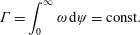 $$\begin{eqnarray}\unicode[STIX]{x1D6E4}=\int _{0}^{\infty }\unicode[STIX]{x1D714}\,\text{d}\unicode[STIX]{x1D713}=\text{const}.\end{eqnarray}$$
Such viscous interactions are governed by the laws of conservation of angular momentum. For 2D cases, this results in the expression given below:
 $$\begin{eqnarray}I=\int \unicode[STIX]{x1D714}\,\text{d}I\propto \unicode[STIX]{x1D6E4}r^{2}=\text{const}.\end{eqnarray}$$
This suggests that circulation does not remain conserved even when calculated throughout the domain, but in fact decreases due to the addition of bulk fluid. Circulation reduction in a finite-size contour is thus a result of the superposition of two phenomena: (i) vorticity diffusion out of the contour and (ii) an increase in the vortex size.
We have used the above conservation principle to frame the proposed theory. No doubt the theory shows important differences with respect to that of Lamb–Oseen. It predicts a reduction in circulation values, which is indeed observed in our experiments.
5.2 Insights into ring expansion and integration of short- and long-time behaviour
Using our graphs (figures 10 and 11) depicting the variation in
 $V^{\ast }$
versus
 $t^{\ast }$
, it can be seen that the values obtained from our experimental studies show a variation with respect to theoretical predictions. Similar differences were reported by Maxworthy (Reference Maxworthy1972). Moreover, it can be observed that this deviation between experimental values and theoretical predictions is relatively lower for low-
 $Re$
cases, and increases with an increase in the vortex Reynolds number. It is also worthwhile mentioning that similar discrepancies are also noticeable in the variation of the vortex ring radius
 $a^{\ast }$
. However, this mismatch seen in
 $V^{\ast }$
and
 $a^{\ast }$
with respect to
 $t^{\ast }$
is not reflected in the graphs for the variation of
 $\unicode[STIX]{x1D714}^{\ast }$
or
 $\unicode[STIX]{x1D6E4}^{\ast }$
. Thus, the observed phenomenon directs us to infer that the vorticity diffusion behaviour and consequent entrainment rates are largely governed by viscous effects only. However, the vortex translational velocity gradient and ring expansion are sensitive to Reynolds numbers.
This observed mismatch is somewhat logical if we consider the velocity–spacing coupling for vortex rings. For the Lamb–Oseen vortex (example), Saffman (Reference Saffman1970) predicted the following velocity equation:
 $$\begin{eqnarray}V=\frac{\unicode[STIX]{x1D6E4}_{0}}{4\unicode[STIX]{x03C0}a_{0}}\left[\ln \left(\frac{8a_{0}}{\sqrt{4\unicode[STIX]{x1D708}t}}\right)-0.558\right].\end{eqnarray}$$
Thus, an overprediction related to vortex spacing
 $a$
will reflect in lower theoretical values for the corresponding translational velocity. Fukumoto & Moffatt (Reference Fukumoto and Moffatt2000) performed rigorous mathematical studies to understand the time evolution of the vortex spacing
 $a$
and propagation velocity
 $V$
. He obtained equations equivalent to (1.5) and (1.4). He attributed vortex ring expansion solely to viscous effects, which he put forward as linearly dependent on
 $\unicode[STIX]{x1D708}$
and independent of
 $\unicode[STIX]{x1D6E4}$
. Though he was successful in gathering qualitative validation for his claims through comparison with already published results (Oshima Reference Oshima1972; Watanabe et al.
Reference Watanabe, Nakamichi, Jang, Kazama, Hasegawa and Ishiwata1995; Wakelin & Riley Reference Wakelin and Riley1997), he could not provide any quantitative validation. For higher Reynolds numbers his proposed linear relation failed, and highly overestimated vortex ring expansion.
Experiments conducted by Weigand & Gharib (Reference Weigand and Gharib1997) show similar characteristics. They used a best-fit parameter in Saffman’s equations (Saffman Reference Saffman1970) and observed that the translational velocity scales with (1.2) for shorter times, but shifts to (1.5) at larger times. This observation was also cross-validated by the numerical values of Stanaway et al. (Reference Stanaway, Cantwell and Spalart1988). This aspect is studied in a whole new perspective in the recent work of Sullivan et al. (Reference Sullivan, Niemela, Hershberger, Bolster and Donnelly2008). In their exhaustive work, they compared their experimental data with published results. They concluded that, for thin vortex rings as generated in their experiments, vortex slowdown was primarily due to circulation reduction caused by hydrodynamic drag forces. However, they did not observe and account for the expected increase in core size and ring diameters.
Though these universal behaviours have been reported on numerous occasions, no physical insights into the transition of velocity profiles have been presented yet. Many comprehensive studies have elucidated the hydrodynamic mechanism governing the one-dimensional axial velocity variation of vortex rings. In contrast, relations for the variation in vortex spacing have been, most of the times, derived using dimensional analysis. Using dynamical equations of force balance, we try to explain this behaviour in more detail.
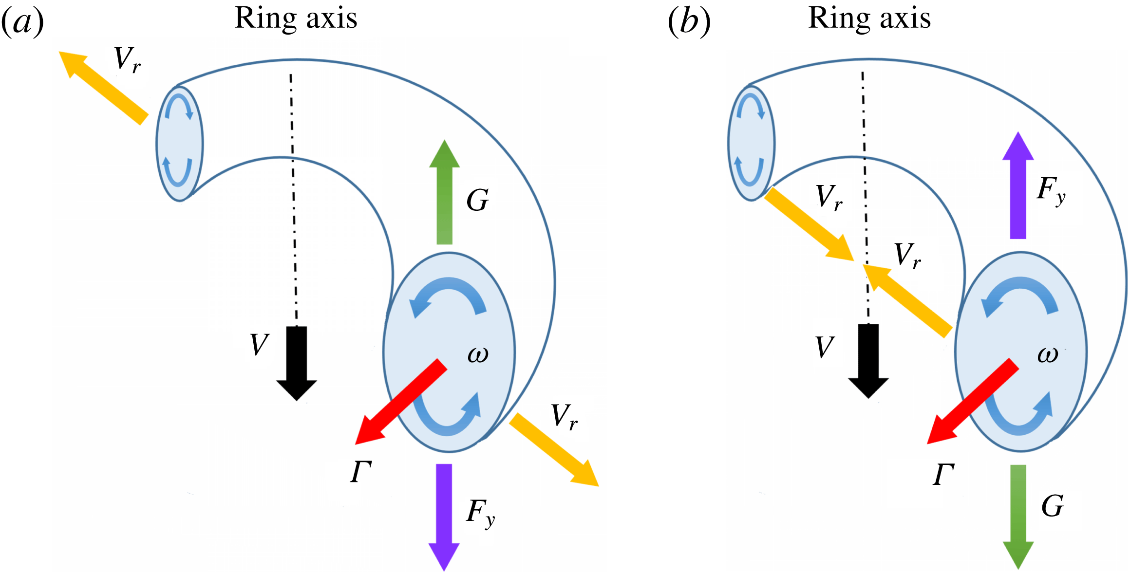
Forces on vortex rings: (a) during entrainment, (b) during detrainment.
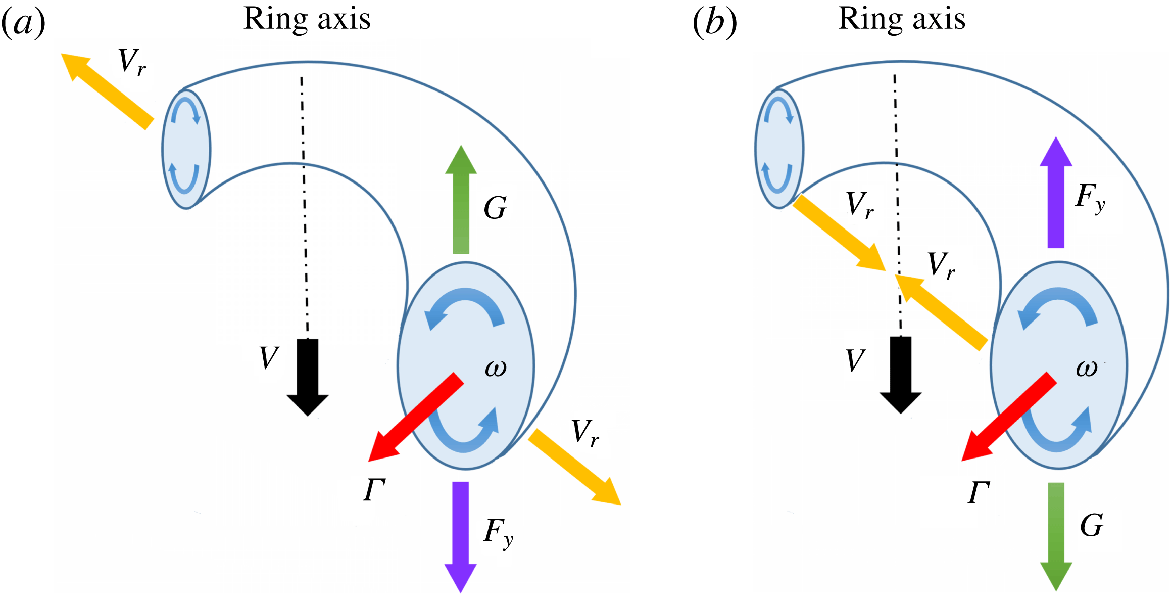
Variation in the vortex spacing
 $2a$
describes the radial displacement of the vorticity centre w.r.t. the axis of the vortex ring. For a vortex ring (figure 17) propagating in an isodensity fluid, and entraining mass on its way, it is under the influence of various forces: namely (i) the drag force opposing the vortex motion, (ii) the body force
 $\boldsymbol{F}_{y}$
acting in the axial direction, and (iii) the Magnus force
 $\boldsymbol{G}$
. Of these, the effect of the drag force is negligible compared to the effect of increasing mass and spacing due to diffusion and circulation, respectively. For such vortex rings, the body force can be given by
 $$\begin{eqnarray}\boldsymbol{F}_{\boldsymbol{y}}\approx \boldsymbol{V}\frac{\text{d}m}{\text{d}t}.\end{eqnarray}$$
Thus, for the rate of entrained mass to be positive, the body force acts in the direction of vortex motion. Using Newton’s second law, we arrive at the dynamic equation for the vortex ring, given by
 $$\begin{eqnarray}\boldsymbol{F}_{\boldsymbol{y}}+\boldsymbol{G}=m\frac{\text{d}\boldsymbol{V}}{\text{d}t}.\end{eqnarray}$$
However, for small values of mass and velocity variation, the
 $\text{right-hand side}\rightarrow 0$
, and hence
 $$\begin{eqnarray}\boldsymbol{F}_{\boldsymbol{y}}=-\boldsymbol{G}.\end{eqnarray}$$
The Magnus force
 $\boldsymbol{G}$
is opposite to the body force
 $\boldsymbol{F}_{y}$
and equal in magnitude. This force
 $\boldsymbol{G}$
over a vortex ring of radius
 $a$
is mathematically given by
 $$\begin{eqnarray}\boldsymbol{G}=(2\unicode[STIX]{x03C0}a)\unicode[STIX]{x1D70C}(\unicode[STIX]{x1D71E}\times \boldsymbol{V}_{\boldsymbol{r}}),\end{eqnarray}$$
where
 $\boldsymbol{V}_{r}$
is the radial expansion velocity of the vortex ring, equal to
 $(\text{d}a/\text{d}t)$
. From (5.5), (5.7) and (5.8) we arrive at an expression for the radial velocity, given by
 $$\begin{eqnarray}|\boldsymbol{V}_{\boldsymbol{r}}|=\frac{\text{d}\boldsymbol{a}}{\text{d}t}=\frac{1}{2\unicode[STIX]{x03C0}\unicode[STIX]{x1D70C}a\unicode[STIX]{x1D6E4}}\times \left|\boldsymbol{V}\frac{\text{d}m}{\text{d}t}\right|.\end{eqnarray}$$
A similar approach was used (Rayfield & Reif Reference Rayfield and Reif1964; Sonin Reference Sonin2016) to study the dynamical properties of quantized charge-carrying vortex rings, moving in superfluid Helium at low temperatures, where the quantum of circulation was found to be equal to
 $h/m$
, where
 $h$
is Planck’s constant and
 $m$
is the mass of the Helium atom.
Thus, it can be observed that, when a vortex entrains fluid
 $(\text{d}m/\text{d}t>0)$
, the body force
 $\boldsymbol{F}_{y}$
acts in the direction of the vortex velocity and the radial velocity
 $\boldsymbol{V}_{r}$
points in the outward direction, leading to an increase in the ring diameter (vortex spacing in case of two dimensions). The opposite phenomenon is observed when detrainment occurs, as in case when the vortex penetrates a stratified medium. As the vortex penetrates through a higher density and higher viscosity fluid, viscous and buoyancy forces result in peeling of the vortex mass
 $(\text{d}m/\text{d}t<0)$
. In such cases,
 $\boldsymbol{F}_{y}$
acts opposite to the axial velocity and
 $\boldsymbol{V}_{r}$
should point inwards, leading to a collapse of the vortex rings.
The above approach can be extended further to understand the qualitative as well as quantitative aspects of vortex ring evolution. For a toroidal vortex ring with circular cross-section, as shown in figure 1, with core radius
 $R$
, the mass of the ring can be given as
 $$\begin{eqnarray}m=\unicode[STIX]{x1D70C}(2\unicode[STIX]{x03C0}^{2}aR^{2}).\end{eqnarray}$$
Thus, for non-buoyant vortex rings, where the vortex density is unaltered due to entrainment effects, the rate of change of vortex mass is given by
 $$\begin{eqnarray}\frac{\text{d}m}{\text{d}t}=2\unicode[STIX]{x03C0}^{2}\left[R^{2}\frac{\text{d}a}{\text{d}t}+2aR\frac{\text{d}R}{\text{d}t}\right].\end{eqnarray}$$
Thus, equation (5.9) can be represented as
 $$\begin{eqnarray}\left|\boldsymbol{V}_{\boldsymbol{r}}\right|=\frac{\text{d}a}{\text{d}t}=\frac{1}{2\unicode[STIX]{x03C0}\unicode[STIX]{x1D70C}a\unicode[STIX]{x1D6E4}}|\boldsymbol{V}|2\unicode[STIX]{x03C0}^{2}\unicode[STIX]{x1D70C}\left[R^{2}\frac{\text{d}a}{\text{d}t}+2aR\frac{\text{d}R}{\text{d}t}\right].\end{eqnarray}$$
After some manipulations, we arrive at a simplified implicit relation given by
 $$\begin{eqnarray}\frac{\text{d}a}{\text{d}t}=\frac{2\unicode[STIX]{x03C0}R|\boldsymbol{V}|}{\unicode[STIX]{x1D6E4}\displaystyle \left\{1-\frac{\unicode[STIX]{x03C0}|\boldsymbol{V}|R^{2}}{\unicode[STIX]{x1D6E4}a}\right\}}\frac{\text{d}R}{\text{d}t}.\end{eqnarray}$$
However, for vortex rings, with the simplifying assumption that the entire circulation is distributed evenly in a finite core of radius
 $R$
, the centreline velocity can be given by
 $|\boldsymbol{V}|=(\unicode[STIX]{x1D6E4}/4\unicode[STIX]{x03C0}a)$
. This simplifies the above equation to give
 $$\begin{eqnarray}\frac{\text{d}a}{\text{d}t}=\frac{\displaystyle 2\left(\frac{R}{a}\right)}{\displaystyle \left\{4-\left(\frac{R}{a}\right)^{2}\right\}}\frac{\text{d}R}{\text{d}t}.\end{eqnarray}$$
If we consider the vortex core radius
 $R=\unicode[STIX]{x1D709}\unicode[STIX]{x1D70E}$
, where
 $\unicode[STIX]{x1D709}$
is a numerical constant determining the extent of the vortex core and
 $\unicode[STIX]{x1D70E}$
is the standard deviation of the Gaussian vorticity distribution as shown in figure 3, we can write from our result (2.24)
 $$\begin{eqnarray}\frac{\text{d}R}{\text{d}t}=\unicode[STIX]{x1D709}\frac{\text{d}\unicode[STIX]{x1D70E}}{\text{d}t}=\unicode[STIX]{x1D709}\frac{\displaystyle \left(\frac{2\unicode[STIX]{x1D719}\unicode[STIX]{x1D708}}{\unicode[STIX]{x1D70E}_{0}}\right)}{\displaystyle 2\sqrt{1+\frac{2\unicode[STIX]{x1D719}\unicode[STIX]{x1D708}t}{\unicode[STIX]{x1D70E}_{0}^{2}}}}.\end{eqnarray}$$
Substituting this in (5.14), we get
 $$\begin{eqnarray}\frac{\text{d}a}{\text{d}t}=\frac{\displaystyle \left(\frac{\unicode[STIX]{x1D709}\unicode[STIX]{x1D70E}}{2a}\right)}{\displaystyle \left\{1-\frac{(\unicode[STIX]{x1D709}\unicode[STIX]{x1D70E})^{2}}{4a^{2}}\right\}}\frac{\text{d}R}{\text{d}t}=\frac{\displaystyle \left(\frac{\unicode[STIX]{x1D709}\unicode[STIX]{x1D70E}}{2a}\right)}{\displaystyle \left\{1-\frac{(\unicode[STIX]{x1D709}\unicode[STIX]{x1D70E})^{2}}{4a^{2}}\right\}}\times \unicode[STIX]{x1D709}\frac{\displaystyle \left(\frac{2\unicode[STIX]{x1D719}\unicode[STIX]{x1D708}}{\unicode[STIX]{x1D70E}_{0}}\right)}{\displaystyle 2\sqrt{1+\frac{2\unicode[STIX]{x1D719}\unicode[STIX]{x1D708}t}{\unicode[STIX]{x1D70E}_{0}^{2}}}},\end{eqnarray}$$
where, substituting the relation for
 $\unicode[STIX]{x1D70E}$
gives us
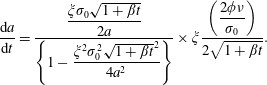 $$\begin{eqnarray}\frac{\text{d}a}{\text{d}t}=\frac{\displaystyle \frac{\unicode[STIX]{x1D709}\unicode[STIX]{x1D70E}_{0}\sqrt{1+\unicode[STIX]{x1D6FD}t}}{2a}}{\displaystyle \left\{1-\frac{\unicode[STIX]{x1D709}^{2}\unicode[STIX]{x1D70E}_{0}^{2}\sqrt{1+\unicode[STIX]{x1D6FD}t}^{2}}{4a^{2}}\right\}}\times \unicode[STIX]{x1D709}\frac{\displaystyle \left(\frac{2\unicode[STIX]{x1D719}\unicode[STIX]{x1D708}}{\unicode[STIX]{x1D70E}_{0}}\right)}{\displaystyle 2\sqrt{1+\unicode[STIX]{x1D6FD}t}}.\end{eqnarray}$$
Here
 $\unicode[STIX]{x1D6FD}$
is a temporary variable given by
 $(2\unicode[STIX]{x1D719}\unicode[STIX]{x1D708}/\unicode[STIX]{x1D70E}_{0}^{2})$
. After cancellation of common terms, the above equation reduces to
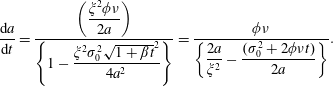 $$\begin{eqnarray}\frac{\text{d}a}{\text{d}t}=\frac{\displaystyle \left(\frac{\unicode[STIX]{x1D709}^{2}\unicode[STIX]{x1D719}\unicode[STIX]{x1D708}}{2a}\right)}{\displaystyle \left\{1-\frac{\unicode[STIX]{x1D709}^{2}\unicode[STIX]{x1D70E}_{0}^{2}\sqrt{1+\unicode[STIX]{x1D6FD}t}^{2}}{4a^{2}}\right\}}=\frac{\unicode[STIX]{x1D719}\unicode[STIX]{x1D708}}{\displaystyle \left\{\frac{2a}{\unicode[STIX]{x1D709}^{2}}-\frac{(\unicode[STIX]{x1D70E}_{0}^{2}+2\unicode[STIX]{x1D719}\unicode[STIX]{x1D708}t)}{2a}\right\}}.\end{eqnarray}$$
This equation can then be solved in the following manner,
 $$\begin{eqnarray}\displaystyle & \displaystyle \frac{2a}{\unicode[STIX]{x1D709}^{2}}\,\text{d}a-\frac{(\unicode[STIX]{x1D70E}_{0}^{2}+2\unicode[STIX]{x1D719}\unicode[STIX]{x1D708}t)}{2a}\,\text{d}a=\unicode[STIX]{x1D719}\unicode[STIX]{x1D708}\,\text{d}t. & \displaystyle\end{eqnarray}$$
 $$\begin{eqnarray}\displaystyle & \displaystyle \int \frac{2a^{2}}{\unicode[STIX]{x1D709}^{2}}\,\text{d}a-\int \frac{\unicode[STIX]{x1D70E}_{0}^{2}}{2}\,\text{d}a=\int (\unicode[STIX]{x1D719}\unicode[STIX]{x1D708}a\,\text{d}t+\unicode[STIX]{x1D719}\unicode[STIX]{x1D708}t\,\text{d}a)=\unicode[STIX]{x1D719}\unicode[STIX]{x1D708}\int \,\text{d}(at) & \displaystyle\end{eqnarray}$$
 $$\begin{eqnarray}\displaystyle & \displaystyle \frac{2a^{3}}{3\unicode[STIX]{x1D709}^{2}}-\frac{\unicode[STIX]{x1D70E}_{0}^{2}a}{2}-\unicode[STIX]{x1D719}\unicode[STIX]{x1D708}at+C=0, & \displaystyle\end{eqnarray}$$
where
 $C$
is the constant of integration. Considering the initial value of the ring spacing as
 $a_{0}$
, we get
 $$\begin{eqnarray}C=-\left(\frac{2}{3\unicode[STIX]{x1D709}^{2}}\right)\left\{a_{0}^{3}-\frac{3}{4}(\unicode[STIX]{x1D709}\unicode[STIX]{x1D70E}_{0})^{2}a_{0}\right\}=-a_{0}^{3}\left(\frac{2}{3\unicode[STIX]{x1D709}^{2}}\right)\left\{1-\frac{3}{4}\left(\frac{\unicode[STIX]{x1D709}\unicode[STIX]{x1D70E}_{0}}{a_{0}}\right)^{2}\right\}.\end{eqnarray}$$
Thus, the above equation becomes
 $$\begin{eqnarray}a^{3}-\frac{3\unicode[STIX]{x1D709}^{2}}{2}\left(\frac{\unicode[STIX]{x1D70E}_{0}^{2}}{2}+\unicode[STIX]{x1D719}\unicode[STIX]{x1D708}t\right)a-a_{0}^{3}\left\{1-\frac{3}{4}\left(\frac{\unicode[STIX]{x1D709}\unicode[STIX]{x1D70E}_{0}}{a_{0}}\right)^{2}\right\}=0.\end{eqnarray}$$
This equation is a generalized cubic equation, with ring radius
 $a$
as a variable. Solution of such cubic equations is non-trivial. Using our non-dimensional notations used in § 2, we get
 $$\begin{eqnarray}(a^{\ast })^{3}-{\textstyle \frac{3}{4}}\unicode[STIX]{x1D6FE}_{0}^{2}(1+t^{\ast })a^{\ast }-(1-{\textstyle \frac{3}{4}}\unicode[STIX]{x1D6FE}_{0}^{2})=0,\end{eqnarray}$$
where
 $\unicode[STIX]{x1D6FE}_{0}$
is given by
 $\unicode[STIX]{x1D6FE}_{0}=(\unicode[STIX]{x1D709}\unicode[STIX]{x1D70E}_{0}/a_{0})$
while
 $a^{\ast }$
and
 $t^{\ast }$
carry their usual meanings. Thus, it can be seen that ring expansion is governed not solely by the viscous diffusion time scale
 $t^{\ast }$
, but also through its product with the square of the ratio
 $(\unicode[STIX]{x1D709}\unicode[STIX]{x1D70E}_{0}/a_{0})$
. This points us to a new form of time scale which governs radial expansion, given by
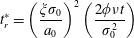 $$\begin{eqnarray}\displaystyle & \displaystyle t_{r}^{\ast }=\left(\frac{\unicode[STIX]{x1D709}\unicode[STIX]{x1D70E}_{0}}{a_{0}}\right)^{2}\left(\frac{2\unicode[STIX]{x1D719}\unicode[STIX]{x1D708}t}{\unicode[STIX]{x1D70E}_{0}^{2}}\right) & \displaystyle\end{eqnarray}$$
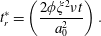 $$\begin{eqnarray}\displaystyle & \displaystyle t_{r}^{\ast }=\left(\frac{2\unicode[STIX]{x1D719}\unicode[STIX]{x1D709}^{2}\unicode[STIX]{x1D708}t}{a_{0}^{2}}\right). & \displaystyle\end{eqnarray}$$
Thus, for different sized non-buoyant vortex rings with geometrical similarity (
 $\unicode[STIX]{x1D6FE}_{0}=\text{const}.$
) propagating in the same fluid, a ring with smaller radius will experience higher relative expansion rates and vice versa. Considering this, the parameter
 $\unicode[STIX]{x1D6FE}_{0}=(\unicode[STIX]{x1D709}\unicode[STIX]{x1D70E}_{0}/a_{0})=(R_{0}/a_{0})$
emerges as providing a much more comprehensive physical understanding than a mere geometrical ratio. From (2.24) and (5.26), it can be interpreted as
 $$\begin{eqnarray}\frac{1}{\unicode[STIX]{x1D6FE}_{0}^{2}}=\frac{a_{0}^{2}}{R_{0}^{2}}=\frac{\text{viscous vorticity diffusion time scale}}{\text{ring expansion time scale}}.\end{eqnarray}$$
Further, it can be inferred from (5.14) that the rate of variation of the ring diameter is proportional to the rate of viscous dissipation, i.e. the rate of increase of the core size.
The above two equations (5.14) and (5.24) provide greater insights into the evolution of vortex rings. We see that, for thin rings, at
 $\unicode[STIX]{x1D6FE}_{0}\ll 1$
, the rate of radial expansion is significantly lower than the rate of viscous dissipation. This precisely means that
 $a^{\ast }$
will remain close to unity such that the vortex spacing
 $a$
will be invariant in time. If we use this constant-
 $a$
criteria in (1.5), we arrive at an expression for the propagation velocity which scales with
 $t^{-1}$
, which perfectly satisfies the short-time evolution equations.
As a thin-core vortex evolves in time, its core radius
 $R$
will expand continuously. This will also lead to a corresponding increase in the radial expansion velocity
 $V_{r}$
according to (5.14). As this process continues, the radial expansion of the ring will start to influence its translational velocity. At sufficiently large times, when the second term in (5.24) dominates over the third term,
 $a^{\ast }$
becomes proportional to
 $t^{1/2}$
. Thus, the vortex velocity profile migrates from
 $t^{-1}$
at short times to
 $t^{-3/2}$
at longer durations.
The above analysis can be utilized to further understand the impulse variation of vortex rings. The impulse of a self-propagating vortex ring is given by
 $$\begin{eqnarray}\displaystyle & \displaystyle I=\unicode[STIX]{x1D6FC}\unicode[STIX]{x1D6E4}a^{2}=\unicode[STIX]{x1D6FC}\unicode[STIX]{x1D6E4}_{0}\unicode[STIX]{x1D70E}_{0}\left(\frac{a^{2}}{\unicode[STIX]{x1D70E}^{2}}\right) & \displaystyle\end{eqnarray}$$
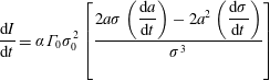 $$\begin{eqnarray}\displaystyle & \displaystyle \frac{\text{d}I}{\text{d}t}=\unicode[STIX]{x1D6FC}\unicode[STIX]{x1D6E4}_{0}\unicode[STIX]{x1D70E}_{0}^{2}\left[\frac{2a\unicode[STIX]{x1D70E}\displaystyle \left(\frac{\text{d}a}{\text{d}t}\right)-2a^{2}\left(\frac{\text{d}\unicode[STIX]{x1D70E}}{\text{d}t}\right)}{\unicode[STIX]{x1D70E}^{3}}\right] & \displaystyle\end{eqnarray}$$
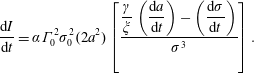 $$\begin{eqnarray}\displaystyle & \displaystyle \frac{\text{d}I}{\text{d}t}=\unicode[STIX]{x1D6FC}\unicode[STIX]{x1D6E4}_{0}^{2}\unicode[STIX]{x1D70E}_{0}^{2}(2a^{2})\left[\frac{\displaystyle \frac{\unicode[STIX]{x1D6FE}}{\unicode[STIX]{x1D709}}\left(\frac{\text{d}a}{\text{d}t}\right)-\left(\frac{\text{d}\unicode[STIX]{x1D70E}}{\text{d}t}\right)}{\unicode[STIX]{x1D70E}^{3}}\right]. & \displaystyle\end{eqnarray}$$
For
 $0<R/a\ll 1$
, when
 $(\text{d}a/\text{d}t)\ll (\text{d}\unicode[STIX]{x1D70E}/\text{d}t)$
, from the above equation, we hypothesize that the impulse of vortex rings should continuously decrease. For small times, when vortex spacing remains constant, the impulse should decrease continuously in the form
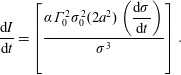 $$\begin{eqnarray}\frac{\text{d}I}{\text{d}t}=\left[\frac{\unicode[STIX]{x1D6FC}\unicode[STIX]{x1D6E4}_{0}^{2}\unicode[STIX]{x1D70E}_{0}^{2}(2a^{2})\displaystyle \left(\frac{\text{d}\unicode[STIX]{x1D70E}}{\text{d}t}\right)}{\unicode[STIX]{x1D70E}^{3}}\right].\end{eqnarray}$$
This loss of impulse was also reported by Maxworthy (Reference Maxworthy1972). He ascribed this loss to vorticity rejection to the wake. From (5.30), we also propose that this rate of impulse loss should vanish as time progresses, due to the balance between viscous dissipation and ring expansion. This precisely explains the mathematical form of the equations put forward for thick vortex rings, which are fundamentally built on the assumption of impulse conservation.
This explains the dynamics of non-buoyant vortex rings in the early- and moderate-time regimes when the vortex undergoes constant mass entrainment. In reality, vortex rings constantly undergo short- and long-wavelength instabilities due to strain induced on the cores as a result of convection motion (Tsai & Widnall Reference Tsai and Widnall1976; Jacquin et al.
Reference Jacquin, Fabre, Sipp, Theofilis and Vollmers2003). As the vorticity distribution spreads out, increasing its aspect ratio, or
 $\unicode[STIX]{x1D6FE}$
, short-wave instabilities increase exponentially, giving rise to secondary structures which lead to rapid vorticity decay, fluid detrainment and a transition to turbulence.
During this long-time regime, when vortex rings undergo net mass detrainment, the above theory predicts the shrinkage of vortex rings, as explained before. This phenomenon has also been observed and reported in many experimental and numerical studies (Hill Reference Hill1975; Nomura et al. Reference Nomura, Tsutsui, Mahoney and Rottman2006). Flow visualization pictures (figure 7) obtained for one of our experimental cases clearly shows this behaviour.
Equations (5.14) and (5.24) explain in detail the complex mechanism governing ring expansion. However, considering their complexity, these equations are not considered while deriving equations (2.34) to (2.35). We believe that such an attempt would make the solutions mathematically complex and visually unappealing, which would undermine the aim of this study. None the less, for considerably thick vortices where
 $\unicode[STIX]{x1D6FE}_{0}\rightarrow 1$
and the impulse remains roughly constant, we see that the equations stated in § 2 provide a good approximation for the observed phenomenon.
This novel approach thus provides a unification of the early and late regimes of vortex lifetime, and many previously observed anomalous phenomena can be qualitatively and mathematically explained.
5.3 Testing the fit of theory
The equations derived in § 2 show a gradual deviation from the experimental values for larger times. To understand this aspect quantitatively, we have performed a test of the fit for our primary variable
 $\unicode[STIX]{x1D714}_{max}$
. The entire dataset is divided into two parts, the training set and the cross-validation set, roughly in the ratio 60 : 40. Details about this approach are given in appendix B. Mean training set and cross-validation set errors for the experimental case C2-60 are plotted for an increasing number of dataset points (figure 18). Graphs for the other cases also show a similar trend.
Mean dataset errors: (a) training set, (b) cross-validation set.
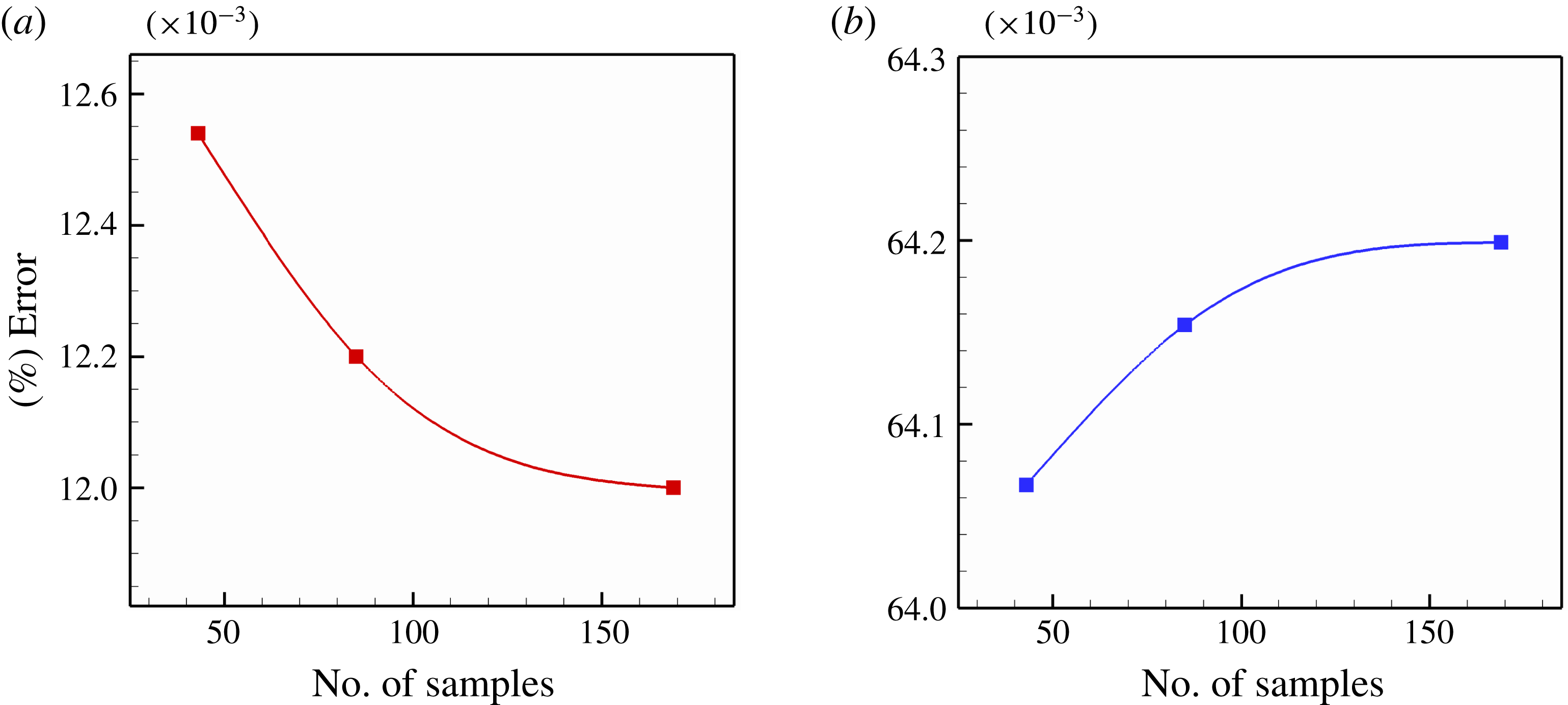
Errors in the cross-validation set are relatively higher than in the training set. This difference increases with an increase in the number of dataset points. In data-analysis terms, this condition is known as high variance. Such behaviour signifies underfitting, and indicates the need for higher-order terms in order to explain the observed phenomenon.
5.4 Comments on the value of
$\unicode[STIX]{x1D719}$

The equations derived in § 2 have been acquired considering
 $\unicode[STIX]{x1D719}$
to remain constant throughout the evolution phase. However, from table 2, we see that the value of
 $\unicode[STIX]{x1D719}$
that best describes the motion varies with Reynolds number. Hence, in reality, as the vortex slows down during propagation and
 $Re$
changes continuously, the value of
 $\unicode[STIX]{x1D719}$
also changes accordingly:
 $$\begin{eqnarray}\unicode[STIX]{x1D719}=f(\unicode[STIX]{x1D714}_{max},\unicode[STIX]{x1D70E},\unicode[STIX]{x1D708}).\end{eqnarray}$$
Realizing this time-varying nature of
 $\unicode[STIX]{x1D719}$
, one could account for the observed higher-order behaviour, and thus provide a better fit.
6 Conclusion
This study provides enhanced physical insights into the mechanism governing vortex evolution using a novel and effective mathematical framework. The ideas presented here are simple enough to form a part of an undergraduate textbook, but at the same time, it provides elegant and profound physical understanding of many observed, but so far unexplained phenomena. Approach used in this study carefully scrutinize and signify the role played by various vortex parameters, and many important inferences can be drawn.
Firstly, it shows that vorticity evolution is primarily governed by viscous diffusion, with negligible influence of vortex inertia. Also, for Reynolds numbers ranging between 100 and 10000, the vortex core can be approximated to be circular without much loss of accuracy. Theoretical expressions derived in § 2 effectively explain the temporal variation in peak vorticity and core size as observed in experiments. This study also challenges the accepted theories of vorticity decay and suggests an alternate understanding into this subject. It provides a quantitative measure of circulation reduction which was hitherto unaddressed.
The transitional theory described in § 5.2 sheds light on the precise role of the Reynolds number and slenderness ratio in the vortex evolution mechanism. The vortex Reynolds number governs the rate of viscous dissipation of vorticity, which results in core expansion. This increase in core size is, however, independent of the slenderness ratio (
 $R/a$
). On the other hand, the slenderness ratio plays a major role in ring expansion, with minimal influence of the Reynolds number. This addresses the long-standing confusion.
To be precise, the absolute extent of core expansion (
 $\unicode[STIX]{x1D70E}$
) and ring expansion (
 $a$
) are governed independently by the following two time scales
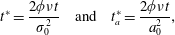 $$\begin{eqnarray}t^{\ast }=\frac{2\unicode[STIX]{x1D719}\unicode[STIX]{x1D708}t}{\unicode[STIX]{x1D70E}_{0}^{2}}\quad \text{and}\quad t_{a}^{\ast }=\frac{2\unicode[STIX]{x1D719}\unicode[STIX]{x1D708}t}{a_{0}^{2}},\end{eqnarray}$$
whereas
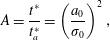 $$\begin{eqnarray}A=\frac{t^{\ast }}{t_{a}^{\ast }}=\left(\frac{a_{0}}{\unicode[STIX]{x1D70E}_{0}}\right)^{2},\end{eqnarray}$$
which is a function of the slenderness ratio, signifies only the relative expansion rates. Moreover, this study concludes that vortex ring evolution can be classified into three phases. For
 $A>100$
, ring expansion is negligible and short-time behaviour can be observed. This can be termed as the ‘nascent’ stage, where the velocity follows (1.2). On the other hand, for
 $A<10$
, the vorticity diffusion rate is comparable to the ring expansion. This is the ‘matured’ stage, when velocity follows ‘
 $t^{-3/2}$
’ law. Between these two extremes, no single time scale governs the vortex ring evolution. Thus, this theory forms a bridge between the existing asymptotic theories, and the above time scales rationalize many anomalous observations reported in the literature.
In addition to the above, § 2 displays a new approach for studying self-similarity problems. Though we have addressed vorticity diffusion only, the same approach can be used for studying other phenomena as well.
Finally, some phenomena such as elliptical core, short- and long-wavelength instabilities have also been observed in the experiments. These are, however, not discussed due to their complex nature and miniscule advantage, over and above the present, for understanding the underlying physics. Nevertheless, our theory offers a comprehensive understanding of many of the observed phenomenon, and promises important applications.
This study can be utilized for understanding the evolution of aircraft wing tip vortices and could help in determining better air traffic standards. The methods used in § 2 can also be extended further to analyse equations with momentum and energy source and sink terms, which physically describe the mechanisms governing tornadoes and hurricanes, for example. An accurate understanding of the time-varying nature of vortex size and strength because of this attempt, could prove instrumental for gauging weather forecasts, leading to better disaster management with a direct impact on human life.
Acknowledgements
We gratefully acknowledge funding and support received from Solar Energy Research Institute for India and the United States (SERIIUS) and DST-SERI-Project no. DST/TMC/SERI/FR/136.
Supplementary material
Supplementary material is available at https://doi.org/10.1017/jfm.2017.815.
Appendix A. Gradient inversion method for finding the best-fit curve
This is an in-house technique used for finding the best-fit parameter (
 $\unicode[STIX]{x1D719}$
) in § 4 based on experimentally obtained values. We are familiar with the optimization of a continuous function where local stagnation points are obtained when the first derivative of the objective function (
 $Z$
) vanishes i.e.
 $$\begin{eqnarray}\displaystyle & \displaystyle \frac{\text{d}Z(x)}{\text{d}x}=0 & \displaystyle\end{eqnarray}$$
 $$\begin{eqnarray}\displaystyle & \displaystyle z=\mathop{\sum }_{i=1}^{n}|Y_{x_{i}}-f(x_{i})|, & \displaystyle\end{eqnarray}$$
where
 $n$
is the total sample size;
 $Y(x_{i})$
is the experimentally obtained value of
 $Y$
at
 $x=x_{i}$
and
 $f(x)$
is our analytical equation. However, the above-mentioned calculus approach of optimization is suitable only for continuous functions and is ineffective for discrete datasets where the derivative (A 1) may always carry a non-zero value. Other statistical techniques, such as stochastic and deterministic gradient descent, are also of limited use since their accuracy depends upon a predetermined minimum acceptable error value, which is difficult to comprehend for varying experimental conditions. Thus, a novel and robust method of local optimization is developed to satisfy our requirements, which is given below.
1. Start
2. Initialize parameter
 $\unicode[STIX]{x1D6FD},k,\text{d}\unicode[STIX]{x1D6FD}$
3. Start-loop: calculate sum
 $Z$
4.
 $\unicode[STIX]{x1D6FD}=\unicode[STIX]{x1D6FD}+k(\text{d}\unicode[STIX]{x1D6FD})$
5. If
 $Z_{\unicode[STIX]{x1D6FD}}>Z_{\unicode[STIX]{x1D6FD}+k(\text{d}\unicode[STIX]{x1D6FD})},k=1$
else
 $k=(-1)$
6. If
 $k$
changes sign a second time: break
7. Else: Go to Start-loop
8. Return
 $\unicode[STIX]{x1D6FD}$
9. End
The above algorithm was coded in MATLAB. Under this method, local minimization of
 $Z$
is reported when the gradient undergoes sign reversal for the second time. Using a constant and user-defined value of
 $\text{d}\unicode[STIX]{x1D6FD}$
, this program helps us to gain the desired resolution on the independent variable value (
 $\unicode[STIX]{x1D6FD}$
here), thus overcoming the shortcomings of the other methods.
Appendix B. Test of fit
In order to validate our theoretical expressions, we have conducted a test-of-fit analysis using our experimental data and the best-fit equations. For this attempt, the entire dataset of primary variable (vorticity here) is divided into two separate sets: ‘training set’ and ‘cross-validation set’, in the ratio
 $60:40$
, respectively (figure 19). The theoretical expression is fitted onto the base set using the technique described in appendix A.
Schematic explaining the process of testing the hypothesis.
The obtained best fit equation is then tested to check its validity on the cross-validation set. A measure of fit of an equation is quantified by the mean absolute error, given by
 $$\begin{eqnarray}E=\frac{1}{n}\mathop{\sum }_{i=1}^{n}|Y_{i}-f(x_{i})|.\end{eqnarray}$$
The above error is calculated on both the base set and cross-validation set for different sample sizes of 100 %, 50 % and 25 %. Error values for different cropped sets are then compiled with an increasing number of sample points, as shown in figure 17.
For a good fit, the individual errors in ‘base set’ will continue to decrease and flatten as the number of sample points is increased. However, when these error values are significantly lower than that in the CV set, it indicates that the analytical equation satisfies the observed behaviour only for the short period and deviates at later stages. Moreover, when the CV set errors increase nonlinearly with an increase in the number of sample points, it bolsters the understanding that higher-order behaviour is prevalent which can only be captured by incorporating higher orders of the variables. This condition is known as ‘variance’.