1. Introduction
Gas flow in porous media in the presence of Knudsen effects, more particularly in the slip regime, has been the subject of considerable attention since the pioneering empirical work of Klinkenberg (Reference Klinkenberg1941). Whenever the Knudsen number,  $\textit {Kn}$, of the flow, which may be defined as the ratio of the mean free path of the gas molecules to the pore-size, is not exceedingly small compared with unity, the no-slip boundary condition at the pore solid–fluid interfaces is inappropriate. For values of
 $\textit {Kn}$ up to approximately 0.1, the pore-scale flow problem can be stated in the classical continuum mechanics framework. It consists of the Navier–Stokes equations for momentum transport along with a Navier (first-order) slip boundary condition (Navier Reference Navier1822) at the solid–fluid interfaces, which reflects interactions between gas particles and the porous solid skeleton. At the macroscopic scale, this results in a modified Darcy's law, in which the permeability is no longer intrinsic but
 $\textit {Kn}$-dependent. While the popular one-dimensional Darcy–Klinkenberg form of the macroscopic momentum equation has been widely employed for homogeneous (Wu, Pruess & Persoff Reference Wu, Pruess and Persoff1998; Hayek Reference Hayek2015) and heterogeneous (Chastanet, Royer & Auriault Reference Chastanet, Royer and Auriault2004) porous media, a detailed physically sound and complete (three-dimensional) macroscopic model was recently derived, which considers slightly compressible, but steady, creeping flow conditions for the gas (Lasseux et al. Reference Lasseux, Valdés-Parada, Ochoa-Tapia and Goyeau2014; Lasseux, Valdés-Parada & Porter Reference Lasseux, Valdés-Parada and Porter2016). Homogenization was also used to upscale this problem with the classical Navier-type slip condition (Allaire Reference Allaire1991) as well as with a more complex slip boundary condition (Cioranescu, Donato & Ene Reference Cioranescu, Donato and Ene1996).
In many situations, however, the forcing may not be steady and, even if the flow remains in the creeping regime, the temporal acceleration term can be of importance in the momentum balance at the pore-scale. The question then arises about the appropriate macroscopic model applicable to an equivalent homogeneous medium. To the best of our knowledge, the derivation of a macroscale model for this situation has not yet been adequately addressed in the literature.
For incompressible flows in the absence of Knudsen effects, a common practice has been to employ a heuristic macroscopic model. This consists in empirically using an analogue of the unsteady Stokes (or Navier–Stokes) equations in which the pore-scale velocity is replaced by the superficial average (or filtration) velocity, and the forcing by the Darcy term corresponding to the average drag on the solid matrix of the porous medium (Polubarinova-Kochina Reference Polubarinova-Kochina1962; Nield & Bejan Reference Nield and Bejan2013; Das, Mukherjee & Muralidhar Reference Das, Mukherjee and Muralidhar2018). Such a model has been employed in several different situations, such as flows in fluid-porous media systems (Breugem, Boersma & Uittenbogaard Reference Breugem, Boersma and Uittenbogaard2006; Jin & Kuznetsov Reference Jin and Kuznetsov2017) and their stability analysis (Hill & Straughan Reference Hill and Straughan2008; Samanta Reference Samanta2020), fluid motion in a porous medium with slip at the macroscopic boundaries of the domain (Haddad, Al-Nimr & Sari Reference Haddad, Al-Nimr and Sari2007; Qayyum et al. Reference Qayyum, Khan, Rahim and Ullah2015), and magnetohydrodynamic (MHD) flows (Ullah, Khan & Shafie Reference Ullah, Khan and Shafie2017; Nandal, Kumari & Rathee Reference Nandal, Kumari and Rathee2019), among others. However, as suggested by Auriault (Reference Auriault1980) and Allaire (Reference Allaire1992), and further elaborated by Lasseux, Valdés-Parada & Bellet (Reference Lasseux, Valdés-Parada and Bellet2019) and Bottaro (Reference Bottaro2019) in a more general framework including inertial effects, the macroscopic model obtained by formal upscaling of the pore-scale equations, and validated by several numerical examples, does not correspond, in general, to the heuristic form, which relies on a separation of time scales between the pore-scale and the macroscale.
Straightforward extension of the heuristic macroscopic momentum equation to the case where a slip condition applies at the solid–fluid interfaces at the pore-scale may certainly be appealing. An attempt to obtain such a model, starting from the Boltzmann equations to account for the gas–solid interactions at the pore level, was proposed by Pavan & Oxarango (Reference Pavan and Oxarango2007) (see their resulting equation (27)). However, no validation of this model was explored. In light of previous investigations carried out in the absence of slip, a more thorough analysis of the unsteady form of the macroscopic model when slip effects are present appears to be of major interest and motivates the present work.
With this purpose in mind, the article is organized as follows. In § 2, the pore-scale initial-boundary-value problem for unsteady, creeping, slightly compressible and isothermal flow in a homogeneous porous material is presented. The equation of state is formulated in a general framework, without assuming a special form a priori. The slip boundary condition at this scale is a Navier-type condition. Although written in the context of gas flow involving Knudsen effect, it may also be regarded as an effective one, resulting from pre-upscaling of a no-slip condition over rough surfaces (see for instance Pasquier, Quintard & Davit Reference Pasquier, Quintard and Davit2017). In § 3, this problem is upscaled using a modified version of the volume averaging method (Whitaker Reference Whitaker1999) combined with the associated fundamental problem for the velocity Green's function pair (Choi & Dong Reference Choi and Dong2021) and Green's formula (derived in Appendix A), which results in an approach that is equivalent to the adjoint homogenization method (Bottaro Reference Bottaro2019), briefly reported in Appendix B. The two effective parameters involved in the resulting average model operating at the macroscopic level (namely an apparent dynamic permeability tensor and a vector accounting for the memory effects of the initial condition) are obtained from the solution of a single and novel closure problem that is independent of the initial conditions and forcings. Analysis of the symmetry properties of the apparent dynamic permeability tensor is provided in Appendix C. The proper expected convergence of the unsteady average model towards its steady version (Lasseux et al. Reference Lasseux, Valdés-Parada and Porter2016), when steady conditions are met, is detailed in Appendix D. The whole procedure leads to a closed set of macroscopic equations, which include mass and momentum balance, as well as a generic equation of state, the closure of which is detailed in Appendix E. Section 4 is dedicated to a validation of the averaged model that is carried out through comparisons with direct numerical simulations (DNS) of the pore-scale equations for a model problem. A further comparison is also provided with the predictions of the heuristic model. Finally, conclusions are drawn in § 5.
2. Pore-scale model
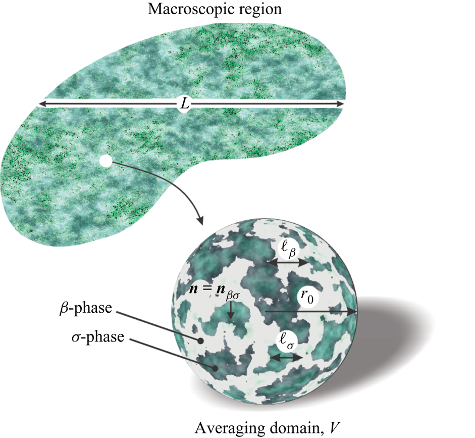
Consider the single-phase flow of a Newtonian fluid in a rigid and homogeneous porous medium, such as the one sketched in figure 1 in which  $\beta$ and
 $\sigma$ respectively denote the fluid and solid phases. The governing equation for mass transport at the pore-scale within a periodic unit cell for this physical configuration is
 \begin{equation} \frac{\partial \rho }{\partial t} +\boldsymbol{\nabla} \boldsymbol{\cdot} (\rho \boldsymbol{v}) =0, \quad \text{in the}\ \beta \text{-phase}. \end{equation}
Here  $\boldsymbol {v}$ and
 $\rho$ are the fluid velocity and density, respectively, and
 $t$ is time. For momentum transport, the creeping flow regime is assumed, i.e. the Reynolds number, defined as
 $Re=\rho _r v \ell _{\beta }/\mu$, is small compared with unity. Here,
 $\rho _r$,
 $\ell _{\beta }$ and
 $v$ are respectively a reference density, the characteristic pore size and velocity magnitude. As a result, the convective acceleration term is neglected with respect to the viscous term, which leads to the unsteady Stokes equation:
 \begin{equation} \frac{\partial\left(\rho\boldsymbol{v}\right)}{\partial t} ={-}\boldsymbol{\nabla} p +\mu \boldsymbol{\nabla}\boldsymbol{\cdot} \left( \boldsymbol{\nabla}\boldsymbol{v} +\boldsymbol{\nabla} \boldsymbol{v}^T\right) +\left( \eta -\frac{2}{3}\mu \right)\boldsymbol{\nabla} (\boldsymbol{\nabla}\boldsymbol{\cdot} \boldsymbol{v}), \quad \text{in the}\ \beta \text{-phase}. \end{equation}
In this momentum balance equation,  $p$ represents the pore-scale pressure, whereas
 $\mu$ and
 $\eta$ are respectively the shear and bulk viscosities, which are assumed constant in the rest of this work.
Sketch of a rigid porous medium system of characteristic length  $L$ saturated with a single fluid phase and averaging domain of characteristic size
 $r_0$. The characteristic lengths of the solid and fluid phases are
 $\ell _\sigma$ and
 $\ell _\beta$, respectively.

Equations (2.1a) and (2.1b) are completed with an equation of state relating the fluid density to pressure and temperature. Assuming isothermal flow, this relationship can be written as a functional dependence of  $\rho$ upon the pressure
 $p$. The developments that follow do not require specifying a particular form of this function; hence it suffices here to write
 \begin{equation} \rho = F(p). \end{equation}
At the solid–fluid interface in the entire macroscopic system,  $\mathscr {A}_{\beta \sigma M}$, no mass flux is assumed and the following first-order slip boundary condition is imposed (Navier Reference Navier1822; Lockerby et al. Reference Lockerby, Reese, Emerson and Barber2004; Lauga, Brenner & Stone Reference Lauga, Brenner and Stone2007):
 \begin{equation} \boldsymbol{v} ={-}\xi \lambda ({\boldsymbol{\mathsf{I}}}-\boldsymbol{n}\boldsymbol{n})\boldsymbol{\cdot} \left[ \boldsymbol{n}\boldsymbol{\cdot} \left(\boldsymbol{\nabla} \boldsymbol{v}+\boldsymbol{\nabla}\boldsymbol{v}^T \right) \right], \quad \text{at}\ \mathscr{A}_{\beta\sigma M}. \end{equation}
In this relationship,  $\xi = (2-\sigma _v)/\sigma _v$, where
 $\sigma _v$ is the tangential momentum accommodation coefficient. In practice,
 $\xi =\boldsymbol {O}(1)$ with values ranging between 1.3 and 1.7 (see for e.g. Perrier et al. Reference Perrier, Graur, Ewart and Méolans2011). In addition,
 $\lambda$ is the mean-free path of the fluid molecules given by (Cowling Reference Cowling1950):
 \begin{equation} \lambda = \frac{M}{\sqrt{2} \,{\rm \pi} \,\mathcal{N}_A \,\rho \, d_m^2}, \end{equation}
where  $M$ is the molar mass of the gas,
 $\mathcal {N}_A$ the Avogadro number and
 $d_m$ the particle diameter. Moreover, in the slip boundary condition,
 ${\boldsymbol{\mathsf{I}}}$ is the identity tensor and
 $\boldsymbol {n}$ denotes the unit normal vector to
 $\mathscr {A}_{\beta \sigma M}$, directed from the fluid-phase to the solid-phase (see figure 1). It should be noted that the formalism employed here refers to slip associated with Knudsen effects. However, this type of boundary condition may also be envisaged in a more general framework as the effective one resulting from an upscaling process, from the roughness scale to the pore-scale, of the no-slip boundary condition at rough pore–solid inclusions interfaces, as proposed by Pasquier et al. (Reference Pasquier, Quintard and Davit2017).
A complete problem statement requires accounting for the boundary conditions applicable at the inlets and outlets of the macroscopic system. However, this information is not necessary for the developments that follow, which are restricted to a region sufficiently far from these boundaries. Finally, the initial conditions for the pore-scale velocity and density are given by
 \begin{equation} \text{when } t=0, \quad \boldsymbol{v}=\boldsymbol{v}_0(\boldsymbol{r}), \quad \rho = \rho_0 (\boldsymbol{r}). \end{equation}
Here  $\boldsymbol {v}_0$ and
 $\rho _0$ are known functions of position. Note that the choice is made to specify the density at
 $t=0$. An equivalent statement could have been made in terms of the initial value of the pressure.
The purpose of this work is to derive the average flow model, i.e. the average mass and momentum balances as well as the equation of state applicable in the porous medium bulk (i.e. far from macroscopic boundaries). To this end, double scale periodic homogenization could be considered as proposed, for instance, by Mikelić (Reference Mikelić1994) or Khuzhayorov, Auriault & Royer (Reference Khuzhayorov, Auriault and Royer2000). In the present work, the volume averaging method (Whitaker Reference Whitaker1999) is employed to derive the macroscopic mass conservation equation, while the macroscopic momentum balance equation and the equation of state are obtained by making use of the fundamental problem for the velocity Green's function pair and Green's formula, an approach similar to the adjoint homogenization method proposed by Bottaro (Reference Bottaro2019).
3. Derivation of the upscaled model
3.1. Preliminaries
Let the derivations begin by defining an averaging domain,  $\mathscr {V}$, of volume
 $V$ which contains portions of the fluid and solid phases (see figure 1). For this domain to be representative, its characteristic size,
 $r_0$, must be much larger than the largest of the characteristic sizes at the pore-scale (i.e.
 $\ell _p=\max (\ell _\beta ,\ell _\sigma )$) and, at the same time, much smaller than the smallest length scale associated with the macroscale (
 $L$). This can be expressed in the following form (Bear Reference Bear2018):
 \begin{equation} \ell_p\ll r_0 \ll L. \end{equation}
In terms of this averaging domain, it is possible to define the superficial and intrinsic averaging operators that apply to any piecewise smooth function,  $\psi$, defined everywhere in the fluid phase as follows:
 \begin{align} \langle \psi\rangle = \frac{1}{V}\int_{\mathscr{V}_\beta} \psi\,\textrm{d}V, \end{align}
 \begin{align} \langle \psi\rangle^\beta = \frac{1}{V_\beta}\int_{\mathscr{V}_\beta} \psi\,\textrm{d}V, \end{align}
where  $\mathscr {V}_\beta$ (of volume
 $V_\beta$) represents the space occupied by the fluid phase within the averaging domain. These two averaging operators are related by
 \begin{equation} \langle \psi\rangle = \varepsilon\langle \psi \rangle^\beta, \end{equation}
where  $\varepsilon = V_\beta /V$ denotes the fluid volume fraction within the averaging domain, i.e. the porosity, which is assumed to be constant in both space and time in the rest of this work. Furthermore, in the volume averaging method, it is often required to interchange the operations of spatial integration and differentiation. This is achieved by means of the spatial averaging theorem (or Leibniz rule), which, for the gradient operator, can be expressed as (see e.g. Howes & Whitaker Reference Howes and Whitaker1985)
 \begin{equation} \langle \boldsymbol{\nabla} \psi \rangle = \boldsymbol{\nabla} \langle \psi\rangle +\frac{1}{V}\int_{\mathscr{A}_{\beta\sigma}} \boldsymbol{n}\, \psi\,\textrm{d}A. \end{equation}
A similar form applies to the divergence operator.
To carry out the developments that follow, it is convenient to introduce the spatial decomposition given by (see e.g. Gray Reference Gray1975)
 \begin{equation} \psi = \langle \psi\rangle^\beta +\tilde{\psi}. \end{equation}
Here  $\tilde {\psi }$ represents the spatial deviations of
 $\psi$ with respect to its intrinsic average. In essence, the decomposition operates a decoupling between the fast varying part,
 $\tilde {\psi }$ of
 $\psi$, from its slow varying part,
 $\langle \psi \rangle ^\beta$, as in the homogenization method (Auriault, Boutin & Geindreau Reference Auriault, Boutin and Geindreau2009). With this in mind, it is important to note that while
 $\psi$ is considered at any position
 $\boldsymbol {r}$ within
 $\mathscr {V}_\beta$,
 $\langle \psi \rangle$ and
 $\langle \psi \rangle ^\beta$ are dependent on
 $\boldsymbol {x}$, which locates the centroid of the averaging domain. As a corollary, it is pertinent to note that when the averaging domain is representative (i.e. when the inequality given in (3.1) is met), average fields can be assumed to be constant within
 $\mathscr {V}_\beta$ so that the fields of the spatial deviations are bounded by the following average constraint:
 \begin{equation} \langle \tilde{\psi} \rangle^\beta =0. \end{equation}
In the remainder of this work, the flow is assumed to be slightly compressible. This hypothesis means that the density fluctuations  $\tilde {\rho }$ satisfy the constraint,
 \begin{equation} \tilde{\rho} \ll \langle \rho \rangle^\beta, \end{equation}
everywhere within the averaging domain, at any time. The supporting constraints and assumptions justifying this hypothesis are available from the work of Lasseux et al. (Reference Lasseux, Valdés-Parada, Ochoa-Tapia and Goyeau2014). As a result, the following approximation is employed:
 \begin{equation} \rho \simeq \langle \rho \rangle^\beta. \end{equation}
3.2. Macroscopic mass equation
Due to the slightly compressible flow assumption expressed in (3.8), the pore-scale mass balance equation (2.1a) may be rewritten within the averaging domain as
 \begin{equation} \frac{\partial \langle \rho \rangle ^\beta }{\partial t} +\boldsymbol{\nabla}\boldsymbol{\cdot} (\langle \rho \rangle^\beta \boldsymbol{v}) =0, \quad \text{in the}\ \beta\text{-phase.} \end{equation}
Applying the superficial averaging operator to this equation, together with the spatial averaging theorem, and using the fact that  $\mathscr {V}_\beta$ is constant in time, yields
 \begin{equation} \varepsilon \frac{\partial \langle \rho \rangle^\beta}{\partial t} + \boldsymbol{\nabla} \boldsymbol{\cdot} \left( \langle \rho\rangle^\beta \langle \boldsymbol{v} \rangle \right) + \frac{\langle \rho \rangle ^\beta}{V}\int_{\mathscr{A}_{\beta\sigma}} \boldsymbol{n}\boldsymbol{\cdot} \boldsymbol{v}\,\textrm{d}A =0. \end{equation}
Since the slip velocity at  $\mathscr {A}_{\beta \sigma }$ is, by definition, tangential to the surface in accordance with the fact that no mass is exchanged between the fluid and the solid phases, the macroscopic mass balance equation takes the following final form:
 \begin{equation} \varepsilon \frac{\partial \langle \rho \rangle^\beta}{\partial t} + \boldsymbol{\nabla}\boldsymbol{\cdot} \left( \langle \rho\rangle^\beta \langle \boldsymbol{v} \rangle \right) =0. \end{equation}
3.3. Macroscopic momentum equation
In order to derive the macroscopic balance equation for momentum transport, it is convenient to assume that the porous medium geometry contained in the averaging domain can be represented by a periodic array of unit cells. The pore-scale equations presented above are now considered in this unit cell. For the developments that follow, it is useful to define the mass flux  $\boldsymbol {q}$ as
 \begin{equation} \boldsymbol{q}=\langle \rho \rangle ^\beta \boldsymbol{v}; \end{equation}
which allows writing the pore-scale mass conservation equation (3.9a) as
 \begin{equation} \frac{\partial \langle \rho \rangle ^\beta }{\partial t} +\boldsymbol{\nabla}\boldsymbol{\cdot} \boldsymbol{q} =0 , \quad \text{in the}\ \beta\text{-phase.} \end{equation}
Directing attention to the pore-scale momentum transport equation and introducing the spatial decomposition of the pressure, while keeping in mind that  $\langle \rho \rangle ^\beta$ can be considered as a constant within the unit cell, allows expression of the momentum balance in the following form:
 \begin{equation} \frac{1}{\mu}\frac{\partial \boldsymbol{q}}{\partial t} ={-} \frac{1}{\mu} \boldsymbol{\nabla} \tilde{p} + \frac{1}{\langle \rho \rangle ^\beta}\boldsymbol{\nabla}\boldsymbol{\cdot} \left( \boldsymbol{\nabla}\boldsymbol{q}+\boldsymbol{\nabla}\boldsymbol{q}^T\right) +\frac{\kappa}{\langle \rho \rangle ^\beta}\nabla (\boldsymbol{\nabla}\boldsymbol{\cdot} \boldsymbol{q}) -\frac{1}{\mu} \boldsymbol{\nabla} \langle p\rangle^\beta, \quad \text{in the}\ \beta\text{-phase.} \end{equation}
with  $\kappa =\eta /\mu -2/3$ a dimensionless modified viscosity coefficient.
In addition, the boundary condition at the solid–fluid interfaces contained in the unit cell,  $\mathscr {A}_{\beta \sigma }$, can be rewritten, after replacing
 $\lambda$ by
 $\bar {\lambda }$, as
 \begin{equation} \boldsymbol{q} ={-}\xi \bar{\lambda} ({\boldsymbol{\mathsf{I}}}-\boldsymbol{n}\boldsymbol{n})\boldsymbol{\cdot} \left[ \boldsymbol{n}\boldsymbol{\cdot} \left(\boldsymbol{\nabla} \boldsymbol{q}+\boldsymbol{\nabla}\boldsymbol{q}^T \right) \right], \quad \text{at}\ \mathscr{A}_{\beta\sigma}, \end{equation}
where  $\bar {\lambda }$ is defined in terms of
 $\langle \rho \rangle ^\beta$ using an approximation consistent with the slightly compressible assumption, as explained in detail by Lasseux et al. (Reference Lasseux, Valdés-Parada, Ochoa-Tapia and Goyeau2014), i.e.
 \begin{equation} \bar{\lambda} = \frac{M}{\sqrt{2} \,{\rm \pi}\, \mathcal{N}_A \langle \rho \rangle^\beta d_m^2}. \end{equation}
For the problem to be well posed, the average constraint given in (3.6) is applied to the pressure deviations,
 \begin{equation} \langle \tilde{p}\rangle^\beta =0. \end{equation}
The initial conditions for the velocity and density in the periodic unit cell follow from (2.1f), i.e.
 \begin{equation} \text{when } t=0, \quad \boldsymbol{q}= \boldsymbol{q}_0 \equiv \langle \rho_0 (\boldsymbol{r})\rangle ^\beta\boldsymbol{v}_0(\boldsymbol{r}), \quad \langle \rho \rangle ^\beta= \langle \rho_0 (\boldsymbol{r})\rangle ^\beta. \end{equation}
Finally, within the porous medium bulk, it is reasonable to assume that the pressure deviations and velocity are periodic at the inlets and outlets of the unit cell. Consequently, the following boundary conditions are imposed:
 \begin{equation} \psi(\boldsymbol{r}+\boldsymbol{l}_i)=\psi(\boldsymbol{r}), \quad i=1,2,3; \quad \psi = \boldsymbol{q}, \tilde{p}, \end{equation}
 $\boldsymbol {r}$ being a position vector locating any point at the boundaries of the unit cell within the fluid phase and
 $\boldsymbol {l}_i$ denoting the unit cell lattice vectors.
With the intention of deriving an upscaled momentum transport model, consider first the following fundamental problem for the velocity Green's function pair  $({\boldsymbol{\mathsf{G}}}_v,\boldsymbol {g}_p)$ given by (Choi & Dong Reference Choi and Dong2021)
 \begin{gather} \boldsymbol{\nabla} \boldsymbol{\cdot} {\boldsymbol{\mathsf{G}}}_v=\boldsymbol{0}, \quad \text{in the} \beta\text{-phase}, \end{gather}
 \begin{gather}-\frac{1}{\mu}\frac{\partial {\boldsymbol{\mathsf{G}}}_v}{\partial t} ={-}\boldsymbol{\nabla} \boldsymbol{g}_p+\frac{1}{\langle \rho \rangle ^\beta}\boldsymbol{\nabla}\boldsymbol{\cdot} \left( \boldsymbol{\nabla} {\boldsymbol{\mathsf{G}}}_v +\boldsymbol{\nabla} {\boldsymbol{\mathsf{G}}}_v^{{T}1}\right) , \quad \text{in the}\ \beta\text{-phase}, \end{gather}
 \begin{gather}{\boldsymbol{\mathsf{G}}}_v ={-}\xi \bar{\lambda}\left( {\boldsymbol{\mathsf{I}}}-\boldsymbol{n}\boldsymbol{n}\right) \boldsymbol{\cdot} \left[ \boldsymbol{n}\boldsymbol{\cdot} \left( \boldsymbol{\nabla} {\boldsymbol{\mathsf{G}}}_v+ \boldsymbol{\nabla} {\boldsymbol{\mathsf{G}}}_v^{{T}1}\right) \right], \quad \text{at }\mathscr{A}_{\beta\sigma}, \end{gather}
 \begin{gather}\langle \boldsymbol{g}_p\rangle^\beta =\boldsymbol{0}, \end{gather}
 \begin{gather}\text{when } t=t_f, \quad {\boldsymbol{\mathsf{G}}}_v=\frac{\mu}{\langle \rho \rangle ^\beta} \delta(\boldsymbol{r}-\boldsymbol{r}_0) {\boldsymbol{\mathsf{I}}}, \end{gather}
 \begin{gather}\psi(\boldsymbol{r}+\boldsymbol{l}_i)=\psi(\boldsymbol{r}), \quad i=1,2,3; \quad \psi = {\boldsymbol{\mathsf{G}}}_v, \boldsymbol{g}_p. \end{gather}
Here  ${{\boldsymbol{\mathsf{G}}}}_v\equiv {{\boldsymbol{\mathsf{G}}}}_v (\boldsymbol {r}, \boldsymbol {r}_0, t_f,t)$ and
 $\boldsymbol {g}_p\equiv \boldsymbol {g}_p (\boldsymbol {r}, \boldsymbol {r}_0, t_f,t)$ are functions that map the influence of a source located at
 $\boldsymbol {r}_0$ and
 $t_f$ onto the fluid velocity and the pressure deviations at
 $\boldsymbol {r}$ and
 $t$, respectively. In (3.12b), the superscript
 ${T}1$ denotes the transpose of a third-order tensor that permutes the two first indices, i.e.
 $(\boldsymbol {\nabla } {{\boldsymbol{\mathsf{G}}}}_v^{{T}1})_{ijk}=(\boldsymbol {\nabla } {{\boldsymbol{\mathsf{G}}}}_v)_{jik}$. In this problem,
 $\langle \rho \rangle ^\beta$ and
 $\bar {\lambda }$ are evaluated at
 $\boldsymbol {x}$ and
 $t$. Note that, although
 $\boldsymbol {\nabla }\boldsymbol {\cdot }(\boldsymbol {\nabla }{{\boldsymbol{\mathsf{G}}}}_v^{{T}1})=\boldsymbol {0}$ since
 ${{\boldsymbol{\mathsf{G}}}}_v$ is solenoidal, this term is maintained in (3.12b) for convenience. Nevertheless, the term
 $({\kappa }/{\langle \rho \rangle ^\beta } )\boldsymbol {\nabla } (\boldsymbol {\nabla }\boldsymbol {\cdot } {{\boldsymbol{\mathsf{G}}}}_v)$ was omitted because of this property on
 ${{\boldsymbol{\mathsf{G}}}}_v$. It should also be noted that
 ${{\boldsymbol{\mathsf{G}}}}_v$ is a symmetric tensor (Pozrikidis Reference Pozrikidis1992; Haberman Reference Haberman2012) and, as a result,
 $\boldsymbol {\nabla }\boldsymbol {g}_p$ is also symmetric.
Since the interest lies in the derivation of an expression for the average velocity, it is more convenient to proceed with the adjoint problem of the original physical one by carrying out an integration over  $\mathscr {V}_\beta (\boldsymbol {r}_0)$ of the above problem for the velocity Green's function pair. Denoting
 \begin{equation} {\boldsymbol{\mathsf{M}}} (\boldsymbol{r}, t_f, t) = \int_{\mathscr{V}_\beta (\boldsymbol{r}_0)} {\boldsymbol{\mathsf{G}}}_v(\boldsymbol{r}, \boldsymbol{r}_0, t_f, t)\,\textrm{d}V(\boldsymbol{r}_0) \end{equation}
and
 \begin{equation} \boldsymbol{m} (\boldsymbol{r}, t_f, t) = \int_{\mathscr{V}_\beta (\boldsymbol{r}_0)} {\boldsymbol{g}}_p(\boldsymbol{r}, \boldsymbol{r}_0, t_f, t)\,\textrm{d}V(\boldsymbol{r}_0), \end{equation}
the following problem is obtained:
 \begin{gather} \boldsymbol{\nabla} \boldsymbol{\cdot} {\boldsymbol{\mathsf{M}}}=\boldsymbol{0}, \quad \text{in the}\ \beta\text{-phase}, \end{gather}
 \begin{gather}-\frac{1}{\mu}\frac{\partial {\boldsymbol{\mathsf{M}}}}{\partial t} ={-}\boldsymbol{\nabla} \boldsymbol{m}+\frac{1}{\langle \rho \rangle ^\beta}\boldsymbol{\nabla} \boldsymbol{\cdot} \left( \boldsymbol{\nabla} {\boldsymbol{\mathsf{M}}} +\boldsymbol{\nabla} {\boldsymbol{\mathsf{M}}}^{{T}1}\right) , \quad \text{in the}\ \beta\text{-phase}, \end{gather}
 \begin{gather}{\boldsymbol{\mathsf{M}}} ={-}\xi \bar{\lambda}\left( {\boldsymbol{\mathsf{I}}}-\boldsymbol{n}\boldsymbol{n}\right) \boldsymbol{\cdot} \left[ \boldsymbol{n}\boldsymbol{\cdot} \left( \boldsymbol{\nabla} {\boldsymbol{\mathsf{M}}}+ \boldsymbol{\nabla} {\boldsymbol{\mathsf{M}}}^{{T}1}\right) \right], \quad \text{at }\mathscr{A}_{\beta\sigma}, \end{gather}
 \begin{gather}\langle \boldsymbol{m}\rangle^\beta =\boldsymbol{0}, \end{gather}
 \begin{gather}\text{when } t=t_f, \quad {\boldsymbol{\mathsf{M}}}=\frac{\mu}{\langle \rho \rangle ^\beta} {\boldsymbol{\mathsf{I}}}, \end{gather}
 \begin{gather}\psi(\boldsymbol{r}+\boldsymbol{l}_i)=\psi(\boldsymbol{r}), \quad i=1,2,3; \quad \psi = {\boldsymbol{\mathsf{M}}}, \boldsymbol{m}. \end{gather}
It must be emphasized that neither the general transport theorem nor the spatial averaging theorem are required to obtain the above equations. This is due to the fact that the integration domain is time-independent and that the differentiation operations are performed relative to the position vector  $\boldsymbol {r}$, whereas integration is carried out with respect to
 $\boldsymbol {r}_0$. Note that in this problem,
 ${\boldsymbol{\mathsf{M}}}$ and
 $\boldsymbol {m}$ are functions of
 $\boldsymbol {r}$,
 $t$ and
 $t_f$, whereas
 $\langle \rho \rangle ^\beta$ and
 $\bar {\lambda }$ are still considered at
 $\boldsymbol {x}$ and
 $t$. It should be noted that
 ${\boldsymbol{\mathsf{M}}}$ is not a symmetric tensor, in the general case.
At this point, it is convenient to use the following Green's formula:
 \begin{align} & \int_{\mathscr{V}_\beta} \left[\boldsymbol{q} \boldsymbol{\cdot} \left(\boldsymbol{\nabla} \boldsymbol{\cdot} \left( \boldsymbol{\nabla} {\boldsymbol{\mathsf{M}}} + \boldsymbol{\nabla} {\boldsymbol{\mathsf{M}}}^{{T}1} \right) \right) - \left(\boldsymbol{\nabla} \boldsymbol{\cdot} \left( \boldsymbol{\nabla}\boldsymbol{q}+\boldsymbol{\nabla} \boldsymbol{q}^T \right)\right)\boldsymbol{\cdot}{\boldsymbol{\mathsf{M}}} \right]\textrm{d}V \nonumber\\ &\quad =\int_{\mathscr{A}_\beta} \boldsymbol{n} \boldsymbol{\cdot} \left[\boldsymbol{q} \boldsymbol{\cdot} \left( \boldsymbol{\nabla} {\boldsymbol{\mathsf{M}}} + \boldsymbol{\nabla} {\boldsymbol{\mathsf{M}}}^{{T}1} \right) - \left( \boldsymbol{\nabla}\boldsymbol{q}+\boldsymbol{\nabla} \boldsymbol{q}^T \right)\boldsymbol{\cdot} {\boldsymbol{\mathsf{M}}} \right]\textrm{d}A, \end{align}
where  $\mathscr {A}_\beta$ represents all the surfaces bounding
 $\mathscr {V}_\beta$ within the unit cell, i.e.
 $\mathscr {A}_\beta =\mathscr {A}_{\beta \sigma }+\mathscr {A}_{\beta e}$;
 $\mathscr {A}_{\beta e}$ denotes the entrance and exit surfaces of
 $\mathscr {V_\beta }$ at the boundaries of the unit cell. This formula is demonstrated in Appendix A, where it is further shown that, for the problem under consideration, it reduces to
 \begin{equation} \left \langle\boldsymbol{q} \boldsymbol{\cdot} \left(\boldsymbol{\nabla} \boldsymbol{\cdot} \left( \boldsymbol{\nabla} {\boldsymbol{\mathsf{M}}} + \boldsymbol{\nabla} {\boldsymbol{\mathsf{M}}}^{{T}1} \right) \right) - \left(\boldsymbol{\nabla} \boldsymbol{\cdot} \left( \boldsymbol{\nabla}\boldsymbol{q}+\boldsymbol{\nabla} \boldsymbol{q}^T \right)\right)\boldsymbol{\cdot}{\boldsymbol{\mathsf{M}}} \right \rangle =\boldsymbol{0}. \end{equation}
Replacing  $\boldsymbol {\nabla } \boldsymbol {\cdot } ( \boldsymbol {\nabla } {\boldsymbol{\mathsf{M}}} + \boldsymbol {\nabla } {\boldsymbol{\mathsf{M}}}^{{T}1})$ and
 $\boldsymbol {\nabla } \boldsymbol {\cdot } ( \boldsymbol {\nabla }\boldsymbol {q}+\boldsymbol {\nabla } \boldsymbol {q}^T )$ by equivalent expressions respectively extracted from (3.14b) and (3.11b) leads to rewriting this formula as
 \begin{align} \boldsymbol{0} &= \frac{1}{\mu}\left\langle {\boldsymbol{\mathsf{M}}}^T \right\rangle\boldsymbol{\cdot}\boldsymbol{\nabla} \langle p\rangle^\beta +\frac{ 1 }{\mu} \frac{\partial \left\langle \boldsymbol{q}\boldsymbol{\cdot} {\boldsymbol{\mathsf{M}}}\right\rangle}{\partial t} \nonumber\\ &\quad -\left\langle \boldsymbol{q}\boldsymbol{\cdot}\boldsymbol{\nabla}\boldsymbol{m}\right\rangle +\frac{1}{\mu} \left\langle\boldsymbol{\nabla} \tilde{p}\boldsymbol{\cdot}{\boldsymbol{\mathsf{M}}} \right\rangle -\frac{\kappa}{\langle\rho\rangle^\beta}\left\langle \boldsymbol{\nabla}\left(\boldsymbol{\nabla}\boldsymbol{\cdot}\boldsymbol{q}\right) \boldsymbol{\cdot}{\boldsymbol{\mathsf{M}}}\right\rangle. \end{align}
As shown in Appendix A, the three last terms on the right-hand side of this last expression are zero, which allows the simplification of it to
 \begin{equation} \boldsymbol{0} = \frac{1}{\mu}\left\langle {\boldsymbol{\mathsf{M}}}^T\left(\boldsymbol{r},t_f, t \right) \right\rangle\boldsymbol{\cdot} \left. \boldsymbol{\nabla} \langle p\rangle^\beta\right|_t +\frac{ 1 }{\mu} \frac{\partial \left\langle \left.\boldsymbol{q}\right|_t\boldsymbol{\cdot} {\boldsymbol{\mathsf{M}}}\left(\boldsymbol{r},t_f, t \right)\right\rangle}{\partial t}, \end{equation}
where the dependence on time and space of the different variables was made clear.
The expression for  $\langle \boldsymbol {v} \rangle$ can now be obtained by integrating the above equation between
 $t=0$ and
 $t=t_f$, with
 $t_f$ some (arbitrarily chosen) final observation time. This gives
 \begin{equation} \left. \left\langle \boldsymbol{v} \right\rangle \right|_{t_f} ={-}\frac{ 1}{\mu}\int_{t=0}^{t=t_f} \left\langle {\boldsymbol{\mathsf{M}}}^T\left(\boldsymbol{r}, t_f, t \right) \right\rangle \boldsymbol{\cdot} \left. \boldsymbol{\nabla} \langle p\rangle^\beta\right|_{t} \,\textrm{d}t+ \frac{ \left\langle\rho_0 \right\rangle^\beta }{\mu} \left\langle \boldsymbol{v}_0 \boldsymbol{\cdot} {\boldsymbol{\mathsf{M}}}\left(\boldsymbol{r}, t_f,0 \right) \right\rangle. \end{equation}
This result represents a closed form of the unsteady macroscopic momentum equation requiring the field of  ${\boldsymbol{\mathsf{M}}}$, that is the solution of the adjoint problem given in (3.14). The same macroscopic model and ancillary microscale problem for
 $\boldsymbol {m}$ and
 ${\boldsymbol{\mathsf{M}}}$ are available also from the adjoint procedure (Bottaro Reference Bottaro2019) (see details in Appendix B).
From a practical point of view, it is of interest to derive an alternative form of this problem whose solution is more tractable. This can be achieved by first introducing a change of variable defined by
 \begin{equation} \tau=t_f-t, \end{equation}
which allows rewriting the problem for  ${\boldsymbol{\mathsf{M}}}$ and
 $\boldsymbol {m}$ as
 \begin{gather} \boldsymbol{\nabla} \boldsymbol{\cdot} {\boldsymbol{\mathsf{M}}}=\boldsymbol{0}, \quad \text{in the}\ \beta\text{-phase}, \end{gather}
 \begin{gather}\frac{\langle \rho \rangle^\beta}{\mu}\frac{\partial {\boldsymbol{\mathsf{M}}}}{\partial \tau} ={-}\langle \rho \rangle^\beta \boldsymbol{\nabla} \boldsymbol{m}+ \boldsymbol{\nabla} \boldsymbol{\cdot} \left( \boldsymbol{\nabla} {\boldsymbol{\mathsf{M}}} +\boldsymbol{\nabla} {\boldsymbol{\mathsf{M}}}^{{T}1}\right), \quad \text{in the}\ \beta\text{-phase}, \end{gather}
 \begin{gather}{\boldsymbol{\mathsf{M}}} ={-} \xi \bar{\lambda} \left( {\boldsymbol{\mathsf{I}}}-\boldsymbol{n}\boldsymbol{n}\right) \boldsymbol{\cdot} \left[ \boldsymbol{n}\boldsymbol{\cdot} \left( \boldsymbol{\nabla} {\boldsymbol{\mathsf{M}}}+ \boldsymbol{\nabla} {\boldsymbol{\mathsf{M}}}^{{T}1}\right) \right], \quad \text{at }\mathscr{A}_{\beta\sigma}, \end{gather}
 \begin{gather}\langle \boldsymbol{m}\rangle^\beta =\boldsymbol{0}, \end{gather}
 \begin{gather}\text{when } \tau=0, \quad {\boldsymbol{\mathsf{M}}}=\frac{\mu}{\langle \rho \rangle ^\beta} {\boldsymbol{\mathsf{I}}}, \end{gather}
 \begin{gather}\psi(\boldsymbol{r}+\boldsymbol{l}_i)=\psi(\boldsymbol{r}), \quad i=1,2,3; \quad \psi = {\boldsymbol{\mathsf{M}}}, \boldsymbol{m}. \end{gather}
It must be emphasized that both  ${\boldsymbol{\mathsf{M}}}$ and
 $\boldsymbol {m}$ are now functions of
 $\boldsymbol {r}$ and
 $\tau$, whereas
 $\langle \rho \rangle ^\beta$ and
 $\bar {\lambda }$ are still taken at
 $\boldsymbol {x}$ and
 $t$. With this change of variable, (3.19) can be written as
 \begin{equation} \left. \left\langle \boldsymbol{v} \right\rangle \right|_{t_f} ={-}\frac{ 1}{\mu}\int_{\tau=0}^{\tau=t_f} \left\langle {\boldsymbol{\mathsf{M}}}^T\left(\boldsymbol{r}, \tau \right) \right\rangle \boldsymbol{\cdot} \left. \boldsymbol{\nabla} \langle p\rangle^\beta\right|_{\tau} \,\textrm{d}\tau + \frac{ \left\langle\rho_0 \right\rangle^\beta }{\mu} \left\langle \boldsymbol{v}_0 \boldsymbol{\cdot} {\boldsymbol{\mathsf{M}}}\left(\boldsymbol{r}, t_f \right) \right\rangle. \end{equation}
In a second step, the Laplace transform of the problem given in (3.21) may be considered. Keeping in mind that  ${\boldsymbol{\mathsf{M}}}(\boldsymbol {r},\tau )$ and
 $\boldsymbol {m}(\boldsymbol {r},\tau )$,
 $\tau \geqslant 0$, while
 $\langle \rho \rangle ^\beta (\boldsymbol {x},t)$ and
 $\bar {\lambda }(\boldsymbol {x},t)$, the Laplace transform,
 $\hat {\psi }$, of
 $\psi ={\boldsymbol{\mathsf{M}}}, \boldsymbol {m}$ can be defined as
 $\hat {\psi }=\int _0^\infty \psi (\boldsymbol {r},\tau )\,\textrm {e}^{-s\tau } \,\textrm {d}\tau$. Consequently, (3.21) can be written in the Laplace domain as follows:
 \begin{gather} \boldsymbol{\nabla} \boldsymbol{\cdot} \hat{{\boldsymbol{\mathsf{M}}}}=\boldsymbol{0}, \quad \text{in the}\ \beta\text{-phase}, \end{gather}
 \begin{gather}\frac{\langle \rho \rangle^\beta}{\mu}s\hat{{\boldsymbol{\mathsf{M}}}} ={-}\langle \rho \rangle^\beta \boldsymbol{\nabla} \hat{\boldsymbol{m}}+ \boldsymbol{\nabla}\boldsymbol{\cdot} \left( \boldsymbol{\nabla} \hat{{\boldsymbol{\mathsf{M}}}} +\boldsymbol{\nabla} \hat{{\boldsymbol{\mathsf{M}}}}^{{T}1}\right) + {\boldsymbol{\mathsf{I}}}, \quad \text{in the}\ \beta\text{-phase}, \end{gather}
 \begin{gather}\hat{{\boldsymbol{\mathsf{M}}}} ={-} \xi \bar{\lambda} \left( {\boldsymbol{\mathsf{I}}}-\boldsymbol{n}\boldsymbol{n}\right) \boldsymbol{\cdot} \left[ \boldsymbol{n}\boldsymbol{\cdot} \left( \boldsymbol{\nabla} \hat{{\boldsymbol{\mathsf{M}}}}+ \boldsymbol{\nabla} \hat{{\boldsymbol{\mathsf{M}}}}^{{T}1}\right) \right], \quad \text{at }\mathscr{A}_{\beta\sigma}, \end{gather}
 \begin{gather}\langle \hat{\boldsymbol{m}}\rangle^\beta =\boldsymbol{0}, \end{gather}
 \begin{gather}\hat{\psi}(\boldsymbol{r}+\boldsymbol{l}_i)=\hat{\psi}(\boldsymbol{r}), \quad i=1,2,3; \quad \hat{\psi} = \hat{{\boldsymbol{\mathsf{M}}}}, \hat{\boldsymbol{m}}. \end{gather}
At this point, the following changes of variables
 \begin{equation} s \hat{{\boldsymbol{\mathsf{D}}}}=\hat{{\boldsymbol{\mathsf{M}}}}, \quad {\textrm{and}} \quad s \hat{\boldsymbol{d}}=\langle \rho \rangle^\beta \hat{\boldsymbol{m}}, \end{equation}
are employed in the above equations. Taking the inverse Laplace transform of the result, with the choice
 \begin{equation} \text{when } t=0, \ {\boldsymbol{\mathsf{D}}}=\boldsymbol{0}, \end{equation}
yields the following problem on  ${\boldsymbol{\mathsf{D}}}$ and
 $\boldsymbol {d}$, referred to as the closure problem:
 \begin{gather} \boldsymbol{\nabla} \boldsymbol{\cdot} {\boldsymbol{\mathsf{D}}}=\boldsymbol{0}, \quad \text{in the}\ \beta\text{-phase},\ t>0, \end{gather}
 \begin{gather}\frac{\langle \rho \rangle^\beta}{\mu}\frac{\partial {\boldsymbol{\mathsf{D}}}}{\partial t} ={-}\boldsymbol{\nabla} \boldsymbol{d}+\boldsymbol{\nabla} \boldsymbol{\cdot} \left( \boldsymbol{\nabla} {\boldsymbol{\mathsf{D}}} +\boldsymbol{\nabla} {\boldsymbol{\mathsf{D}}}^{{T}1}\right) + {\boldsymbol{\mathsf{I}}}, \quad \text{in the}\ \beta\text{-phase},\ t>0, \end{gather}
 \begin{gather}{\boldsymbol{\mathsf{D}}} ={-}\xi \bar{\lambda}\left( {\boldsymbol{\mathsf{I}}}-\boldsymbol{n}\boldsymbol{n}\right) \boldsymbol{\cdot} \left[ \boldsymbol{n}\boldsymbol{\cdot} \left( \boldsymbol{\nabla} {\boldsymbol{\mathsf{D}}}+ \boldsymbol{\nabla} {\boldsymbol{\mathsf{D}}}^{{T}1}\right) \right], \quad \text{at }\mathscr{A}_{\beta\sigma},\ t>0, \end{gather}
 \begin{gather}\langle \boldsymbol{d}\rangle^\beta =\boldsymbol{0},\ t>0, \end{gather}
 \begin{gather}\text{when } t=0, \quad {\boldsymbol{\mathsf{D}}}=\boldsymbol{0}, \end{gather}
 \begin{gather}\psi(\boldsymbol{r}+\boldsymbol{l}_i)=\psi(\boldsymbol{r}), \quad i=1,2,3; \quad \psi = {\boldsymbol{\mathsf{D}}}, \boldsymbol{d}. \end{gather}
In these equations,  ${\boldsymbol{\mathsf{D}}}$ and
 $\boldsymbol {d}$ can be defined from (3.24a), which, once divided by
 $s$ and inverse Laplace transformed, give
 \begin{gather} {\boldsymbol{\mathsf{D}}}(\boldsymbol{r},t)= \int_{\tau=0} ^{\tau=t} {\boldsymbol{\mathsf{M}}}(\boldsymbol{r}, \tau)\,\textrm{d}\tau, \end{gather}
 \begin{gather}{\boldsymbol{d}}(\boldsymbol{r},t) = \langle \rho \rangle^\beta \int_{\tau=0} ^{\tau=t} \boldsymbol{m}(\boldsymbol{r}, \tau)\,\textrm{d}\tau. \end{gather}
Note that the above closure problem is defined for  $t>0$ in order to avoid involving the Heaviside function in the source term in the momentum-like equation. Derivation with respect to
 $t$ of (3.26a) yields
 \begin{equation} {\boldsymbol{\mathsf{M}}}(\boldsymbol{r}, t) =\frac{\partial {\boldsymbol{\mathsf{D}}}(\boldsymbol{r},t)}{\partial t}. \end{equation}
When this last relationship is introduced back into (3.22) and after changing the notation from  $t_f$ to
 $t$, the final expression of
 $\langle \boldsymbol {v} \rangle$ is obtained as
 \begin{equation} \left. \left\langle \boldsymbol{v} \right\rangle \right|_{t} ={-}\frac{ 1}{\mu}\int_{\tau=0}^{\tau=t} \left. \frac{\textrm{d} \left\langle {\boldsymbol{\mathsf{D}}}^T \right\rangle}{\textrm{d} t} \right|_{t-\tau} \boldsymbol{\cdot} \left. \nabla \langle p\rangle^\beta\right|_{\tau} \,\textrm{d}\tau+ \frac{ \left\langle\rho_0 \right\rangle^\beta}{\mu} \left\langle \boldsymbol{v}_0 \boldsymbol{\cdot} \left. \frac{\partial {\boldsymbol{\mathsf{D}}}}{\partial t} \right|_{t}\right\rangle. \end{equation}
Despite the fact that the closure problem is defined for  $t>0$, it must be emphasized that (3.28) is continuously valid at
 $t=0$ and this can be easily inferred from the definition of
 ${\boldsymbol{\mathsf{D}}}$ given in (3.26a), together with the initial condition for
 ${\boldsymbol{\mathsf{M}}}$ given in (3.21e).
The above result for  $\langle \boldsymbol {v} \rangle$ may be written in a compact form as
 \begin{equation} \langle\boldsymbol{v}\rangle ={-}\frac{1}{\mu}\frac{\textrm{d} {\boldsymbol{\mathsf{K}}}_{st}}{\textrm{d} t}* \boldsymbol{\cdot}\, \boldsymbol{\nabla}\left\langle p\right\rangle^\beta +\boldsymbol{\alpha}_s, \end{equation}
with the apparent dynamic permeability,  ${\boldsymbol{\mathsf{K}}}_{st}$, given by
 \begin{equation} {\boldsymbol{\mathsf{K}}}_{st}=\left \langle{\boldsymbol{\mathsf{D}}}\right\rangle^T, \end{equation}
and the contribution of the initial condition,  $\boldsymbol {\alpha }_s$, defined as
 \begin{equation} \boldsymbol{\alpha}_s=\frac{\langle \rho_0\rangle^\beta}{\mu} \left\langle\boldsymbol{v}_0 \boldsymbol{\cdot} \frac{\partial {\boldsymbol{\mathsf{D}}}}{\partial t} \right\rangle. \end{equation}
Both  ${\boldsymbol{\mathsf{K}}}_{st}$ and
 $\boldsymbol {\alpha }_s$ include slip effects. In (3.29), the symbols *
 $\boldsymbol {\cdot }$ denote the combined convolution and dot product between two time-dependent tensors of any order,
 $\boldsymbol {\kappa }_1$ and
 $\boldsymbol {\kappa }_2$, defined as
 \begin{equation} \boldsymbol{\kappa}_1 * \boldsymbol{\cdot} \,\boldsymbol{\kappa}_2= \int_{\tau=0}^{\tau=t} \left. {\boldsymbol{\kappa}_1} \right|_{t-\tau} \boldsymbol{\cdot} \,\left. {\boldsymbol{\kappa}_2} \right|_{\tau} \,\textrm{d}\tau=\int_{\tau=0}^{\tau=t} \left. {\boldsymbol{\kappa}_1} \right|_{\tau} \boldsymbol{\cdot} \left. {\boldsymbol{\kappa}_2} \right|_{t-\tau} \,\textrm{d}\tau. \end{equation}
It is worth mentioning that when the initial condition satisfies a Stokes model subject to a given macroscopic pressure gradient  $\boldsymbol {\nabla } \langle p_0\rangle ^\beta$, the macroscopic equation (3.28) can be shown to take the following form (see details in Appendix A of Lasseux et al. Reference Lasseux, Valdés-Parada and Bellet2019):
 \begin{equation} \langle \boldsymbol{v}\rangle ={-}\frac{1}{\mu} \frac{\partial {\boldsymbol{\mathsf{K}}}_{st} }{\partial t}*\boldsymbol{\cdot} \,\boldsymbol{\nabla} \langle p\rangle^\beta + \left( {\boldsymbol{\mathsf{I}}}-{\boldsymbol{\mathsf{K}}}_{st}\boldsymbol{\cdot} {\boldsymbol{\mathsf{K}}}_s^{{-}1} \right)\boldsymbol{\cdot} \langle \boldsymbol{v}_0 \rangle, \end{equation}
where  ${\boldsymbol{\mathsf{K}}}_{s}$ is the apparent permeability tensor under steady conditions. Since
 $\langle \boldsymbol {v}_0 \rangle = -{\boldsymbol{\mathsf{K}}}_s/\mu \boldsymbol {\cdot } \boldsymbol {\nabla } \langle p_0 \rangle ^\beta$, the above expression can be rewritten as
 \begin{equation} \langle \boldsymbol{v}\rangle ={-}\frac{1}{\mu} \frac{\partial {\boldsymbol{\mathsf{K}}}_{st} }{\partial t}*\boldsymbol{\cdot} \left(\boldsymbol{\nabla} \langle p\rangle^\beta- \boldsymbol{\nabla} \langle p_0 \rangle^\beta \right)+ \langle \boldsymbol{v}_0 \rangle. \end{equation}
In this case, it is not necessary to compute the vector  $\boldsymbol {\alpha }_s$ and the closure problem solution is only required to compute
 ${\boldsymbol{\mathsf{K}}}_{st}$.
It should be noted that a similar approach to that followed by Lasseux et al. (Reference Lasseux, Valdés-Parada and Porter2016) may be subsequently employed to express the slip effects as a corrective contribution to the intrinsic dynamic permeability and initial condition using a power-series expansion of the dimensionless form of the closure problem given in (3.25) in terms of the Knudsen number. For the sake of simplicity, this is not detailed here as the steps are identical to those reported in this reference.
Equation (3.29), which represents the salient result of this work, is the macroscopic momentum balance equation for unsteady, slightly compressible, slip flow in homogeneous porous media. It should be noted that this equation requires the solution of a unique closure problem given in (3.25) that is independent of the macroscopic pressure gradient and initial flow conditions.
At this point, it is of interest to investigate the symmetry properties of  ${\boldsymbol{\mathsf{K}}}_{st}$. This analysis is developed in Appendix C, where it is shown that, despite the fact that
 ${\boldsymbol{\mathsf{D}}}$ is not a symmetric tensor, in the general case,
 ${\boldsymbol{\mathsf{K}}}_{st}$ is symmetric at any time and, in particular, in the limit of infinite time. In this limit, the closure problem given in (3.25) takes the steady form reported in the work of Lasseux et al. (Reference Lasseux, Valdés-Parada and Porter2016) (see equation (3.7) in this reference). In addition, as
 $t\rightarrow \infty$,
 ${\boldsymbol{\mathsf{D}}}$ is constant in time, which yields
 ${\lim _{t \rightarrow \infty }\boldsymbol {\alpha }_s=\boldsymbol {0}}$ and
 ${\lim _{t \rightarrow \infty } {\boldsymbol{\mathsf{K}}}_{st}={\boldsymbol{\mathsf{K}}}_{s}=\lim _{t \rightarrow \infty } \langle {\boldsymbol{\mathsf{D}}} \rangle }$. Accordingly, assuming that the macroscopic forcing remains constant, equal to
 $\boldsymbol {\nabla }\langle p\rangle ^\beta _{s}$, after a given time, i.e. that
 ${\lim _{t \to \infty } \boldsymbol {\nabla }\langle p\rangle ^\beta =\boldsymbol {\nabla }\langle p\rangle ^\beta _{s}}$, the macroscale equation (3.29) conveniently coincides with the steady macroscopic momentum equation derived by Lasseux et al. (Reference Lasseux, Valdés-Parada and Porter2016) (see equation (3.13b) in this reference). The proof of this is provided in Appendix D.
It should be noted that in the work on steady slip-flow reported by Lasseux et al. (Reference Lasseux, Valdés-Parada and Porter2016) (see also Lasseux & Valdés-Parada Reference Lasseux and Valdés-Parada2017), the symmetry of the apparent permeability tensor,  ${\boldsymbol{\mathsf{K}}}_{s}$, could not be demonstrated, in contrast with the proof provided here. The difference stems from the fact that, in these references, the symmetry analysis was performed on the basis of the momentum-like equation (3.23b) in which the term
 $\boldsymbol {\nabla }\boldsymbol {\cdot }(\boldsymbol {\nabla }\hat {{\boldsymbol{\mathsf{M}}}}^{{T}1})$ was not included. Although this term, which originates from keeping the term
 $\boldsymbol {\nabla }\boldsymbol {\cdot }\boldsymbol {\nabla }\boldsymbol {v}^T$ in the pore-scale momentum equation (2.1b), does not bring any contribution to the fields of
 $\hat {{\boldsymbol{\mathsf{M}}}}$ and
 $\hat {\boldsymbol {m}}$, its presence is formally necessary to demonstrate symmetry of the apparent permeability tensor (see (C2)). Without such a term, the expression of the apparent permeability tensor (see (A18) of Lasseux et al. Reference Lasseux, Valdés-Parada and Porter2016) does not allow reaching this conclusion.
To complete the set of macroscopic equations, it is necessary to now focus on the closed form of the equation of state, and this is the purpose of the next subsection.
3.4. Equation of state
Application of the intrinsic averaging operator to the equation of state (2.1c) leads to
 \begin{equation} \langle \rho \rangle^\beta = \langle F(p) \rangle^\beta. \end{equation}
When  $F$ is a linear operator, it is straightforward to deduce that
 $\langle F(p) \rangle ^\beta = F ( \langle p \rangle ^\beta )$. However, in a more general case, it is convenient to substitute the spatial decomposition for the pressure in the above equation in order to obtain
 \begin{equation} \langle \rho \rangle^\beta = \left\langle F\left(\langle p\rangle^\beta + \tilde{p} \right) \right\rangle^\beta. \end{equation}
In order to close this equation, a relationship between  $\tilde {p}$ and
 $\langle p\rangle ^\beta$ is needed. In light of the above developments, such a closure can be obtained and this is detailed in Appendix E, where it is shown that
 $\tilde {p}$ can be expressed as
 \begin{equation} \tilde{p}={-}\frac{\partial \boldsymbol{d}}{\partial t}*\boldsymbol{\cdot}\,\boldsymbol{\nabla}\langle p\rangle^\beta+ \langle \rho \rangle^\beta \int_{\mathscr{V}_\beta (\boldsymbol{r}_0)} {\boldsymbol{g}}_p \boldsymbol{\cdot} \boldsymbol{q}_0 \,\textrm{d}V(\boldsymbol{r}_0). \end{equation}
Here, it must be noted that the solution for  $\tilde {p}$ given in the above equation requires the solution of both the closure problem (3.25) for
 $\boldsymbol {d}$ and of the fundamental problem for the velocity Green's function pair provided in (3.12) for
 $\boldsymbol {g}_p$. As reported by Lasseux et al. (Reference Lasseux, Valdés-Parada and Bellet2019), the last term on the right-hand side of (3.36) may be written in an alternative form that requires the solution of an additional closure problem instead of the Green's functions problem. This alternative is appealing from a numerical point of view because this additional closure problem is not written in terms of
 $\delta (\boldsymbol {r}-\boldsymbol {r}_0)$.
The closed form of the equation of state that is obtained after substituting the expression of  $\tilde {p}$ from (3.36) into (3.35), shows that, in the general case, this macroscale equation of state includes a memory effect embedding that of the initial condition.
Summing up, the complete upscaled model consists of the following set of closed macroscale equations:
 \begin{gather} \varepsilon \frac{\partial \langle \rho \rangle^\beta}{\partial t} + \boldsymbol{\nabla} \boldsymbol{\cdot} \left( \langle \rho\rangle^\beta \langle \boldsymbol{v} \rangle \right)=0, \end{gather}
 \begin{gather}\langle\boldsymbol{v}\rangle ={-}\frac{1}{\mu}\frac{\textrm{d} {\boldsymbol{\mathsf{K}}}_{st}}{\textrm{d} t}* \boldsymbol{\cdot}\, \boldsymbol{\nabla}\left\langle p\right\rangle^\beta +\boldsymbol{\alpha}_s, \end{gather}
 \begin{gather}\langle \rho \rangle^\beta = \left\langle F\left(\langle p\rangle^\beta -\frac{\partial \boldsymbol{d}}{\partial t}*\boldsymbol{\cdot}\,\boldsymbol{\nabla}\langle p\rangle^\beta+\langle \rho \rangle ^\beta \int_{\mathscr{V}_\beta (\boldsymbol{r}_0)} {\boldsymbol{g}}_p \boldsymbol{\cdot} \boldsymbol{q}_0 \,\textrm{d}V(\boldsymbol{r}_0) \right) \right\rangle^\beta. \end{gather}
Note that the final macroscopic expression for  $\langle \rho \rangle ^\beta$ requires
 $F$ to be specified. The substitution of the expression for the pressure deviations given in (3.36) does not constitute a problem in terms of fast- and slow-varying variables because this operation is performed within an averaging operator that plays the role of a filter.
4. Results
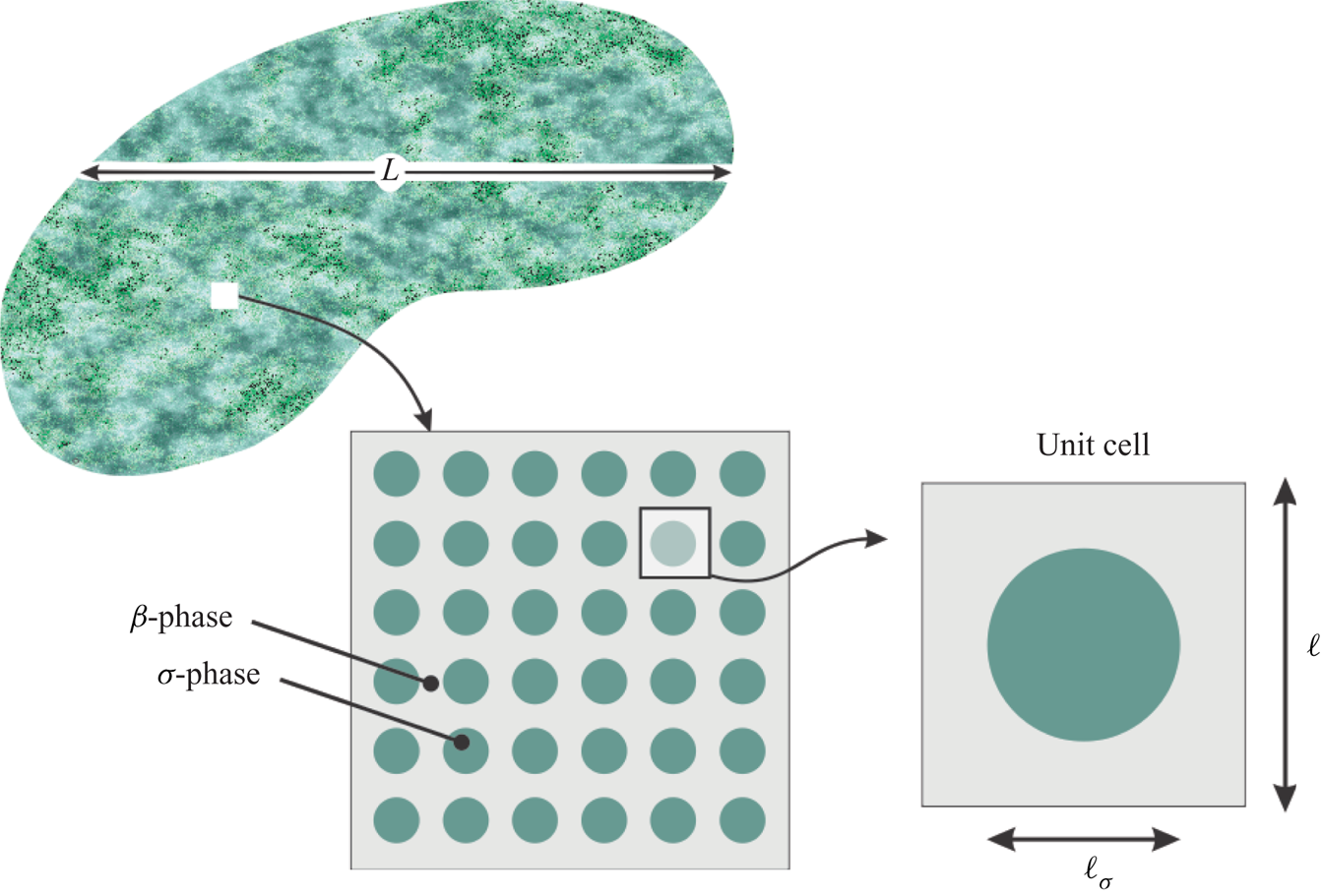
The purpose of this section is twofold. First, the temporal evolutions of the effective-medium coefficient,  ${\boldsymbol{\mathsf{K}}}_{st}$, and of the average term,
 $\boldsymbol {\alpha }_s$, are predicted from the closure problem solution in the simple geometric unit cell sketched in figure 2. Second, the predictions of the average velocity resulting from the upscaled model are validated by comparison with pore-scale numerical simulations. For the sake of simplicity, the computations were performed assuming incompressible flow. Before detailing the results, it is convenient to reformulate the closure problem and the upscaled model in terms of the following dimensionless variables and parameters:
 \begin{equation} \left.\begin{gathered} \boldsymbol{r}^*= \frac{\boldsymbol{r}}{\ell}; \quad t^* = \frac{\mu t}{\langle \rho \rangle^\beta \ell^2}; \quad {\boldsymbol{\mathsf{D}}}^* = \frac{{\boldsymbol{\mathsf{D}}}}{\ell^2}; \quad \boldsymbol{d}^* = \frac{\boldsymbol{d}}{\ell}; \quad \bar{\lambda}^*= \frac{\bar{\lambda}}{\ell}; \quad {\boldsymbol{\mathsf{K}}}_{st}^*= \frac{ {\boldsymbol{\mathsf{K}}}_{st}}{\ell^2},\\ \langle \boldsymbol{v}^*\rangle = \frac{ \langle \boldsymbol{v}\rangle}{v_{ref}}; \quad \boldsymbol{\alpha}_s^* = \frac{\boldsymbol{\alpha}_s}{v_{ref}}; \quad \boldsymbol{v}_0^* = \frac{\boldsymbol{v}_0}{v_{ref}}; \quad \langle p^* \rangle^\beta = \frac{\ell \langle p\rangle^\beta}{\mu v_{ref}}. \end{gathered}\right\} \end{equation}
Here,  $\ell$ is the side length of the periodic unit cell (see figure 2) and
 $v_{ref}={\ell ^2}/{\mu }\| \boldsymbol {\nabla } \langle p \rangle ^\beta \|$,
 $\| \boldsymbol {\nabla } \langle p \rangle ^\beta \|$ is the non-zero pressure gradient magnitude at a given arbitrary time. On the basis of the above definitions, the dimensionless version of the closure problem is written as
 \begin{gather} \boldsymbol{\nabla}^* \boldsymbol{\cdot} {\boldsymbol{\mathsf{D}}}^*=\boldsymbol{0}, \quad \text{in the}\ \beta\text{-phase},\ t^*>0, \end{gather}
 \begin{gather}\frac{\partial {\boldsymbol{\mathsf{D}}}^*}{\partial t^*} ={-}\boldsymbol{\nabla}^* \boldsymbol{d}^*+\boldsymbol{\nabla}^* \boldsymbol{\cdot} \left(\boldsymbol{\nabla}^* {\boldsymbol{\mathsf{D}}}^* +\boldsymbol{\nabla}^* {\boldsymbol{\mathsf{D}}}^{*{T}1}\right) + {\boldsymbol{\mathsf{I}}}, \quad \text{in the}\ \beta\text{-phase},\ t^*>0, \end{gather}
 \begin{gather}{\boldsymbol{\mathsf{D}}}^* ={-}\xi \bar{\lambda}^*\left( {\boldsymbol{\mathsf{I}}}-\boldsymbol{n}\boldsymbol{n}\right) \boldsymbol{\cdot} \left[ \boldsymbol{n}\boldsymbol{\cdot} \left(\boldsymbol{\nabla}^* {\boldsymbol{\mathsf{D}}}^*+ \boldsymbol{\nabla}^* {\boldsymbol{\mathsf{D}}}^{*{T}1}\right) \right], \quad \text{at }\mathscr{A}_{\beta\sigma},\ t^*>0, \end{gather}
 \begin{gather}\langle \boldsymbol{d}^*\rangle^\beta =\boldsymbol{0},\quad t^*>0, \end{gather}
 \begin{gather}\text{when } t^*=0, \quad {\boldsymbol{\mathsf{D}}}^*=\boldsymbol{0}, \end{gather}
 \begin{gather}\psi(\boldsymbol{r}^*+\boldsymbol{l}^*_i)=\psi(\boldsymbol{r}^*), \quad i=1,2,3; \quad \psi = {\boldsymbol{\mathsf{D}}}^*, \boldsymbol{d}^*. \end{gather}
This problem was numerically solved using the finite element software Comsol Multiphysics 5.6 using a segregated and direct solver. For the purposes of performing the numerical solution, the terms on the right-hand side of the slip condition given in (4.2c) were multiplied by a smooth and unitary step function at early dimensionless times (i.e. at  $t^*<10^{-9}$). After performing standard meshing tests, it was verified that the results were independent of this numerical degree of freedom. Once the closure problem solution was achieved, the results were substituted into the following dimensionless expressions:
 \begin{gather} {\boldsymbol{\mathsf{K}}}_{st}^*= \langle {\boldsymbol{\mathsf{D}}}^*\rangle, \end{gather}
 \begin{gather}\boldsymbol{\alpha}_s^* = \left\langle \boldsymbol{v}_0^* \boldsymbol{\cdot} \frac{\partial {\boldsymbol{\mathsf{D}}}^* }{\partial t^*} \right\rangle. \end{gather}
Note that in the first of the above equations, the symmetric nature of the tensor,  ${\boldsymbol{\mathsf{K}}}_{st}$, was taken into account. Finally, the dimensionless version of the upscaled model given in (3.29) can be written as
 \begin{equation} \langle\boldsymbol{v}^*\rangle ={-}\frac{\textrm{d} {\boldsymbol{\mathsf{K}}}_{st}^* }{\textrm{d} t^*}* \boldsymbol{\cdot} \,\boldsymbol{\nabla}\left\langle p^*\right\rangle^\beta +\boldsymbol{\alpha}_s^*. \end{equation}
In the following subsections, the dynamic behaviour of  ${\boldsymbol{\mathsf{K}}}_{st}^*$ and
 $\boldsymbol {\alpha }_s^*$ is presented and discussed.
Sketch of the periodic unit cell used to numerically solve the closure problem.

4.1. Dynamic effective coefficients
Due to the geometry of the solid inclusion in the unit cell, tensor  ${\boldsymbol{\mathsf{K}}}_{st}$ is isotropic and hence only the
 $xx$-component needs to be reported. In this context,
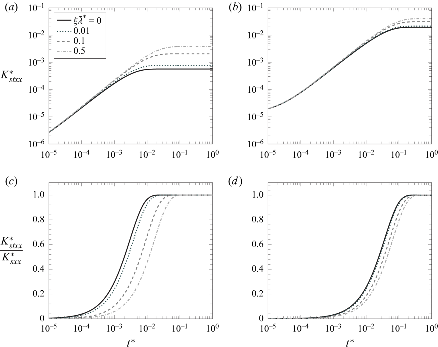
 $\boldsymbol {e}_x$ is taken as the unit vector along the horizontal axis of the unit cell sketched in figure 2. In figure 3, the results of
 $K^*_{stxx}$, as defined in (4.1), are represented versus the dimensionless time for two porosity values of the unit cell, namely
 $\varepsilon =0.4$ (figure 3a,c) and
 $\varepsilon =0.8$ (figure 3b,d), varying the slip coefficient
 $\xi \bar {\lambda }^*$ between 0.01 and 0.5.
Temporal evolution of the  $xx$-component of the dimensionless apparent dynamic permeability tensor resulting from solving the closure problem (4.2) in the unit cell sketched in figure 2 with
 $\varepsilon = 0.4$ in panels (a,c) and
 $\varepsilon = 0.8$ in panels (b,d), for different values of
 $\xi \bar {\lambda }^*$. Results in panels (c,d) are normalized with respect to the steady-state value,
 $K^*_{sxx}$.

The closure problem given in (4.2) shows that the field of  ${\boldsymbol{\mathsf{D}}}^*$ departs from a zero initial value and increases over time, until reaching a steady-state value, which agrees with that reported by Lasseux et al. (Reference Lasseux, Valdés-Parada and Porter2016). As a consequence, the evolution of
 $K^*_{stxx}$ reported in figure 3 (from 0 to
 $K^*_{sxx}$) is expected and consistent with the proof provided in Appendix D. Note that, at sufficiently small times, all the curves converge onto a single one as expected from the initial condition for the closure problem. Moreover, the time at which slip effects become significant in the dynamics of the apparent permeability decreases as the porosity decreases.
The values of  $K_{stxx}^*$ increase with
 $\xi \bar {\lambda }^*$ and, for
 $\varepsilon =0.4$, the influence of slip is more pronounced than for
 $\varepsilon =0.8$. Interestingly, the time at which steady state is reached increases with
 $\xi \bar {\lambda }^*$. To better appreciate this effect, in figure 3(c,d), results are presented normalized with respect to the steady-state value (
 $K^*_{sxx}$). These results clearly show that interfacial slip tends to increase the time rate of change of the apparent dynamic permeability, and this is easier to observe in figure 3(a) corresponding to
 $\varepsilon =0.4$. In this particular case, the time to reach steady state for the largest slip (i.e.
 $\xi \bar {\lambda }^*=0.5$) exhibits a delay of approximately one order of magnitude with respect to the no-slip case. In contrast, for
 $\varepsilon =0.8$, this characteristic time value is only doubled. For a given value of
 $\xi \bar {\lambda }^*$, the time at which
 $K_{stxx}^*$ reaches its steady value, i.e. the relaxation time, is larger when the porosity increases. To summarize, the dependence of the relaxation time on both the porosity and
 $\xi \bar {\lambda }^*$ can be explained by the fact that viscous drag (thus viscous dissipation) decreases when slip effects increase and porosity increases and hence the viscous relaxation time is lengthened. Finally, it must noted that the characteristic dimensionless time for
 $K_{stxx}$ to reach steady state is not necessarily of order 1. This is expected since the choice of the time reference based on the unit cell size does not represent an exact measure of the viscous relaxation time, which depends on slip effects and porous structure. In fact, the latter has a considerable impact since this relaxation time decreases by approximately one order of magnitude when the porosity is decreased from 0.8 to 0.4 for the geometry under consideration here. A relaxation time for
 $K_{stxx}^*$ close to the pore-scale viscous relaxation time,
 $\langle \rho \rangle ^\beta \ell ^2/\mu$, (or even larger due to slip effects) may be expected for a porosity value close to 1. This can be illustrated by considering a simple structure made of a periodic repetition of plane-parallel plates oriented along
 $\boldsymbol {e}_x$. In that case,
 $K_{stxx}^*$ can be obtained analytically. It is given by
 \begin{equation} K_{stxx}^* = \frac{\varepsilon^3}{12} +\frac{\varepsilon^2}{2} \xi \bar{\lambda}^* +2\sum_{n=1}^\infty \frac{A_n}{\beta_n} \sin\left(\beta_n \frac{\ell_\beta^*}{2} \right) \textrm{e}^{-\beta_n^2 t^*}. \end{equation}
In this relationship,  $\beta _n$ are the eigenvalues resulting from the solution of the following equation:
 \begin{equation} \cos\left(\beta_n\frac{ \ell_\beta^*}{2} \right) = \xi \bar{\lambda}^* \beta_n \sin\left(\beta_n \frac{ \ell_\beta^*}{2} \right), \end{equation}
and the coefficient  $A_n$ is
 \begin{equation} A_n={-} \frac{ \sin(\beta_n \ell_\beta^*/2 )}{\beta_n^3\| \varphi_n \|^2 }, \end{equation}
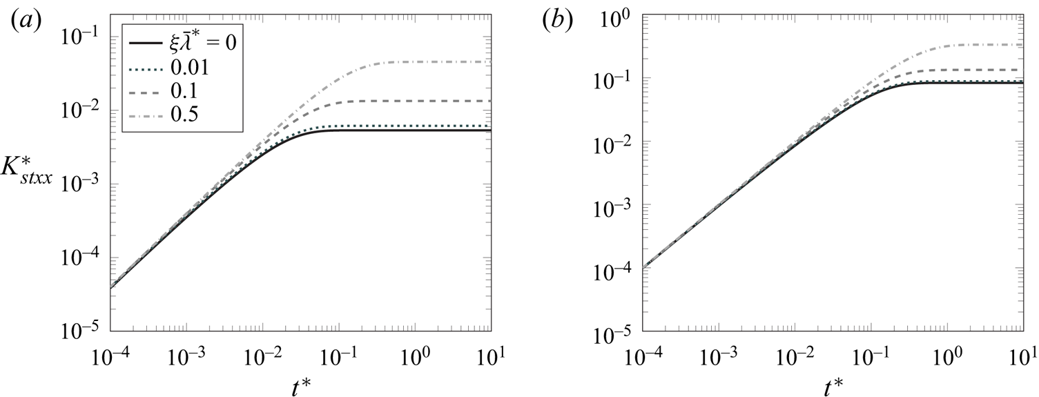
where  $\|\varphi _n\|^2={\ell _\beta ^*}(1 + {2\xi \bar {\lambda }^* }/({ \ell _\beta ^* [(\beta _n\xi \bar {\lambda }^*)^2+1 ]}))/4$. As shown in figure 4(a), for
 $\varepsilon =0.4$,
 $K_{stxx}^*$ behaves the same as for the structure made of parallel cylinders and its dimensionless relaxation time is comparable. However, when the porosity is close to 1, as in figure 4(b), the steady value is reached at
 $t^*\simeq 0.7$ under no-slip conditions and
 $t^*\simeq 2$ for
 $\xi \bar {\lambda }^*=0.5$.
Temporal evolution of the  $xx$-component of the dimensionless apparent dynamic permeability tensor resulting from the analytical solution of the closure problem in a unit cell consisting of two parallel plates with (a)
 $\varepsilon =0.4$ and (b)
 $\varepsilon =0.999$, for different values of
 $\xi \bar {\lambda }^*$.

Directing attention to the computation of  $\boldsymbol {\alpha }_s^*$, (4.3b) shows that its values depend upon the choice of the initial condition of the pore-scale velocity,
 $\boldsymbol {v}_0^*$. In figure 5, as well as in the remainder of this work, for the sake of simplicity, results are reported taking
 $\boldsymbol {v}_0^*$ as the solution of the following dimensionless flow problem:
 \begin{gather} \boldsymbol{\nabla}^* \boldsymbol{\cdot} \boldsymbol{v}_0^* =0, \quad \text{in the}\ \beta\text{-phase}, \end{gather}
 \begin{gather}\boldsymbol{0}={-}\boldsymbol{\nabla}^* \tilde{p}_0^* + \boldsymbol{\nabla}^* \boldsymbol{\cdot} \left( \boldsymbol{\nabla}^* \boldsymbol{v}_0^* + \boldsymbol{\nabla}^* \boldsymbol{v}_0^{*T} \right) - \boldsymbol{\nabla}^* \langle p_0^* \rangle^\beta , \quad \text{in the}\ \beta\text{-phase}, \end{gather}
 \begin{gather}\boldsymbol{v}_0^* ={-}\xi \bar{\lambda}^* ({\boldsymbol{\mathsf{I}}}-\boldsymbol{n}\boldsymbol{n}) \boldsymbol{\cdot} \left[ \boldsymbol{n} \boldsymbol{\cdot} \left( \boldsymbol{\nabla}^* \boldsymbol{v}_0^* +\boldsymbol{\nabla}^* \boldsymbol{v}_0^{*T} \right) \right], \quad \text{at }\mathscr{A}_{\beta \sigma}, \end{gather}
 \begin{gather}\langle \tilde{p}_0^* \rangle^\beta =0, \end{gather}
 \begin{gather}\psi (\boldsymbol{r}^*+\boldsymbol{l}_i^*)= \psi (\boldsymbol{r}^*), \quad i=1,2,3; \quad \psi = \boldsymbol{v}_0^*, \tilde{p}_0^*. \end{gather}
In (4.8b), the macroscopic pressure gradient was taken to be  $\boldsymbol {\nabla }^* \langle p_0^* \rangle ^\beta = -0.1 \,\boldsymbol {e}_x$. This value of the initial macroscopic pressure gradient is chosen for the sake of consistency with the analysis presented in § 4.2. It should be noted that, since
 $\boldsymbol {v}_0^*$ obeys the Stokes problem given in (4.8),
 $\boldsymbol {\alpha }_s^*$ corresponds to the dimensionless form of the last term on the right-hand side of (3.32). Nevertheless, it is of interest to analyse the influence of interfacial slip on the temporal dependence of
 $\boldsymbol {\alpha }_s^*$.
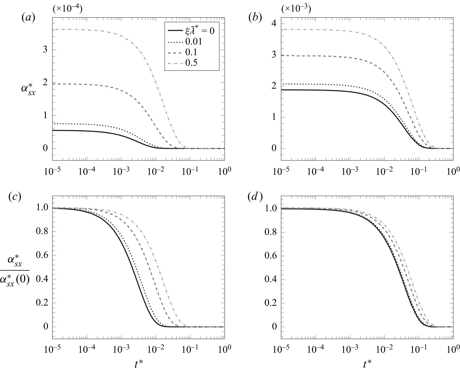
Temporal evolution of the  $x$-component of the dimensionless vector
 $\boldsymbol {\alpha }_s$. In panels (a,c),
 $\varepsilon = 0.4$; in panels (b,d),
 $\varepsilon = 0.8$. Results in panels (c,d) are normalized with respect to their respective initial values.

The results reported in figure 5 are presented in a similar fashion as those for  $K^*_{stxx}$, i.e. in figure 5(a,b),
 $\alpha ^*_{sx}$, as defined in (4.1), is represented versus
 $t^*$ in order to appreciate the effect of interfacial slip. In figure 5(c,d),
 $\alpha ^*_{sx}$ is normalized by its initial value,
 $\alpha ^*_{sx}(0)$, in order to better highlight the slip effect on the dynamics of this effective term, in particular, the time interval over which it plays a significant role on the flow.
The sigmoidal and time-decreasing shape down to zero of the predictions shown in figure 5 are physically sound. In fact, according to (4.3b),  $\boldsymbol {\alpha }_s^*$ is the average of the inner product of the dimensionless initial fluid velocity and the time derivative of the closure variable
 ${\boldsymbol{\mathsf{D}}}^*$. The latter derivative is equal to
 ${\boldsymbol{\mathsf{I}}}$ at
 $t^*=0$ and asymptotically reaches zero at steady state.
As expected,  $\alpha ^*_{sx}$ increases with
 $\xi \bar {\lambda }^*$ and the influence is more significant for
 $\varepsilon = 0.4$. Indeed, the magnitude of
 $\alpha ^*_{sx}$ is intimately linked to the initial condition of the velocity. Nevertheless, as indicated by the evolution of
 $\alpha ^*_{sx}/\alpha ^*_{sx}(0)$ represented in figure 5(c,d), the impact of slip on this effective term is more pronounced for small porosities. In addition, these results show that the presence of slip increases the time of action of this memory term, particularly for small
 $\varepsilon$. Consistently with the results shown in figure 3(c,d), the characteristic time at which
 $\alpha _{sx}^*$ approaches zero increases by approximately one order of magnitude for
 $\varepsilon =0.4$, and is only doubled for
 $\varepsilon =0.8$, when
 $\xi \bar {\lambda }^*$ goes from 0 to 0.5.
4.2. Upscaled model versus direct numerical simulations on a case study
To conclude this section, the predictions of the average velocity resulting from the dimensionless upscaled model, as written in (4.4), are compared, in the following paragraphs, with the results of DNS of the dimensionless pore-scale flow problem using a prescribed macroscopic pressure gradient. The purpose here is not to provide an exhaustive examination of responses to several macroscopic pressure gradient expressions. Rather, the objective is to validate the model with in silico experiments for a particular flow situation. Among many possible alternatives for  $\boldsymbol {\nabla }^*\langle p^* \rangle ^\beta$ (see e.g. § 4 in the work of Lasseux et al. Reference Lasseux, Valdés-Parada and Bellet2019), the idea is to use a time dependent forcing leading to periodic flow regimes. With this in mind, the following dimensionless macroscopic pressure gradient in the horizontal direction is chosen:
 \begin{equation} -\frac{\textrm{d} \langle p^* \rangle^\beta}{{\textrm{d} x}^*}= \begin{cases} 0.1, & t^* \leqslant 0, \\ 0.6-0.5 \cos (\omega^* t^*), & t^* > 0. \end{cases} \end{equation}
Note that no macroscopic pressure gradient is applied in the vertical direction, that the function is continuous at  $t^*=0$ and that the initial condition is consistent with that used in the predictions of
 $\boldsymbol {\alpha }_s^*$ reported above. In the above equation, the value of
 $\omega ^*$ was fixed to
 $10^3$ and
 $10^2$ for the simulations presented below. It is worth mentioning that in an infinitely periodic porous medium, the DNS solution can be performed in only a single unit cell and in this case, the matching between the upscaled model and in silico experiments is guaranteed.
To carry out the comparison using a finite-size domain, DNS of the pore-scale flow problem, as given by the incompressible (dimensionless) version of (2.1), were performed in a horizontal array of  $N$ unit cells and the average velocity was computed over the central one. Periodic boundary conditions on
 $\boldsymbol {v}^*$ and
 $\tilde {p}^*$ were applied in the
 $y$-direction. The macroscopic boundary conditions in the
 $x$-direction were the following:
 \begin{gather} \text{at } x^*=0, \quad \langle p^*\rangle^\beta ={-}N \frac{\textrm{d} \langle p^*\rangle^\beta}{{\textrm{d} x}^*} , \end{gather}
 \begin{gather}\text{at } x^*=N, \quad \langle p^*\rangle^\beta =0. \end{gather}
In this way, each one of the  $N$ unit cells experiences the dimensionless pressure gradient given in (4.9). Note that due to incompressibility, it follows that
 $\xi \lambda ^*=\xi \bar {\lambda }^*$. The number of unit cells used in the pore-scale simulations was fixed to
 $N=21$ after verifying that results were unchanged upon varying the number of unit cells. The porosity was set to
 $\varepsilon =0.4$.
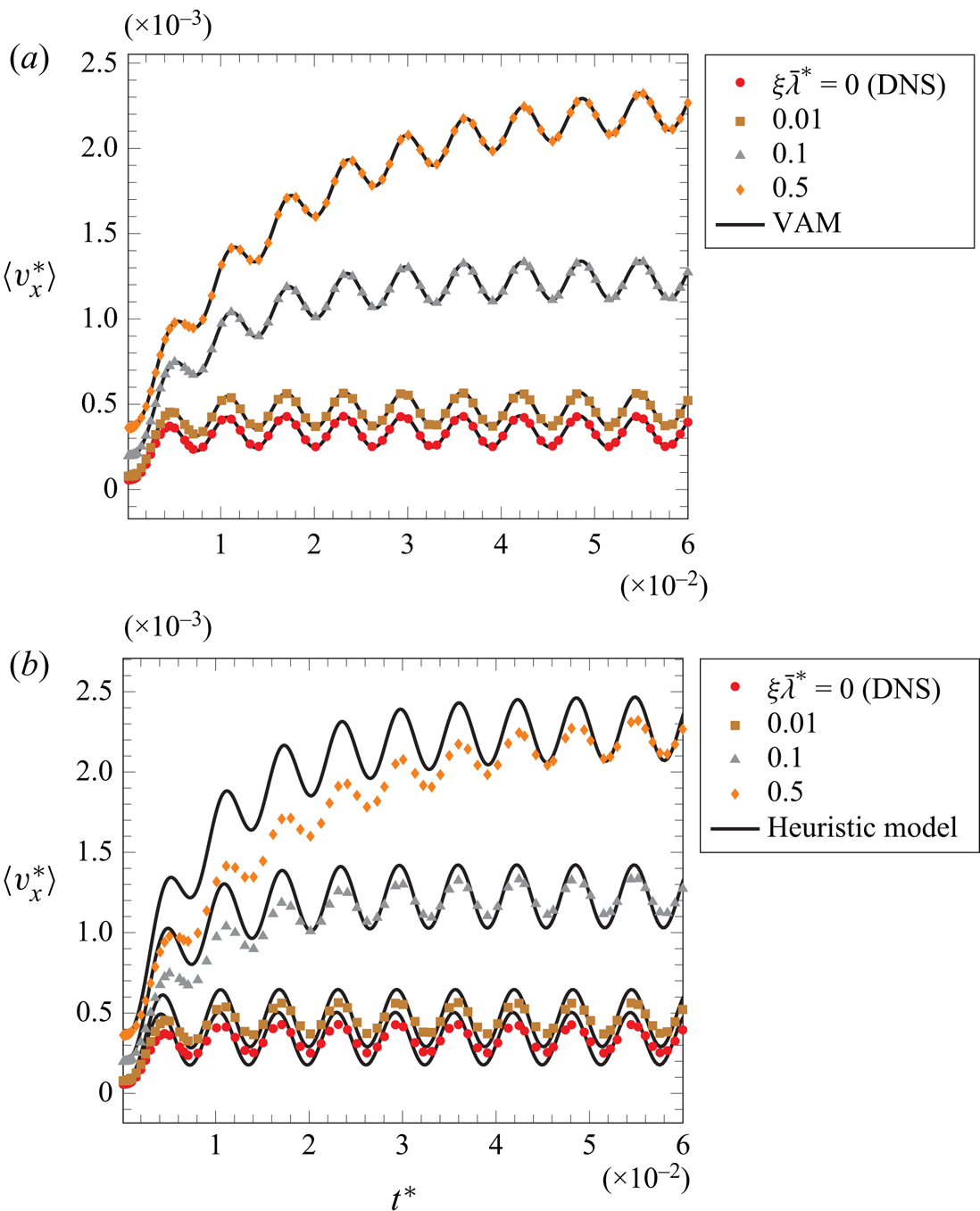
In figure 6(a), the velocity profiles resulting from DNS are compared with the predictions from the VAM given in (4.4) for  $\omega ^*=10^3$. In order to carry out the convolution product in the upscaled model, the dynamics of
 $K_{stxx}^*$ were fitted using exponential functions. This allowed computing analytically the convolution integral. As an alternative, numerical quadratures could also have been used to compute the convolution product. Consequently the computational time required to evaluate the upscaled model derived here was considerably smaller than that required to perform DNS. As expected from the previous results, the average velocity increases with
 $\xi \bar {\lambda }^*$ and the characteristic time at which a permanent oscillatory regime is established is delayed as
 $\xi \bar {\lambda }^*$ is increased. More importantly, it can be observed that the average velocity results predicted by the VAM perfectly reproduces those obtained from DNS. In fact, the relative error between modelling approaches remains below 2 % in all the cases under consideration, which validates the upscaled model derived in this work.
Temporal evolution of the  $x$-component of the dimensionless macroscale velocity resulting from considering an oscillatory macroscopic pressure gradient. Comparison of the results obtained from DNS with (a) the volume-averaged model (VAM) and (b) the heuristic model. Results are reported for different values of the slip coefficient
 $\xi \bar {\lambda }^*$, for
 $\varepsilon =0.4$ and
 $\omega ^*= 10^3$.

As a final point of analysis, it is worth evaluating the performance of the dimensionless heuristic model given by
 \begin{equation} \frac{\textrm{d} \langle \boldsymbol{v}^*\rangle^\beta }{\textrm{d}t^*} ={-}\boldsymbol{\nabla}^* \langle p^* \rangle^\beta -\varepsilon {\boldsymbol{\mathsf{K}}}_{s}^{*-1}\boldsymbol{\cdot} \langle \boldsymbol{v}^*\rangle^\beta , \quad t^*>0. \end{equation}
Here, again,  ${\boldsymbol{\mathsf{K}}}_{s}^{*}$ is the steady-state value of the apparent dynamic permeability tensor,
 ${\boldsymbol{\mathsf{K}}}_{st}^{*}$. In addition, the above equation is subject to the following initial condition:
 \begin{equation} \text{when }t^*=0, \quad \langle \boldsymbol{v}^* \rangle= \langle \boldsymbol{v}_0^* \rangle. \end{equation}
This model is the result of assuming that the pore-scale flow is quasi-steady with respect to the macroscopic fluid motion. However, this assumption is difficult to justify as both time scales are of the same order of magnitude (see e.g. Whitaker Reference Whitaker1996). Hence, in general, the heuristic model can be expected to only partially capture the macroscopic flow dynamics. In particular, it is unlikely to appropriately reproduce it at any time shorter than the viscous relaxation time at the pore-scale, or whenever the macroscopic pressure gradient is varying over a characteristic period shorter than this relaxation time.
Since the macroscopic pressure gradient is applied in the  $x$-direction, the only non-zero component of the average velocity is the horizontal one, along
 $\boldsymbol {e}_x$. Using the expression of
 ${\textrm {d} \langle p^* \rangle ^\beta }/{{\textrm {d} x}^*}$ given in (4.9), the analytical solution of the above problem for
 $\langle v_x^*\rangle$ is
 \begin{align} \langle v_x^*\rangle &= \langle v_{0x}^*\rangle \exp (-\varepsilon t^* /K_{sxx}^*) + 0.6 K_{sxx}^* \left[ 1-\exp (-\varepsilon t^* /K_{sxx}^*)\right] \nonumber\\ &\quad - \frac{0.5K_{sxx}^{*} }{1+ \left( \dfrac{\omega^{*} K_{sxx}^* }{\varepsilon}\right)^2 } \left[ \cos(\omega^* t^*) + \frac{\omega^* K_{sxx}^*}{\varepsilon} \sin(\omega^* t^*)- \exp (-\varepsilon t^* /K_{sxx}^*) \right]. \end{align}
The comparison of the predictions resulting from this expression with DNS results is reported in figure 6(b). Clearly, the heuristic model does not reproduce adequately the velocity obtained from DNS. The largest deviations occur before regular time-periodic oscillations are reached, and are more easily observable with the increase of  $\xi \bar {\lambda }^*$. Moreover, it can be observed that the prediction from the heuristic model of the characteristic time at which the periodic regime is obtained is much smaller than the actual one. These observations are consistent with those reported by Lasseux et al. (Reference Lasseux, Valdés-Parada and Bellet2019) under no slip and inertial conditions and confirm that the heuristic model is not adequate, in general, to reproduce the macroscale velocity dynamics. The average velocity, obtained in the same conditions as those considered for the results reported in figure 6, with
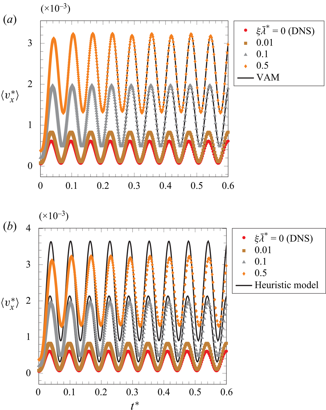
 $\omega ^*=10^2$, is represented versus time in figure 7. In that case, the oscillating period of
 $\boldsymbol {\nabla }^*\langle p^*\rangle ^\beta$ is comparable to the relaxation time of
 $K_{stxx}^*$, at least for
 $\xi \bar {\lambda }^*$ smaller than 0.1. As can be seen in this figure, the prediction of the VAM is again in perfect agreement with the DNS results (see figure 7a). Figure 7(b) shows that the heuristic model reproduces correctly the macroscopic flow for values of
 $\xi \bar {\lambda }^*$ smaller than the threshold value of 0.1. For more important slip effects, a clear discrepancy occurs and is maintained over time.
Temporal evolution of the  $x$-component of the dimensionless macroscale velocity resulting from considering an oscillatory macroscopic pressure gradient. Comparison of the results obtained from DNS with (a) the VAM and (b) the heuristic model. Results are reported for different values of the slip coefficient
 $\xi \bar {\lambda }^*$,
 $\varepsilon =0.4$ and
 $\omega ^*= 10^2$.

5. Conclusions
In this work, a macroscopic model was derived to describe unsteady and single-phase, slightly compressible creeping flow with interfacial slip conditions through homogeneous porous media, by upscaling the pore-scale governing equations. Slip at the boundary was treated by the use of a Navier-type equation, which may account for rarefied gas conditions as well as for the effective behaviour of the fluid in the proximity of rough surfaces. The macroscopic equation for mass conservation keeps a similar form as its pore-scale counterpart, whereas the macroscopic momentum transport equation does not correspond to the heuristic model commonly found in the literature. This equation contains two terms, the first consists of a convolution product between the temporal derivative of the apparent dynamic permeability tensor ( ${\boldsymbol{\mathsf{K}}}_{st}$) and the macroscopic pressure gradient. The second term,
 $\boldsymbol {\alpha }_s$, is a memory term that accounts for the influence of the initial flow at the pore-scale.
The model was derived following a volume averaging procedure fully consistent with the adjoint homogenization strategy proposed by Bottaro (Reference Bottaro2019). The approach is novel in the sense that it departs from the fundamental problem for the velocity Green's function pair associated to the flow equation written in a periodic unit cell. Then, from the use of Green's formula, it directly leads to the upscaled momentum transport equation. A salient feature of this approach is that it only requires the solution of one closure problem in order to compute the values of  ${\boldsymbol{\mathsf{K}}}_{st}$ and
 $\boldsymbol {\alpha }_s$, independently of the initial flow distribution and macroscopic pressure gradient. Furthermore, from the analysis of the closure problem, it was concluded that the apparent dynamic permeability tensor is symmetric despite the presence of interfacial slip.
The numerical solution of the closure problem allowed prediction of the dynamics of  ${\boldsymbol{\mathsf{K}}}_{st}$ and
 $\boldsymbol {\alpha }_s$ in particular flow conditions. Numerical simulations led to conclude that the apparent dynamic permeability increases at all times until its final steady-state value is reached. For a given configuration of the solid phase in the unit cell, the relaxation time of
 ${\boldsymbol{\mathsf{K}}}_{st}$ to its steady value increases with both porosity and slip effects. This is attributed to the fact that viscous dissipation decreases under these conditions and, as a consequence, the viscous relaxation time is lengthened. In addition, the magnitude of
 $\boldsymbol {\alpha }_s$ and the time range over which this memory term plays a role in the macroscopic momentum equation are amplified due to the slip effects.
Finally, the model predictions were validated by comparison with direct numerical simulations in which the pressure gradient is oscillatory. The average velocity resulting from pore-scale simulations and predicted from the upscaled model were found to be in excellent agreement. In contrast, the heuristic macroscopic model could not reproduce the results obtained from in silico experiments whenever the characteristic time of variation of the pressure gradient is smaller than the relaxation time of the apparent dynamic permeability. This leads to conclude that such a model is not adequate, in general, to study unsteady flow in porous media.
The results from this work represent an important new contribution in upscaling momentum transport in porous media under unsteady slip conditions. The findings reported should motivate further experimental and theoretical research where this situation arises or even when it is coupled to other transport phenomena.
Declaration of interests
The authors report no conflict of interest.
Appendix A
The objective of this appendix is to demonstrate Green's formula given in (3.15), i.e.
 \begin{align} & \int_{\mathscr{V}_\beta} \left[\boldsymbol{q} \boldsymbol{\cdot} \left(\boldsymbol{\nabla} \boldsymbol{\cdot} \left( \boldsymbol{\nabla} {\boldsymbol{\mathsf{M}}} + \boldsymbol{\nabla} {\boldsymbol{\mathsf{M}}}^{{T}1} \right) \right) - \left(\boldsymbol{\nabla} \boldsymbol{\cdot} \left( \boldsymbol{\nabla}\boldsymbol{q}+\boldsymbol{\nabla} \boldsymbol{q}^T \right)\right)\boldsymbol{\cdot}{\boldsymbol{\mathsf{M}}} \right]\textrm{d}V \nonumber\\ &\quad =\int_{\mathscr{A}_\beta} \boldsymbol{n} \boldsymbol{\cdot} \left[\boldsymbol{q} \boldsymbol{\cdot} \left( \boldsymbol{\nabla} {\boldsymbol{\mathsf{M}}} + \boldsymbol{\nabla} {\boldsymbol{\mathsf{M}}}^{{T}1} \right) - \left( \boldsymbol{\nabla}\boldsymbol{q}+\boldsymbol{\nabla} \boldsymbol{q}^T \right)\boldsymbol{\cdot} {\boldsymbol{\mathsf{M}}} \right]\textrm{d}A, \end{align}
where  $\mathscr {A}_\beta$ represents all the surfaces bounding
 $\mathscr {V}_\beta$ within the unit cell, i.e.
 $\mathscr {A}_\beta =\mathscr {A}_{\beta \sigma }+\mathscr {A}_{\beta e}$,
 $\mathscr {A}_{\beta e}$ being the entrance and exit surfaces of
 $\mathscr {V}_{\beta }$ at the edges of the unit cell.
Preliminary tools to carry out the proof of this relationship are the following identities, which are valid for any vector  $\boldsymbol {u}$, second-order tensors
 ${\boldsymbol{\mathsf{U}}}$ and
 ${\boldsymbol{\mathsf{V}}}$, and third-order tensor
 ${\boldsymbol{\mathsf{W}}}$:
 \begin{gather} \boldsymbol{\nabla}\boldsymbol{\cdot}\left(\boldsymbol{u}\boldsymbol{\cdot}{\boldsymbol{\mathsf{W}}}\right)= \boldsymbol{\nabla} \boldsymbol{u}:{\boldsymbol{\mathsf{W}}}+\boldsymbol{u} \boldsymbol{\cdot} \left(\boldsymbol{\nabla}\boldsymbol{\cdot}{\boldsymbol{\mathsf{W}}}^{{T}1}\right), \end{gather}
 \begin{gather}\boldsymbol{\nabla} \boldsymbol{\cdot}({\boldsymbol{\mathsf{U}}}\boldsymbol{\cdot}{\boldsymbol{\mathsf{V}}})=\left(\boldsymbol{\nabla} \boldsymbol{\cdot}{\boldsymbol{\mathsf{U}}}\right)\boldsymbol{\cdot}{\boldsymbol{\mathsf{V}}}+{\boldsymbol{\mathsf{U}}}^T:\boldsymbol{\nabla} {\boldsymbol{\mathsf{V}}}, \end{gather}
 \begin{gather}{\boldsymbol{\mathsf{U}}}^T:{\boldsymbol{\mathsf{W}}}={\boldsymbol{\mathsf{U}}}:{\boldsymbol{\mathsf{W}}}^{{T}1}. \end{gather}
In the above identities, the symbol  $:$ is the double dot product, defined in accordance with the nesting convention adopted throughout this work, i.e. for instance,
 $(\boldsymbol {\nabla } \boldsymbol {u}:{\boldsymbol{\mathsf{W}}})_k=(\boldsymbol {\nabla } u)_{ij} W_{jik}$, where the Einstein notation is implied.
Identifying  $\boldsymbol {u}$ to
 $\boldsymbol {q}$ and
 ${{\boldsymbol{\mathsf{W}}}}$ to
 $(\nabla {\boldsymbol{\mathsf{M}}}+\boldsymbol {\nabla }{\boldsymbol{\mathsf{M}}}^{{T}1})$ in (A2a) allows writing
 \begin{equation} \boldsymbol{\nabla} \boldsymbol{\cdot}\left(\boldsymbol{q} \boldsymbol{\cdot} \left( \boldsymbol{\nabla} {\boldsymbol{\mathsf{M}}} + \boldsymbol{\nabla} {\boldsymbol{\mathsf{M}}}^{{T}1} \right) \right) =\boldsymbol{\nabla} \boldsymbol{q}:\left(\boldsymbol{\nabla} {\boldsymbol{\mathsf{M}}} + \boldsymbol{\nabla} {\boldsymbol{\mathsf{M}}}^{{T}1} \right) +\boldsymbol{q}\boldsymbol{\cdot}\left( \boldsymbol{\nabla}\boldsymbol{\cdot}\left( \boldsymbol{\nabla} {\boldsymbol{\mathsf{M}}} + \boldsymbol{\nabla} {\boldsymbol{\mathsf{M}}}^{{T}1}\right)\right). \end{equation}
Similarly, identifying  ${{\boldsymbol{\mathsf{U}}}}$ to
 $(\boldsymbol {\nabla } \boldsymbol {q}+\boldsymbol {\nabla }\boldsymbol {q}^T)$ and
 ${{\boldsymbol{\mathsf{V}}}}$ to
 ${\boldsymbol{\mathsf{M}}}$ in (A2b) yields
 \begin{equation} \boldsymbol{\nabla}\boldsymbol{\cdot}\left(\left(\boldsymbol{\nabla} \boldsymbol{q}+ \boldsymbol{\nabla}\boldsymbol{q}^T\right)\boldsymbol{\cdot} {\boldsymbol{\mathsf{M}}}\right) =\left(\boldsymbol{\nabla}\boldsymbol{\cdot}\left(\boldsymbol{\nabla} \boldsymbol{q}+ \boldsymbol{\nabla}\boldsymbol{q}^T\right)\right)\boldsymbol{\cdot} {\boldsymbol{\mathsf{M}}} +\left(\boldsymbol{\nabla} \boldsymbol{q}+\boldsymbol{\nabla}\boldsymbol{q}^T \right): \boldsymbol{\nabla} {\boldsymbol{\mathsf{M}}}, \end{equation}
or, while making use of (A2c) in which  ${{\boldsymbol{\mathsf{U}}}}$ is taken as
 $\boldsymbol {\nabla } \boldsymbol {q}$ and
 ${{\boldsymbol{\mathsf{W}}}}$ as
 $\boldsymbol {\nabla } {\boldsymbol{\mathsf{M}}}$,
 \begin{equation} \boldsymbol{\nabla} \boldsymbol{\cdot}\left(\left(\boldsymbol{\nabla} \boldsymbol{q}+\boldsymbol{\nabla}\boldsymbol{q}^T\right)\boldsymbol{\cdot} {\boldsymbol{\mathsf{M}}}\right) =\left(\boldsymbol{\nabla}\boldsymbol{\cdot}\left(\boldsymbol{\nabla} \boldsymbol{q}+\boldsymbol{\nabla}\boldsymbol{q}^T\right)\right)\boldsymbol{\cdot} {\boldsymbol{\mathsf{M}}} +\boldsymbol{\nabla} \boldsymbol{q}:\left(\boldsymbol{\nabla} {\boldsymbol{\mathsf{M}}}+\boldsymbol{\nabla}{\boldsymbol{\mathsf{M}}}^{{T}1}\right). \end{equation}
Subtracting (A3c) from (A3a), integrating the result over  $\mathscr {V}_\beta$ and making use of the divergence theorem leads to the general Green's formula expressed in (A1).
In the present work, a special expression of this formula, given in (3.16), can be achieved, as shown below. The proof of this special form reduces to demonstrating that, for the physical problem under consideration, the area integral on the right-hand side of (A1) is zero.
Due to the fact that both  $\boldsymbol {q}$ and
 ${\boldsymbol{\mathsf{M}}}$ are periodic, the part of this area integral over
 $\mathscr {A}_{\beta e}$ is obviously zero. The proof hence amounts to demonstrating that
 \begin{equation} \int_{\mathscr{A}_{\beta\sigma}} \boldsymbol{n} \boldsymbol{\cdot} \left[\boldsymbol{q} \boldsymbol{\cdot} \left( \boldsymbol{\nabla} {\boldsymbol{\mathsf{M}}} + \boldsymbol{\nabla} {\boldsymbol{\mathsf{M}}}^{{T}1} \right) - \left( \boldsymbol{\nabla}\boldsymbol{q}+\boldsymbol{\nabla} \boldsymbol{q}^T \right)\boldsymbol{\cdot} {\boldsymbol{\mathsf{M}}} \right]\textrm{d}A =\boldsymbol{0}. \end{equation}
With the purpose of simplifying notations, the following nomenclature is adopted:
 \begin{gather} {\boldsymbol{\mathsf{A}}}=\boldsymbol{\nabla} \boldsymbol{q}+\boldsymbol{\nabla} \boldsymbol{q}^T, \end{gather}
 \begin{gather}{\boldsymbol{\mathsf{B}}}=\boldsymbol{\nabla} {\boldsymbol{\mathsf{M}}}+\boldsymbol{\nabla} {\boldsymbol{\mathsf{M}}}^{{T}1}, \end{gather}
 \begin{gather}{\boldsymbol{\mathsf{P}}}={\boldsymbol{\mathsf{I}}}-\boldsymbol{n}\boldsymbol{n}. \end{gather}
It should be noted that  ${\boldsymbol{\mathsf{A}}}$ and
 ${\boldsymbol{\mathsf{P}}}$ are second-order tensors, whereas
 ${\boldsymbol{\mathsf{B}}}$ is a third-order tensor. They satisfy the following symmetry conditions:
 \begin{gather} {\boldsymbol{\mathsf{A}}}={\boldsymbol{\mathsf{A}}}^T, \end{gather}
 \begin{gather}{\boldsymbol{\mathsf{P}}}={\boldsymbol{\mathsf{P}}}^T, \end{gather}
 \begin{gather}{\boldsymbol{\mathsf{B}}}={\boldsymbol{\mathsf{B}}}^{{T}1}. \end{gather}
As a consequence of this last relationship, it can be shown that, for any vector  $\boldsymbol {u}$, the following identity applies:
 \begin{equation} \boldsymbol{u}\boldsymbol{\cdot} {\boldsymbol{\mathsf{B}}}={\boldsymbol{\mathsf{B}}}^{{T}2}\boldsymbol{\cdot} \boldsymbol{u}, \end{equation}
where the superscript  ${T}2$ represents the transpose of a third-order tensor, which permutes the second and third indices, i.e.
 ${\boldsymbol{\mathsf{B}}}^{{T}2}_{ijk}={\boldsymbol{\mathsf{B}}}_{ikj}$.
Using the boundary conditions for  $\boldsymbol {q}$ and
 ${\boldsymbol{\mathsf{M}}}$ at
 $\mathscr {A}_{\beta \sigma }$, respectively given in (3.11c) and (3.14c), the integrand on the left-hand side of (A4) takes the following form:
 \begin{equation} \boldsymbol{n}\boldsymbol{\cdot} \left(\boldsymbol{q}\boldsymbol{\cdot}{\boldsymbol{\mathsf{B}}}-{\boldsymbol{\mathsf{A}}}\boldsymbol{\cdot} {\boldsymbol{\mathsf{M}}}\right) =\xi \bar{\lambda}\boldsymbol{n}\boldsymbol{\cdot}\left[{\boldsymbol{\mathsf{A}}}\boldsymbol{\cdot} {\boldsymbol{\mathsf{P}}}\boldsymbol{\cdot}\left(\boldsymbol{n}\boldsymbol{\cdot}{\boldsymbol{\mathsf{B}}}\right) -\left({\boldsymbol{\mathsf{P}}}\boldsymbol{\cdot}\left(\boldsymbol{n}\boldsymbol{\cdot}{\boldsymbol{\mathsf{A}}}\right)\right)\boldsymbol{\cdot}{\boldsymbol{\mathsf{B}}} \right]. \end{equation}
Employing the property indicated in (A6d) in which  $\boldsymbol {u}$ is identified as
 ${\boldsymbol{\mathsf{P}}}\boldsymbol {\cdot }(\boldsymbol {n}\boldsymbol {\cdot }{\boldsymbol{\mathsf{A}}})$, this last relationship can be equivalently expressed as
 \begin{equation} \boldsymbol{n}\boldsymbol{\cdot} \left(\boldsymbol{q}\boldsymbol{\cdot}{\boldsymbol{\mathsf{B}}}-{\boldsymbol{\mathsf{A}}} \boldsymbol{\cdot} {\boldsymbol{\mathsf{M}}}\right) =\xi \bar{\lambda}\left[\boldsymbol{n}\boldsymbol{\cdot} {\boldsymbol{\mathsf{A}}} \boldsymbol{\cdot}{\boldsymbol{\mathsf{P}}}\boldsymbol{\cdot}{\boldsymbol{\mathsf{B}}}^{{T}2}\boldsymbol{\cdot}\boldsymbol{n} -\boldsymbol{n}\boldsymbol{\cdot}{\boldsymbol{\mathsf{B}}}^{{T}2} \boldsymbol{\cdot}{\boldsymbol{\mathsf{P}}}\boldsymbol{\cdot}\left(\boldsymbol{n}\boldsymbol{\cdot}{\boldsymbol{\mathsf{A}}}\right)\right]. \end{equation}
Using now the identity  ${{\boldsymbol{\mathsf{V}}}}\boldsymbol {\cdot }\boldsymbol {u}=\boldsymbol {u}\boldsymbol {\cdot }{{\boldsymbol{\mathsf{V}}}}^T$, in which
 ${{\boldsymbol{\mathsf{V}}}}$ is identified as
 $\boldsymbol {n}\boldsymbol {\cdot }{\boldsymbol{\mathsf{B}}}^{{T}2}\boldsymbol {\cdot }{\boldsymbol{\mathsf{P}}}$ and
 $\boldsymbol {u}$ as
 $\boldsymbol {n}\boldsymbol {\cdot }{\boldsymbol{\mathsf{A}}}$, an alternative equivalent form of the above relationship is
 \begin{equation} \boldsymbol{n}\boldsymbol{\cdot} \left(\boldsymbol{q}\boldsymbol{\cdot}{\boldsymbol{\mathsf{B}}}-{\boldsymbol{\mathsf{A}}}\boldsymbol{\cdot} {\boldsymbol{\mathsf{M}}}\right) =\xi \bar{\lambda}\left[\boldsymbol{n}\boldsymbol{\cdot} {\boldsymbol{\mathsf{A}}}\boldsymbol{\cdot}{\boldsymbol{\mathsf{P}}}\boldsymbol{\cdot}{\boldsymbol{\mathsf{B}}}^{{T}2} \boldsymbol{\cdot}\boldsymbol{n} -\boldsymbol{n}\boldsymbol{\cdot}{\boldsymbol{\mathsf{A}}}\boldsymbol{\cdot}\left(\boldsymbol{n} \boldsymbol{\cdot}{\boldsymbol{\mathsf{B}}}^{{T}2}\boldsymbol{\cdot}{\boldsymbol{\mathsf{P}}}\right)^\textrm{T}\right], \end{equation}
or, using the symmetry property of  ${\boldsymbol{\mathsf{P}}}$ (see (A6b)),
 \begin{equation} \boldsymbol{n}\boldsymbol{\cdot} \left(\boldsymbol{q}\boldsymbol{\cdot}{\boldsymbol{\mathsf{B}}}-{\boldsymbol{\mathsf{A}}}\boldsymbol{\cdot} {\boldsymbol{\mathsf{M}}}\right) =\xi \bar{\lambda}\left[\boldsymbol{n}\boldsymbol{\cdot} {\boldsymbol{\mathsf{A}}}\boldsymbol{\cdot}{\boldsymbol{\mathsf{P}}}\boldsymbol{\cdot}{\boldsymbol{\mathsf{B}}}^{{T}2}\boldsymbol{\cdot} \boldsymbol{n} -\boldsymbol{n}\boldsymbol{\cdot}{\boldsymbol{\mathsf{A}}}\boldsymbol{\cdot}{\boldsymbol{\mathsf{P}}} \boldsymbol{\cdot}\left(\boldsymbol{n}\boldsymbol{\cdot}{\boldsymbol{\mathsf{B}}}^{{T}2}\right)^\textrm{T}\right]. \end{equation}
However, employing the property of  ${\boldsymbol{\mathsf{B}}}$ (cf. (A6c)), leads to the following expression:
 \begin{equation} \left(\boldsymbol{n}\boldsymbol{\cdot}{\boldsymbol{\mathsf{B}}}^{{T}2}\right)^\textrm{T}={\boldsymbol{\mathsf{B}}}^{{T}2}\boldsymbol{\cdot}\boldsymbol{n}. \end{equation}
This last result, once introduced back in (A7d), shows that  $\boldsymbol {n}\boldsymbol {\cdot }(\boldsymbol {q}\boldsymbol {\cdot }{\boldsymbol{\mathsf{B}}}-{\boldsymbol{\mathsf{A}}}\boldsymbol {\cdot } {\boldsymbol{\mathsf{M}}})=\boldsymbol {0}$ and that (A1), upon dividing by the volume
 $V$ of the averaging domain, takes the form given in (3.16), i.e.
 \begin{equation} \left \langle\boldsymbol{q} \boldsymbol{\cdot} \left(\boldsymbol{\nabla}\boldsymbol{\cdot} \left(\boldsymbol{\nabla} {\boldsymbol{\mathsf{M}}} + \boldsymbol{\nabla} {\boldsymbol{\mathsf{M}}}^{{T}1} \right) \right) - \left(\boldsymbol{\nabla}\boldsymbol{\cdot} \left( \boldsymbol{\nabla}\boldsymbol{q}+\boldsymbol{\nabla} \boldsymbol{q}^T \right)\right)\boldsymbol{\cdot}{\boldsymbol{\mathsf{M}}} \right \rangle =\boldsymbol{0}. \end{equation}
To conclude this appendix, it is worth noting that the developments that follow from this last formula involve the three terms  $\langle \boldsymbol {q}\boldsymbol {\cdot }\boldsymbol {\nabla }\boldsymbol {m}\rangle$,
 ${1}/{\mu } \langle \boldsymbol {\nabla } \tilde {p}\boldsymbol {\cdot }{\boldsymbol{\mathsf{M}}} \rangle$ and
 ${\kappa }/{\langle \rho \rangle ^\beta }\langle \boldsymbol {\nabla }(\boldsymbol {\nabla }\boldsymbol {\cdot }\boldsymbol {q})\boldsymbol {\cdot }{\boldsymbol{\mathsf{M}}}\rangle$ (see (3.17)), and the objective of the next paragraphs is to show that these terms are all equal to zero.
 $\underline{\textbf{Term}\ \langle \boldsymbol {q}\boldsymbol {\cdot }\boldsymbol {\nabla } \boldsymbol {m} \rangle}$
An equivalent form of this term is
 \begin{equation} \left\langle \boldsymbol{q}\boldsymbol{\cdot}\boldsymbol{\nabla} \boldsymbol{m} \right\rangle =\left\langle \boldsymbol{\nabla}\boldsymbol{\cdot}\left(\boldsymbol{q}\boldsymbol{m}\right)\right\rangle -\left\langle \boldsymbol{\nabla}\boldsymbol{\cdot}\boldsymbol{q}\boldsymbol{m}\right\rangle, \end{equation}
or, upon using the averaging theorem (see (3.4)),
 \begin{equation} \left\langle \boldsymbol{q}\boldsymbol{\cdot} \boldsymbol{\nabla} \boldsymbol{m}\right\rangle =\boldsymbol{\nabla}\boldsymbol{\cdot}\left\langle \boldsymbol{q}\boldsymbol{m}\right\rangle +\frac{1}{V}\int_{\mathscr{A}_{\beta \sigma}} \boldsymbol{n}\boldsymbol{\cdot} \boldsymbol{q} \boldsymbol{m}\,\textrm{d}A -\left\langle \boldsymbol{\nabla}\boldsymbol{\cdot} \boldsymbol{q}\boldsymbol{m} \right\rangle. \end{equation}
While noticing that both  $\boldsymbol {q}$ and
 $\boldsymbol {m}$ are periodic fields and that
 $\boldsymbol {q}$ is tangential to the interface
 $\mathscr {A}_{\beta \sigma }$, the two first terms on the right-hand side of this last equation are zero. From the mass conservation equation at the pore-scale (3.11a), the last term on the right-hand side can equivalently be rewritten as
 $\langle \boldsymbol {\nabla }\boldsymbol {\cdot } \boldsymbol {q}\boldsymbol {m} \rangle =-{\partial \langle \rho \rangle ^\beta }/{\partial t}\langle \boldsymbol {m}\rangle$. Note that, here, the fact that
 $\langle \rho \rangle ^\beta$ can be considered as a constant within the unit cell was employed. Taking into account the average constraint on
 $\boldsymbol {m}$ (see (3.14d)) allows one to finally write
 \begin{equation} \left\langle \boldsymbol{q}\boldsymbol{\cdot}\boldsymbol{\nabla} \boldsymbol{m}\right\rangle =\boldsymbol{0}. \end{equation}
 $\underline{\textbf{Term}\ \frac {1}{\mu } \langle \boldsymbol {\nabla } \tilde {p}\boldsymbol {\cdot } {\boldsymbol{\mathsf{M}}} \rangle}$
The volume integral in this expression can be written as
 \begin{equation} \left\langle \boldsymbol{\nabla} \tilde{p} \boldsymbol{\cdot} {\boldsymbol{\mathsf{M}}}\right\rangle =\left\langle \boldsymbol{\nabla} \boldsymbol{\cdot}\left(\tilde{p}{\boldsymbol{\mathsf{M}}}\right)\right\rangle -\left\langle\tilde{p}\boldsymbol{\nabla}\boldsymbol{\cdot} {\boldsymbol{\mathsf{M}}} \right\rangle, \end{equation}
or, after making use of the spatial averaging theorem,
 \begin{equation} \left\langle \boldsymbol{\nabla} \tilde{p} \boldsymbol{\cdot} {\boldsymbol{\mathsf{M}}}\right\rangle =\boldsymbol{\nabla}\boldsymbol{\cdot}\left\langle \tilde{p}{\boldsymbol{\mathsf{M}}}\right\rangle +\frac{1}{V}\int_{\mathscr{A}_{\beta \sigma}} \boldsymbol{n}\boldsymbol{\cdot} \tilde{p}{\boldsymbol{\mathsf{M}}}\,\textrm{d}A -\left\langle\tilde{p}\boldsymbol{\nabla}\boldsymbol{\cdot}{\boldsymbol{\mathsf{M}}} \right\rangle. \end{equation}
Since  $\tilde {p}$ and
 ${\boldsymbol{\mathsf{M}}}$ are periodic, the divergence term on the right-hand side of this equation is zero. The two remaining terms are also zero due to the tangential character of
 ${\boldsymbol{\mathsf{M}}}$ at
 $\mathscr {A_{\beta \sigma }}$ and to the solenoidal nature of
 ${\boldsymbol{\mathsf{M}}}$. This finally leads to
 \begin{equation} \frac{1}{\mu} \left\langle \boldsymbol{\nabla} \tilde{p}\boldsymbol{\cdot} {\boldsymbol{\mathsf{M}}} \right\rangle=\boldsymbol{0}. \end{equation}
 $\underline{\textbf{Term}\ \dfrac {\kappa }{\langle \rho \rangle ^\beta } \langle \boldsymbol {\nabla } (\boldsymbol {\nabla } \boldsymbol {\cdot }\boldsymbol {q})\boldsymbol {\cdot } {\boldsymbol{\mathsf{M}}}\rangle}$
The average term here can be equivalently written as
 \begin{equation} \left\langle \boldsymbol{\nabla} \left(\boldsymbol{\nabla}\boldsymbol{\cdot}\boldsymbol{q}\right) \boldsymbol{\cdot} {\boldsymbol{\mathsf{M}}}\right\rangle =\left\langle\boldsymbol{\nabla} \boldsymbol{\cdot}\left(\boldsymbol{\nabla}\boldsymbol{\cdot}\boldsymbol{q}\, {\boldsymbol{\mathsf{M}}}\right)\right\rangle -\left\langle \boldsymbol{\nabla}\boldsymbol{\cdot} \boldsymbol{q} \boldsymbol{\nabla}\boldsymbol{\cdot} {\boldsymbol{\mathsf{M}}}\right\rangle. \end{equation}
Since  ${\boldsymbol{\mathsf{M}}}$ is a divergence-free tensor, the second term on the right-hand side of this equation is zero. Making use of the averaging theorem on the remaining term leads to
 \begin{equation} \left\langle \boldsymbol{\nabla} \left(\boldsymbol{\nabla}\boldsymbol{\cdot}\boldsymbol{q}\right) \boldsymbol{\cdot} {\boldsymbol{\mathsf{M}}}\right\rangle =\boldsymbol{\nabla}\boldsymbol{\cdot}\left\langle\boldsymbol{\nabla}\boldsymbol{\cdot}\boldsymbol{q}\, {\boldsymbol{\mathsf{M}}}\right\rangle +\frac{1}{V}\int_{\mathscr{A}_{\beta \sigma}} \boldsymbol{n}\boldsymbol{\cdot} {\boldsymbol{\mathsf{M}}} \boldsymbol{\nabla}\boldsymbol{\cdot}\boldsymbol{q}\,\textrm{d}A. \end{equation}
Keeping in mind that both  $\boldsymbol {q}$ and
 ${\boldsymbol{\mathsf{M}}}$ are periodic fields, the first term on the right-hand side of this relationship is zero. In addition,
 ${\boldsymbol{\mathsf{M}}}$ has no normal component at
 $\mathscr {A}_{\beta \sigma }$ so that the area integral is also zero, which allows the conclusion that
 \begin{equation} \frac{\kappa}{\langle \rho\rangle^\beta} \left\langle \boldsymbol{\nabla} \left(\boldsymbol{\nabla} \boldsymbol{\cdot}\boldsymbol{q}\right)\boldsymbol{\cdot} {\boldsymbol{\mathsf{M}}}\right\rangle=\boldsymbol{0}. \end{equation}
Appendix B
Here, the procedure from which the closure problem given in (3.14) and the macroscopic momentum equation (3.19) arise when employing the adjoint approach is briefly outlined. Equations (3.11a) and (3.11b) are multiplied by two test tensors,  ${\boldsymbol {m}}$ (first order) and
 ${\boldsymbol{\mathsf{M}}}$ (second order), a priori unspecified, and the sum of the two is integrated over time and over
 $\mathscr {V}_\beta$, to obtain
 \begin{align} \boldsymbol{0}&=\int_{t=0}^{t=t_f}\int_{\mathscr{V}_\beta} \left(\frac{\partial \langle \rho \rangle ^\beta }{\partial t} +\boldsymbol{\nabla} \boldsymbol{\cdot} \boldsymbol{q}\right){\boldsymbol{m}} + \left[ -\frac{1}{\mu}\frac{\partial \boldsymbol{q}}{\partial t} - \frac{1}{\mu} \boldsymbol{\nabla} \tilde{p} + \frac{1}{\langle \rho \rangle^\beta}\boldsymbol{\nabla}\boldsymbol{\cdot} \left( \boldsymbol{\nabla}\boldsymbol{q}+\boldsymbol{\nabla}\boldsymbol{q}^T\right) \right. \nonumber\\ &\quad \left. +\frac{\kappa}{\langle \rho \rangle ^\beta}\boldsymbol{\nabla} (\boldsymbol{\nabla}\boldsymbol{\cdot} \boldsymbol{q}) -\frac{1}{\mu} \boldsymbol{\nabla} \langle p\rangle^\beta\right]\boldsymbol{\cdot}{{\boldsymbol{\mathsf{M}}}}\, \textrm{d}V\,\textrm{d}t. \end{align}
The tensors  ${\boldsymbol {m}}$ and
 ${\boldsymbol{\mathsf{M}}}$ are assumed periodic in the unit cell and the constraint
 \begin{equation} \int_{\mathscr{V}_\beta} \boldsymbol{m}\, \textrm{d}V = \boldsymbol{0}, \end{equation}
is enforced to ensure uniqueness of the solution of the auxiliary problem in the unit cell. Integration by parts yields
 \begin{align} \boldsymbol{0}&=\int_{t=0}^{t=t_f}\int_{\mathscr{V}_\beta} -\boldsymbol{q} \boldsymbol{\cdot}\boldsymbol{\nabla} {{\boldsymbol{m}}} + \frac{1}{\mu} \boldsymbol{q} \boldsymbol{\cdot} \frac{\partial {{\boldsymbol{\mathsf{M}}}}}{\partial t} + \frac{\tilde p}{\mu} \boldsymbol{\nabla}\boldsymbol{\cdot} {\boldsymbol{\mathsf{M}}} + \frac{1}{\langle \rho \rangle ^\beta}\boldsymbol{q} \boldsymbol{\cdot} \left(\boldsymbol{\nabla}\boldsymbol{\cdot} \left( \boldsymbol{\nabla}{\boldsymbol{\mathsf{M}}}+\boldsymbol{\nabla}{\boldsymbol{\mathsf{M}}}^{{T}1}\right)\right) \nonumber\\ &\quad +\frac{\kappa}{\langle \rho \rangle ^\beta}\boldsymbol{q} \boldsymbol{\cdot} \left(\boldsymbol{\nabla} (\boldsymbol{\nabla}\boldsymbol{\cdot} {\boldsymbol{\mathsf{M}}})\right) -\frac{1}{\mu} \boldsymbol{\nabla}\langle p\rangle^\beta \boldsymbol{\cdot} {\boldsymbol{\mathsf{M}}} \, \textrm{d}V\,\textrm{d}t- \int_{\mathscr{V}_{\beta}}\frac{1}{\mu}\left[{\boldsymbol{q}}\boldsymbol{\cdot} {{\boldsymbol{\mathsf{M}}}}\right]_{t=0}^{t=t_f}\,\textrm{d}V\, \nonumber\\ &\quad -\int _{t=0}^{t=t_f}\int_{\mathscr{A}_{\beta\sigma}} \boldsymbol{n} \boldsymbol{\cdot} \left[\boldsymbol{q} \boldsymbol{\cdot} \left( \boldsymbol{\nabla} {\boldsymbol{\mathsf{M}}} + \boldsymbol{\nabla} {\boldsymbol{\mathsf{M}}}^{{T}1} \right) - \left( \boldsymbol{\nabla}\boldsymbol{q}+\boldsymbol{\nabla} \boldsymbol{q}^T \right)\boldsymbol{\cdot} {\boldsymbol{\mathsf{M}}} \right]\textrm{d}A\,\textrm{d}t. \end{align}
The auxiliary problem in the unit cell is chosen to satisfy
 \begin{gather} \boldsymbol{\nabla}\boldsymbol{\cdot} {\boldsymbol{\mathsf{M}}}=\boldsymbol{0}, \end{gather}
 \begin{gather}-\frac{1}{\mu}\frac{\partial {\boldsymbol{\mathsf{M}}}}{\partial t} ={-}\boldsymbol{\nabla} \boldsymbol{m}+\frac{1}{\langle \rho \rangle ^\beta}\boldsymbol{\nabla}\boldsymbol{\cdot} \left( \boldsymbol{\nabla} {\boldsymbol{\mathsf{M}}} +\boldsymbol{\nabla} {\boldsymbol{\mathsf{M}}}^{{T}1}\right) +\underbrace{\frac{\kappa}{\langle \rho \rangle ^\beta}\boldsymbol{\nabla}(\boldsymbol{\nabla} \boldsymbol{\cdot} {{\boldsymbol{\mathsf{M}}}})}_{=\boldsymbol{0}}. \end{gather}
On account of the above two equations, (B3) reduces to
 \begin{align} \boldsymbol{0}&=\int_{t=0}^{t=t_f}\int_{\mathscr{V}_\beta} -\frac{1}{\mu} \boldsymbol{\nabla} \langle p\rangle^\beta \boldsymbol{\cdot} {\boldsymbol{\mathsf{M}}}\, \textrm{d}V\,\textrm{d}t -\int_{\mathscr{V}_{\beta}}\frac{1}{\mu}\left[\boldsymbol{q}\boldsymbol{\cdot}{\boldsymbol{\mathsf{M}}}\right]_{t=0}^{t=t_f}\,\textrm{d}V \nonumber\\ &\quad -\int_{\mathscr{A}_{\beta\sigma}} \boldsymbol{n} \boldsymbol{\cdot} \left[\boldsymbol{q} \boldsymbol{\cdot} \left( \boldsymbol{\nabla} {\boldsymbol{\mathsf{M}}} + \boldsymbol{\nabla} {\boldsymbol{\mathsf{M}}}^{{T}1} \right) - \left( \boldsymbol{\nabla}\boldsymbol{q}+\boldsymbol{\nabla} \boldsymbol{q}^T \right)\boldsymbol{\cdot} {\boldsymbol{\mathsf{M}}} \right]\textrm{d}A. \end{align}
This can be further simplified by enforcing
 \begin{equation} {\boldsymbol{\mathsf{M}}} ={-}\xi \bar{\lambda}\left( {\boldsymbol{\mathsf{I}}}-\boldsymbol{n}\boldsymbol{n}\right) \boldsymbol{\cdot} \left[ \boldsymbol{n}\boldsymbol{\cdot} \left( \boldsymbol{\nabla} {\boldsymbol{\mathsf{M}}}+ \boldsymbol{\nabla} {\boldsymbol{\mathsf{M}}}^{{T}1}\right) \right], \quad \text{at } \mathscr{A}_{\beta \sigma}. \end{equation}
Under these circumstances, the boundary integral term in (B5) is zero, as this corresponds to the proof of (A4) provided in Appendix A. Finally,
 \begin{equation} {\boldsymbol{\mathsf{M}}}=\frac{\mu}{\langle \rho \rangle ^\beta} {\boldsymbol{\mathsf{I}}} \end{equation}
is chosen as the terminal condition for the adjoint problem at  $t=t_f$, to arrive at the dynamic Darcy's equation
 \begin{equation} \left. \left\langle \boldsymbol{v} \right\rangle \right|_{t_f} ={-}\frac{ 1}{\mu}\int_{t=0}^{t=t_f} \left\langle {\boldsymbol{\mathsf{M}}}^T\right\rangle \boldsymbol{\cdot}\boldsymbol{\nabla} \langle p\rangle^\beta \,\textrm{d}t +\frac{ 1 }{\mu} \left. \left\langle {\boldsymbol{\mathsf{M}}}^T \boldsymbol{\cdot} {\boldsymbol{q}}\right\rangle\right|_{t=0}. \end{equation}
This final result coincides with (3.19) in the main text.
Appendix C
The purpose of this appendix is to investigate the symmetry properties of  ${\boldsymbol{\mathsf{K}}}_{st}$. For simplicity, it is convenient to carry out this analysis in the Laplace domain using the problem given in (3.23). Indeed, because the Laplace transform does not alter the symmetry properties of a tensor, any conclusion regarding this feature on
 $\hat {{\boldsymbol{\mathsf{K}}}}_{st}$ also applies to
 ${\boldsymbol{\mathsf{K}}}_{st}$.
The analysis follows the procedure reported by Lasseux & Valdés-Parada (Reference Lasseux and Valdés-Parada2017). It starts with the pre-multiplication of (3.23b) by  $\hat {{\boldsymbol{\mathsf{M}}}}^T$ and the application of the superficial averaging operator to the result. This yields
 \begin{equation} \frac{\langle \rho \rangle ^\beta}{\mu}s \left\langle\hat{{\boldsymbol{\mathsf{M}}}}^T\boldsymbol{\cdot}\hat{{\boldsymbol{\mathsf{M}}}}\right\rangle = \left\langle\hat{{\boldsymbol{\mathsf{M}}}}^T\boldsymbol{\cdot}\left(\boldsymbol{\nabla} \boldsymbol{\cdot} \hat{{\boldsymbol{\mathsf{B}}}}\right)\right\rangle + s \hat{{\boldsymbol{\mathsf{K}}}}_{st}, \end{equation}
with the same nomenclature as in Appendix A, i.e.
 \begin{equation} \hat{{\boldsymbol{\mathsf{B}}}} =\boldsymbol{\nabla}\hat{{\boldsymbol{\mathsf{M}}}}+\boldsymbol{\nabla} \hat{{\boldsymbol{\mathsf{M}}}}^{{T}1}. \end{equation}
To arrive at (C1a), (3.25e), (3.27) and (3.30a) were employed. In addition, the fact that the term  $\langle \hat {{\boldsymbol{\mathsf{M}}}}^T\boldsymbol {\cdot }\boldsymbol {\nabla } \hat {\boldsymbol {d}}\rangle$ is zero was taken into account. This can be shown using the same procedure as that employed in Appendix A regarding the term
 $\langle \boldsymbol {\nabla } \tilde {p}\boldsymbol {\cdot } {\boldsymbol{\mathsf{M}}} \rangle$ (i.e. the averaging theorem together with the periodicity of
 $\hat {{\boldsymbol{\mathsf{M}}}}$ and
 $\hat {\boldsymbol {d}}$, along with the fact that
 $\hat {{\boldsymbol{\mathsf{M}}}}$ is tangential at
 $\mathscr {A}_{\beta \sigma }$ and divergence free). This allows writing
 \begin{equation} s \hat{{\boldsymbol{\mathsf{K}}}}_{st}^T =\frac{\langle \rho \rangle^\beta}{\mu}s \left\langle\hat{{\boldsymbol{\mathsf{M}}}}^T\boldsymbol{\cdot}\hat{{\boldsymbol{\mathsf{M}}}}\right\rangle - \left\langle\left(\boldsymbol{\nabla}\boldsymbol{\cdot} \hat{{\boldsymbol{\mathsf{B}}}}\right)^\textrm{T}\boldsymbol{\cdot}\hat{{\boldsymbol{\mathsf{M}}}}\right\rangle. \end{equation}
Since  $\langle \hat {{\boldsymbol{\mathsf{M}}}}^T\boldsymbol {\cdot }\hat {{\boldsymbol{\mathsf{M}}}}\rangle$ is a symmetric tensor, the symmetry analysis of
 $\hat {{\boldsymbol{\mathsf{K}}}}_{st}$ reduces to that of
 $\langle (\boldsymbol {\nabla }\boldsymbol {\cdot } \hat {{\boldsymbol{\mathsf{B}}}})^\textrm {T}\boldsymbol {\cdot }\hat {{\boldsymbol{\mathsf{M}}}}\rangle$, or, equivalently, of
 $\langle (\boldsymbol {\nabla }\boldsymbol {\cdot } \hat {{\boldsymbol{\mathsf{B}}}}^{{T}2}) \boldsymbol {\cdot } \hat {{\boldsymbol{\mathsf{M}}}}\rangle$ since it can be shown that
 $(\boldsymbol {\nabla }\boldsymbol {\cdot }\hat {{\boldsymbol{\mathsf{B}}}})^\textrm {T} =\boldsymbol {\nabla } \boldsymbol {\cdot }\hat {{\boldsymbol{\mathsf{B}}}}^{{T}2}$. Note that here, again, the superscript
 ${T}2$ represents the transpose of a third-order tensor which permutes the second and third indices, i.e.
 $\hat {{\boldsymbol{\mathsf{B}}}}^{{T}2}_{ijk}=\hat {{\boldsymbol{\mathsf{B}}}}_{ikj}$. An alternative expression of
 $\langle (\boldsymbol {\nabla }\boldsymbol {\cdot } \hat {{\boldsymbol{\mathsf{B}}}}^{{T}2}) \boldsymbol {\cdot }\hat {{\boldsymbol{\mathsf{M}}}}\rangle$ can now be written as
 \begin{equation} \left\langle \left(\boldsymbol{\nabla}\boldsymbol{\cdot} \hat{{\boldsymbol{\mathsf{B}}}}^{{T}2}\right) \boldsymbol{\cdot} \hat{{\boldsymbol{\mathsf{M}}}}\right\rangle =\left\langle\boldsymbol{\nabla}\boldsymbol{\cdot}\left(\hat{{\boldsymbol{\mathsf{B}}}}^{{T}2} \boldsymbol{\cdot}\hat{{\boldsymbol{\mathsf{M}}}}\right) \right\rangle -\left\langle\boldsymbol{\nabla}\hat{{\boldsymbol{\mathsf{M}}}}^{{T}3} :\hat{{\boldsymbol{\mathsf{B}}}}\right\rangle. \end{equation}
The symbol  $:$ is the double dot product which, for two third-order tensors,
 $\boldsymbol {\kappa }_1$ and
 $\boldsymbol {\kappa }_2$, is defined as
 $(\boldsymbol {\kappa }_{\boldsymbol {1}}:\boldsymbol {\kappa }_2)_{ij}={\kappa _1}_{ikl}{\kappa _2}_{lkj}$ where the Einstein notation is implied. Moreover, the superscript
 ${T}3$ is employed to denote the transpose of a third-order tensor which permutes the first and third indices, i.e.
 $\hat {{\boldsymbol{\mathsf{B}}}}^{{T}3}_{ijk}=\hat {{\boldsymbol{\mathsf{B}}}}_{kji}$.
Equation (C3) can be reformulated by making use of the averaging theorem on the first term on the right-hand side, and, after taking into account the fact that  $\hat {{\boldsymbol{\mathsf{M}}}}$ (and hence
 $\hat {{\boldsymbol{\mathsf{B}}}}$) is periodic, this gives
 \begin{equation} \left\langle \left(\boldsymbol{\nabla}\boldsymbol{\cdot}\hat{{\boldsymbol{\mathsf{B}}}}^{{T}2}\right) \boldsymbol{\cdot}\hat{{\boldsymbol{\mathsf{M}}}}\right\rangle = \frac{1}{V}\int_{\mathscr{A}_{\beta \sigma}}\boldsymbol{n}\boldsymbol{\cdot} \hat{{\boldsymbol{\mathsf{B}}}}^{{T}2}\boldsymbol{\cdot}\hat{{\boldsymbol{\mathsf{M}}}}\,\textrm{d}A -\left\langle\boldsymbol{\nabla}\hat{{\boldsymbol{\mathsf{M}}}}^{{T}3} :\hat{{\boldsymbol{\mathsf{B}}}}\right\rangle. \end{equation}
The  $ij$-component of the second term on the right-hand side of this last expression is given by
 \begin{equation} \left\langle\boldsymbol{\nabla}\hat{{\boldsymbol{\mathsf{M}}}}^{{T}3} :\hat{{\boldsymbol{\mathsf{B}}}}\right\rangle_{ij} =\left\langle \left(\boldsymbol{\nabla}\hat{{\boldsymbol{\mathsf{M}}}}\right)_{lki} \left(\boldsymbol{\nabla} \hat{{\boldsymbol{\mathsf{M}}}}\right)_{lkj}\right\rangle +\left\langle \left(\boldsymbol{\nabla}\hat{{\boldsymbol{\mathsf{M}}}}\right)_{kli} \left(\boldsymbol{\nabla}\hat{{\boldsymbol{\mathsf{M}}}}\right)_{lkj}\right\rangle. \end{equation}
In this relationship,  $k$ and
 $l$ are dummy indices that can be indifferently interchanged, in particular in the second term on the right-hand side. This leads to the conclusion that
 $\langle \boldsymbol {\nabla } \hat {{\boldsymbol{\mathsf{M}}}}^{{T}3} :\hat {{\boldsymbol{\mathsf{B}}}}\rangle$ is a symmetric tensor. Consequently, the only term whose symmetry remains to be analysed is the area integral in (C4), or simply its integrand,
 $\boldsymbol {n}\boldsymbol {\cdot }\hat {{\boldsymbol{\mathsf{B}}}}^{\textrm {T}2}\boldsymbol {\cdot } \hat {{\boldsymbol{\mathsf{M}}}}$ at
 $\mathscr {A}_{\beta \sigma }$. For this purpose,
 $\hat {{\boldsymbol{\mathsf{M}}}}$ can be replaced by its expression given by the boundary condition at
 $\mathscr {A}_{\beta \sigma }$ in (3.23c), which yields
 \begin{equation} \boldsymbol{n}\boldsymbol{\cdot}\hat{{\boldsymbol{\mathsf{B}}}}^{{T}2}\boldsymbol{\cdot}\hat{{\boldsymbol{\mathsf{M}}}} ={-}\xi \bar{\lambda}\boldsymbol{n}\boldsymbol{\cdot}\hat{{\boldsymbol{\mathsf{B}}}}^{{T}2} \boldsymbol{\cdot}{\boldsymbol{\mathsf{P}}}\boldsymbol{\cdot}\left(\boldsymbol{n}\boldsymbol{\cdot}\hat{{\boldsymbol{\mathsf{B}}}}\right), \end{equation}
with, as in Appendix A,  ${\boldsymbol{\mathsf{P}}}={\boldsymbol{\mathsf{I}}}-\boldsymbol {n}\boldsymbol {n}$. Noticing that
 ${\boldsymbol{\mathsf{P}}}={\boldsymbol{\mathsf{P}}}\cdot {\boldsymbol{\mathsf{P}}}$ and that
 ${\boldsymbol{\mathsf{P}}}^T={\boldsymbol{\mathsf{P}}}$, this last equation can also be written as
 \begin{equation} \boldsymbol{n}\boldsymbol{\cdot} \hat{{\boldsymbol{\mathsf{B}}}}^{{T}2}\boldsymbol{\cdot}\hat{{\boldsymbol{\mathsf{M}}}} ={-}\xi \bar{\lambda}\left(\boldsymbol{n}\boldsymbol{\cdot}\hat{{\boldsymbol{\mathsf{B}}}}^{{T}2} \boldsymbol{\cdot}{\boldsymbol{\mathsf{P}}}\right) \boldsymbol{\cdot}\left(\left(\boldsymbol{n}\boldsymbol{\cdot}\hat{{\boldsymbol{\mathsf{B}}}}\right)^\textrm{T} \boldsymbol{\cdot}{\boldsymbol{\mathsf{P}}}\right)^\textrm{T}. \end{equation}
However,
 \begin{equation} \left(\boldsymbol{n}\boldsymbol{\cdot}\hat{{\boldsymbol{\mathsf{B}}}}\right)^\textrm{T} =\boldsymbol{n}\boldsymbol{\cdot}\hat{{\boldsymbol{\mathsf{B}}}}^{{T}2}, \end{equation}
and this consequently allows rewriting equation (C6b) as
 \begin{equation} \boldsymbol{n}\boldsymbol{\cdot}\hat{{\boldsymbol{\mathsf{B}}}}^{{T}2}\boldsymbol{\cdot}\hat{{\boldsymbol{\mathsf{M}}}} ={-}\xi \bar{\lambda}\left(\boldsymbol{n}\boldsymbol{\cdot}\hat{{\boldsymbol{\mathsf{B}}}}^{{T}2}\boldsymbol{\cdot} {\boldsymbol{\mathsf{P}}}\right)\boldsymbol{\cdot}\left(\boldsymbol{n}\boldsymbol{\cdot} \hat{{\boldsymbol{\mathsf{B}}}}^{{ T}2}\boldsymbol{\cdot}{\boldsymbol{\mathsf{P}}}\right)^\textrm{T}. \end{equation}
The right-hand side of this last expression is the dot product between a second-order tensor and its transpose, which shows that  $\boldsymbol {n}\boldsymbol {\cdot } \hat {{\boldsymbol{\mathsf{B}}}}^{{T}2}\boldsymbol {\cdot }\hat {{\boldsymbol{\mathsf{M}}}}$ is symmetric. This completes the proof that
 $\hat {{\boldsymbol{\mathsf{K}}}}_{st}$ is symmetric and, consequently, that
 ${\boldsymbol{\mathsf{K}}}_{st}$ is also symmetric.
Appendix D
This appendix is dedicated to the proof that, in the limit of infinite time, and assuming that the macroscopic forcing remains constant after a given time, the macroscopic model provided in (3.29) coincides with the steady macroscopic momentum equation for slip flow reported in (3.13b) in the paper by Lasseux et al. (Reference Lasseux, Valdés-Parada and Porter2016).
For convenience, consider the Laplace transform of the unsteady macroscale equation (3.29), i.e.
 \begin{equation} \langle\hat{\boldsymbol{v}}\rangle={-}\frac{1}{\mu}s\hat{{\boldsymbol{\mathsf{K}}}}_{st} \boldsymbol{\cdot}\boldsymbol{\nabla}\left\langle \hat{p}\right\rangle^\beta+\hat{\boldsymbol{\alpha}}_s. \end{equation}
Here, the fact that  ${\boldsymbol{\mathsf{K}}}_{st}|_{t=0}= \langle {\boldsymbol{\mathsf{D}}}|_{t=0} \rangle$ is zero was taken into account. Multiplying (D1) by
 $s$ yields
 \begin{equation} s\langle\hat{\boldsymbol{v}}\rangle={-}\frac{1}{\mu}s\hat{{\boldsymbol{\mathsf{K}}}}_{st} \boldsymbol{\cdot}s\boldsymbol{\nabla}\left\langle \hat{p}\right\rangle^\beta+s\hat{\boldsymbol{\alpha}}_s. \end{equation}
The application of the final value theorem to this last result, which consists in taking the limit as  $s\rightarrow 0$, allows writing
 \begin{equation} {\lim_{t \to \infty}} \langle\boldsymbol{v}\rangle={-}\frac{1}{\mu}\displaystyle{ \lim_{t \to \infty}} {\boldsymbol{\mathsf{K}}}_{st} \boldsymbol{\cdot} \displaystyle{ \lim_{t \to \infty}} \boldsymbol{\nabla}\left\langle p\right\rangle^\beta+\displaystyle{\lim_{t \to \infty}} \boldsymbol{\alpha}_s. \end{equation}
Denoting by  $\langle \boldsymbol {v}\rangle _{s}$ the average velocity at steady state, i.e.
 $\langle \boldsymbol {v}\rangle _{s}={\lim _{t \to \infty }}\langle \boldsymbol {v}\rangle$, and taking into account the fact that the macroscopic pressure gradient is constant and equal to
 $\boldsymbol {\nabla }\langle p\rangle ^\beta _{s}$ after a given time, together with the fact that
 ${\lim _{t \rightarrow \infty }\boldsymbol {\alpha }_s=\boldsymbol {0}}$ and that
 ${\lim _{t \rightarrow \infty }{\boldsymbol{\mathsf{K}}}_{st}={\boldsymbol{\mathsf{K}}}_{s}}$, lead to rewriting (D3) as
 \begin{equation} \langle\boldsymbol{v}\rangle_{s}={-}\frac{1}{\mu} {\boldsymbol{\mathsf{K}}}_{s}\boldsymbol{\cdot} \boldsymbol{\nabla}\left\langle p\right\rangle^\beta_{s}. \end{equation}
This shows that the steady slip flow model reported by Lasseux et al. (Reference Lasseux, Valdés-Parada and Porter2016, (3.13b)) is conveniently recovered from the unsteady macroscopic slip flow model at sufficiently long time when the macroscopic forcing remains constant after a given time. In addition, in the limit of  $t\to \infty$, the closure problem given in (3.25) reduces to that reported in (3.7) of the paper by Lasseux et al. (Reference Lasseux, Valdés-Parada and Porter2016).
Appendix E
The objective of this appendix is to derive a formal solution for the pressure deviations in a periodic unit cell. To this end, it is convenient to start the derivations by noting that, if Green's formula is used to couple the associated fundamental problem for the velocity Green's function pair given in (3.12) and the pore-scale flow equations, the result is the following expression for the fluid velocity:
 \begin{align} \left. \boldsymbol{v} \right|_{t_f} &={-}\frac{ 1}{\mu}\int_{t_0=0}^{t_0=t_f} \int_{\mathscr{V}_\beta (\boldsymbol{r}_0)} {\boldsymbol{\mathsf{G}}}_v^T\left(\boldsymbol{r}, \boldsymbol{r}_0,t_f, t_0 \right) \textrm{d}V(\boldsymbol{r}_0) \boldsymbol{\cdot} \left. \boldsymbol{\nabla} \langle p\rangle^\beta\right|_{t_0} \,\textrm{d}t_0 \nonumber\\ &\quad +\frac{ \left\langle\rho_0 \right\rangle^\beta }{\mu} \int_{\mathscr{V}_\beta (\boldsymbol{r}_0)} \boldsymbol{v}_0 \boldsymbol{\cdot} {\boldsymbol{\mathsf{G}}}_v\left(\boldsymbol{r}, \boldsymbol{r}_0, t_f,0 \right)\textrm{d}V(\boldsymbol{r}_0), \end{align}
which is analogous to (3.19) in the main text. The above equation can be written in terms of  $\boldsymbol {q}$ and
 $\tau = t_f-t$ under the following form:
 \begin{align} \left. \boldsymbol{q} \right|_{t_f} &={-}\frac{ \langle \rho \rangle^\beta}{\mu}\int_{\tau=0}^{\tau=t_f} \int_{\mathscr{V}_\beta (\boldsymbol{r}_0)} {\boldsymbol{\mathsf{G}}}_v^T\left(\boldsymbol{r}, \boldsymbol{r}_0,\tau \right)\textrm{d}V(\boldsymbol{r}_0) \boldsymbol{\cdot} \left. \boldsymbol{\nabla} \langle p\rangle^\beta\right|_{t_f-\tau} \,\textrm{d}\tau \nonumber\\ &\quad + \frac{ \left\langle\rho \right\rangle^\beta }{\mu} \int_{\mathscr{V}_\beta (\boldsymbol{r}_0)} \boldsymbol{q}_0 \boldsymbol{\cdot} {\boldsymbol{\mathsf{G}}}_v\left(\boldsymbol{r}, \boldsymbol{r}_0, t_f \right)\textrm{d}V(\boldsymbol{r}_0). \end{align}
Recalling that  ${{\boldsymbol{\mathsf{G}}}}_v(\boldsymbol {r}, \boldsymbol {r}_0, \tau )$,
 $0\leqslant \tau \leqslant t$, while
 $\langle \rho \rangle ^\beta (\boldsymbol {x},t)$ allows writing the Laplace transform of the above equation as follows:
 \begin{equation} \hat{\boldsymbol{q}} ={-}\frac{ \langle \rho \rangle^\beta}{\mu} \int_{\mathscr{V}_\beta (\boldsymbol{r}_0)} \hat{{\boldsymbol{\mathsf{G}}}}_v^T\left(\boldsymbol{r}, \boldsymbol{r}_0,s \right) \textrm{d}V(\boldsymbol{r}_0) \boldsymbol{\cdot}\boldsymbol{\nabla} \langle \hat{p}\rangle^\beta +\frac{ \left\langle\rho \right\rangle^\beta }{\mu} \int_{\mathscr{V}_\beta (\boldsymbol{r}_0)} \boldsymbol{q}_0 \boldsymbol{\cdot} \hat{{\boldsymbol{\mathsf{G}}}}_v\left(\boldsymbol{r}, \boldsymbol{r}_0, s \right)\textrm{d}V(\boldsymbol{r}_0). \end{equation}
At this point, it is pertinent to direct attention to the momentum balance equation written in terms of  $\boldsymbol {q}$ given in (3.11b), which after use of (3.11a) and taking into account the fact that
 $\langle \rho \rangle ^\beta$ is evaluated at
 $\boldsymbol {x}$, yields
 \begin{equation} \frac{1}{\mu}\frac{\partial \boldsymbol{q}}{\partial t} ={-} \frac{1}{\mu} \boldsymbol{\nabla} \tilde{p} + \frac{1}{\langle \rho \rangle ^\beta}\nabla^2 \boldsymbol{q} -\frac{1}{\mu} \boldsymbol{\nabla} \langle p\rangle^\beta , \quad \text{in the}\ \beta\text{-phase}. \end{equation}
Writing this equation in the Laplace domain and solving for  $\boldsymbol {\nabla } \hat {\tilde {p}}$ leads to the following result:
 \begin{equation} \boldsymbol{\nabla} \hat{\tilde{p}} ={-} (s \hat{\boldsymbol{q}} -\boldsymbol{q}_0) + \frac{\mu}{\langle \rho \rangle ^\beta}\nabla^2 \hat{\boldsymbol{q}} - \boldsymbol{\nabla} \langle \hat{p}\rangle^\beta , \quad \text{in the}\ \beta\text{-phase.} \end{equation}
Substitution of (E3) in the above expression allows  $\boldsymbol {\nabla }\hat {\tilde {p}}$ to be written in terms of the physical sources and
 $\hat {{{\boldsymbol{\mathsf{G}}}}}_v$ as follows:
 \begin{align} \boldsymbol{\nabla} \hat{\tilde{p}} & = \int_{\mathscr{V}_\beta (\boldsymbol{r}_0)} \left[{-}s \frac{ \left\langle\rho \right\rangle^\beta }{\mu} \hat{{\boldsymbol{\mathsf{G}}}}_v\left(\boldsymbol{r}, \boldsymbol{r}_0, s\right) + \nabla^2 \hat{{\boldsymbol{\mathsf{G}}}}_v\left(\boldsymbol{r}, \boldsymbol{r}_0, s \right) +\delta(\boldsymbol{r}-\boldsymbol{r}_0){\boldsymbol{\mathsf{I}}} \right] \boldsymbol{\cdot} \boldsymbol{q}_0 \,\textrm{d}V(\boldsymbol{r}_0)\nonumber\\ &\quad - \left[ \int_{\mathscr{V}_\beta (\boldsymbol{r}_0)} \left[{-}s\frac{ \langle \rho \rangle^\beta}{\mu} \hat{{\boldsymbol{\mathsf{G}}}}_v\left(\boldsymbol{r}, \boldsymbol{r}_0,s \right) +\nabla^2 \hat{{\boldsymbol{\mathsf{G}}}}_v\left(\boldsymbol{r}, \boldsymbol{r}_0,s \right) +\delta(\boldsymbol{r}-\boldsymbol{r}_0){\boldsymbol{\mathsf{I}}} \right] \textrm{d}V(\boldsymbol{r}_0) \right]\boldsymbol{\cdot} \boldsymbol{\nabla} \langle \hat{p}\rangle^\beta. \end{align}
Note that in the last term, the symmetric character of  $\hat {{{\boldsymbol{\mathsf{G}}}}}_v$ was taken into account. To simplify this last equation it is convenient to apply the change of variable
 $\tau =t_f-t$ in (3.12b) and take the Laplace transform of the resulting expression to obtain
 \begin{equation} \langle \rho \rangle ^\beta \boldsymbol{\nabla} \hat{\boldsymbol{g}}_p ={-} s\frac{\langle \rho \rangle ^\beta}{\mu} \hat{{\boldsymbol{\mathsf{G}}}}_v+\nabla^2\hat{{\boldsymbol{\mathsf{G}}}}_v +\delta(\boldsymbol{r}+\boldsymbol{r}_0){\boldsymbol{\mathsf{I}}} , \quad \text{in the}\ \beta\text{-phase.} \end{equation}
In this way, (E6) takes the form
 \begin{equation} \boldsymbol{\nabla} \hat{\tilde{p}} = \boldsymbol{\nabla} \int_{\mathscr{V}_\beta (\boldsymbol{r}_0)} \langle \rho \rangle ^\beta \hat{\boldsymbol{g}}_p\boldsymbol{\cdot} \boldsymbol{q}_0 \,\textrm{d}V(\boldsymbol{r}_0)- \boldsymbol{\nabla} \int_{\mathscr{V}_\beta (\boldsymbol{r}_0)} \langle \rho \rangle ^\beta \hat{\boldsymbol{g}}_p\,\textrm{d}V(\boldsymbol{r}_0) \boldsymbol{\cdot} \boldsymbol{\nabla} \langle \hat{p}\rangle^\beta. \end{equation}
Note that in this last result, the fact that the gradient is operating at  $\boldsymbol {r}$ was taken into account. From the above equation, the following expression for the pressure deviations in the Laplace domain can be obtained:
 \begin{equation} \hat{\tilde{p}} = \langle \rho \rangle ^\beta \int_{\mathscr{V}_\beta (\boldsymbol{r}_0)} \hat{\boldsymbol{g}}_p\boldsymbol{\cdot} \boldsymbol{q}_0 \,\textrm{d}V(\boldsymbol{r}_0)- \langle \rho \rangle ^\beta \int_{\mathscr{V}_\beta (\boldsymbol{r}_0)} \hat{\boldsymbol{g}}_p\,\textrm{d}V(\boldsymbol{r}_0) \boldsymbol{\cdot}\boldsymbol{\nabla} \langle \hat{p}\rangle^\beta + c. \end{equation}
Here  $c$ is an arbitrary constant which can be demonstrated to be zero in order to meet the average constraints given in (3.11e) and (3.12d) written in the Laplace domain. Making use of the definitions reported in (3.13b) and (3.24a) allows expressing the above equation as follows:
 \begin{equation} \hat{\tilde{p}} = \langle \rho \rangle ^\beta \int_{\mathscr{V}_\beta (\boldsymbol{r}_0)} \hat{\boldsymbol{g}}_p\boldsymbol{\cdot} \boldsymbol{q}_0 \,\textrm{d}V(\boldsymbol{r}_0)- s \hat{\boldsymbol{d}} \boldsymbol{\cdot}\boldsymbol{\nabla} \langle \hat{p}\rangle^\beta. \end{equation}
Applying the inverse Laplace transform to this result and choosing
 \begin{equation} \text{when } t=0, \quad \boldsymbol{d}=\boldsymbol{0}, \end{equation}
leads to the final result
 \begin{equation} \tilde{p} = \langle \rho \rangle ^\beta \int_{\mathscr{V}_\beta (\boldsymbol{r}_0)} \boldsymbol{g}_p\boldsymbol{\cdot} \boldsymbol{q}_0 \,\textrm{d}V(\boldsymbol{r}_0)- \int_{\tau=0}^{\tau=t} \left. \frac{\partial \boldsymbol{d}}{\partial t} \right|_{t-\tau} \boldsymbol{\cdot} \left. \boldsymbol{\nabla} \langle p \rangle^\beta\right|_{\tau} \,\textrm{d}\tau. \end{equation}
This expression is equivalent to that reported in (3.36) of the main text. It is worth mentioning that the result given above can also be obtained by using an adjoint procedure along the lines exposed in Appendix B. This approach involves the fundamental problem for the pressure Green's function pair (Choi & Dong Reference Choi and Dong2021).