1 Introduction
Natural language generation (NLG) is concerned with the production of natural language output text given input either in the form of meaning representations or as results from analysing a source text, for example for summarization. In this paper, we address the task of surface realization, which is part of tactical NLG (‘how to say it?’). It can be contrasted with the general task of content determination or strategic NLG (‘what to say?’). The motivation for using NLG is to obtain natural language text for a wider range of inputs than is possible with fixed, canned text or simple templates, i.e. canned text with ‘slots’.
In recent years, hybrid rule-based/machine learning approaches to surface realization in NLG have become increasingly popular. They abandon the idea of generation as a deterministic decision-making process in favour of approaches that combine rule-based overgeneration with ranking based on machine learning techniques (Langkilde and Knight Reference Langkilde and Knight1998; Bangalore and Rambow Reference Bangalore and Rambow2000; Langkilde Reference Langkilde2000). A major motivation is the potential reduction of manual development costs and increased flexibility and robustness: the rule system can be simplified or, as we do in this work, automatically learned from semantically annotated corpora. This simplification is due to the division of labour between knowledge sources in hybrid NLG. The rule-based grammar contributes the ability to produce previously unseen output by means of recursive rules, and corpus-based knowledge provides empirically justified patterns of language usage that may be difficult to represent by means of rules alone. For example, in a hybrid system the rule-based component does not need to encode word cooccurrence patterns that are much easier represented as word n-grams. Furthermore, such hybrid approaches address the long-standing problem of providing appropriate input to surface realization (McDonald Reference McDonald1993) by reducing the input requirements of the realizer.
The most prominent uses of machine learning methods for NLG are statistical in nature (Langkilde and Knight Reference Langkilde and Knight1998; Bangalore and Rambow Reference Bangalore and Rambow2000; Langkilde Reference Langkilde2000; Corston-Oliver et al. Reference Corston-Oliver, Gamon, Ringger and Moore2002; Paiva and Evans Reference Paiva and Evans2005; White Reference White2006; Belz Reference Belz2008). In this paper, we investigate the use of instance-based learning methods (IBL) (Stanfill and Waltz Reference Stanfill and Waltz1986; Aha, Kibler, and Albert Reference Aha, Kibler and Albert1991; Daelemans Reference Daelemans1999) for NLG. Instance-based methods have been used under various names, for example, memory-based, example-based or case-based. IBL differs from statistical methods in that it is a lazy learning approach: previously encountered instances are stored in memory and used directly to process new input, rather than abstracted into some statistical distribution.
The work presented here consolidates previous publications on IBNLG (Varges and Mellish Reference Varges and Mellish2001; Varges Reference Varges2002; Varges Reference Varges2003). In particular, the evaluation results are those of (Varges Reference Varges2003). No further experiments were conducted. IBNLG addresses a considerable part of the NLG tasks of sentence realization and lexical choice. However, we assume that content determination has already taken place and the generation input has been chunked into sentence-sized units. Moreover, we do not address the generation of referring expressions (Dale and Reiter Reference Dale and Reiter1995; Varges and van Deemter Reference Varges and van Deemter2005). IBNLG combines short, semantically labelled phrases; the generation of those phrases is also out of the scope of this work.
The structure of this paper is as follows: we first give an overview of the methodology, resources and architecture to put the different parts of IBNLG into perspective (Section 2). We then describe semantic annotation and grammar induction to produce the resources required by the generation system (Sections 3 and 4). Section 5 presents a heuristic search algorithm for instance-based generation. Section 6 describes the evaluation of the implemented instance-based generator, first of a basic version and next of an improved version. In Section 7 we compare IBNLG to related work, and Section 8 concludes this paper.
2 Overview
The domain of choice involves texts on management successions that can be found in the Who's News section of the Wall Street Journal. Such texts are part of the Penn Treebank II (Marcus, Santorini and Marcinkiewicz Reference Marcus, Santorini and Marcinkiewicz1993) and thus syntactic structures are available. The management succession domain has been used in the information extraction (IE) task of MUC-6 (DARPA 1995). Our task is to generate the first sentences of these Who's News texts, effectively reversing the IE process. However, to generate the corpus sentences in full, semantic input for all parts of the sentence needs to be available rather than just a few ‘slots’.
Following standard methodology we divide the corpus into training and test sets. The training set serves as an instance base for the IBNLG approach and we will use the test set to provide inputs to the system for evaluation. To this end, we manually add semantic markup to both training and test set articles. The idea is that marking up example texts replaces grammar development. Investigating the feasibility of fully automatic markup is beyond the scope of this paper.
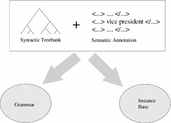
We distinguish two stages of processing: a pre-processing stage and a runtime generation stage. In the pre-processing stage (Figure 1), the grammar is automatically derived from the semantically marked-up training set in combination with the corresponding treebank structures (Sections 3 and 4). Thus, the training set has two roles in the system: it provides the instance base and serves as a basis for the rule-based grammar.
Pre-processing in the instance-based generation system.

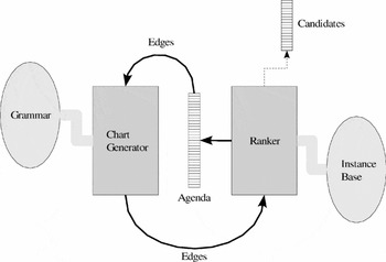
The runtime generation system (Figure 2) consists of a base generator which uses a rule-based grammar to produce candidates, potential outputs of the system. A ranker scores these candidates according to a similarity metric which measures their distance to the elements in the instance base (Section 5). The ranks are determined by the similarity to the closest instances and the highest ranked sentence is chosen as the final generation output. IBNLG uses standard chart generation techniques (Kay Reference Kay1996) in its base generator to efficiently produce generation candidates. In order to make the overgeneration-and-ranking approach to NLG feasible, we propose to interleave grammar-based construction of candidates with ranking so that the search space can be restricted early on during processing. The interleaved architecture allows us to define an efficient A*-search algorithm that prunes unpromising candidate sentences before they are fully constructed. The instance-based ranker uses information retrieval (IR) methods to rank output candidates: we represent instances and candidates as bags of n-grams and use the cosine as the distance metric. Our goal is to find the best sequence of words to be chosen as final output of the generator.
Architecture of the instance-based generator (at runtime).

The set of generation candidates forms a subset of the chart edges in that they comprise all edges of syntactic category S. The particular advantage of a bottom-up generation algorithm is that it allows a surface-based ranker to score edges as soon as they are built. The details of the base generator are generally not crucial for instance-based ranking, i.e. determining the rank order. In contrast, the induced grammar (Section 4) is important since it defines the space of possible output candidates.
To give an example of the inputs and outputs of IBNLG, consider the following corpus text:
(1) Carl E. Pfeiffer, chief executive officer, was named to the additional post of chairman of this specialty-metals manufacturing concern. (wsj_0368)
After marking up the text, the following generation input can be extracted (the semantic markup scheme is detailed in Section 3.1):
(2)

By means of rules automatically extracted from the parse trees in the annotated treebank (Section 4), the generator produces the following candidates, amongst others:
- (3)
a. Carl E. Pfeiffer, chief executive officer of this specialty-metals manufacturing concern, assumed the additional post of chairman. (cos=1.0, nn=wsj_0512)
b. Carl E. Pfeiffer, chief executive officer has been named chairman, a additional post at the specialty-metals manufacturing concern. (cos=0.75, nn=wsj_0740)
c. Carl E. Pfeiffer was named to posts which had been additional of chairman. (cos=0.47, nn=wsj_0195)
d. Carl E. Pfeiffer was named chairman, the additional job. (cos=0.28, nn=wsj_1290)
The similarity scores and nearest neighbours (‘nn’) are shown in brackets. The nearest neighbour for the highest scoring candidate (3a) is the following:
(4) Charles D. Way, president of this restaurant operator, assumed the additional post of chief executive officer. (wsj_0512)
In this case, the generator was lucky to find an instance that has a perfect match with a candidate. Of the lower scoring candidates, (3c) and (3d) are actually not produced in full by IBNLG because they are pruned early (the examples have been obtained by a less efficient search strategy, but are in the search space).
3 Corpus and semantic annotation
In the Wall Street Journal, texts such as (1) are usually preceded by a headline containing the name and location of the company in question. We identified 144 such texts in the Penn Treebank (104 were used for training, 40 for testing) and manually added semantic markup. The choice of annotation scheme is influenced by considerations of the generation task on the one hand, and ease of annotation on the other. As a general design guideline, we only make distinctions (introduce tags) if this is required by the corpus and task, i.e. we test if all word sequences marked with a given tag can be substituted for each other. We follow the idea of ‘flat’ (or ‘non-hierarchical’) input structures since these can increase the paraphrasing power of the generator (Kay Reference Kay1996; Nicolov, Mellish and Richie Reference Nicolov, Mellish and Richie1996; Shemtov Reference Shemtov1998). However, IBNLG does not crucially depend on a specific input representation – the issue is only relevant for the workings of the base generator. Furthermore, we would like to point out that the focus of this paper is less on annotation and more on instance-based ranking (Sections 5 and 6).
With the exception of tag indices (Section 3.1.2), the semantic representations are indeed flat. In contrast, other work often uses flat representations of hierarchical structures, for example (Copestake et al. Reference Copestake, Flickinger, Pollard and Sag2005). Sentence (1) is annotated as follows:
(5) [INPERSON_FULLNAME Carl E. Pfeiffer], [INPERSON_OTHERPOST_NODET chief executive officer], was named to the [POST_DESCR_ADJ additional] post of [POST_NODET chairman] of this [COMP_DESCR specialty-metals manufacturing concern].
From the annotated sentence (5) we extract the generation input in (2) as an (unordered) set of attribute–value pairs and expect the generation system to produce a template such as (6):
(6) INPERSON_FULLNAME, INPERSON_OTHERPOST_NODET, was named to the POST_DESCR_ADJ post of POST_NODET of this COMP_DESCR.
Into template (6) the values, or ‘slot fillers’, can be inserted. Note that for content determination, a task outside the scope of this work, the input representations of the presented generator require not only the selection of attributes but also the generation of the appropriate slot fillers.
3.1 Annotation scheme
The form of tag names starts with a basic semantic category, followed by more detailed specifications. There are four basic semantic categories:
(1) POST: tags referring to the main position,
(2) INPERSON: persons occupying the main position,
(3) OUTPERSON: persons leaving the main position,
(4) COMP: company descriptions including subsidiaries.
Furthermore, there are tags pertaining to temporal and referring expressions. In the following we introduce some of the actually used tags based on these main semantic categories. In addition to the semantic information, explicit syntactic constraints may be added to the tag, for example POST_DESCR_ADJ. Syntactic constraints serve to ensure that the marked texts can be substituted for each other.Footnote 1 Due to space con straints we cannot discuss the annotation scheme in full detail. However, Section 3.2 provides an overview of the most frequent types of tags and describes the annotation scheme further. See (Varges Reference Varges2003) for a full description of the annotation scheme.
3.1.1 Definiteness
Particular issues arise from the need to handle definiteness when marking post names:
- (7)
a. . . . was named an executive vice president . . .
b. . . . was named president.
In (7a), the indefinite article is used to express that there is more than one ‘executive vice president’ at the main company. On the other hand, there is only one ‘president’ so no determiner is used in (7b).
One option would be to simply ignore the existence of determiners and mark all main positions just as POST. However, since the generator can only see the attributes of the inputs but not their values, i.e. the strings we are marking, it is not able to distinguish between different values and would thus generate ‘was named a president’, for example. Another option would be to include determiners in the string marked by POST. However, this is not possible since it would require discontinuous tags due to intervening material:
(8) . . . the 56-year old chairman of . . .
If we want to be able to mark the age information as well, we cannot mark ‘the’ and ‘chairman’ with the same tag in a non-hierarchical annotation scheme.
Our strategy to solve this problem is to mark posts narrowly, excluding any determiners, but to distinguish between tags without determiner (POST_NODET), indefinite post descriptions (POST_INDEF) and definite ones (POST_DEF). Example (8) is marked-up as follows:
(9) . . . the [INPERSON_AGE 56]-year old [INPERSON_OTHERPOST_DEF chairman] . . .
Template (10) shows three coordinated posts:
(10) . . . was named [POST_NODET president], [POST_NODET chief executive officer] and a [POST_INDEF director] . . .
The template records that the indefinite post is the last one in such a template. The above-mentioned POST tags expect singular nouns as slot fillers. There is also a POST_PLURAL tag (example 11 below).
3.1.2 Tag indices
The annotation scheme described so far does not account for cases where a distinction between different tags of the same type is necessary. Typical cases involve several previous posts that are located at different companies and multiple occurrences of tags when there is more than one incoming person. To distinguish these, we introduce the notion of tag indices, an additional means of representation that allows one to attach indices to pairs of tags. This adds some hierarchical structure to the otherwise flat annotation scheme.
Our general goal is to minimize the use of hierarchical structure and rather prefer more specific tags. For example, AGE always refers to a specific person and can thus be labelled INPERSON_AGE without having to introduce an index (unless several incoming persons are involved). Similarly, recursive subsidiaries do not require indices. On the other hand, a POST may belong to several persons, e.g. one incoming and one outgoing. We thus do not make the tag more specific. We concede that this does involve some manual design choices. In the extreme, one could introduce counters as part of tag names and avoid the use of indices altogether. However, this seems overly specific and motivates the introduction of tag indices. These are appended to the tag name:
(11) [INPERSON_FULLNAME+i1 Anton Amon] and [INPERSON_FULLNAME+i2 George Gourlay] were elected [POST_PLURAL+i1+i2 vice presidents] of this [COMP-_DESCR soft-drink company].
(12) [INPERSON_FULLNAME+i2+i5 Sheldon B. Lubar],[INPERSON_OTHERPOST-_NODET-+i1+i2 chairman]of[INPERSON_OTHERCOMP+i1 Lubar & Co.], and [INPERSON-_FULLNAME-+i4+i6 John L. Murray], [INPERSON-_OTHERPOST-_NODET-+i3+i4 chairman] of [INPERSON-_OTHERCOMP+i3 Universal Foods Corp.], were elected to the [POST_-BOARD+i5+i6 board] of this [COMP_DESCR engine maker].
In (11) it is shown a relatively simple case of two persons assuming the same type of post. In (12) there are two persons with their respective OTHERPOSTs and OTHERCOMPs. Moreover, both persons were elected to the same board. We therefore also need to co-index the incoming persons with the main post. At runtime, the generator needs to make sure that any indices provided with the tags as generation input are compatible with the co-indexing of the annotation. This is done by passing indices along the context-free backbone of the grammar rules and checking their compatibility when they meet.
3.2 Frequency distribution of tags
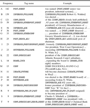
Seventy-one different tags are used to annotate the corpus of 144 sentences. They exhibit a Zipfian distribution with relatively few high-frequency tags and many low-frequency ones. The most frequent tag occurs 142 times and there are 23 singletons. The perplexity of the annotated corpus (replacing tagged sequences by labels as presented to the ranker; see Section 5) under a bigram model is 7.60. Thus, the data is relatively formulaic at the annotation level, as can be expected for domain specific news text. Crucially however, only 7% of semantic tag sets, i.e. possible inputs to the generator, occur repeatedly. Thus, pure template generation is not a viable option for realizing 93% of semantic inputs.
Table 1 shows a list of the 20 most frequent tags and gives some examples. Examples (B) and (J) show how incoming and outgoing people are labelled. The age of the incoming and outgoing person is marked by INPERSON_AGE (E) and OUTPERSON_AGE (P), respectively. The person assuming a position can have other positions in the same or other companies (D,G,S). These are distinguished from previous posts (I,Q). The COMP_DESCR tag (C) marks descriptions of the main company or organization, including nouns such as ‘company’ or ‘concern’. POST_DESCR_ADJ (H) provides additional information about the main post. The post assumed or left often is not with the main company mentioned in the headline but with a subsidiary. The proper name of a subsidiary is marked by COMP_SUBSIDIARY (K). Tag names can be assembled recursively. For example, the subsidiary of a subsidiary is labelled COMP_SUBSIDIARY_SUBSIDIARY (not shown). BOARD_INCR (L) specifies a change in the number of board members. There is a designated tag for a company's board: using the POST_BOARD tag (O) rather than other POST tags prevents the generator from producing ‘was elected to the president of’ or ‘was named a board’, for example.
The most frequent tags in the collected corpus

Verbs describing incoming events are not tagged, i.e. they are part of the template to be produced by the generator. However, in the case of outgoing events the verb can express the reason for leaving a post. It needs to be tagged if we want to avoid tying the surrounding tags to the particular reasons for leaving a post.
As (R) exemplifies, the purpose or reason for leaving a post is marked by OUTPERSON_PRP_VP plus a time suffix, where PRP stands for ‘purpose and reason’ (Santorini Reference Santorini1990). The time suffix is needed to distinguish verbs in their respective tenses. For example, INDATE_FUTURE (N) indicates that a post is occupied at a future date. Since ‘will become’ is part of the template, it will be generated by the system. This in turn requires the filler of the INDATE_FUTURE tag to name a future date.
Although generating referring expressions is not the focus of this work, we need to deal with those referring expressions that occur in the collected corpus. We see referring expressions as part of the template, i.e. we leave them unmarked. This assumes that the generator uses templates containing the referring expressions only in the right contexts. Since we are generating the first sentences of the Who's News articles, the only textual context available is the headline of the articles. Example (M) shows how we label the headlines if they are available. The demonstrative pronoun ‘this’ is the most frequent form of reference. In most cases, it is used to refer to the main company, followed by the tag COMP_DESCR (C). All occurrences of the possessive marker 's refer to a directly preceding COMP_DESCR tag, and therefore to the main company (see the example phrase of T).
4 Automatic generation grammar induction
We use the syntactic treebank in combination with the additional semantic markup to automatically produce a generation grammar that maps input semantics to surface forms. This is done by taking a set of semantic tags – and optionally tag indices – as input and generating initial phrases that can be combined into larger ones using standard chart generation techniques.
The basic idea is to identify portions of the tree structure around the semantic tags and allow these subtrees to be generated whenever the respective tag is available in the input (Section 4.2). At the next step, we identify rules that combine several phrases. This is done by a recursive bottom-up walk through the treebank structure (Section 4.3). The result of this process is the context-free backbone of a phrase-based generation grammar, which is used to automatically build the generator (Section 4.4). In the following, we describe each of these stages.
4.1 Merging annotation and treebank
The semantic markup can either be applied directly to the treebank, or, as we have done in this work, annotated sentences and treebank need to be merged. Figure 3 shows the well-known first sentence of the Penn treebank II, which happens to be part of our domain corpus, after it has been merged with the semantic annotation. There are four tags that have been applied as ‘narrowly’ as possible. In general, only constituents should be marked up. In Figure 3 all tags except POST_INDEF fully cover either a constituent or a terminal symbol. In cases like POST_INDEF we take the syntactic category of the rightmost element inside the tag to be the category of the tag, i.e. NN in this case. Furthermore, a tagged area might affect only a substring of a Penn treebank word: ‘(JJ 54-year-old)’ where only ‘54’ can be expected as generation input. If this is the case, a pre-terminal symbol is added to the syntactic structure so that the markup corresponds to a word: ‘(CD 54)(JJ -year-old)’.
Treebank merged with markup.

4.2 Input rule identification
The next step is to identify portions of the tree that can be generated by individual input tags. Starting from the tags added to the syntactic tree, we identify maximal subtrees that only dominate their individual tag but no other tags. To this end, we recursively extend ‘rule areas’ (subtrees) from input tags outwards, and stop extending areas when they are about to overlap with others. We only keep the mother nodes of the tree fragments, and ignore any internal structure. Furthermore, we omit any treebank traces. To restrict rule combinations in a semantically oriented manner, we introduce new category labels for mother nodes of phrases. These consist of the syntactic category obtained from the treebank plus the semantic tag of its leftmost daughter. As a result, the semantic information about phrases is percolated upwards to higher-level constituents. We extract four input rules for the four tags added to the syntactic tree in Figure 3:
(13) NP-INPERSON_FULLNAME → INPERSON_FULLNAME
(14) ADJP-INPERSON_AGE → INPERSON_AGE years old
(15) PP-POST_INDEF → as a POST_INDEF
(16) NP-INDATE_FUTURE → INDATE_FUTURE
Using a bottom-up grammar interpreter, rule (15), for example, can be used to match a POST_INDEF tag of the generation input and generate the phrase ‘as a POST_INDEF’ with category PP-POST_INDEF. Then the tag can be replaced by its filler to obtain ‘as a non-executive director’, for example.
4.3 Phrasal rule identification
Input rules alone do not cover the entire parse tree up to the root node. Moreover, in our example the verb remains outside the reach of the input rule areas and therefore cannot be generated yet. Thus, at the next step we introduce phrasal rules. Initially, phrasal rules are identified with input rule subtrees. These are then recursively extended – overlaps allowed – until the entire sentence structure is covered by a single rule.
The algorithm considers the entire tree structure in parallel and always tries to extend ‘rule areas’ around the most embedded nodes before considering higher level ones. Crucially, whenever two phrasal rule areas meet at the same level, we introduce a new phrasal rule area. For example, working our way backwards through the tree structure in Figure 3, we wrap the input rule categories PP-POST_INDEF' and NP-INDATE_FUTURE into a new phrasal rule area. This area can be extended up to the top-most VP, incorporating the surface words ‘will join the board’. Similarly, input rule category NP-INPERSON_FULLNAME can be combined with ADJP-INPERSON_AGE and two commas into the top-most NP (we remove the SBJ marker). At this point we have an NP and a VP at the same level of embedding, and we introduce a new phrasal rule with category Sup to combine these, also incorporating the final full stop. We use the new category Sup rather than S as the top-level sentence label to distinguish it from subordinate sentences, i.e. the generator uses Sup as its goal category. Three phrasal rules are generated from the tree in Figure 3:
(17) Sup-INPERSON_FULLNAME → NP-INPERSON_FULLNAME VP-POST_INDEF.
(18) NP-INPERSON_FULLNAME → NP-INPERSON_FULLNAME ,ADJP-INPERSON_AGE ,
(19) VP-POST_INDEF → will join the board PP-POST_INDEF NP-INDATE_FUTURE
Overall, the grammar extraction algorithm produces 1624 input and phrasal rule tokens for the 144 annotated treebank sentences, 896 of them input rules and 728 phrasal rules. By removing duplicate rules, the size of the grammar is reduced to 476 rule types overall (181 input rules and 295 phrasal rules). Again, there is a small number of high-frequency rules and a large number of singletons.
A closer look at the grammar rules reveals that 78.5% of the phrasal rules introduce additional lexical material, i.e. most phrasal rules are ‘lexicalized’ in this sense. Furthermore, most phrasal rules are binary branching (89%), some are ternary (10%) and 1% have four daughter nodes. Of the input rules, which are unary by definition (w.r.t. the number of tags on the rule right-hand side), 49% introduce additional words or punctuation.
4.4 Chart generator
In the final step of constructing the base generator, the context-free rules are converted into productions in a production system which organizes them into a Rete network (Forgy Reference Forgy1982). The Rete-based generator basically works like a standard bottom-up chart algorithm except that active edges (partially activated productions) are not part of the chart but rather part of the Rete network (as instantiations attached to the network). Compared to standard chart algorithms, Rete networks have the advantage of avoiding repeated matches when rules have some preconditions in common, i.e. they provide not just indexing but also efficient matching. This is particularly useful when large numbers of rules are derived automatically. (See (Varges Reference Varges2003) for more details.)
We do not employ any packing mechanism such as word lattices or forest structures (Langkilde Reference Langkilde2000). This is possible due to the interleaved architecture that makes it unnecessary to exhaustively generate the set of output candidates in the first place.
An example of a simplified chart edge is shown below:
(20)
Edges are labelled by their syntactic-semantic category (VP-POST in this example) and contain slots for the phonological string and for further information: a terms slot which represents the edge content to the ranker, a consumes slot which contains references to the semantics covered by the edge, a coidx slot containing the set of tag indices for this edge, and an instance slot containing pointers to the instances base (Section 5).
4.5 The need for ranking
The base generator produces large numbers of candidates depending on the size of the input and the individual tags involved. For example, inputs of size 6 typically yield about 10,000 candidates. The need for ranking arises from the fact that many candidates are ungrammatical, unintelligible or at least non-fluent. We expect the ranker to identify the ‘good’ candidates among the many ‘bad’ ones such as these:
- (21)
a. James L. Pate , 54 , , this oil concern 's , was elected a director .
b. James L. Pate , from this oil concern , , 54 years old , was elected a director .
- (22)
a. Scott C. Smith , formerly former chief financial officer was elected senior vice president at the media concern .
b. Scott C. Smith , formerly vice president, finance, , , formerly chief financial officer , was elected senior vice president at the media concern .
- (23)
a. from this metals and industrial materials maker said its board elected Michael Henderson of chairman .
b. Michael Henderson , group chief executive , This metals and industrial materials maker , 51 , was appointed chairman , effective in May , succeeding Ian Butler .
These candidates contain intelligible pieces since the automatically constructed grammar is phrase-based, i.e. many grammar rules generate several words at once. Furthermore, the slot fillers also often contain several words. As a consequence, bad candidates typically combine phrases in the wrong order but they do not exhibit random permutations of the words available to the grammar.
5 Instance-based ranking
Devising an instance-based ranking algorithm requires one to define a term representation scheme for the instances and a weighting scheme for these terms. We employ bag-of-ngram models that are similar to the bag-of-word models used in IR. Training set instances are represented as bags of terms of the form Ii = {wi ,1,. . ., wi,n} where wi,j is the weight of term j in instance i. The term representations contain the semantic tags we applied to the domain corpus and the words outside tagged areas but not the fillers. For example, in a bigram model, the marked-up string was elected a [POST president] is represented as a document vector with weighted terms {‘was elected’,‘elected a’,‘a POST’}. Punctuation marks are treated like words and result in separate tokens in the instance representation. At run-time, the ranker obtains term representations of the edge contents that potentially match these instance representations. The standard definition of the cosine distance, in our case between a candidate sentence and an instance, is
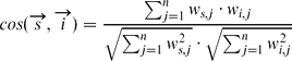
where ws,j is the weight of term j in candidate sentence s and wi,j the weight of term j in instance i. We need normalization since otherwise ever more non-matching words could be added to an edge of the chart generator without penalties. The instance-based generation system needs to compute the cosine between different edge vectors with respect to different instance vectors and compare the results. We therefore need to make the assumption that cosine scores of different origin are actually comparable. This does not seem to be an unreasonable assumption given that the cosine is often used in document clustering (Salton and McGill Reference Salton, McGill, Jones and Willett1983), for example.
We weigh terms by the well-known tf · idf term weighting scheme that assigns highest weights to terms that occur frequently (term frequency tf-component) in few instances (inverse document frequency idf-component). In contrast to IR, which mostly deals with larger texts, the ranking task for sentence generation considers relatively short sequences of words. Thus, in sentence generation tf is less important than idf since instances and edges contain relatively few terms. Furthermore, we need to devise a weighting scheme for unknown terms, i.e. edge terms generated by the grammar that are not found in the training data. Their tf component will be the count of that term in the current edge but the problem is how idf should be determined. A weight of 0 would allow the system to use non-matching terms without penalty. A weight that is too large would stifle ‘creativity’. We assign unknown terms a document frequency of 1, i.e. we pretend that it has occurred in a single instance. (This is similar to Laplace smoothing, also known as Add-one smoothing – however, in the experiments we did not add 1 to all document frequency counts.)
5.1 The search problem
Our goal is to find the candidate sentence s generated by grammar G that has the highest similarity score w.r.t. some instance i in instance base B. In principle, we need to iterate over the entire instance base for any given sentence. Given some input In, grammar G produces a potentially large number of candidate sentences. Since the instance base may be large as well, both s and i can be chosen from large sets to find the globally best cosine score cos_max_global:

where CG,In is the set of candidate sentences generated by grammar G for input In. Both s and i are variable and we are interested in finding the pair of s and i whose cosine similarity is maximal. We distinguish cos_max_global from the best cosine score for a given candidate sentence, ranging only over the instances of the instance base:

We assume that we cannot just enumerate all possible sentences for some meaning input. On the other hand, due to the interleaved architecture we do not have to wait for the grammar interpreter to produce entire sentences. We have access to all new edges being produced, including shorter ones that do not yet constitute sentences. The question is how to use this possibility of interaction.
One option is to score all new edges enew and use the highest score of enew to determine the ordering of edges on the agenda. This should give priority to longer edges that closely resemble some instance. Unfortunately, it turns out that this is not a very efficient way of ordering edges on the agenda (Section 6.1).
5.2 The basic idea: expectation-based search
Rather than matching each edge against the entire instance base, our goal is to incrementally restrict the number of instances used in similarity computations. Starting with the entire instance base for initial edges, we restrict the number of instances as edges are combined. Edges can be dropped (i.e. removed from the agenda) if there are no instances left to consider.
The key problem is to identify a property that allows us to restrict the instance base incrementally. We observe that the maximal cosine score of an edge e, cos_max_local(e, B), can increase as well as decrease when it is combined with other edges, depending on whether or not the newly added terms match the instance terms. Thus, cos_max_local(e, B) does not exhibit a monotonic behaviour that could be exploited.
We can, however, define the notion of the expectation of an edge e w.r.t an instance i which is monotonically decreasing (Section 5.3.2). This is the potentially best similarity score an edge would have with respect to a specific instance if all missing matching words were added to it:

where we,jextra is the weight of any additional occurrences of term j in e, on top of the number occurring in i. Thus, definition 4 reflects the fact that the expectation is computed under the assumption that edge e will contain (at least) all instance terms: it reuses the sum-squared instance weights (also required in the numerator and on the right of the denominator). These can be pre-computed for efficiency.
As a basic example involving just one edge e and one instance i, assume e is represented by terms a and d and i by a, b and c. Matching e against i results in one matching edge term and one mismatch. The best possible similarity score for e would be achieved by extending e by b and c to yield a,b,c,d. Actual further combinations of e can never improve upon this potentially best score as any added edge can only contribute matches (which have been assumed already) or mismatches (in which case the new expectation is lower than the previous one). Note that the expectation, in contrast to the cosine, is asymmetric since the expectation of a candidate bag is always computed with respect to a reference bag. Using the notation exp(bagcand, bagref) for the expectation, then exp(bag 1, bag 2) ≠ exp(bag 2, bag 1).
5.3 Overall search algorithm
For each new edge produced by the base generator (Section 4.4), expectations are computed and compared to the similarity score of the best candidate sentence produced up to that point. Exploiting the monotonicity of the expectation, one can omit computing the expectation for instances with which component edges of the new edge already had an expectation lower than the best candidate's score. Thus, information about the instances considered for the component edges help avoid unnecessary similarity computations for the combined edge. The similarity score of the current best candidate serves as a threshold for the remaining edges. This is similar to A*-search (Section 5.3.6): the presented ranking algorithm is admissible since it finds a single (or all) globally best solutions (if any exist).
Note that an edge has several expectations w.r.t. different instances. Thus, a new edge may use a different nearest neighbour to obtain its best expectation than its component edges. However, this new best expectation is still guaranteed to be lower or equal than the previous one.
5.3.1 Example of expectation-based ranking
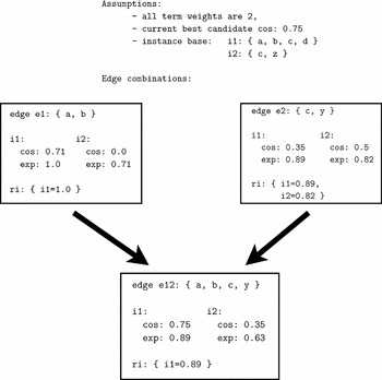
Figure 4 shows the concatenation of two edges e1 and e2 into e12 and gives cosine scores and expectations with respect to two instances i1 and i2. For example, the cosine w.r.t. instance i1 increases from 0.35 to 0.75 as e2 is combined with e1 into e12. This is because e1 contributes two matching terms (a,b). On the other hand, moving from e2 to e12, the cosine decreases from 0.5 to 0.35 w.r.t. instance i2 because e1 adds two non-matching terms (a,b). This exemplifies that the cosine is not monotonically changing in one direction.
Example of expectation-based search: edges e1, e2 combined into e12.

In contrast, the expectation is monotonically decreasing: it decreases from 1.0 for e1 w.r.t. i1 to 0.89 for e12 since e2 adds a non-matching term (y). On the other hand, viewed from e2, which has an expectation of 0.89 with regard to i1, the expectation stays the same when moving to e12. This is because the expectation has assumed the presence of the matching terms of e1 already.
For each chart edge e we define the notion of relevant instances rie. This is the table of all instances i for which the edge has an expectation higher (or equal) than the score of the current best candidate. This table indicates which expectations actually need to be computed by the ranker.
Assuming a current best candidate cosine of 0.75 and knowing that e1 has an expectation of only 0.71 w.r.t. i2, we can immediately conclude that any combination of e1 will never produce a better candidate than the one obtained already. We therefore exclude i2 from the relevant instance table of the combined edge, ri e12. (The actual expectation of 0.63 of e12 confirms this.) Thus, only exp(e12, i1) needs to be computed in this and any future edge combinations involving e12.
Note that although the resulting expectation of 0.89 remains unchanged compared to the one for e2, the expectation of a combined edge can be lower than any one of the component expectations, as exp(e12, i2) = 0.63 shows. Since most grammar rules introduce additional words (Section 4.3), further mismatches that lower the resulting expectation are likely.
In the following, we discuss the crucial monotonicity assumption (Section 5.3.2), detail the ranking algorithm (Section 5.3.3), extend it to (true) n-best search (Section 5.3.4) and introduce an additional (safe) pruning technique (Section 5.3.5).
5.3.2 Monotonicity of the expectation
The expectation of an initially empty edge e with respect to some instance i is 1 since e does not contain any non-matching terms: exp(eempty, i) = 1. The grammar rules, driven by the input, add more and more terms to e. For each term t that is added, one of two cases can arise:
(1) t does not occur in i. This decreases the cosine score as well as the expectation since it only increases the denominator of the cosine.
(2) t occurs in i:
(2.1) If t has not been present in e before, the expectation does not change since it already assumes that all correct words have been added. On the other hand, the cosine score increases.
(2.2) If t occurs in e already, we have to consider the case of the tf-component in the edge term weights. If the number of occurrences of t in e is lower or equal than its number in i (tft,e ≤ tft,i), the expectation still remains unchanged. However, if tft,e > tft,i, e may be able to neutralize the effect of its non-matching terms by repeating correct terms. Therefore, we impose an upper bound on tft,e in the numerator (but not the denominator) of the cosine and restrict it to at most tft,i. As a result, exceeding correct terms in e can only lead to an increase of the denominator and will decrease the cosine score. This guarantees that the expectation remains the upper bound of the cosine even if tft,e > tft,i).
The monotonicity of the expectation also has implications for the rule-based component: edges must always be extended monotonically. Words, and the term representations derived from them, are not allowed to be changed or removed. However, this is a standard assumption of many grammar formalisms.
5.3.3 Ranking algorithm
Each edge e is associated with its relevant instances rie (Section 5.3.1). Each i in rie is paired with an expectation w.r.t. e: rie = {i 1: exp(e, i 1),. . ., in: exp(e,in)}.
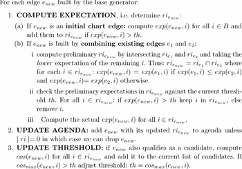
We define threshold th as the cosine score of the best candidate available at any time during processing. As long as no candidate has been produced, we assume a threshold of 0 to allow all instances to be considered. For each enew) built by a grammar rule, the ranker performs the steps outlined in Figure 5.
Sketch instance-based ranking algorithm.

First, the expectation of enew is computed. We distinguish between initial chart edges and new edges built by combining existing edges. Initial edges express individual chunks of the semantic input as built by input rules (Section 4.2). Their relevant instance table contains expectations for the entire instance base (step 1.a).
The combination of edges is performed in three steps (1.b). The first step (1.b.i) is a cheap initial approximation of rienew that reuses the already known expectations of the component edges. Taking the lower expectation is justified because the resulting edge will contain terms of both e 1 and e 2 and because of the downward monotonicity of their respective expectations. In step (1.b.ii) the resulting expectations are checked against the threshold. Instances with an expectation below th are removed from rienew. This step incrementally constrains the number of relevant instances that need to be considered in the next step. Computing the actual expectation (step 1.b.iii) involves cycling over ordered lists of term indices for instance and edge ‘in parallel’ until the end of one list is reached. Since most grammar rules introduce new surface words (Section 4.3), one needs to compute a new expectation from scratch rather than trying to reuse the expectations of the subedges in some form.
Updating the agenda (step 2) only happens if the edge is not dropped due to low expectations. Dropping edges is desirable since it leads to less edge combinations in the chart. The actual cosine score only needs to be computed when the edge is considered a candidate (step 3). However, in practice there is no big difference between calculating the cosine similarity and calculating the expectation, and both are computed together.
The performance of the expectation-based algorithm depends on how quickly a good candidate can be constructed since this sets the threshold for the remaining edges. If no candidate is available at all, no pruning takes place and the algorithm reverts to exhaustive search. However, this seems to be a rather rare case in practice (see Section 6).
5.3.4 Finding all best solutions and n-best search
The threshold can be made non-strict so that no pruning takes place for edge expectations equal to the current best candidate. This affects steps (1.a) and (1.b.ii) of the ranking algorithm (Figure 5) and the blocking of edges taken from the agenda (Section 5.3.5). As a result all best candidates are found if there is more than one.
In order to find the n best candidates, the search algorithm can be modified to keep the threshold as low as the score of the nth candidate in the ranked list, or at 0 as long as there are less than n candidates. This ensures that we never prune edges that may end up above the current nth candidate in the ranked candidate list. Like the normal threshold defined by the top-most candidate on the list, the n-best threshold increases dynamically as more candidates are generated. Note that with this modification, the search algorithm finds the true n-best list, not an approximation.
5.3.5 Blocking of agenda edges
In addition to the steps carried out for new edges about to be added to the agenda (Figure 5), the ranker performs the following check for all agenda edges about to be added to the chart:
(4) If expmax(eagenda) > th, add eagenda to chart. Else drop eagenda.
This check is performed because there is a possibility that the threshold has been increased while the edge was waiting on the agenda. It is a means for improving efficiency but does not alter the admissibility of the algorithm: since the expectation is non-increasing, it can be checked against the non-decreasing threshold at any point. (We note related issues in standard chart algorithms that we cannot discuss here; see Shieber, Schabes and Pereira Reference Shieber, Schabes and Pereira1995.)
5.3.6 Comparison to A*-search
Like the instance-based search algorithm presented above, the well-known A*-search algorithm is a best-first search algorithm that always considers the estimated best partial solution first; see text books such as (Russell and Norvig Reference Russell and Norvig2002), (Pearl Reference Pearl1984) or (Huang, Acero and Hon Reference Huang, Acero and Hon2001) for an overview. A* estimates the overall cost f from a starting state to a goal state via a current state by adding the known cost from the start state to the current state (g) to an estimate of the remaining distance (h):

Our algorithm does not make a distinction between the path from the start to the current state, i.e. from the empty edge to the current edge, and the estimated ‘cost’ of reaching the goal from the current edge. In other words, the expectation corresponds to f rather than h. In principle, the actual similarity score of an edge can be equated to function g, and correspondingly h = expectation-cosine. However, such a distinction is not necessary in our algorithm since the overall expectation can be straightforwardly computed from the bag-of-words representations.
The key difference between IBNLG and standard A*-search is the need to handle several scores and expectations which are derived with respect to different instances. This can be regarded as there being several heuristic functions rather than one. We basically treat the different heuristic functions as one by always considering only the best similarity score and expectation regardless of the instance with respect to which it has been computed. Thus, the presented algorithm can be seen as an extension of A*-search, with applications to NLG.
6 Evaluating the instance-based generator
We first evaluate a basic version of IBNLG w.r.t. its efficiency and search behaviour (Section 6.1). We identify the need for a parameter that influences sentence length, which leads to an improved version of IBNLG whose output is evaluated again (Section 6.2). We address scalability, introduce additional optimizations, and show how the generator switches nearest neighbours when increasing corpus size (Section 6.3). Finally, we present the results of a preliminary study involving human judgments (Section 6.4).
6.1 Basic IBNLG: efficiency of ranking algorithm
We trained the system on 100 randomly chosen sentences and tested it on 40 sentences.Footnote 2 The first experiment used bigram term representations and tf.idf term weighting. We employed four different search methods: the novel expectation-based ranking algorithm described in Section 5, a variation that uses the cosine to determine the agenda ordering, and pure depth-first and breadth-first search. The first two use the expectation to prune similarity computations. It is not necessary to define an explicit stopping criterion since the system is able to determine at what point during processing a best candidate has been found. Depth-first and breadth-first search have the advantage of being able to determine the agenda ordering cheaply without any similarity computation. The cosine only needs to be computed for edges that have been grown into candidates (depth-first and breadth-first search do not require it for agenda ordering). However, both depth-first and breadth-first search lead to exhaustive search if there is no pre-defined stopping criterion because no pruning takes place. Therefore, we explicitly instructed the system to halt when a first candidate with a cosine of 1.0 is found. In addition, we defined a time-out of 1 minute which was applicable to all four methods. In sum, this experiment assessed both the chart ordering strategy and the pruning strategy.
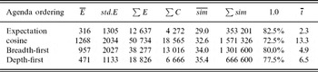
Table 2 shows the results for the 40 test set inputs. For different agenda orderings, we detail the average number of edges (E), the standard deviation of the edge counts (std. E), and the overall number of edges (∑ E); the overall number of output candidates (∑ C); the average and overall number of similarity computations, both cosine and expectation where appropriate (sim and ∑ sim); how often a candidate with similarity score 1.0 was found; and, the average time the system requires per input in seconds (t).Footnote 3
Efficiency results for test set of 40 inputs

The results show that the expectation-based ranker is the fastest and performs least overall and average similarity computations. The average number of similarity computations per edge (29) is significantly lower than the size of the instance base. Moreover, the expectation-based ranker does not exceed the time limit for any input (not shown in Table 2). Cosine-based search timed out for 12% of inputs. Breadth-first and depth-first search timed out for 5.0% and 7.5% of inputs, respectively. In case of time-outs, all counts were used up to the timeout (when the system stopped).
The cosine-based agenda seems to fare particularly badly, producing the largest number of edges and candidates and requiring the most similarity computations. It seems that using the cosine leads to prioritizing edges that also contain mismatches. In contrast, expectation-directed search basically avoids mismatches since this is the only way to decrease the expectation.
Depth-first and breadth-first search perform better than cosine-directed search. The average number of similarity computations per edge is fairly low because only a subset of the edges requires them (those that are candidates/sentences). For depth-first and breadth-first search the overall number of similarity computations is equal to the size of the instance base times the number of candidates since computing the cosine of the candidates needs to use the entire instance base. Moreover, depth-first search, despite producing less edges and candidates than breadth-first search, takes longer on average. This can be explained by the fact that depth-first search attempts more edge combinations than breadth-first search although fewer of them are successful.
6.1.1 Edge length and similarity computations
The expectation-based ranker incrementally reduces the number of instances used for similarity computations as edges are combined into larger ones. This is possible because it has access to the chart edges due to the interleaved generation architecture. We therefore expect the ranker to perform more similarity computations on shorter edges than on longer ones.
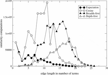
Figure 6 shows the number of overall similarity computations for the 40 test inputs w.r.t. edge length as measured by the number of terms. In general, there seems to be a tendency for the overall number of similarity computations to increase over time because more longer edges are generated by combining shorter ones. However, the maximum edge length is constrained by the size of the semantic input. Figure 6 confirms that expectation-driven search manages to reduce the number of similarity computations for longer edges. Breadth-first and depth-first search naturally score longer edges because they only rank sentences. As before, cosine-driven search fares worst, which is due to the large overall number of edges it generates.
Overall number of similarity computations (bigrams, tf.idf weights).

6.1.2 Alternative term representations
We also evaluated alternative term representations (unigrams, trigrams and mixtures) and weights (binary term weights). Detailed figures are not shown for reasons of space but the general finding is that the expectation-based algorithm is either the most efficient one or, in one case (unary terms with binary weights), close to the most efficient. Moreover, tf.idf term weighting is more efficient than binary term weighting which we explain by the increased ability to distinguish between ‘relevant’ and ‘irrelevant’ instances. Overall, the effect of the term representation scheme on efficiency is relatively limited.
6.1.3 Increasing efficiency by lowering the expectation
A crucial prerequisite in any application of the A* algorithm is the definition of an optimistic heuristic for the best possible future score. In the system described above, the expectation has been computed under the assumption that all instance terms that are still missing in an edge will eventually be added in the future. This assumption is overly optimistic: since the generator will only add new semantic tags that are in the input, it is unrealistic to expect other tags to be added. Thus, once the input tags are known, we can exclude from the computation of the expectation all instance terms that contain semantic tags that do not occur in the input. This semantic term exclusion technique effectively lowers the expectation of many edges from the start of processing, resulting in stronger pruning. As a result, the runtime of the expectation-based system is reduced significantly, for example from 2.3 to 0.5 secs for tf.idf-weighted bigram terms, and from 7.5 to 1.0 secs for binary weighted bigrams. Again, expectation-based search is more efficient than systems using other agenda ordering policies.
6.2 Improved IBNLG: fluency and completeness
We observe that the highest ranked candidates of basic IBNLG tend to be shorter than the original sentences and that they are mostly syntactically and semantically correct:
- (24)
a. output: James L. Pate was named a director of this oil concern. (cos=1.0, cov=3/6)
b. original: James L. Pate, 54-year-old executive vice president, was named a director of this oil concern, expanding the board to 14 members.
(24a) is a typical case of a short but correct candidate (‘cov’ refers to the number of realized input tags; ‘cos’ is the cosine similarity score). Example (25a) exhibits a syntactic error:
- (25)
a. output: John F. McNair III, announced that he will retire on Dec. 31 as chief executive officer and of president. (cos=0.68, cov=5/10)
b. original: First Wachovia Corp. said John F. McNair III will retire as president and chief executive officer of this regional banking company's Wachovia Corp. and Wachovia Bank & Trust Co. subsidiaries on Dec. 31.
In an experiment with trigram term representations, the candidates expressed only 55% of the input tags on average. Only 7.7% were complete. In a mixed n-gram experiment, 56% of the input tags were expressed and 10% of the candidates were complete. The average sentence length of the 40 best candidates in the trigram experiment was 13.2 words and 13.9 in the mixed n-gram experiment, in contrast to 21.9 words of the original candidates. The average template length (which replaces filler words by tags and keeps punctuation outside tags as separate tokens) was 9.1 tokens for the best candidates versus 16.3 for the original annotated sentences. Furthermore, there does not seem to be much variation in the generator output. This is reflected in the low number of support instances used to score the output candidates: 11 different nearest neighbours were used for the 40 test set inputs. In principle, the ranker could have chosen 40 different nearest neighbours from the instance base. Furthermore, only 44 different support rules were used to construct the candidates out of 384 rules specified in the grammar.
The low number of support instances points towards an explanation for the lack of completeness. Although the grammar is able to flexibly combine input tags in various ways, the instance-based ranker tends to prefer candidates conveying subsets of the input semantics that have been expressed by some training set instance. This tendency is furthered by the A*-search algorithm which uses short candidate sentences that have a high cosine score to prune away longer but lower scoring candidates. A*-search does make sure that we do not prune candidates that may turn out to be better than already obtained ones. However, once a short candidate with a similarity score of 1.0 has been found, the remaining edges are pruned away because there is no edge with an expectation larger than the threshold.
A first solution is to modify the A*-search so that it does not prune edges that have an expectation larger or equal to the cosine of the best already obtained candidate (Section 5.3.4). However, in practice this only alters the behaviour of the system in a few cases.
Another way to address the problem is to extend the definition of a ‘candidate’ from any sentence edge to also require the complete realization of the input. However, it cannot generally be assumed that the generator is always able to express the entire input semantics in one sentence. Our proposal is to use a linear combination of the similarity score and a coverage score to compute a new edge score:

The cosine between edge e and some instance i is combined with a coverage score which is computed by dividing the size of the semantics of e by the size of the input. A high value of λ places more emphasis on completeness, a low value yields candidates that more closely resemble instances. Choosing different values for λ results in candidates of different sentence lengths and input coverages. Generating complete candidate (26) below for semantic input derived from original sentence (24b) requires a λ of at least 0.2. The nearest neighbour of (26) is training set instance (27) which lacks the INPERSON_OTHERPOST_NODET tag:
(26) complete cand.: [INPERSON_FULLNAME James L Pate], [INPERSON_AGE 54] years old, [INPERSON_OTHERPOST_NODET executive vice president], was elected a [POST_INDEF director] of this [COMP_DESCR oil concern], expanding the board to [BOARD_INCR 14] members . (cos=0.95, cov=6/6)
(27) nearest neighbour: [INPERSON_FULLNAME William C. Ballard Jr.], [INPERSON_AGE 48] years old, was elected a [POST_INDEF director] of this [COMP_DESCR distilled beverages concern], expanding the board to [BOARD_INCR 11] members.
The complete candidate has a cosine score of 0.95 and has therefore previously lost out against shorter but higher scoring competitors such as (24a). The linear combination of cosine score and coverage score effectively ‘squeezes’ the missing INPERSON_OTHERPOST_NODET tag into the nearest neighbour template. (However, it should be noted that the system does not directly adapt templates; see also Section 7.3.)
One cannot know ahead of time how many different candidates there are for all values of λ, where the switching points are, or whether increasing λ would result in larger coverage. On the other hand, it seems possible to choose a ‘reasonable’ setting for λ (0.2, for example).
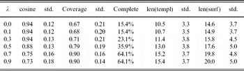
The use of a linear combination suggests that there is a trade-off between fluencyFootnote 4 and completeness in the sense that the cosine decreases as the coverage weight λ increases. This is indeed what we find. Table 3 shows average values of cosine and coverage for the test set for different values of λ. It clearly indicates that the cosine decreases as the coverage weight λ increases. Increasing λ has the desired effect of increasing the average candidate length as measured by the number words (‘len(surf)’) and by the length of the template representation (‘len(templ)’). The maximal candidate length of 20.0 words comes close to the average length of the original sentences which is 21.9 words. Maximal coverage is reached at λ = 0.7 where the average cosine score has not yet reached its minimum.
Trade-off between fluency (cosine similarity) and completeness

6.2.1 Effects of linear combination on A*-search algorithm
A linear combination of cosine and coverage score affects the computation of the expectation: we need to be optimistic about the coverage score (as we are about candidate-instance similarity) and assume that the expectation for the coverage score is always maximal (1.0). We have to make this assumption since we do not know what combinations of tags are licensed by the grammar – again a manifestation of the fundamental problem of expressibility. The combined expectation therefore is higher than the cosine alone, making it easier for edges to pass the threshold set by the combined score of already existing candidates. Despite this, the combined expectation can be used as a threshold (as the results for λ > 0.0 in Table 3 show). This extends the search space but does not lead to problems in practice except for extreme values of λ. Typical average runtimes (on a Sun Ultra 10 machine) range for λ = 0.7. For high values of λ (>0.8), the A*-search algorithm tends to search for ever larger candidates so that we need to apply a time limit (30 s). However, as in previous experiments the expectation-based agenda ordering ensures that good candidates are generated early during processing, i.e. we do not seem to miss any better candidate although the search space has not been fully explored before the time limit applies. Only in the extreme case of λ = 1.0 is there no guidance by the expectation since (combined) score and expectation are fully dominated by the coverage values.
6.3 Scalability and nearest neighbour switching
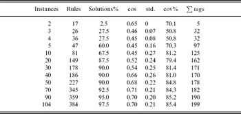
To investigate how the generation system scales with respect to the size of the grammar and the instance base, we compiled a number of sub-grammars/instance bases and tested them on the 40 test set inputs. Table 4 shows the results of experiments with these different resources, using the linear combination of similarity and coverage score (λ = 0.7). The first two columns detail the available training resources: the number of sentences used, which is equal to the number of instances (‘instances’), and the number of grammar rules automatically derived from the annotated sentences (‘rules’). Column (‘solutions’) shows for how many test set inputs it was possible to generate at least one solution. The following columns detail the average cosine scores and standard deviations of the solutions found, the coverage of the input tags of these solutions (‘cov’; this is without averaging over those inputs for which no solution was found), and the total number of tags realized by the candidates across the test set (‘∑ tags’).
Results of scalability experiments (trigram terms, tf.idf, λ = 0.7)

As Table 4 shows, five examples are sufficient to yield at least one candidate for more than half of the inputs. The largest grammar generates candidates for 39 inputs. (One input contains an unknown POST tag which makes realization with our specialized grammar impossible. Note also that in this experiment the maximum size of the training set/instance base is 104.) Not entirely surprisingly, the experiments suggest that more corpus examples will further increase the coverage of the grammar. The general tendency is an increase of the similarity score as the grammar and instance base grow larger. On the other hand, the linear combination forces the system to express more input tags so that the cosine slightly decreases for the largest training sets (while coverage still increases).
The test set provides 238 input tags. The maximal number of tags expressed by the generator is 199 for the largest grammar. This corresponds to 83.6% overall coverage of the generator.
6.3.1 The benefits of a large instance base
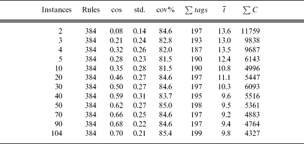
A variation of the previous scalability experiment is to keep the number of grammar rules fixed and only vary the size of the instance base. This better evaluates the effect of instance based ranking. We used the maximal number of rules, which yields candidates for 39 inputs. Table 5 shows that fluency as well as efficiency increase as the instance base grows larger. For very small instance bases, the grammar is less likely to generate a high-scoring candidate, and thus, less pruning can take place. When the instance base is large, new inputs tend to have a higher similarity to the tags expressed by some instance, and thus the generator is more likely to produce a candidate that is similar to the surface template of that instance. This in turn increases the similarity score and allows the system to prune more.
Results of scalability experiments with fixed grammar
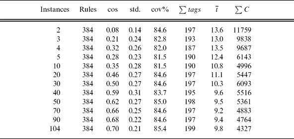
For very small instance bases, the time limit (30 s) is reached frequently. The minimum runtime is reached at an instance base of size 70 and increases slightly for the larger instance bases despite the fact that the average cosine score still grows. This may indicate that from 70 instances onwards the sheer size of the instance base begins to slow the generation system down. In that case, the technique described in Section 6.3.3 becomes relevant. (In contrast, the runtimes of the experiment with both increasing grammar and instance base (Section 6.3) were simply dominated by the increase in grammar complexity (not shown).)
6.3.2 Switching nearest neighbours
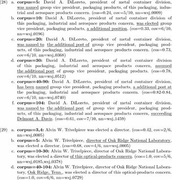
The examples in (28) and (29), Figure 7, show the ‘evolution’ of best candidates as the training set increases (settings: trigram terms, tf.idf, λ = 0.7). Preceding the candidates we indicate the size of the corpus resources that have been used. Generally, the coverage of the candidate increases with the size of the corpus. In (28), the ordering of the information as well as the main verb changes at the different stages if this is necessary to obtain a higher similarity score. These changes happen even if they do not lead to increased completeness (see 28b-28e). Note that the system is not just modifying the ‘same’ candidate but actually switches between different instances/nearest neighbours (‘nn’ in Figure 7). The reordering of information becomes apparent when we look at the placement of the word ‘additional’. The ranker uses global bag-of-terms representations and, thus, reordering happens globally as well: the goal of the ranker is to optimize the overall similarity score of the entire sentence.
‘Evolution’ of candidates with growing corpus resources.

In (29), the candidates always use the same main verb although different nearest neighbours are used. The outputs in (29c,d) show that the system can move from one perfect match with a nearest neighbour to another, more complete one as more grammar rules and nearest neighbours become available. This is because the combined score of the non-complete candidates in the linear combination still increases: the combined score of (29c) is 0.88 and increases to 1.0 for (29d). Also note that an output can be equidistant to more than one nearest neighbour (29c).
6.3.3 Dynamic rule and instance selection
To address the question how IBNLG can be scaled to instance bases and automatically constructed grammars that are much larger than in the experiments described above, we developed ‘initial semantic ranking’, a technique that effectively limits the runtime requirements of the generator. It reduces the number of grammar rules and instances to the ‘semantically relevant’ ones before generation starts by computing the cosine similarity between the semantic input and the instances represented by their semantic tags only. Crucially, this adapts the generator dynamically to the input at hand. Since we do not assume any ordering of the semantic input tags, we use unigram terms to represent input and instance semantics. These unigrams are tf.idf-weighted to avoid missing rare tags. The similarity computation only involves a single cycle over the instance base. We can then use the n-best instances and the rules derived from them for all further similarity computations in the actual generation process. This effectively adds some top-down information into the bottom-up generation process in the sense that information about the goal (the input semantics) is used to restrict search.
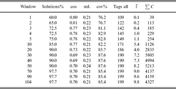
Table 6 shows results of initial semantic ranking for different window sizes, i.e. numbers of (dynamically selected) instances and associated grammar rules. Compared to the small but fixed grammars/instance bases in the first scalability experiment (Table 4), initial semantic ranking selects more appropriate resources: it provides more solutions for the inputs for the same grammar/instance base sizes, and the candidates have higher average cosine and coverage values. As the window size (i.e. the number of best sentences) increases, the results for both sets of experiments begin to look more similar, which is due to the larger overlap between the resources. As before, increasing the number of solutions can bring the average cosine and coverage scores down. A window size of 70 is sufficient to obtain the best possible results.
Results of initial semantic ranking (trigrams, tf.idf, λ = 0.7)

The efficiency results for initial semantic ranking are encouraging: although increasing the window size leads to increased runtime requirements, the growth is modest. For example, moving from a window size of 50 to 104 examples only increases the average runtime from 8.2 to 9.8 s. A larger window can decrease the number of candidates that are generated (which peaks at a window size of 30). This is because more suitable grammar rules and instances become available which allow the generation of better candidates, and hence more pruning takes place.
6.4 Human judgments of the test set candidates
Although the similarity values and the completeness of the candidates can be measured automatically, faithfulness errors and other problems need to be observed by human judges. To this end, two people (including the first author) conducted a preliminary evaluation of the output of the generator for the test set of 40 inputs. The results in this section should be seen as a ‘sanity check’ but cannot replace a more thorough evaluation. The goal of the presented paper is to establish the technical feasibility of IBNLG and explore its computational properties, rather than to explore text quality in detail – hence a more detailed human evaluation was not carried out.
In addition to faithfulness problems, we also observed other types of errors such as fluency and syntactic problems. (In this case, the term ‘fluency’ refers to what the subjects naturally considered fluent or non-fluent.) The results in this section were obtained using a trigram instance model, which should produce most fluent text since it allows the ranker to look beyond punctuation, for example.
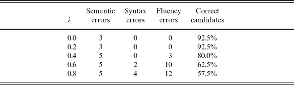
Table 7 shows the results of the manual evaluation. Semantic errors include faithfulness errors and other semantic problems. Moreover, we distinguish syntax errors from fluency errors. Examples of the error categories are shown in (28–30):
(28) Fluency: Francis D. John, 35 years old, president, was elected to . . .
(29) Syntax: This bank holding company said its board elected John W. Day.
(30) Semantics: . . . was named vice president,. . ., the new post/both new posts . . .
(28) is considered a fluency error by the two judges. In fact, no pattern like the one in (28) can be found in the corpus.Footnote 5 More fluent phrases include ‘the 35-year-old president’ and ‘35 years old, president of this . . .’, for example. (29) is a syntactic error as it violates the subcategorization frame of the ditransitive verb ‘elected’. (30) is a semantic error - the correct use of ‘both’ is beyond the capabilities of the shallow grammar.
Human judgements of best candidates (trigrams, tf.idf)
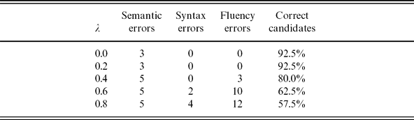
We observe an increase in the number of fluency and syntactic errors with larger values of λ (and hence, lower average cosine scores; see Table 3) – confirming our basic assumption that cosine similarity is a good indicator of fluency. The overall number of correct sentences, i.e. sentences for which no errors were found by the annotators, is maximal for λ = 0.0 and λ = 0.2 and decreases when more weight is given to completeness.
7 Comparison to related work
7.1 Overgeneration and ranking for natural language realization
The work reported in (Langkilde and Knight Reference Langkilde and Knight1998; Langkilde Reference Langkilde2000) presents hybrid sentence realizers (‘Nitrogen’ and ‘Halogen’) that use statistical n-gram and syntactic models trained on large corpora to rank output candidates that are produced by a rule-based grammar. In contrast to our approach, the Nitrogen/Halogen sentence realizer uses a two-stage pipeline without frequent interactions between candidate generator and ranker. On the other hand, both are hybrid systems that use a rule-based grammar and a corpus-based ranker. The Nitrogen/Halogen candidate generator also exhibits a bottom-up element in the way its word lattice is constructed. However, grammar organization is quite different. The Nitrogen/Halogen generator is geared toward efficient lattice/forest construction, requiring appropriate special-purpose mechanisms. In contrast, we are using a standard chart algorithm with an agenda, albeit one that is implemented in a production system. In IBNLG, the grammar is automatically constructed from a semantically annotated treebank. Nitrogen/Halogen uses a hand-built grammar and relies on the semantic formalism provided by a large, manually crafted knowledge base (Knight and Luk Reference Knight and Luk1994). The semantic input to Nitrogen/Halogen is hierarchically structured and can be defined at various levels of linguistic description. In contrast, the input to our system is a set of attribute-value pairs. Because our grammar is automatically constructed from a corpus, we know how much training material is used by the system. This is more difficult to estimate for a hand-crafted grammar.
(Bangalore and Rambow Reference Bangalore and Rambow2000) describe a realizer that uses a stochastic tree model to select TAG trees (Joshi Reference Joshi and Manaster-Ramis1987) for the words of the input structure. A hand-crafted, wide-coverage grammar is used to produce a word lattice of all possible linearizations of these trees; an n-gram model determines the word sequence with the highest probability. The system employs a hand-crafted, wide-coverage grammar – the XTAG grammar (XTAG Research Group 2001) – which required several person-years to develop. Like Halogen/Nitrogen, the system architecture is based on a pipeline without frequent interaction between grammar interpreter and ranker.
The instance-based ranking model of IBNLG is different from the above-mentioned statistical approaches. However, it is similar to statistical n-gram models in that it is purely word-based and uses n-grams extracted from the corpus sentences (which are semantically annotated in our case).
Related to the interleaved architecture of IBNLG are those approaches that integrate candidate construction with statistical ranking. (White Reference White2006) describes statistical generation with Combinatory Categorial Grammar and n-gram language models, and (Belz Reference Belz2008) describes generation with probabilistic context-free grammars. This integration makes algorithms for surface realization more similar to statistical parsing, for example by using dynamic programming and beam search to prune uninteresting edges.
7.2 Classification-based NLP
(Corston-Oliver et al. Reference Corston-Oliver, Gamon, Ringger and Moore2002; Marciniak and Strube Reference Marciniak and Strube2004; Paiva and Evans Reference Paiva and Evans2005; Mairesse and Walker Reference Mairesse and Walker2008) take generation decisions based on classifiers. In (Mairesse and Walker Reference Mairesse and Walker2008), the goal is to generate text exhibiting personality traits. For training, sentences are generated randomly, annotated by human judgments, and the classifier is trained on the trace of the generation decisions of these sentences. The actual generator uses the classifier at choice points to make deterministic decisions.
Closely related to our learning method are ‘memory-based’ approaches to NLP using classification. For example, (Daelemans, Buchholz and Veenstra Reference Daelemans, Buchholz and Veenstra1999; Sang Reference Sang2002) report on memory-based shallow parsing. Training examples are represented as feature-value vectors of fixed dimensionality labelled with a class chosen from a fixed set of labels. Following this methodology, more demanding tasks such as full-scale parsing need to be decomposed into a series of classifiers, for example into subtasks like segmentation, disambiguation and attachment resolution.
In contrast to the above-mentioned approaches, we do not frame our task as a classification problem. As a consequence, there is no need to decompose generation into a number of separate decisions. Instead, IBNLG globally optimizes its decisions by comparing bags of terms (of instances and output candidates).
7.3 Example-based Machine Translation
Example-based Machine Translation (EBMT) (Brown Reference Brown1996; Somers Reference Somers1999) also uses a learning method closely related to ours. However, there seem to be at least two major differences between IBNLG and EBMT, apart from the task which is not explicitly MT in our case. The first is the overall architecture. At least conceptually we start by opening up a space of possibilities for the ranker to choose from and then rank among the alternatives (although in practice, candidate generation and ranking are interleaved). In contrast, EBMT systems – and also the case-based realizer described in (Pan and Shaw Reference Pan and Shaw2004), for example – first search for the most similar examples and then try to adapt them, which requires specialized adaptation rules. The EBMT approach takes a direct route for arriving at a translation. The overgeneration approach takes a more indirect route: we perform the adaptation before/during the computation of the nearest neighbour. Only the initial semantic ranking technique (Section 6.3.3) performs similarity computations first.
Second, like the overgeneration approaches of statistical MT and statistical realization systems, our architecture allows us to model target language fluency. In contrast, target language fluency is typically not taken into account by the similarity metric in EBMT. Rather, EBMT systems perform similarity computations on source language strings in the first processing stage.
7.4 Grammar induction
The grammar induction method used in IBNLG (Section 4) predates two more recent approaches. (DeVault, Traum and Artstein Reference DeVault, Traum and Artstein2008) parse manually written sentences that realize the semantic representations generated by a dialogue system. Fragments of the parse trees are linked to the semantics by a set of heuristic rules, i.e. alignment is not automatic. On the other hand, these rules allow (DeVault et al. Reference DeVault, Traum and Artstein2008) to introduce additional grammatical knowledge, e.g. on agreement and subcategorization. In contrast to IBNLG, the approach does not use instance-based ranking.
(Wong and Mooney Reference Wong and Mooney2006) induce a synchronous context-free grammar (SCFG) for semantic parsing, which is inverted for generation in (Wong and Mooney Reference Wong and Mooney2007). Given a corpus of surface forms and meaning representations, word alignment models from statistical machine translation are used to align the two levels. In contrast to IBNLG, no syntactic tree structures are used. Instead, the semantic forms have hierarchical structure that can be exploited (by representing them as linearized parse trees). A further noteworthy difference to IBNLG is the ranking model: IBNLG only uses a language model and thus assumes that all candidates are equally good renderings of the meaning input (Knight and Hatzivassiloglou Reference Knight and Hatzivassiloglou1995) (with the exception of the coverage score, Section 6.2). In contrast, (Wong and Mooney Reference Wong and Mooney2007) also employ a statistical translation model to score the mapping from inputs to outputs.
7.5 Other related work
There has been substantial work on the generation of paraphrases, for example (Barzilay and Lee 2003; Cohn, Callison-Burch and Lapata Reference Cohn, Callison-Burch and Lapata2008). A major difference to our work is the expected input: paraphrase generation is a pure text-to-text application, whereas IBNLG expects marked-up pieces of text. (See also next section.)
8 Conclusions
We have developed a novel approach to natural language surface realization including lexical choice that is based on the idea of an instance-based ranking of output candidates. The approach is hybrid in that it combines a rule-based grammar with a corpus-based ranker. These interact in a novel, interleaved NLG architecture. The grammar can be interpreted as providing creativity since it can generate previously unseen sentences. Complementary, the instance-based ranker is conservative in that it prefers to reproduce events it has seen in the past. The grammar is automatically constructed from a semantically annotated corpus.
Our experiments indicate that instance-based surface realization is technically feasible and reasonably efficient, due in particular to the application of A*-search to the problem of instance-based ranking for NLG: a basic version of IBNLG is efficient but results in a preference for short output sentences (Section 6.1). This problem can be addressed by taking the semantic coverage of the chart edges into account during search (Section 6.2). Experiments regarding scalability with this improved version of IBNLG indicate that increasing the size of the instance base can improve efficiency up to a certain point, after which the size of the instance base seems to slow down the generation system (Section 6.3.1). We introduce a technique to dynamically select a subset of the instance base, which should allow IBNLG to use much larger rule and instance bases (Section 6.3.3). However, experiments with larger instance bases are required to investigate this point further. A technique that can be used in combination with all variations of IBNLG is to lower the expectation by excluding instance terms that contain semantic tags not in the input (6.1.3). The particular properties of an instance-based approach to surface realization are illustrated by observing how the system ‘switches’ nearest neighbours (Section 6.3). A preliminary human evaluation of the output of IBNLG shows that in the majority of cases the produced sentences are fluent, syntactically correct and faithful (Section 6.4).
There are also disadvantages to the presented approach: IBNLG is restricted to surface realization and lexical choice, and furthermore expects short, marked-up pieces of text as input. The level of input representation represents a compromise between the strict requirements of traditional NLG and unstructured, textual input. However, regarding the well-known question concerning the source for NLG (McDonald Reference McDonald1993), it is still unclear if this an advantage or disadvantage: can IBNLG be used in combination with an initial text analysis phase, e.g. for summarization? Can non-linguistic software components map their internal representations to the tags expected by IBNLG? Furthermore, experiments show that fluency drops if the system is forced to express more of the input, and that full coverage is not reached (Section 6.2). However, this can be regarded as the result of data sparseness problems, i.e. a larger corpus should lead to improvements.
There are many possible extensions to this work: We could use corpus annotations by several authors to bootstrap NLG systems, measure inter-annotator agreement and robustness to errors, and explore the effect of variations of the annotation scheme on paraphrasing power. Regarding grammar induction, one could add grammatical knowledge to the treebank derived generation rules, or use larger-scale syntactic language models to generalize the induced generation grammar. Regarding ranking, we could experiment with different similarity metrics, term representations (including tree structures) and weights. A particularly intriguing idea is to optimize the evaluation metric, e.g. BLEU (Papineni et al. Reference Papineni, Roukos, Ward and Zhu2002), directly. The proposed search algorithm should be applicable as long as its basic assumptions are met. In particular, it needs to be possible to construct a hypothetical optimal output text given an already constructed partial output.
Acknowledgements
This research was carried out while the authors were at the University of Edinburgh. The authors would like to thank Jon Oberlander, Chris Brew and many others for valuable discussions and inspirations. We would also like to thank the anonymous reviewers of this journal for their comments. The first author was supported by the British EPSRC, the German Academic Exchange Service (DAAD) and the University of Edinburgh. During preparation of the final version of this paper, the first author was supported by an European Commission Marie Curie Excellence Grant (ADAMACH project, contract No. 022593).