





1. Introduction and background
Canopies of protruding elements are ubiquitous in practical flows, holding significant environmental and engineering importance. Vegetation canopies are of great ecological importance to both terrestrial and aquatic ecosystems, mediating the concentration of nutrients, oxygen and carbon (Malhi Reference Malhi2002; Baldocchi Reference Baldocchi2003), as reviewed by Finnigan (Reference Finnigan2000), Belcher, Harman & Finnigan (Reference Belcher, Harman and Finnigan2012), Nepf (Reference Nepf2012a ,Reference Nepf b ) and Brunet (Reference Brunet2020). Canopies of pin-fin arrays are widely used in industrial applications for heat transfer enhancement (Ligrani, Oliveira & Blaskovich Reference Ligrani, Oliveira and Blaskovich2003; Peles et al. Reference Peles, Koşar, Mishra, Kuo and Schneider2005; Arshad et al. Reference Arshad, Ali, Ali and Manzoor2017), as summarised in Mousa, Miljkovic & Nawaz (Reference Mousa, Miljkovic and Nawaz2021). The study of canopy turbulence is also relevant to a wide range of applications, including cooling urban heat islands (Akbari & Kolokotsa Reference Akbari and Kolokotsa2016; Rahman et al. Reference Rahman, Stratopoulos, Moser-Reischl, Zölch, Häberle, Rötzer, Pretzsch and Pauleit2020), mitigating agricultural loss due to windthrow (Berry et al. Reference Berry, Sterling, Spink, Baker, Sylvester-Bradley, Mooney, Tams and Ennos2004; De Langre Reference De Langre2008), monitoring the transport of airborne pollutants (Belcher Reference Belcher2005; Escobedo, Kroeger & Wagner Reference Escobedo, Kroeger and Wagner2011; Janhäll Reference Janhäll2015) and forecasting weather (Britter & Hanna Reference Britter and Hanna2003; Blocken Reference Blocken2015). Consequently, understanding the interaction between canopies and turbulence is crucial for effectively managing such practical flows and improving the related environmental and industrial practice.
Canopy density has a direct impact on the turbulent flow within and immediately above the canopy (Nepf Reference Nepf2012a
; Brunet Reference Brunet2020; Sharma & García-Mayoral Reference Sharma and García-Mayoral2020a
,
Reference Sharma and García-Mayoralb
). Poggi et al. (Reference Poggi, Porporato, Ridolfi, Albertson and Katul2004) conducted experiments on flows over various canopy densities and identified the characteristics of different density regimes, suggesting that the flow over canopies can be broadly divided into three components. A graphical illustration of these components and their characteristic eddies for dense and sparse canopies is depicted in figure 1. The first component is the background turbulence characteristic of boundary layers – this is the component that would be present even in the absence of the canopy. The second component is the element-induced or element-coherent flow, which mainly occurs within the canopy and results from the obstruction caused by individual elements (Cava & Katul Reference Cava and Katul2008; Dupont et al. Reference Dupont, Bonnefond, Irvine, Lamaud and Brunet2011). The third component is the mixing-layer-like flow that forms due to the mean-flow inflection in the vicinity of the canopy-tip plane of a dense canopy (Raupach, Finnigan & Brunet Reference Raupach, Finnigan and Brunet1996; Finnigan Reference Finnigan2000; Finnigan, Shaw & Patton Reference Finnigan, Shaw and Patton2009). Poggi et al. (Reference Poggi, Porporato, Ridolfi, Albertson and Katul2004) emphasised that the flow behaviour near the canopy-tip plane is largely dependent on the canopy density regime, and that mixing-layer-like eddies only appear when the canopy density is high enough to induce a strong and relatively homogeneous shear layer (Raupach et al. Reference Raupach, Finnigan and Brunet1996; Sharma & García-Mayoral Reference Sharma and García-Mayoral2020b
). If we consider the eddies from the background turbulence as they penetrate into the canopy, their relative intensity and penetration depth vary depending on the canopy density (Nepf Reference Nepf2012a
; Brunet Reference Brunet2020). As illustrated in figure 1(a), dense canopies with closely packed elements effectively limit the penetration of the background turbulence, and the flow within is essentially sheltered from that above, except for a weak footprint of the mixing-layer eddies (Sharma & García-Mayoral Reference Sharma and García-Mayoral2020b
). In contrast, as depicted in figure 1(b), sparse canopies with large element spacing allow the background turbulence to penetrate relatively unhindered into the canopy. Based on this, turbulence over sparse canopies has typically been considered a simple superposition of the wall-bounded flow and the element-coherent flow, where the mean velocity profile resembles that over a smooth wall (Huang, Cassiani & Albertson Reference Huang, Cassiani and Albertson2009; Pietri et al. Reference Pietri, Petroff, Amielh and Anselmet2009; Nepf Reference Nepf2012a
). However, this argument is valid only when the drag induced by the canopy elements is negligible compared with the total drag. Recent direct numerical simulations (DNSs) have shown that even canopies with a frontal density as low as
 $\lambda _f\approx 0.01$
and spacing-to-height ratios as large as
 $s/h\approx 4$
can result in substantial element-induced drag, accounting for more than 60 % of the total drag, and that such sparse canopies mainly modulate the background turbulence through their drag on the mean velocity profile, as the mean shear sets the scale of turbulence locally at each height (Sharma & García-Mayoral Reference Sharma and García-Mayoral2020a
).
Graphical illustration of the flow regimes over (a) dense and (b) sparse canopies. The dark blue, orange and green arrows represent the background-turbulence eddies, mixing-layer-like eddies and element-coherent eddies, respectively. Adapted from Poggi et al. (Reference Poggi, Porporato, Ridolfi, Albertson and Katul2004) and Sharma (Reference Sharma2020).

Schematic representation of (a) a canopy element and (b) a layout of canopy elements. In (a),
 $A_f$
is the frontal area and
 $A_b$
is the bed area occupied by each element. In (b),
 $h$
is the element height,
 $w_x$
,
 $g_x$
and
 $s_x$
are the element width, gap and spacing (pitch) in the streamwise direction, respectively, and
 $w_z$
,
 $g_z$
and
 $s_z$
are those in the spanwise direction.

Instantaneous realisations of the
 $u'v'$
structures over and within canopies with the same number of elements per area and frontal density
 $\lambda _f\approx 0.91$
: (a) streamwise-packed canopy
 $\mathrm{C_{S27\times 108}}$
with
 $s_x^+\approx 27$
,
 $s_z^+\approx 108$
and
 $h^+\approx 110$
, and (b) spanwise-packed canopy
 $\mathrm{F_{S108\times 27}}$
with
 $s_x^+\approx 108$
,
 $s_z^+\approx 27$
and
 $h^+\approx 110$
. The structures are coloured by distance to the floor, and consist of ejections (
 $u'\lt 0, v'\gt 0$
blue to green), sweeps (
 $u'\gt 0, v'\lt 0$
red to yellow) and outward and inward interactions (
 $u'v'\gt 0$
grey to white). Cases
 $\mathrm{C_{S27\times 108}}$
and
 $\mathrm{F_{S108\times 27}}$
are fully defined in table 1.

A popular quantity to characterise canopy density is the frontal density (Nepf Reference Nepf2012a ), also known as the leaf area index in the vegetated-canopy literature (Wooding, Bradley & Marshall Reference Wooding, Bradley and Marshall1973; Kaimal & Finnigan Reference Kaimal and Finnigan1994)
 \begin{equation} \lambda _f = \frac {A_f}{A_b} = \frac {1}{A_b}\int _{0}^{h} w_z(y){\rm d}y, \end{equation}
where
 $A_f/A_b$
indicates the frontal area per unit bed area,
 $h$
is the element height and
 $w_z(y)$
is the element frontal width at each height
 $y$
, as depicted in figure 2(a). For the present prismatic canopies, the frontal density becomes
 $\lambda _f=w_z h /(s_x s_z)$
, as shown in figure 2(b), where
 $w$
indicates the element width,
 $g$
the gap between elements and
 $s$
their pitch or spacing, with the subscripts referring to the streamwise (
 $x$
) and spanwise (
 $z$
) directions. Nepf (Reference Nepf2012a
) noted that canopies are dense when
 $\lambda _f\gg 0.1$
, sparse when
 $\lambda _f\ll 0.1$
and intermediate between the two limits. Permeability and porosity (
 $\phi$
) are also popular measures of density for denser canopies and other permeable substrates, embodying the ‘accessibility’ of the fluid region (Breugem, Boersma & Uittenbogaard Reference Breugem, Boersma and Uittenbogaard2006; Lightbody & Nepf Reference Lightbody and Nepf2006; Luhar, Rominger & Nepf Reference Luhar, Rominger and Nepf2008). However, these geometric parameters only provide a notional measure of canopy density, and occasionally fail to capture how different element arrangements can result in different flow regimes. The studies by Pietri et al. (Reference Pietri, Petroff, Amielh and Anselmet2009) and Bailey & Stoll (Reference Bailey and Stoll2013) highlighted that identical density values of
 $\lambda _f$
and
 $\phi$
do not necessarily translate to similar flow penetration behaviours and may not accurately reflect the actual canopy density regime. This limitation is illustrated in figure 3, depicting structures of intense
 $u'v'$
over canopies with the same number of elements and identical
 $\lambda _f$
but different element layouts, which are discussed in full detail in § 4.1. As shown in figure 3(a), these structures penetrate more effectively into the streamwise-packed canopy compared with the spanwise-packed canopy in figure 3(b), showing that element layout, a factor not captured by
 $\lambda _f$
, can significantly influence the canopy density regime.
The frontal density
 $\lambda _f$
has been proposed as a predictor for canopy density because it is a convenient surrogate for physics-based quantities, such as the drag length
 $\ell _d$
, which characterise the impedance that the canopy exerts on the flow (Nepf Reference Nepf2012a
). The drag length
 $\ell _d$
gives a measure of how quickly the mean flow
 $U(y)$
decays below the canopy tips, and can be defined as
 $\ell _d=U^2/F_D$
using the mean velocity and surface drag
 $F_D$
at the plane of the tips. It would then be natural to expect that the differences between streamwise- and spanwise-packed layouts mentioned above could be captured by parameters such as
 $\ell _d$
since, even for the same
 $\lambda _f$
, the higher drag sheltering for streamwise-packed configurations results in a larger
 $\ell _d$
. Other length scales that can quantify the penetration of the mean flow are the shear length
 $\ell _s=U/({\rm d}U/{\rm d}y)$
measured at the tip plane, which quantifies how inflexional the
 $U(y)$
profile is, and thus the intensity of the drag acting on it (Endrikat et al. Reference Endrikat, Modesti, García-Mayoral, Hutchins and Chung2021), or the depth below the tips of the zero-plane displacement,
 $d_0$
, the depth perceived as the origin by the overlying turbulence (Chen & García-Mayoral Reference Chen and García-Mayoral2023). All these length scales, however, characterise the effect of the canopy on the penetration of the mean velocity profile, rather than of the set of fluctuating eddies that conform the overlying turbulence. This paper will propose a length scale to characterise canopy density based on the latter. For conventional canopy layouts, such as
 $x$
–
 $z$
-isotropic vegetation canopies and their regular surrogates often studied in the literature, we would expect reasonable correlation between both approaches, but possibly not for counter-examples such as those of figure 3. An assessment of the above length scales as predictors for density can be found in Appendix A. They provide a generally correct trend but with significant scatter, comparable to that produced using the purely geometric
 $\lambda _f$
.
Sharma & García-Mayoral (Reference Sharma and García-Mayoral2020a
) argued that a canopy would be sparse if the spanwise spacing between elements is
 $s_z^+\gtrsim 100$
, which is large enough to fit in the near-wall streaks of characteristic width
 $\lambda _z^+\approx 100$
(Kline et al. Reference Kline, Reynolds, Schraub and Runstadler1967; Kim, Kline & Reynolds Reference Kim, Kline and Reynolds1971). This is consistent with the observations of Poggi et al. (Reference Poggi, Porporato, Ridolfi, Albertson and Katul2004) and Huang et al. (Reference Huang, Cassiani and Albertson2009), who noted a progressive departure from smooth-wall behaviour for sparse canopies as the spacing between elements decreases. However, Sharma & García-Mayoral (Reference Sharma and García-Mayoral2020a
) investigated only sparse canopies of isotropically laid filaments, and did not consider the effects of a wider variety of geometric parameters; a spanwise spacing can be easily defined for the collocated elements of Sharma & García-Mayoral (Reference Sharma and García-Mayoral2020a
), but doing so for irregular or even staggered arrangements may be less straightforward. Canopies that are clearly sparse or clearly dense were extensively investigated in Sharma & García-Mayoral (Reference Sharma and García-Mayoral2020a
) and Sharma & García-Mayoral (Reference Sharma and García-Mayoral2020b
), but the transition from one limit to the other was not directly considered. This highlights the need for a more systematic approach to measure the extent of turbulence penetration, and to characterise canopy density. Recent studies have proposed to characterise canopy density as determined by the interchange between the relative vertical positions of the zero-plane-displacement height and the inflection in the mean velocity profile that occurs within the canopy (see e.g. Monti et al. Reference Monti, Omidyeganeh, Eckhardt and Pinelli2020, and follow-up papers). The latter inflection occurs due to the near-bed boundary layer that forms in order for the mean flow to satisfy no slip at the bed. The authors argued that this lower inflection played a key role in the flow dynamics, as it gave rise to an instability, reminiscent of Kelvin–Helmhotz, because the mean velocity profile satisfied Fjørtoft’s criterion for instability. The opposite is unfortunately the case: Fjørtoft’s criterion predicts instability for a mixing-layer type, concave-to-convex inflection, like the one at the canopy tips, and stability for convex-to-concave inflections like the one near the bed. Physically, the flow is the most unstable where the mean shear is maximum, and most stable where the shear is minimum. Furthermore, for flows in homogeneous canopies, the lower inflection can only occur when the flow is driven by a mean pressure gradient or a body force, when a Darcy-like region of uniform velocity tends to form in the canopy core, requiring a Brinkman-like boundary layer at its bottom to meet no slip at the bed. Beyond pressure gradients, inner inflections can also appear when there is a local maximum in the mean velocity profile within the canopy, which can be caused by inhomogeneities such as edge effects and differences between trunk and crown drag (see e.g. Dupont et al. Reference Dupont, Bonnefond, Irvine, Lamaud and Brunet2011, and references therein). Otherwise, when the intra-canopy flow is driven mainly by the shear exerted by the overlying flow, as in zero-pressure-gradient boundary layers, the Darcy-flow contribution is non-existent, and there is therefore no inner inflection. A different approach is therefore necessary to characterise canopy density in a common framework across the broad flow typology.
In the present study, we conduct DNSs of canopies with different layouts and element geometries. We aim to establish a metric for canopy density based on the flow dynamics to enable the quantitative diagnosis, characterisation and prediction of canopy density. For this, we quantify the extent and depth of the penetrating three-dimensional turbulence structures of intense Reynolds shear stress
 $u'v'$
(Del Alamo et al. Reference Del Alamo, Jiménez, Zandonade and Moser2006; Lozano-Durán et al. Reference Lozano-Durán, Flores and Jiménez2012). We focus on these structures because they are responsible for momentum transport and turbulence diffusion between the overlying and the canopy regions, and are ultimately responsible for the wall-normal distribution of the Reynolds stress and thus the shape of the mean velocity profile. Based on this measure, we explore the influence of the different geometric characteristics of the canopy on whether turbulence penetrates or not, and identify which are the key ones to determine canopy density. The paper is organised as follows. § 2 presents the numerical method and the different canopies simulated. § 3 introduces and discusses the metrics used to measure turbulence penetration. § 4 presents the DNS results, focusing on how different canopy parameters affect turbulence penetration. Finally, § 5 summarises the conclusions of our investigation.
2. Methodology
In this section, we briefly discuss the DNS method in § 2.1, and present the relevant parameters for the canopies simulated, with different element geometries and layouts, in § 2.2.
Schematics of the numerical channel for (a) spanwise-packed canopy
 $\mathrm{F_{S216\times 54}}$
, with streamwise spacing
 $s_x^+\approx 216$
, spanwise spacing
 $s_z^+\approx 54$
and canopy height
 $h^+\approx 110$
, all in viscous units, and (b) streamwise-packed canopy
 $\mathrm{C_{S54\times 216}}$
, with
 $s_x^+\approx 54$
,
 $s_z^+\approx 216$
and
 $h^+\approx 110$
. The channel half-height is
 $\delta$
. Details of the canopy geometries are presented in table 1. An instantaneous realisation of the streamwise velocity is shown in axis-orthogonal planes, from dark to clear
 $u^+=0$
to
 $u^+=15$
in (a) and
 $u^+=0$
to
 $u^+=19$
in (b).

2.1. Direct numerical simulations
We carry out DNS of doubly periodic closed symmetric channels with rigid filament canopies protruding from both walls. The coordinates
 $x$
,
 $y$
and
 $z$
represent the streamwise, wall-normal and spanwise directions, respectively. The filament canopies and the numerical domain studied are portrayed in figure 4, where
 $\delta =1$
is the channel half-height measured from the channel centre to the canopy-tip planes. The canopy elements extend below
 $y=0$
on the bottom wall and above
 $y=2\delta$
on the top wall. For all simulations the channel streamwise and spanwise dimensions are at least
 $L_x\times L_z=2\pi \delta \times \pi \delta$
, and up to
 $2.8\pi \delta \times 1.4\pi \delta$
. Compared with open channels, closed channels entail roughly twice as much computational cost per time step, but they also produce twice as many statistical samples. The two set-ups are essentially equivalent for the near-wall flow. They can exhibit different properties in the wake region above the logarithmic layer, where turbulence activity is significantly inhibited by the no-transpiration boundary condition in open channels, while the centre of a closed channel allows eddies to flow freely, with a closer resemblance to boundary layers. For canopy flows we have reported these wake differences in Chen & García-Mayoral (Reference Chen and García-Mayoral2023), where they were confined to the top
 $\sim$
20 % of the flow thickness, and they are examined in depth across different flows, including open and closed channels, Couette flow and boundary layers, in Luchini (Reference Luchini2018, Reference Luchini2024).
The DNS code in this study is from Sharma & García-Mayoral (Reference Sharma and García-Mayoral2020a ,Reference Sharma and García-Mayoral b ) and has been validated in Sharma (Reference Sharma2020) and Chen & García-Mayoral (Reference Chen and García-Mayoral2023). It is summarised here for reference. The numerical method resolves the three-dimensional incompressible Navier–Stokes equations,
 \begin{align} \frac {\partial \boldsymbol{u}}{\partial {t}} + \boldsymbol{u}\boldsymbol{\cdot }\boldsymbol{\nabla }\boldsymbol{u} &= -\boldsymbol{\nabla }\!{p} + \frac {1}{\textit{Re}}{\nabla} ^2\boldsymbol{u}, \end{align}
 \begin{align} \boldsymbol{\nabla }\boldsymbol{\cdot }\boldsymbol{u} &= 0, \end{align}
where
 $\boldsymbol{u}=\langle u,w,v \rangle$
is the velocity vector with components in the streamwise, spanwise and wall-normal directions, respectively,
 $p$
is the kinematic pressure and
 ${\textit{Re}}$
denotes the bulk Reynolds number
 ${\textit{Re}}=U_b\delta /\nu$
based on the bulk velocity
 $U_b$
, the channel half-height
 $\delta$
and the kinematic viscosity
 $\nu$
. The simulation is operated at a constant mean pressure gradient
 $-\partial _x P$
, with the flow rate adjusted to achieve the targeted friction Reynolds number
 ${\textit{Re}}_{\tau} =u_{\tau} \delta /\nu \approx 180-2000$
, where
 $u_{\tau} =\sqrt {\delta \,\partial _x P }$
is the reference friction velocity at the canopy-tip plane. No-slip and impermeability boundary conditions are applied at both channel walls. The rigid elements are resolved using a direct-forcing, immersed-boundary method (Mittal & Iaccarino Reference Mittal and Iaccarino2005; García-Mayoral & Jiménez 2011). In this work, variables scaled with
 $u_{\tau}$
and
 $\nu$
are termed as in inner units, denoted by superscript
 $(\boldsymbol{\cdot })^+$
, and those scaled with
 $U_b$
and
 $\delta$
are referred to as in outer units.
In the wall-normal direction, a second-order central difference scheme is applied on a staggered grid. At the channel centre, where the mean shear is the weakest, the stretched wall-normal grid has a resolution
 $\Delta y_{max}^+\approx 3.0$
when
 ${\textit{Re}}_{\tau} \approx 180$
. At higher Reynolds numbers, where dissipation occurs at larger scales (Jiménez Reference Jiménez2012),
 $\Delta y_{max}^+$
extends from 3.6 to 7.0 as
 ${\textit{Re}}_{\tau}$
increases from 360 to 2000. The finest resolution
 $\Delta y_{min}^+$
is at the floor or canopy-tip plane, wherever the mean shear is the greatest. For all cases,
 $\Delta y_{min}^+\lesssim 0.3$
is satisfied when scaled with the local, dynamically relevant friction velocity, as proposed in Sharma & García-Mayoral (Reference Sharma and García-Mayoral2018, Reference Sharma and García-Mayoral2020a
).
The discretisation in the periodic, wall-parallel directions is spectral. To balance computational cost and resolution, the numerical domain is divided into blocks with different wall-parallel resolutions (García-Mayoral & Jiménez Reference García-Mayoral and Jiménez2011). The wall blocks, containing the roughness sublayer, have a finer resolution than the block encompassing the channel centre. In the finer blocks, the grid resolution resolves not only the turbulent scales but also the canopy geometry and the element-coherent eddies, which are typically of the order of or smaller than the element width (Poggi et al. Reference Poggi, Porporato, Ridolfi, Albertson and Katul2004). Consequently, the wall-parallel grid spacings in
 $x$
and
 $z$
are smaller than
 $w_x^+$
and
 $w_z^+$
. Sharma & García-Mayoral (Reference Sharma and García-Mayoral2020b
) examined wall-parallel resolutions for dense canopies, and concluded that a marginal resolution of 9 points per spacing and 3 points per element width for a filament canopy with
 $s^+\approx 24$
,
 $w^+\approx 5$
and
 $h^+\approx 100$
could underestimate the turbulent fluctuation within the canopy, with a maximum deviation of up to 20 % observed in the wall-normal fluctuations, although this discrepancy reduced to 4 % just above the tips. In our case, the most resolution-demanding simulations are typically those with relatively thin elements or narrow gaps, where small grid spacings are required to resolve the canopy geometry or the fluid in between elements. In table 1, the canopy with thinnest filaments is
 $\mathrm{G41_{S47\times 47}}$
, with
 $w_x^+=w_z^+\approx 6$
and
 $s_x^+=s_z^+\approx 47$
, which is simulated with a resolution
 $\Delta x^+=\Delta z^+\approx 2$
. For canopy
 $\mathrm{IS2000_{G30\times 30}}$
at
 ${\textit{Re}}_{\tau} \approx 2000$
, with
 $w_x^+=w_z^+\approx 24$
and
 $s_x^+=s_z^+\approx 54$
, the resolution is also marginal at
 $\Delta x^+=6$
and
 $\Delta z^+\approx 3$
. Such marginal resolutions are applied only for the densest canopy cases, for which fluctuations within the canopy are in any event weak compared with those above, and thus higher resolutions do not change the behaviour observed. For all other canopies, a minimum of 16 points per streamwise or spanwise pitch are used. The height of the fine blocks is chosen such that the small and rapid element-coherent eddies decay naturally before approaching the coarse block at the channel centre, which has a standard smooth-wall resolution of
 $\Delta x^+\approx 8$
and
 $\Delta z^+\approx 4$
(Jiménez & Moin Reference Jiménez and Moin1991). The height above the canopy tips of the fine-resolution blocks is set to at least twice the element width for sparse canopies and twice the gap size for dense canopies, correlating with the height of the roughness sublayer (Chen & García-Mayoral Reference Chen and García-Mayoral2023). This is validated a posteriori by examining the spectral densities of turbulent fluctuations to ensure that any small-wavelength signal has already vanished well below the inter-block interface.
Simulation parameters. Here,
 $N_x$
and
 $N_z$
are the numbers of elements in the streamwise and spanwise directions, respectively;
 ${\textit{Re}}_{\tau} =\delta u_{\tau} / \nu$
is the friction Reynolds number;
 $\lambda _f$
is the frontal density;
 $s_x$
,
 $s_z$
,
 $g_x$
and
 $g_z$
are the pitch and gap in the streamwise and spanwise directions, respectively, and the element width is
 $w=s-g$
;
 $h$
is the canopy height. The ‘+’ superscript indicates viscous scaling, i.e. with the friction velocity
 $u_{\tau}$
and the kinematic viscosity
 $\nu$
. Case names with the same superscript are the same DNS.

2.2. Simulation parameters
We consider flows over canopies with rigid prismatic elements to thoroughly investigate turbulence penetration across various canopy layouts, element geometries and Reynolds numbers. We are mainly concerned with canopies fully immersed in boundary layers, so our simulations fall in the range
 $\delta /h=5$
-
 $20$
. A few cases, in intermediate-to-dense regimes with relatively small pitch, were run at
 $\delta /h \approx 3.3$
, but for these closely packed canopies the roughness layer scales with element spacing, rather than height (Chen & García-Mayoral Reference Chen and García-Mayoral2023). Under the above conditions, an overlying turbulence, self-sustained independently of the presence of the canopy, can properly develop, and whether it penetrates within the canopy or not can be discussed. We can then expect outer layer similarity to hold. In contrast, in canopies with
 $\delta /h\lesssim 2$
, typical of aquatic vegetation in shallow-submergence or emergent conditions, the whole flow is fully embedded within or directly affected by the canopy (Nepf & Vivoni Reference Nepf and Vivoni2000; Zhao & Nepf Reference Zhao and Nepf2024), and an overlying turbulence cannot be meaningfully defined. The latter are therefore out of the scope of the present work.
Figure 2 illustrates the morphology of the canopies studied, and table 1 details the relevant simulation parameters. We note that in the literature, the terms ‘spacing’ and ‘gap’ are sometimes used interchangeably, mainly in the context of canopies with thin filaments, where the element width
 $w$
is small compared with both
 $s$
and
 $g$
, so that
 $s=g+w\approx g$
(Cui, Patel & Lin Reference Cui, Patel and Lin2003; Bailey & Stoll Reference Bailey and Stoll2013). Here, we consider both thin filaments (
 $w/s\approx 0.06$
) and thick and densely packed elements (
 $w/s\approx 0.67$
). To avoid confusion, we refer to the ‘spacing’
 $s$
, the sum of the gap and element width, as the ‘pitch’ in the remainder of this work.
All canopies investigated consist of collocated prismatic elements with a square wall-parallel cross-section, with
 $w_x=w_z$
. To distinguish among different simulations, the prefix indicates the canopy characteristics, and the subscript denotes the approximate streamwise and spanwise spacing/pitch (‘S’) or gap (‘G’) in inner units. For example, case
 $\mathrm{C_{S27\times 108}}$
refers to a canopy resembling a ‘canyon’ with streamwise-packed elements, where
 $s_x^+\approx 27$
and
 $s_z^+\approx 108$
.
In table 1, the first five groups consist of canopies with identical element geometry, where
 $h^+ \approx 110$
and
 $w_x^+ = w_z^+ \approx 24$
, but with different pitches and gaps. The first group, prefixed with ‘I’, consists of isotropic canopies with equal streamwise and spanwise pitches
 $s_x^+=s_z^+$
. These isotropic canopies are from Chen & García-Mayoral (Reference Chen and García-Mayoral2023), which showed that turbulence effectively penetrates the sparse canopy
 $\mathrm{I_{S432\times 432}}$
and perceives an origin at the floor, while turbulent eddies ‘skim’ over the dense canopy
 $\mathrm{I_{S36\times 36}}$
and perceives a smooth wall at the tips. The second and third groups consist of fence-like canopies prefixed with ‘F’, with spanwise-packed elements, and canyon-like canopies prefixed with ‘C’, with streamwise-packed elements, each matching the total number of posts of isotropic canopies
 $\mathrm{I_{S54\times 54}}$
to
 $\mathrm{I_{S216\times 216}}$
and therefore the value of
 $\lambda _f$
. It will be demonstrated in § 4.1 that canopies with the same
 $\lambda _f$
can result in different turbulence penetration behaviours, depending on whether the elements are more closely distributed in the streamwise or spanwise direction. Cheer & Koehl (Reference Cheer and Koehl1987) investigated flow through biological bristles, and showed that fence-like structures can behave as a ‘paddle’ (a single solid obstacle) or a ‘rake’ (a permeable one), depending on the gap size
 $g^+$
. In the fourth group, marked by ‘Z’, we gradually reduce the number of posts in the streamwise direction
 $N_x$
from the canyon-like canopy
 $\mathrm{C_{S27\times 108}}$
, keeping all spanwise parameters (
 $N_z$
,
 $s_z^+$
and
 $g_z^+$
) fixed. Similarly, the fifth group, denoted by ‘X’, consists of canopies with different
 $N_z$
but with the same streamwise parameters. In § 4.2, with the ‘Z’ and ‘X’ groups, we investigate whether parameters in the streamwise or spanwise direction have more impact on flow penetration. To identify whether the gap or pitch matters, we study canopies with a fixed gap but different pitch (group ‘G’) or with a fixed pitch but different gap (group ‘S’) in § 4.3. The number that follows prefixes ‘G’ and ‘S’ denotes the approximate value of the fixed gap and pitch in inner units, respectively. Finally, in § 4.4, we investigate the effect of the Reynolds number using canopies with similar geometry in outer (same
 $s/\delta$
,
 $g/\delta$
and
 $h/\delta$
in group ‘OS’) or inner units (same x‘
 $s^+$
,
 $g^+$
and
 $h^+$
in group ‘IS’).
3. Measuring the penetration of turbulence into the canopy
Before we embark in the analysis of canopy density, we need to establish how to measure turbulence penetration from the overlying flow. In § 3.1, we first discuss how we identify the penetrating structures that contribute to the momentum and turbulence transport in the vicinity of the canopy-tip plane. In § 3.2, we introduce the metrics that we will use to quantify the penetration of these structures.
3.1. Identification of background structures
To investigate the penetration of the overlying background turbulence, we focus on structures of intense pointwise
 $u'v'$
(Lozano-Durán et al. Reference Lozano-Durán, Flores and Jiménez2012; Lozano-Durán & Jiménez Reference Lozano-Durán and Jiménez2014), because of their importance in momentum transport. The temporal evolution of these structures has been thoroughly studied by Lozano-Durán & Jiménez (Reference Lozano-Durán and Jiménez2014); here, we are only concerned with whether they penetrate into the canopy at any given instant, and the extent of their penetration, regardless of their dynamics, and as such we do not consider their preceding or subsequent evolution.
Just like the background, turbulence can exhibit structures of intense
 $u'v'$
, the other flow components in figure 1 can as well, including the element-coherent flow. Its structures can merge with those from the background turbulence and, if the merger is identified as a single structure, misrepresent the background turbulence as penetrating more deeply into the canopy than it actually does. To prevent this, we first filter out the element-coherent signal to isolate the background structures.
As depicted in figure 5(a), element-coherent flows typically are formed by stem-scale eddies in the wake of each obstacle. A similar pattern for stem-scale eddies is also observed in Poggi et al. (Reference Poggi, Porporato, Ridolfi, Albertson and Katul2004) and Sharma & García-Mayoral (Reference Sharma and García-Mayoral2020a ) for sparse canopies. As shown in figure 5(b), element-coherent top-shedding eddies can also form. Note that the latter are different from the canopy-scale, mixing-layer-like eddies induced by the inflectional mean profile (Raupach et al. Reference Raupach, Finnigan and Brunet1996; Nepf Reference Nepf2012a ). The element-induced, element-coherent flows shown in figure 5(a,b) are not part of the penetrating turbulence from the overlying background flow, and we therefore filter them out before measuring turbulence penetration.
Instantaneous realisations of
 $u'v'$
structures for (a,c) case
 $\mathrm{I_{S216\times 216}}$
and (b,d) case
 $\mathrm{F_{S144\times 36}}$
. Structures are coloured by distance to the floor, ejections in blue to green, sweeps in red to yellow and outward and inward interactions in grey to white. Panels show (a,b) raw flow fields and (c,d), flow fields spectrally filtered to remove the element-coherent flow.

A conventional method to obtain the background flow is through triple decomposition (Reynolds & Hussain Reference Reynolds and Hussain1972)
 \begin{align} \boldsymbol{u}(x,y,z,t) &= \boldsymbol{U}(y)+\boldsymbol{u'}(x,y,z,t), \end{align}
 \begin{align} \boldsymbol{u'}(x,y,z,t)&= \tilde {\boldsymbol{u}}(x,y,z)+\boldsymbol{u''}(x,y,z,t), \end{align}
where
 $\boldsymbol{U}$
is the mean velocity profile, and
 $\boldsymbol{u'}$
is the full temporal and spatial turbulent fluctuation. The latter can be further decomposed into a time-averaged but spatially varying component,
 $\tilde {\boldsymbol{u}}$
, and the remaining time-varying fluctuation,
 $\boldsymbol{u''}$
. The component
 $\tilde {\boldsymbol{u}}$
is often referred to as the dispersive flow (Raupach & Shaw Reference Raupach and Shaw1982) and assumed to embody the element-coherent flow. Abderrahaman-Elena, Fairhall & García-Mayoral (Reference Abderrahaman-Elena, Fairhall and García-Mayoral2019), however, suggested that the element-coherent flow is modulated in amplitude by the overlying background turbulence for roughness elements up to
 $h^+\lesssim 35$
.
In any event, as roughness size increases, wake unsteadiness intensifies, complicating the isolation of the background flow. For the present canopies, with sizes up to
 $h^+\approx 270$
and
 $w^+\approx 30$
, there is significant unsteady yet element-coherent flow, rendering (3.2) ineffective as the time-dependent element-wake flow cannot be accurately represented by the temporally averaged term
 $\tilde {\boldsymbol{u}}$
. As a practical approximation, we thus use a spectral filter to isolate the background flow, aiming to retain most of the energy of the background-turbulence wavelengths while removing the element-coherent signal. The filtering procedure is detailed in Appendix B.
The instantaneous realisations of the filtered flow field in figure 5(c,d) illustrate that both the stem-scale eddies of the sparse canopy
 $\mathrm{I_{S216\times 216}}$
and the shedding eddies of the fence-like canopy
 $\mathrm{F_{S144\times 36}}$
are removed effectively by the filter, while the background turbulent eddies remain essentially unmodified. The applied filter slightly reduces the volume of the largest structure in figure 5(c) by approximately 5 % compared with its original size in figure 5(a), which we deem acceptable. For case
 $\mathrm{F_{S144\times 36}}$
in figure 5(b,d), the large structures remain essentially unaffected by the spectral filter, as they do not significantly penetrate within the ‘fences’ in any event. These flow visualisations suggest that the applied filtering can effectively isolate the background turbulence from the element-coherent flow.
After filtering the element-induced, element-coherent flow, we define the background structures that contribute the most to the Reynolds shear stress as connected regions satisfying
 \begin{equation} |u'v'(x,y,z)|\gt H\tau _{\textit{tip}}, \end{equation}
where
 $u'v'(x,y,z)$
is the pointwise Reynolds shear stress,
 $H$
is a thresholding constant of order
 $\sim 1$
and
 $\tau _{\textit{tip}}$
is the total shear stress evaluated at the canopy-tip plane. The rigorous determination of a common value for
 $H$
across all our simulations is discussed in Appendix C. In the discretised space of the simulations, the connectivity is established between immediately neighbouring points along
 $x$
,
 $y$
or
 $z$
that satisfy (3.3), to ensure that only physically contiguous regions of high
 $|u'v'|$
are identified as a single connected structure.
3.2. Metrics for the penetration of background-turbulence structures
Once we have isolated the background turbulent structures from the full flow field, we can narrow our focus to the structures that cross the canopy-tip plane, as they embody turbulence penetration from above. Of the whole background, overlying turbulence, these are the eddies that come into contact with the canopy. In this subsection, we introduce measures for the location, span and volume of these ‘tip-plane-intersecting’ structures, which we will refer to as ‘interfacial eddies’ from here on, aiming to characterise the extent and depth of their penetration into the canopy.
Probability density function (p.d.f.) of the (a)
 $y$
, (b)
 $x$
and (c)
 $z$
distributions of interfacial eddies of intense
 $u'v'$
for canopy
 $\mathrm{I_{S216\times 216}}$
as a function of the eddy size. Here,
 $V$
is the eddy volume and
 $\delta$
the half-channel height. The solid and dotted contour lines represent statistics for the volume and the density of
 $u'v'$
, respectively, and enclose 95 % of the penetrating eddies; The 25th, 50th (centroid) and 75th percentiles are represented by the red, purple and blue lines, respectively. In the wall-parallel directions, the percentile locations are measured relative to the position of the centroid,
 $x_c$
-
 $z_c$
.

The mean location of a structure can be characterised by the centroid position of its volume
 $V$
 \begin{equation} \boldsymbol{x}_{c, vol} = \frac {\int _\varOmega \boldsymbol{x}(x,y,z) {\rm d}V}{\int _\varOmega {\rm d}V}, \end{equation}
and also by the centroid position of its
 $u'v'$
distribution
 \begin{equation} \boldsymbol{x}_{c, uv} = \frac {\int _\varOmega u'v'(x,y,z)\,\boldsymbol{x}(x,y,z) {\rm d}V}{\int _\varOmega u'v'(x,y,z) {\rm d}V}, \end{equation}
where
 $\boldsymbol{x}$
is the pointwise position vector for all contiguous points within the volume of the structure,
 $\varOmega$
. The spatial extent of a structure can be characterised by its maximum (
 $\boldsymbol{x}_{max}$
) and minimum (
 $\boldsymbol{x}_{min}$
) positions in
 $x, y$
and
 $z$
. However, we typically observe that eddies are irregular, so the absolute extrema do not necessarily provide information about where the majority of the volume and
 $u'v'$
are located. To quantify the spatial distribution of eddies, we instead measure the position of the
 $n$
th percentile for volume (
 $\boldsymbol{x}_{n{th}, vol}$
)
 \begin{equation} \frac {\int _{\boldsymbol{x}_{min}}^{\boldsymbol{x}_{n{th}, vol}} {\rm d}V}{\int _\varOmega {\rm d}V}=\frac {n}{100}, \end{equation}
and the position of the
 $n$
th percentile based on
 $u'v'$
intensity (
 $\boldsymbol{x}_{n{th}, uv}$
)
 \begin{equation} \frac {\int _{\boldsymbol{x}_{min}}^{\boldsymbol{x}_{n{th}, uv}} u'v'(x,y,z) {\rm d}V}{\int _\varOmega u'v'(x,y,z) {\rm d}V}=\frac {n}{100}. \end{equation}
An eddy with
 $y_{min}=0.1\delta$
,
 $y_{5{th},uv}=0.3\delta$
,
 $y_{95{th},uv}=0.5\delta$
and
 $y_{max}=0.6\delta$
, for instance, would have an absolute extent in
 $y$
from
 $y=0.1\delta$
to
 $y=0.6\delta$
, but
 $90\,\%$
of its total
 $u'v'$
stress would be concentrated between
 $y=0.3\delta$
and
 $y=0.5\delta$
, with only 5 % above and below. We denote the span of this
 $u'v'$
-concentrated region as
 $y_{90, uv}^+=y_{95{th},uv}^+-y_{5{th},uv}^+=0.2\delta$
. As an example, figure 6 portrays the typical location of the centroid and the 25th and 75th percentiles for the penetrating eddies for a sparse canopy. Let us define a generic characteristic length scale for eddies based on their volume as
 $V^{1/3}$
. As shown in panel (a), of the interfacial eddies, small ones of size
 $V^{1/3}\lesssim 0.03\,\delta$
tend to remain near the tips, as they cannot extend too much above or below this region due to their small size. Meanwhile, the larger eddies, of size
 $V^{1/3}\gtrsim 0.2\,\delta$
, can effectively penetrate into the canopy, as well as extend well above the tips. Along
 $x$
, panel (b) indicates that eddies extend relative to their centroid with upstream–downstream symmetry, with
 $x_{50, vol}^+\approx x_{50, uv}^+\approx 0.8\delta ^+\approx 440$
; along
 $z$
, panel (c) indicates that they also extend with left–right symmetry, with
 $z_{50, vol}^+\approx z_{50, uv}^+\approx 0.4\delta ^+\approx 220$
. Figure 6, as well as figure 7, also shows that the eddy-size statistics based on volume and
 $u'v'$
are very similar, indicating that either one can be used to characterise the location and topology of the interfacial eddies. For simplicity, we present results based on volume only in the remainder of the paper, and label e.g.
 $z_{50, vol}^+$
simply as
 $z_{50}^+$
.
P.d.f. of the centroid height
 $y$
for interfacial eddies of intense
 $u'v'$
as a function of eddy size. Here,
 $V$
is the eddy volume and
 $\delta$
the half-channel height. Shaded contours are for the volume centroid, (3.6), and dotted ones for the
 $u'v'$
centroid, (3.7). Panels show (a) canopy
 $\mathrm{I_{S36\times 36}}$
(dense); (b)
 $\mathrm{I_{S72\times 72}}$
(intermediate); (c)
 $\mathrm{I_{S432\times 432}}$
(sparse). The contours enclose 50 % and 95 % of the eddies.

The wall-normal distribution of the interfacial eddies varies significantly with canopy density, providing useful metrics to characterise the density regime. As shown in figure 7(a), a dense canopy like
 $\mathrm{I_{S36\times S36}}$
precludes the overlying eddies from penetrating into it. In this case, small structures reside near the tips, while the larger ones reside essentially above the tips, with fewer than 1 % of the interfacial eddies having centroids below the tips. In contrast, a sparse canopy like
 $\mathrm{I_{S432\times S432}}$
allows vigorous penetration of turbulent eddies into the canopy, with approximately 60 % of the interfacial eddies having centroids below the tips, as depicted in figure 7(c). An intermediate canopy like
 $\mathrm{I_{S72\times S72}}$
in figure 7(b) lies between the two limits, with about 30 % of the interfacial eddies having centroids below the tips.
P.d.f. of the characteristic spanwise width
 $z^+_{50}$
at each height
 $y^+$
of interfacial eddies for canopies (a)
 $\mathrm{I_{S36\times 36}}$
(dense); (b)
 $\mathrm{I_{S72\times 72}}$
(intermediate); and (c)
 $\mathrm{I_{S432\times 432}}$
(sparse). The contours enclose 70 %, 75 % and 80 % eddies. The dashed vertical lines mark the corresponding element pitch
 $s_z^+\approx 36$
,
 $72$
, and
 $432$
, with the latter beyond the abscissa range displayed.

To further investigate the wall-normal distribution of eddy volume, we examine the streamwise and spanwise widths at each height of the interfacial eddies. For this, we use superficial averages at each height
 $y$
in (3.6). Figure 8 illustrates the typical spanwise width of eddies
 $z_{50}^+$
for dense to sparse canopies,
 $\mathrm{I_{S36\times S36}}$
,
 $\mathrm{I_{S72\times S72}}$
and
 $\mathrm{I_{S432\times S432}}$
. For the dense canopy, panel (a) shows that the interfacial eddies generally have a large span compared with the element pitch, up to
 $z_{50}^+\approx 180$
, and few of these eddies can penetrate. For the intermediate canopy, panel (b) shows that penetration is partially possible for eddies with widths comparable to the canopy pitch,
 $z_{50}^+\approx s_z^+\approx 72$
, with narrower eddies with
 $z_{50}^+\ll s_z^+$
penetrating even deeper and reaching the floor – the influence of different canopy parameters, including
 $s_z^+$
, on turbulence penetration will be further discussed in § 4. Finally, panel (c) shows that, for the sparse canopy, turbulence penetrates relatively unhindered, easily reaching the floor, and even deep within the canopy the characteristic eddy width remains comparable to the width at the tips. In figure 8(a–c), lower contour levels tend to capture the large-eddy tails within the probability distribution function, especially above the dense canopy and within the sparse canopy. In these regions with minimal obstruction, where the eddies are not constrained by the presence of canopy elements, turbulence spans a broader range of eddy sizes. Consequently, including a larger portion of eddies, by using a lower contour level, increases the contribution of the large but infrequent eddies. In any event, as long as the
 $n$
th percentile captures the majority of the volume for each eddy, the characteristic width within the canopy is essentially insensitive to the choice of percentile. For illustration, figure 9 shows that spanwise widths
 $z_{40}^+$
,
 $z_{50}^+$
and
 $z_{60}^+$
are similar within the canopy, as eddy shapes in this region are constrained by the element geometry. Only farther above the canopy, where eddies broaden and are no longer constrained, do these percentile-based widths begin to differ. For simplicity, the discussion in § 4 presents the characteristic width of eddies using
 $x_{50}^+$
and
 $z_{50}^+$
, with a contour level that encloses 75 % of the eddies within the p.d.f.
P.d.f. of the spanwise width at each height
 $y^+$
of interfacial eddies for canopy
 $\mathrm{I_{S72\times 72}}$
. The dash-dotted, solid and dashed contours represent widths
 $z_{40}^+$
,
 $z_{50}^+$
and
 $z_{60}^+$
, respectively; the vertical dashed line mark the element pitch
 $s_z^+\approx 72$
. The contours enclose 75 % of the eddies.

In addition to the typical location and size of structures, we are interested in quantifying penetration depth. We do so based on the relative planar volume
 $V_r$
, defined as the fraction of the domain at each height occupied by the interfacial eddies (Del Alamo et al. Reference Del Alamo, Jiménez, Zandonade and Moser2006). For a sparse canopy like
 $\mathrm{I_{S432\times S432}}$
, where turbulence can freely penetrate within, figure 10(a) shows that
 $V_r$
decays slowly with depth into the canopy, remaining comparable to its footprint at the tips,
 $V_{r,tip}$
, even deep within the canopy. For an intermediate canopy such as
 $\mathrm{I_{S72\times S72}}$
, where turbulence penetration is partially obstructed,
 $V_r$
decays more rapidly. For a dense canopy like
 $\mathrm{I_{S36\times S36}}$
, eddies are essentially precluded from entering the canopy, and
 $V_r$
vanishes immediately below the tips. Based on these observations, we define the ‘penetration depth’
 $d_p^+$
as the depth below the tips at which
 $V_r$
becomes small relative to its footprint at the tips. The sensitivity analysis in figure 10(b) demonstrates that, for
 $V_r/V_{r,tip}=0.2$
–
 $0.3$
,
 $d_p^+$
is essentially insensitive to the chosen threshold. Dense canopies consistently result in minimal penetration, with
 $d_p^+\approx 0$
, while sparse canopies have penetration depths comparable to their height,
 $d_p^+\approx h^+$
. We thus use the threshold
 $V_r/V_{r,tip}=0.25$
to determine
 $d_p^+$
from here on. This single-point indicator quantifies the depth of turbulence penetration and enables a simple comparative analysis across different canopies.
(a) Relative volume
 $V_r$
occupied by interfacial eddies at each height
 $y^+$
. Blue to red lines are canopies
 $\mathrm{I_{S36\times 36}}$
(dense),
 $\mathrm{I_{S72\times 72}}$
(intermediate) and
 $\mathrm{I_{S432\times 432}}$
(sparse), as in figure 8. Symbols
 $*$
,
 $\blacktriangle$
,
 $\bullet$
and
 $\blacklozenge$
indicate the height where
 $V_r/V_{r,tip}=1.0$
,
 $0.3$
,
 $0.25$
and
 $0.2$
, respectively. The latter three are alternative choices for the definition of the penetration depth
 $d_p$
, with
 $y=-d_p$
, and are also portrayed in (b), where the dashed lines connect markers with the same value of
 $V_r/V_{r,tip}$
across different canopies.

4. Results and discussion
With the metrics to quantify the extent and depth of turbulence penetration proposed above, we now apply them to our DNSs, examining the influence of one canopy parameter at a time. In § 4.1, we first explore the effect of canopy layout by making the elements closely packed in either the streamwise or spanwise direction while keeping frontal density
 $\lambda _f$
constant. This allows us to demonstrate that the same value of
 $\lambda _f$
does not necessarily correspond to the same density regime, as advanced in § 1. In § 4.2, we vary the pitch between elements in either the spanwise or streamwise direction to identify in which direction variations have a greater influence on turbulence penetration. In § 4.3, we vary either the element pitch or gap for isotropic canopies to determine which of the two has the most influence. In § 4.4, we investigate the same canopy at different Reynolds numbers to determine the length scale governing turbulence penetration. Finally, in § 4.5, we put together all the preceding results to propose a single parameter to encapsulate canopy density.
4.1.
Different density regimes for the same frontal density
 $\lambda _f$

In this subsection, we demonstrate that frontal density
 $\lambda _f$
alone cannot fully characterise the density for canopies with an anisotropic layout. Figure 3 illustrated that, for canopies with the same number of elements per unit area and identical
 $\lambda _f$
, the arrangement of elements can significantly influence how much blockage they produce on the eddies from the overlying turbulence, affecting the degree of their penetration. This difference in penetration can now be quantified with the metrics proposed in § 3.
P.d.f. of the centroid height
 $y$
of interfacial eddies as a function of eddy size. Here,
 $V$
is the eddy volume and
 $\delta$
the half-channel height. Panels show: (a) isotropic-layout canopies with increasing frontal density
 $\lambda _f\approx 0.01$
–
 $2.04$
from red to blue, increasing in the direction of the arrow; (b–f) decreasing frontal density
 $\lambda _f\approx 0.91$
–
 $0.06$
; blue, magenta and red indicate fence-like, isotropic and canyon-like canopies, respectively, with the same
 $\lambda _f$
. The contours enclose 75 % of the eddies.

Figure 11 depicts the typical location and size of the penetrating eddies for both isotropic and anisotropic canopies. As shown in figure 11(a), canopy
 $\mathrm{I_{S36\times 36}}$
, with the highest density value of
 $\lambda _f\approx 2.04$
, behaves as dense, as less than
 $1\,\%$
of the eddies have centroids below the canopy-tip plane. As the elements are spaced further apart, canopies
 $\mathrm{I_{S54\times 54}}$
and
 $\mathrm{I_{S72\times 72}}$
allow eddies to penetrate moderately into the canopy. For these two intermediate canopies, eddies of size
 $V^{1/3}\gtrsim 0.05\,\delta$
can extend well above and below the tips, and more than 20 % eddies have centroids below the tips. For canopies
 $\mathrm{I_{S108\times 108}}$
to
 $\mathrm{I_{S432\times 432}}$
, with pitch
 $s^+\gt 100$
and
 $\lambda _f\approx 0.23$
–
 $0.01$
, turbulence penetrates with little obstruction, with more than 60 % of the eddies having centroids below the tips. Sharma & García-Mayoral (Reference Sharma and García-Mayoral2020a
) performed DNSs for isotropic layouts of filaments, and argued that canopies were sparse if the pitch between elements was
 $s^+\gt 100$
, which allowed sufficient space for near-wall streaks to fit within. However, while
 $\lambda _f$
captures the overall trends of turbulence penetration in dense and intermediate canopies, it fails to distinguish the sparser canopies
 $\mathrm{I_{S108\times 108}}$
to
 $\mathrm{I_{S432\times 432}}$
in figure 11(a), which essentially have similar distributions of centroids. More importantly, figure 11(b–f) illustrates that the same value of
 $\lambda _f$
does not necessarily result in the same density regime. For instance, canopies with
 $\lambda _f\approx 0.91$
would typically be classified as dense based on
 $\lambda _f$
alone (Nepf Reference Nepf2012a
; Brunet Reference Brunet2020). However, as shown in figure 11(b), although the isotropic and the fence-like canopies
 $\mathrm{I_{S54\times 54}}$
and
 $\mathrm{F_{S108\times 27}}$
behave as dense, the canyon-like canopy
 $\mathrm{C_{S27\times 108}}$
, with the same
 $\lambda _f$
, behaves as sparse, with approximately 65 % of the interfacial eddies having centroids below the tips. At lower densities, the isotropic and fence-like canopies allow eddies to penetrate more effectively, see figure 11(c–e) , while canyon-like canopies consistently result in the most significant turbulent penetration for a given
 $\lambda _f$
. Eventually, for low enough frontal densities
 $\lambda _f\lesssim 0.06$
, turbulence can enter freely into the canopies regardless of the canyon, fence or isotropic layout.
Relative volume
 $V_r$
occupied by interfacial eddies at each height
 $y^+$
. Markers
 $\bullet$
indicate the penetration depth
 $y^+=-d_p^+$
where
 $V_r/V_{r,tip}=0.25$
. The canopies portrayed in each panel and the colour scheme are the same as in the respective panels in figure 11: (a) isotropic-layout canopies with increasing frontal density
 $\lambda _f\approx 0.01$
–
 $2.04$
from red to blue, increasing in the direction of the arrow; (b) through ( f) decreasing frontal density
 $\lambda _f\approx 0.91$
–
 $0.06$
; blue, magenta and red indicate fence-like, isotropic and canyon-like canopies, respectively, with the same
 $\lambda _f$
.

In addition to examining the distribution of centroids, we also analyse the penetration depth
 $d_p^+$
of eddies below the canopy-tip plane, as portrayed in figure 12. In agreement with figure 11(a), figure 12(a) illustrates that turbulence only penetrates moderately into the dense to intermediate canopies
 $\mathrm{I_{S36\times 36}}$
to
 $\mathrm{I_{S72\times 72}}$
, with
 $d_p^+\gtrsim 35$
. In contrast, turbulence penetrates significantly deeper into the sparser canopies
 $\mathrm{I_{S108\times 108}}$
to
 $\mathrm{I_{S432\times 432}}$
, where
 $d_p^+\approx 70$
–
 $91$
. Figure 12(b–f) shows that the influence of element layout is more noticeable for canopies with a higher value of frontal density
 $\lambda _f\gtrsim 0.51$
, where the isotropic and the fence-like layouts induce more blockage on the overlying eddies compared with the canyon-like layout. However, once the frontal density is small,
 $\lambda _f\lesssim 0.06$
, the canopy behaves as sparse regardless of its layout anisotropy, suggesting that
 $\lambda _f$
provides only a notional measure of density for denser canopies. As depicted in figure 12(b,c), the isotropic and the fence-like canopies essentially preclude the eddies from entering the canopy, whereas the canyon-like canopy allows effective turbulence penetration, with
 $d_p^+\approx 65$
even at
 $\lambda _f\approx 0.91$
. As
 $\lambda _f$
decreases, the isotropic and the fence-like canopies in figure 12(d,e) allow turbulence to penetrate within, but they consistently behave as denser compared with the corresponding canyon-like canopies. In the sparse limit,
 $\lambda _f\lesssim 0.06$
, turbulence penetrates freely into the canopy, regardless of the layout. We also note that the canyon-like canopies in figure 12(b–f) appear as sparse for all
 $\lambda _f$
considered, with
 $d_p^+\gtrsim 65$
–
 $92$
. The observations in figures 11 and 12 suggest that the depth of turbulence penetration has a dependence on whether the canopy elements are closely packed in the streamwise or spanwise direction, with the former behaving as sparser. In §§ 4.2 and 4.3, we will further examine the effects of element pitch and gap in different directions.
4.2. Influence of streamwise and spanwise pitch
We have shown that, for a fixed
 $\lambda _f$
, the location of interfacial eddies and their penetration depth depend on whether the canopy elements are more closely packed in the streamwise or spanwise direction. To further investigate the effect of the streamwise and spanwise arrangement, we now vary the element pitch, i.e. spacing, separately in the streamwise and spanwise directions while keeping the element geometry fixed. This allows us to examine the effect of
 $s_x^+$
and
 $s_z^+$
independently, and to better understand how canopy anisotropy affects turbulence penetration. We thus focus on the results for canopies
 $\mathrm{Z_{S27\times 108}}$
,
 $\mathrm{Z_{S108\times 108}}$
and
 $\mathrm{Z_{S216\times 108}}$
on one hand, and
 $\mathrm{X_{S108\times 27}}$
,
 $\mathrm{X_{S108\times 108}}$
and
 $\mathrm{X_{S108\times 216}}$
on the other.
Relative volume
 $V_r$
occupied at each height
 $y^+$
by interfacial eddies: canopies with (a) fixed
 $s_z^+\approx 108$
and (b) fixed
 $s_x^+\approx 108$
. Blue, purple and red lines are for canopies with frontal densities
 $\lambda _f\approx 0.91$
,
 $0.23$
and
 $0.11$
, respectively. Markers
 $\bullet$
indicate the penetration depth
 $y^+=-d_p^+$
where
 $V_r/V_{r,tip}=0.25$
.

Detailed, quadrant-wise results for the penetration of
 $u'v'$
eddies for these canopies are presented and discussed in Appendix D. The canopies with a fixed spanwise pitch,
 $s_z^+\approx 100$
, allow turbulence to penetrate effectively within, with no significant influence of the value of
 $s_x^+$
. In contrast, canopies with a fixed streamwise pitch,
 $s_x^+\approx 100$
, exhibit different penetration behaviours depending on their spanwise pitch. The canopy with
 $s_z^+\approx 25$
significantly restricts turbulence penetration, while the canopies with
 $s_z^+\approx 100$
and
 $s_z^+\approx 200$
increasingly allow turbulence to penetrate. This is also shown in figure 13(a), which portrays eddy volume reduction and penetration depth into the canopy for the above cases. All the canopies with common spanwise pitch
 $s_z^+\approx 100$
behave as sparse, regardless of their frontal density
 $\lambda _f\approx 0.11$
–
 $0.91$
and streamwise pitch
 $s_x^+\approx 25$
–
 $200$
, allowing eddies to effectively penetrate into the canopy with a penetration depth
 $d_p^+\approx 65$
, as portrayed in figure 13(a). In contrast, figure 13(b) highlights that when the pitch in
 $x$
is fixed to
 $s_x^+\approx 108$
, the canopies behave as increasingly sparser as the spanwise pitch increases from
 $s_z^+\approx 25$
to
 $s_z^+\approx 200$
. This transition in density regime is marked by a substantial increase in penetration depth, from
 $d_p^+\approx 5$
for the dense canopy
 $\mathrm{X_{S108\times 27}}$
to
 $d_p^+\approx 87$
for the sparse canopy
 $\mathrm{X_{S108\times 216}}$
.
The correlation between turbulence penetration and spanwise pitch is not surprising; as turbulence is advected downstream, eddies will be obstructed by the elements they encounter. In turn, when the elements are spaced further apart in the spanwise direction, once eddies have penetrated within the canopy they will travel through the canyons without encountering any significant obstruction. We note that this argument is based on turbulent eddies being advected downstream, essentially travelling with the local mean flow, rather than on their length or length-to-span aspect ratio. Eddies penetrating significantly within the canopy need pathways through which they can travel relatively unhindered, rather than gaps where they can fit, as if motionlessly, in between canopy elements.
4.3. Influence of element pitch versus gap width
We have shown that, as the canopy elements are spaced further apart in the spanwise direction, the canopy transitions to a sparser regime, whereas variations in the streamwise direction have little impact on the density regime. However, it remains to be determined whether this difference in turbulence penetration is due to the increase in gap,
 $g_z^+$
, or in pitch i.e. spacing,
 $s_z^+$
. We address this question by examining canopies with either a fixed inter-element gap and varying element pitch or a fixed pitch and varying gap.
P.d.f. of the total spanwise width of interfacial eddies,
 $z_{100}^+=z_{max}^+-z_{min}^+$
, at each height
 $y^+$
for canopies with (a) fixed gap
 $g_z^+\approx 41$
and (b) fixed pitch
 $s_z^+\approx 47$
. The contours from blue to red represent canopies with decreasing frontal densities,
 $\lambda _f\approx 0.63$
,
 $0.46$
,
 $0.29$
in (a), and
 $\lambda _f\approx 1.61$
,
 $1.02$
,
 $0.58$
,
 $0.29$
in (b); the dashed lines mark the corresponding pitch
 $s_z^+\approx 66$
,
 $53$
,
 $47$
in (a) and gap
 $g_z^+\approx 15$
,
 $27$
,
 $35$
,
 $41$
in (b). The contours enclose 75 % of the interfacial eddies.

To illustrate how
 $s_z^+$
and
 $g_z^+$
influence the ‘accessible space’ that penetrating eddies must fit within, figure 14 depicts the total spanwise width of interfacial eddies
 $z_{100}^+$
at each height; further, quadrant-wise results are presented and discussed in Appendix D. As shown in panel (a), within the canopies with a fixed gap
 $g_z^+\approx 41$
, the distribution of
 $z_{100}^+$
remains largely similar, regardless of the variations in
 $s_z^+$
. In contrast, panel (b) shows that increasing
 $g_z^+$
while keeping
 $s_z^+$
constant enables eddies with larger widths to penetrate more easily into the canopy, suggesting that gap width, rather than pitch, determines the ‘accessibility’ of the canopy for turbulence penetration. For all canopies considered in figure 14, only eddies with widths smaller than the gap size,
 $z_{100}^+\lt g_z^+$
, can penetrate all the way into the canopy. When this gap is very small (
 $g_z^+\lesssim 15$
), not even the smallest turbulent structures, of size
 $\lambda ^+\sim \mathcal{O}(20)$
(Jiménez Reference Jiménez2012; Jiménez Reference Jiménez2013), can fit in between the elements, and thus turbulence penetration is essentially fully impeded, as evidenced by the results for canopy
 $\mathrm{S47_{G14\times 14}}$
in figure 14(b). We note that eddies with a span between
 $g_z$
and
 $s_z$
, which would directly conflict with the canopy elements of width
 $w_z=s_z-g_z$
, are in particular less likely to penetrate as deep as those slightly smaller and, to a lesser extent, those slight larger, which would still need to circumvent obstructing elements. This gives the contours of the p.d.f. their characteristic serrated shape.
Relative volume
 $V_r$
occupied at each height
 $y^+$
by interfacial eddies. Canopies with (a) fixed gap
 $g_z^+\approx 41$
and (b) fixed pitch
 $s_z^+\approx 47$
. Markers
 $\bullet$
indicate the penetration depth
 $y^+=-d_p^+$
where
 $V_r/V_{r,tip}=0.25$
. The colour scheme is as in figure 14: from blue to red, canopies with decreasing frontal densities; (a)
 $\lambda _f\approx 0.63$
,
 $0.46$
,
 $0.29$
and (b)
 $\lambda _f\approx 1.61$
,
 $1.02$
,
 $0.58$
,
 $0.29$
.

In agreement with figure 14, figure 15 portrays the dependence of the penetration depth on the spanwise gap between elements. As shown in figure 15(a), the penetration depth remains similar for cases with fixed gap size,
 $d_p^+\approx 30$
, independently of variations in pitch. However, figure 15(b) demonstrates that canopies behave as sparser with increasing spanwise gap
 $g_z^+$
. As the spanwise gap widens from
 $g_z^+\approx 15$
to
 $g_z^+\approx 40$
, the penetration depth increases from
 $d_p^+\approx 5$
to
 $d_p^+\approx 30$
. The main contribution to the net eddy volume within the canopies is from fourth-quadrant sweep structures, which typically have a larger width within the canopy compared with those from the other quadrants, as demonstrated in figure 32(d,h) in Appendix D.
4.4. Influence of the Reynolds number
We have so far argued that the penetration of the overlying turbulence depends on whether the span of canopy ‘canyons’ is sufficient for the interfacial turbulent eddies to fit within. This inherently involves not only the canopy dimensions, but also the characteristic dimensions of those eddies. Assuming that their dimensions are set by the overlying turbulent dynamics, classical scaling would imply that they scale in inner units if they are sufficiently embedded in the near-wall region, and with the height above a notional wall if they lie farther above and into the log layer. The governing parameter would be the zero-plane-displacement depth below the plane of tips,
 $d^+_0$
, the depth perceived as the origin by the overlying-turbulence eddies, which we have recently reported in detail for a wide range of canopy densities (Chen & García-Mayoral Reference Chen and García-Mayoral2023). For most of the present cases, with low to moderate Reynolds numbers and
 $d^+_0\lesssim 100$
, we would expect interfacial eddies to scale in inner units. To investigate this, we examine canopies with either the same dimensions in inner units (same
 $s^+$
,
 $g^+$
and
 $h^+$
) or in outer units (same
 $s/\delta$
,
 $g/\delta$
and
 $h/\delta$
), for different frontal densities
 $\lambda _f$
and across different Reynolds numbers
 ${\textit{Re}}_{\tau}$
.
Relative volume
 $V_r$
occupied at each height
 $y^+$
by interfacial eddies. Panels (a,e), (b, f) and (c, g) are respectively for
 $\lambda _f\approx 0.91$
,
 $0.23$
and
 $0.06$
, ‘inner-similar’ canopies with the same
 $s^+$
,
 $g^+$
and
 $h^+$
; (d,h) are ‘outer-similar’ canopies with
 $\lambda _f\approx 0.70$
and the same
 $s/\delta$
,
 $g/\delta$
and
 $h/\delta$
. Lines from blue to red indicate increasing Reynolds number
 ${\textit{Re}}_{\tau} \approx 550$
–
 $2000$
. Markers
 $\bullet$
indicate the penetration depth
 $y=-d_p$
where
 $V_r/V_{r,tip}=0.25$
.

Figure 16 depicts the decay rate of the eddy volume and the penetration depth for both the ‘inner-similar’ and the ‘outer-similar’ canopies from table 1. As shown in panels (a–c) and (e–g), when a canopy remains the same in inner units for varying
 ${\textit{Re}}_{\tau}$
, be it dense as in panels (a,e), intermediate as in (b, f) or sparse as in (c, g), it exhibits similar turbulent penetration. This is consistent with the scaling of interfacial eddies in viscous units mentioned above. Scaling of the flow in inner units over canopies and rough surfaces has also been reported by Chan et al. (Reference Chan, MacDonald, Chung, Hutchins and Ooi2015) and Sharma & García-Mayoral (Reference Sharma and García-Mayoral2020a
,Reference Sharma and García-Mayoral
b
) at
 ${\textit{Re}}_{\tau}$
and
 $s^+$
-
 $h^+$
values comparable to the present ones.
In contrast, a canopy that remains the same in outer units, i.e. with fixed
 $s/h$
and
 $g/h$
but varying
 $g^+$
and all other dimensions in viscous units, can exhibit different behaviours as
 ${\textit{Re}}_{\tau}$
varies. This is portrayed for the canopy of
 $\mathrm{OS180_{G15\times 15}}$
in figure 16(d,h). This canopy behaves as dense at
 ${\textit{Re}}_{\tau} \approx 180$
, for which
 $d_p^+\approx 5$
and the turbulence essentially skims above, with limited penetration. However, for increasing Reynolds numbers, the canopy behaves as increasingly sparser, as the penetration depth increases gradually to
 $d_p^+\approx 85$
at
 ${\textit{Re}}_{\tau} \approx 1080$
, for which
 $d_p^+$
is of the order of the zero-plane displacement
 $d_0^+$
. The increase in
 $d_p^+$
is not linear with the canopy dimensions in inner units, e.g. with
 $g_z^+$
, which would result in a collapse of the results in figure 16(h). For
 $g_z^+ \approx 15$
, eddy penetration is negligible, and only for
 $g_z^+ \gtrsim 30$
does it begin to approach
 $d_p\approx g_z$
, with an eventual collapse in panel (h). This is what one would expect if the impedance exerted by the canopy elements on the interfacial eddies was essentially viscous for
 $g_z^+ \approx 15$
, but became increasingly inertial for
 $d_0^+\approx 50$
–
 $100$
; interfacial eddies would then scale with
 $d_0$
, and the vanishing effect of viscosity would result in
 $d_0 \sim d_p \sim g_z$
. Finally, we note that the increase in penetration depth has been observed for a canopy with
 $d_p\approx 0.15\,h\,$
–
 $\,0.35\,h$
, and would not occur for a sparse canopy with
 $d_p\approx h$
, for which no further increase of
 $d_p$
would be possible due to the presence of the flow. The conclusion is that canopies that are sparse at low
 ${\textit{Re}}_{\tau}$
remain sparse as
 ${\textit{Re}}_{\tau}$
increases, while dense ones can behave as increasingly sparse as the interfacial eddy size decreases relative to the canopy gap. We expect, however, that this effect eventually saturates, as the penetration depth asymptotes to
 $d_p\approx g_z$
; verifying this will require measurements at Reynolds numbers higher than our current computational capability.
4.5. What makes a canopy dense or sparse?
Sketch of the penetration depth
 $d_p$
for interfacial eddies of size
 $\ell _e$
, depending on the value of
 $\ell _e$
relative to the spanwise gap between canopy elements,
 $g_z$
: (a),
 $\ell _e\gt g_z$
; (b),
 $\ell _e\sim g_z$
; (c),
 $\ell _e\lt g_z$
.

The preceding discussion suggests that, depending on the ratio between canopy gap
 $g_z$
and the width of interfacial eddies
 $\ell _e$
, the eddies will be in one of the situations sketched in figure 17. For closely packed elements,
 $g_z\lt \ell _e$
, the eddies would not fit in the gaps, and their penetration would be limited, as sketched in panel (a), to a few viscous units if
 $g_z^+\lesssim 15$
or to order
 $d_p \sim g_z$
otherwise. For a wider separation between elements, such that
 $g_z\sim \ell _e$
as in panel (b), eddies could penetrate into the canopy, but the depth of the penetration would be limited by their own size, as the span-to-height ratio of wall turbulent eddies is of order unity (Flores & Jiménez Reference Flores and Jiménez2010). We would then have
 $d_p \sim g_z$
once more. For widely separated elements,
 $g_z\gt \ell _e$
as in panel (c), interfacial eddies could traverse the plane of the tips freely and penetrate into the canopy undisturbed, but the penetration depth would again be limited by the eddy size itself, yielding
 $d_p \sim \ell _e \lt g_z$
. The latter case is only possible if the zero-plane displacement
 $d_0$
, which sets the scale for the eddy size
 $\ell _e$
, is small enough to result in
 $\ell _e\lt g_z$
. This in turn is only possible if
 $d_0$
is restricted by the proximity of the floor, rather than by
 $g_z$
, that is, for sparse canopies with
 $d_p \approx h$
.
Given the limited
 ${\textit{Re}}_{\tau}$
in our simulations, let us first assume that across our canopies the interfacial eddy size broadly scales in viscous units. If that is the case,
 $g_z^+$
would be a reasonable surrogate for the ratio
 $g_z/\ell _e$
, and can therefore be used to characterise eddy penetration. This is illustrated in figure 18, which shows that
 $g_z^+$
is a good predictor for
 $d_p^+$
and significantly outperforms the classic frontal density
 $\lambda _f$
. Starting at small
 $g_z^+$
, the penetration depth
 $d_p^+$
increases monotonically with
 $g_z^+$
until it eventually becomes comparable to the canopy height, which is
 $h^+\approx 100$
for most of our canopies. The only exception are the ‘outer-similar’ canopies discussed in § 4.4, which have
 $h^+\approx 50$
–
 $270$
and for which the last case has
 $d_p^+\approx 85$
, still far from the full canopy height
 $h^+\approx 270$
. This case appears as a slight outlier in figure 18(a).
Penetration depth
 $d_p^+$
versus (a) spanwise gap
 $g_z^+$
and (b) frontal density
 $\lambda _f$
.
 , isotropic-layout canopies;
 , ‘fence-like’ canopies;
 , ‘canyon-like’ canopies;
 , fixed-
 $s_z$
canopies;
 , fixed-
 $s_x$
canopies;
 , fixed-gap canopies;
 , fixed-pitch canopies;
 , ‘outer-similar’ canopies;
 , ‘inner-similar’ canopies with
 $\lambda _f\approx 0.91$
;
 ‘inner-similar’ canopies with
 $\lambda _f\approx 0.23$
;
 ‘inner-similar’ canopies with
 $\lambda _f\approx 0.11$
. The coloured lines connect cases in the corresponding set.

The question that arises then is if, for our sparse canopies with eddy penetration essentially all the way to the floor, that penetration is restricted by the presence of the floor, or if is it is already as much as it would be if the floor were further below. To address this, we have run three additional simulations for a dense, an intermediate and a sparse canopy in which we doubled the canopy height. The parameters of the simulations are summarised in table 2, which also includes the original simulations for reference. The results for
 $d_p^+$
are shown in figure 19(a). For dense and intermediate canopies, doubling the canopy height from
 $h^+ \approx 110$
to
 $h^+ \approx 220$
results in no significant change in the penetration depth
 $d_p^+$
, which remains essentially
 $d_p\approx g_z$
. This is consistent with the representations for eddy penetration in figure 17(a–b). For the sparse canopy, however, doubling the canopy height results in an increase in
 $d_p^+$
, and an approach to the
 $d_p\approx g_z$
trend of denser canopies. This would correspond to a transition from the representation of figure 17(c) to the one in figure 17(b), and illustrates a secondary role of canopy height in the penetration of the overlying turbulence. We have so far considered the penetration of interfacial eddies as driven essentially by the dynamics and canopy properties at the interface with the overlying flow. For sparse canopies with
 $d_p\approx h$
, however, increasing their height can have the direct result of increasing the depth of the zero-plane displacement. This, in turn, results in an increase of the typical size of interfacial eddies, and thus of their penetration depth,
 $d_p\sim \ell _e$
, which can continue until they reach
 $\ell _e\approx g_z$
, when the penetration depth begins to be limited by the canopy canyon width.
Simulation parameters for canopies with height doubled to
 $h^+\approx 220$
. The corresponding simulations with
 $h^+\approx 110$
from table 1 are also included for reference.

Penetration depth versus spanwise gap, scaled (a) in viscous units as in figure 18(a), and (b) with the canopy height
 $h$
. and
 , cases ‘I’ and ‘H220’ from table 2, respectively. In (a),
 is used for cases already portrayed in figure 18. In (b), colours are as in figure 18. The coloured lines connect cases in the corresponding set. The dotted lines are
 $d_p=g_z$
.

Ultimately, canopy density can be characterised by what proportion of the canopy the overlying turbulence can penetrate, that is, by
 $d_p/h$
. From the above discussion, we expect
 $d_p/h$
to be roughly proportional to
 $g_z/h$
for dense and intermediate canopies, and to approach
 $d_p/h\approx 1$
for sparse ones. This suggests that density can be characterised in a graph of
 $d_p/h$
vs.
 $g_z/h$
, as portrayed in figure 19(b). The figure is similar to figure 18(a), but the largest ‘outer-similar’ case, as well as the simulations with doubled height of figure 19(a), no longer appear as outliers, and collapse with the rest. The figure shows that canopies lie along the line
 $d_p/h=g_z/h$
for
 $g_z/h\lesssim 0.5$
, and tend to a constant
 $d_p/h\approx 0.9$
for
 $g_z/h\gtrsim 1$
. In any event, if we characterise density in terms of what proportion of the canopy the overlying turbulence can penetrate, dense canopies would be those with small penetration depth relative to the canopy height, e.g.
 $d_p/h\lesssim 0.2$
, sparse ones those with substantial penetration, e.g.
 $d_p/h\gtrsim 0.7$
, and those in between would have intermediate density and connect the two aforementioned limit trends. From the inspection of figure 19(b), intermediate canopies mostly lie along the
 $d_p\approx g_z$
trend of dense ones; the difference between the two is not in their trend in the figure, but merely in percentage of the canopy accessible to the overlying turbulence. Expressed in terms of gap-to-height ratio, dense canopies would then have
 $g_z/h\lesssim 0.2$
, intermediate ones
 $0.2\lesssim g_z/h\lesssim 1$
and sparse ones
 $g_z/h\gtrsim 1$
.
4.6. Beyond collocated layouts
The present work has focused solely on canopies of collocated, i.e. streamwise- and spanwise-aligned, elements. In this case, the concept of a spanwise gap as a ‘canyon width’ through which turbulent eddies can travel unobstructed is straightforward to define. While the concept of a canyon width determining the extent of eddy penetration should apply to other element layouts, quantifying this may be less straightforward and is left for future work. As a first, preliminary, step to how this would play out, let us consider staggered layouts. For this, we have run a few additional simulations, listed in table 3, where we have taken some of our original isotropic canopies, also listed for reference, with spanwise gaps
 $g_z^+\approx 30$
, 50, 85 and 120, and shifted consecutive rows of elements by half a period either in
 $x$
(canopies SX) or in
 $z$
(canopies SZ), as indicated in the sketches in the table.
Simulation parameters for canopies with staggered layouts. The corresponding isotropic canopies from table 1 are also included for reference. The staggered arrangements are offset by half a canopy pitch in either the streamwise (
 $x$
) or spanwise (
 $z$
) direction, as illustrated in the top-view sketches. The pitch
 $s^+$
and the gap
 $g^+$
are defined based on the values for the corresponding isotropic configuration, and the frontal and effective gaps,
 $g_z^{\prime +}$
and
 $\widehat {g}_z^+$
, are defined according to figure 20.

In terms of ‘canyon width’, we would expect the staggering in
 $x$
not to have an effect on the effective
 $g_z$
. In turn, for elements staggered in
 $z$
, we would in principle assume the effective gap to be the one when viewing the ‘canyons’ from the front,
 $g_z^{\prime +}$
. This frontal gap, however, can quickly become vanishingly small, even when there is still significant room for the flow to travel in between elements, as sketched in figure 20. Intuitively, we would then expect that the effective gap was larger than the frontal one.
Sketch of a staggered-layout canopy comparing the frontal gap,
 $g_z^\prime$
, and an effective gap reflecting the flow meandering,
 $\widehat {g}_z^+$
.

Penetration depth
 $d_p$
versus spanwise gap
 $g_z$
and frontal density
 $\lambda _f$
, with lengths scaled with the canopy height
 $h$
.
 , x-staggered canopies ‘SX’;
 , z-staggered canopies ‘SZ’;
 , cases already portrayed in figure 19. The coloured lines connect cases in the corresponding set; dotted lines connect markers for the original gap from the isotropic layout,
 $g_z$
; dashed lines markers for the frontal gap,
 $g_z^\prime$
; solid lines markers for the effective gap,
 $\widehat {g}_z$
, defined in figure 20. The black dotted lines are
 $d_p=g_z$
.

Figure 21 portrays eddy penetration for
 $x$
- and
 $z$
-staggered canopies vs.
 $g_z$
and
 $g_z^\prime$
. For
 $x$
-staggered canopies, the results suggest that there is indeed no effective change in gap with respect to collocated ones. For
 $z$
-staggered canopies, the results suggest that the effective gap width is smaller than
 $g_z$
, but larger than
 $g_z^{\prime +}$
. There is always some degree of meandering in wall turbulent eddies and, in addition, from Taylor’s frozen turbulence hypothesis (Taylor Reference Taylor1938) we would expect eddies to loosely follow the path of mean-flow streamlines, which within the canopy meander themselves around the canopy elements. A rigorous calculation of the width for such ‘streamline pathways’ is in principle possible using the ensemble average flow of (3.2), but in the present first approximation we use the simple, rough estimate of an effective, oblique gap
 $\widehat {g}_z$
, calculated from the canopy geometry alone, as indicated in figure 20. We note that the same oblique gap can also be calculated for
 $x$
-staggered canopies, but in that case it would be narrower than the
 $g_z$
of their streamwise-aligned canyons. In general, we would expect the larger of
 $g_z$
,
 $g_z^\prime$
and
 $\widehat {g}_z$
to be the effective gap in terms of eddy penetration, which implicitly entails that, for
 $\widehat {g}_z$
to be the effective gap, the associated oblique paths must have limited yaw. Figure 21 suggests that
 $\widehat {g}_z$
is a reasonable approximation for the effective gap for the present
 $z$
-staggered canopies, which prefigures how to approach the problem for more complex canopy layouts.
5. Conclusions
In the present work, we have identified and characterised canopy density regimes based on the penetration of eddies from the overlying turbulence. In the sparse regime, turbulence penetrates with little obstruction into the canopy all the way to the canopy floor, whereas in the dense regime, this penetration is limited. We have examined the conventional measure of canopy density using frontal density
 $\lambda _f$
, and found that
 $\lambda _f$
alone cannot fully characterise canopy density, as it cannot capture e.g. the effect of different streamwise and spanwise spacing of the canopy elements or of the Reynolds number.
To measure turbulence penetration, we focus on flow structures of intense local Reynolds shear stress
 $u'v'$
, as these structures are responsible for momentum transport and turbulence diffusion. We separate overlying-turbulence structures from element-coherent ones by spectral filtering, and choose a suitable
 $u'v'$
threshold to delimit them through a percolation analysis. We then focus on the structures that are, at least partially, in the immediate vicinity of the canopy-tip plane, referring to them as ‘interfacial eddies’, and propose metrics to quantify their location, span and volume. We apply these metrics to analyse a series of canopies across a range of frontal densities
 $\lambda _f\approx 0.01$
–
 $2.04$
, heights
 $h^+\approx 44-266$
and Reynolds numbers
 ${\textit{Re}}_{\tau} \approx 180-2000$
.
Our results show that, for the same
 $\lambda _f$
, streamwise-packed canopies with large spanwise gaps allow eddies to penetrate effectively, and thus behave as sparser compared with the corresponding isotropic and spanwise-packed canopies, which limit eddy penetration to a significantly greater degree. Streamwise-packed canopies with frontal densities as high as
 $\lambda _f\approx 0.9$
still behave as sparse, while only in the limit of very small frontal density,
 $\lambda _f\lesssim 0.06$
, do canopies behave as sparse regardless of their anisotropy, Our results further show that turbulence penetration remains similar when the spanwise gap between canopy elements is fixed, regardless of their pitch (spacing) and width. For closely packed canopies with small spanwise gaps,
 $g_z^+\lesssim 15$
, turbulence penetration is restricted to a few visocus units. As the spanwise gaps widen, canopies behave increasingly as sparse, allowing eddies to penetrate deeper and more vigorously. This occurs as the eddies are increasingly unhindered as they are advected downstream through the canyons that appear between canopy elements. Turbulence penetration not only depends on the canopy topology, but also on the Reynolds number. A canopy with fixed geometry can inhibit turbulence penetration at low Reynolds numbers,
 ${\textit{Re}}_{\tau} \approx 180$
, when its dimensions in viscous units, mainly
 $g_z^+$
, are small, but permit increasing penetration as
 ${\textit{Re}}_{\tau}$
and
 $g_z^+$
increase. In turn, canopies with the same dimensions in inner units exhibit similar density regimes and penetration depth across different
 ${\textit{Re}}_{\tau}$
.
Overall, our results suggest that turbulence penetration depends on the effective spanwise gap of the canyons between canopy elements, and how it compares with the typical spanwise size of interfacial eddies. The latter scales generally with the zero-plane-displacement depth, resulting in a penetration depth
 $d_p \sim g_z$
unless further limited by the immediate vicinity of the canopy bed – something that occurs for sparse canopies. This leads to a characterisation of canopy density in terms of
 $d_p/h$
, the proportion of the canopy that the overlying turbulence can penetrate, as a function of the canyon-width-to-element-height ratio
 $g_z/h$
. Dense canopies have
 $g_z/h\lesssim 0.2$
, their turbulence penetration is small and follows roughly
 $d_p\approx g_z$
. Intermediate canopies have
 $0.2\lesssim g_z/h\lesssim 1$
, and experience an eventual departure from
 $d_p\approx g_z$
for large
 $g_z/h$
. Sparse canopies have
 $g_z/h\gtrsim 1$
, and their turbulence penetration approaches the full height of the canopy,
 $d_p/h\approx 0.9$
.
The present study has focused on canopies of collocated elements. Nevertheless, preliminary results for staggered layouts suggest that the concept of canyons through which eddies travel can be extended to more complex layouts, which would allow estimates for their effective gap, the degree of eddy penetration and the corresponding density regime.
Funding
This work was supported in part by the UK Engineering and Physical Sciences Research Council (EPSRC) under grant EP/S013083/1. Computational resources were provided by the University of Cambridge Research Computing Service under EPSRC Tier-2 grant EP/P020259/1 (project cs155), and by the UK ‘ARCHER2’ system under PRACE project pr1u1702 and EPSRC Access to HPC projects e776 and e800. For the purpose of open access, the authors have applied a Creative Commons Attribution (CC BY) licence to any Author Accepted Manuscript version arising from this submission.
Declaration of interests
The authors report no conflicts of interest.
Data availability
All data used in this publication are available within the publication. Raw simulation data can be accessed by contacting the corresponding author with reasonable requests.
Appendix A. Assessment of other density characteristic length scales as predictors for eddy penetration depth
In § 1 we have discussed different length scales that can be used to characterise canopy density, such as the drag length,
 $\ell _d=(U)^2/D$
, the shear length,
 $\ell _s=U/({\rm d}U/{\rm d}y)$
and the turbulent mixing length,
 $\ell _m=[\overline {u'v'}]^{1/2}/({\rm d}U/{\rm d}y)$
, all measured at the plane of the canopy tips, or the zero-plane-displacement depth below that plane,
 $d_0$
. All of these length scales are based on properties of the mean flow, and thus all give a measure of its degree of penetration within the canopy. Throughout the paper, in contrast, we have advocated for characterising the penetration of turbulence in terms of the penetration of turbulent eddies, rather than of the mean velocity profile. Form this, we have proposed the use of the eddy canyon gap
 $g_z$
as a predictor for eddy penetration and thus canopy density. Figures 19(b) and 21(a) portray the collapse of
 $d_p$
with
 $g_z$
, summarising the paper. For comparison, figure 22 portrays results for the above four length scales vs
 $d_p$
. The scatter observed is significantly larger than for
 $g_z$
, and comparable to that for the frontal density
 $\lambda _f$
, shown for instance in figure 21(b).
Penetration depth
 $d_p$
versus (a) shear length
 $\ell _s$
, (b) mixing length
 $\ell _m$
, (c) zero-plane-displacement depth
 $d_0$
and (d) drag length
 $\ell _d$
, relative to the canopy height
 $h$
. Canopies are
 , isotropic;
 , ‘fence-like’;
 , ‘canyon-like’ ;
 , fixed
 $s_z$
;
 , fixed
 $s_x$
;
 , fixed gap;
 , fixed pitch;
 , ‘outer similar’ ;
 ,
 , and
 , ‘inner similar’ with
 $\lambda _f\approx 0.91$
, 0.23 and 0.11, respectively;
 , ‘doubled height’,
 $h^+\approx 220$
;
 , streamwise staggered;
 , spanwise staggered. The coloured lines connect cases in the corresponding set.

Mean velocity profiles
 $U^+$
versus height
 $y^+$
for the same canopies of figure 11: (a) isotropic layouts with increasing frontal density, from red to blue
 $\lambda _f\approx 0.01$
–
 $2.04$
; (b) through ( f), fence-like (blue), isotropic (magenta) and canyon-like (red) layouts with
 $\lambda _f\approx 0.06$
–
 $0.91$
. The symbols and error bars are for the corresponding values of the penetration depth
 $d_p$
.

Figure 23 portrays results for the mean velocity profile
 $U(y)$
for a wide variety of canopy layouts, and includes values for
 $d_p$
for reference. Again, although the shape of the mean velocity profile exhibits a generally monotonic evolution with increasing canopy density, this evolution is not always consistent with that of the penetration depth
 $d_p$
. This highlights that the coupling between the penetration of the mean velocity and of the turbulence are not completely coupled.
Appendix B. Filtering out the element-coherent flow
This appendix details the spectral filter applied in § 3.1 to remove the element-coherent flow and isolate the background-turbulence eddies. Figure 24 portrays premultiplied spectra, e.g.
 $k_x k_z E_{uu}$
, for the three velocity components and the shear Reynolds stress at various heights above the tip plane for two sample canopies. These maps portray the spectral energy density across different wavelengths (or length scales) in
 $x$
and
 $z$
. As shown in figure 24(a–d), the element-coherent footprint appears as concentrated energy at the canopy pitch
 $s^+$
and its harmonics. This footprint decays naturally with height above the canopy-tip plane, leaving only the background-turbulence wavelengths. Thus, we can use these background wavelengths to construct a spectral filter that selectively removes the element-coherent signal while retaining the background flow field.
To establish this filter, we first identify the height at which the element-coherent signal has decayed naturally. Near the tips, the scale of the element-coherent eddies is generally determined by the element width or gap, which provides the size of the ‘active’ region for canopy–turbulence interaction (Sharma & García-Mayoral Reference Sharma and García-Mayoral2020b
). When the element width is larger than the gap (
 $w^+\gt g^+$
), the element-coherent eddies are approximately of the size of the element width (Poggi et al. Reference Poggi, Porporato, Ridolfi, Albertson and Katul2004; Sadique et al. Reference Sadique, Yang, Meneveau and Mittal2017; Sharma & García-Mayoral Reference Sharma and García-Mayoral2020a
). Conversely, when the gap is larger than the element width (
 $w^+\lt g^+$
), the element-coherent eddies are approximately of the size of the gap (MacDonald et al. Reference MacDonald, Ooi, García-Mayoral, Hutchins and Chung2018). Thus, the reference height for the spectral filter depends on a ‘decay length’, which characterises the height over which the element-coherent flow vanishes, defined as
 $\ell _d^+ = min(w^+,g^+)$
. For our anisotropic canopies with
 $s_x\neq s_z$
, we use
 $\ell _d^+ = w^+$
for simplicity. As shown in figure 24, the element-coherent footprint, in the form of spectral spikes at the streamwise and/or spanwise wavelengths of the canopy (Abderrahaman-Elena et al. Reference Abderrahaman-Elena, Fairhall and García-Mayoral2019), essentially vanishes at a height of two ‘decay lengths’,
 $y^+\approx 2\ell _d^+\approx 48$
, above both the isotropic canopy
 $\mathrm{I_{S216\times 216}}$
and the fence-like canopy
 $\mathrm{F_{S144\times 36}}$
, suggesting that this as a suitable reference height to capture the background signal alone.
Spectral energy densities versus streamwise and spanwise wavelengths
 $\lambda _x^+$
and
 $\lambda _z^+$
; (a–d) case
 $\mathrm{I_{S216\times 216}}$
; (e–h) case
 $\mathrm{F_{S144\times 36}}$
. The blue, red and shaded contours are at heights
 $y=(0,1,2)\,\ell _d$
above the tips, respectively, where
 $l_d^+=w^+\approx 24$
. The contours are at 0.01, 0.05 and 0.1 times the root-mean-square (r.m.s.) level.

Spectral filters and spectral energy densities versus streamwise and spanwise wavelengths
 $\lambda _x^+$
and
 $\lambda _z^+$
for case
 $\mathrm{I_{S216\times 216}}$
. Panels show (a–d)
 $k_xk_zE_{uu}$
; (e–h)
 $k_xk_zE_{vv}$
. Contours from left to right represent energy densities at
 $y^+\approx 48$
,
 $24$
,
 $0$
and
 $-55$
. Line contours represent the energy density of the raw velocity, and shaded contours that of the filtered flow fields. The filters are shown in
 $(a,e)$
, where red dots indicate the wavelengths filtered out and blue dots those retained, containing up to 97 % of the total
 $(u'^+)^2$
and
 $(v'^+)^2$
, respectively. The contour levels are 0.01, 0.05 and 0.1 times the r.m.s. level.

As depicted in figure 25(a,e), the filter removes the energy at the canopy pitch and its harmonics, while retaining the main spectral ‘lobe’ of background-turbulence wavelengths. The energy within this ‘lobe’ accounts for
 $97\,\%$
of
 $(u'^+)^2$
and
 $(v'^+)^2$
, respectively. Care must be taken when choosing this filter percentage because if too many wavelengths remain unfiltered, too little element-coherent flow is removed. However, if too many wavelengths are removed, the background flow within the substrate can be distorted or significantly reduced, artificially removing the signature of the eddies that are actually penetrating.
The spectral filter is applied within the canopy region (
 $y^+\leq 0$
) to remove the element-coherent flow, while it is switched off at height
 $y^+\geqslant 2\ell _d^+$
, where the element-coherent flow has already decayed. To avoid an abrupt transition, we apply a half-Hanning window for the filter intensity at height
 $0\leqslant y^+\leqslant 2\ell _d^+$
, gradually reducing the filtered energy from
 $100\,\%$
at
 $y^+\leq 0$
to
 $0\,\%$
at
 $y^+\geq 2\ell _d^+$
for each filtered wavelength. As illustrated in figure 25, the proposed filter removes the energy in the canopy harmonics and the quiescent wavelengths. We note that this also removes any background-turbulence signal that may exist at the canopy harmonics, but this contribution is generally small compared with the remainder.
Characteristic spanwise width
 $z_{50}^+$
and relative volume
 $V_r$
at each height
 $y^+$
for different levels of filtering. From blue to red, the contours are for filter levels
 $100\,\%$
(no filter),
 $99\,\%$
,
 $97\,\%$
and
 $95\,\%$
. Cases portrayed are (a,e)
 $\mathrm{F_{S144\times 36}}$
; (b, f)
 $\mathrm{I_{S72\times 72}}$
; (c, g)
 $\mathrm{C_{S36\times 144}}$
; (d,h)
 $\mathrm{I_{S216\times 216}}$
. In (a–d), the p.d.f. contours enclose 75 % of the penetrating eddies, and the dashed lines mark the corresponding inter-element gap
 $g_z^+\approx 12$
,
 $48$
,
 $120$
and
 $192$
, when within the range displayed. In (e–h), markers
 $\bullet$
indicate the penetration depth where
 $V_r/V_{r,tip}=0.25$
.

The filter intensity must be chosen carefully so that the background eddies are not eliminated or significantly distorted. Figure 25(a,e) shows that, for the filter applied throughout the paper, the filtered flow retained 97 % of the total energy of the turbulent fluctuations
 $(u'^+)^2$
and
 $(v'^+)^2$
. Here, we assess the sensitivity of the filtered
 $u'v'$
structures by comparing results based on filter levels that retain
 $100\,\%$
(no filter),
 $99\,\%$
,
 $97\,\%$
and
 $95\,\%$
of the fluctuating energy. The goal is to ensure that the location and topology of the background-turbulence structures remain consistent regardless of the filter intensity, while the element-coherent signal is effectively removed. Results are shown in figure 26(a–d), where the characteristic width
 $z_{50}^+$
at each height of eddies within the canopy remains similar across all filter levels. The collapse of the relative volume
 $V_r$
and the penetration depth
 $d_p^+$
, shown in figure 26(e–h), further confirms that the applied filter essentially isolates the background turbulence without altering it significantly. As illustrated in figure 27, both the stem-scale wakes behind the elements in panel (a) and the shedding eddies between the fences in panel (b) are effectively removed for filter levels
 $\leq 99\,\%$
, while the background-turbulence structures remain mostly unaffected.
Instantaneous realisations of
 $u'v'$
structures for canopies
 $\mathrm{I_{S216\times 216}}$
(a,c,e, g) and
 $\mathrm{F_{S144\times 36}}$
(b,d, f,h). The filter levels are
 $100\,\%$
(no filter) in (a,b),
 $99\,\%$
in (c,d),
 $97\,\%$
in (e, f) and
 $95\,\%$
in ( g,h). The structures are coloured by distance to the floor, ejections blue to green, sweeps red to yellow, and outward and inward interactions grey to white.

Appendix C. Determining the extent of
$u'v'$
eddies

This appendix details the methodology used to set the threshold value used in (3.3) to determine the extent in space of the structures of intense point-wise
 $u'v'$
from the background turbulence that come into contact with the canopy. The choice of the right-hand side in (3.3) can significantly influence the resulting topology of the eddies. A low threshold value results in large, interconnected eddies spanning the entire flow field, while an excessively high threshold may filter out too many actual eddies, leaving a thin skeleton for only the most intense ones (Nagaosa & Handler Reference Nagaosa and Handler2003; Del Alamo et al. Reference Del Alamo, Jiménez, Zandonade and Moser2006). In smooth-wall studies, three-dimensional flow structures are typically identified using height-dependent normalisation factors to reflect the intense variation of mean shear Reynolds stress with height (Jiménez Reference Jiménez2018; Marusic & Monty Reference Marusic and Monty2019). The early work of quadrant analysis by Willmarth & Lu (Reference Willmarth and Lu1972) used the mean Reynolds shear stress at each height
 $|\overline {u'v'(y)}|$
 \begin{equation} |u'v'(x,y,z)|\gt H_{u'v'(y)}|\overline {u'v'(y)}|. \end{equation}
However, this approach encounters a limitation when
 $|\overline {u'v'(y)}|$
tends toward zero near the channel centre, leading to an exaggerated representation of the eddies in this region. This limitation could be circumvented by using the r.m.s. of velocity fluctuations
 $u'(y)$
and
 $v'(y)$
, as in Wallace, Eckelmann & Brodkey (Reference Wallace, Eckelmann and Brodkey1972), Lu & Willmarth (Reference Lu and Willmarth1973) and Bogard & Tiederman (Reference Bogard and Tiederman1986), or the r.m.s. of Reynolds stress fluctuation (Narasimha et al. Reference Narasimha, Kumar, Prabhu and Kailas2007). In the present case, the height-dependent normalisation factors
 $|\overline {u'v'(y)}|$
,
 $u'(y)v'(y)$
and
 $(uv)'(y)$
decrease rapidly with depth into the canopy, which would result in an over-representation of the eddies within. Sharma & García-Mayoral (Reference Sharma and García-Mayoral2020b
) reported that turbulent fluctuations decayed exponentially within the canopy, with the slowest decay occurring for the wall-normal component
 $v'$
, even when persistent footprints of Kelvin–Helmholtz rollers were still observed at half-height below the tips for dense canopies. Consequently, as the above height-dependent normalisation factors become vanishingly small within a dense canopy, weak fluctuations would be identified as strong eddies, with their significance overemphasised. To avoid this, we normalise the pointwise Reynolds shear stress with a
 $y$
-constant value, as indicated in (3.3), using the total shear stress at the canopy-tip plane,
 $\tau _{\textit{tip}}$
. This normalisation factor allows a consistent statistical analysis of canopies across various density regimes using a constant
 $H$
, circumventing the need to recalibrate the value of
 $H$
for each canopy, as
 $\tau _{\textit{tip}}$
provides the scale for the flow in the vicinity of the tips for both dense and sparse canopies. In contrast, alternative normalisation factors, such as
 $u'v'(y_{\textit{tip}})$
and
 $u'(y_{\textit{tip}})v'(y_{\textit{tip}})$
, can yield large values for
 $H$
for dense canopies and small values for sparse canopies, complicating the comparative analysis across different canopies.
Percolation diagrams for the identification of
 $u'v'$
structures for a broad set of canopies as a function of the threshold value
 $H$
in (3.3). Solid lines represent the volume ratio between the largest eddy and the total volume of all eddies,
 $V_{\textit{largest}}/V_{\textit{total}}$
; dashed lines represent the ratio of the number of identified eddies to the maximum number of eddies,
 $N/N_{max}$
: (a) canopies with isotropic layout; (b) fence-like layout; (c) canyon-like layout; (d) fixed
 $s_z$
; (e) fixed
 $s_x$
; ( f) fixed gap; ( g) fixed pitch; (h) similar geometry in outer units; and (i) similar geometry in inner units. From blue to red, the lines represent canopies with decreasing
 $\lambda _f$
in (a–g) and increasing
 ${\textit{Re}}_{\tau}$
in (h,i). In (i), the symbols
 $\bullet$
,
 $\blacklozenge$
and
 $\blacktriangle$
, mark the cases with the same geometry as
 $\mathrm{IS550_{G30\times 30}}$
,
 $\mathrm{IS550_{G84\times 84}}$
and
 $\mathrm{IS550_{G192\times 192}}$
, respectively. The chosen threshold
 $H=1.6$
is indicated by a vertical dashed line.

The value of the threshold
 $H$
in (3.3) is determined based on a percolation analysis (Del Alamo et al. Reference Del Alamo, Jiménez, Zandonade and Moser2006), as depicted in figure 28. This percolation analysis examines how the size and connectivity between identified eddies vary as a function of
 $H$
. At high values of
 $H$
(
 $H\gtrsim 3$
), only a few eddies, corresponding to the core of the most intense structures, are identified. As
 $H$
decreases, new structures are identified while the existing ones expand in size. For
 $H\lesssim 3$
, the largest eddy expands proportionally with the total volume, and the volume ratio between the largest eddy and all eddies,
 $V_{\textit{largest}}/V_{\textit{total}}$
, remains roughly constant. As
 $H$
continues to decrease, the identified objects begin to merge, significantly increasing the ratio
 $V_{\textit{largest}}/V_{\textit{total}}$
. For
 $H\lesssim 1$
, the total number of eddies, normalised with its maximum,
 $N/N_{max}$
decreases, and
 $V_{\textit{largest}}/V_{\textit{total}}$
approaches unity as most eddies merge into a single one. This sudden transition is the percolation crisis, at which separate turbulent structures coalesce into one large connected cluster, and the distinction between individual eddies is lost (Del Alamo et al. Reference Del Alamo, Jiménez, Zandonade and Moser2006). Figure 28 illustrates that a percolation crisis occurs when
 $0.5\lesssim H\lesssim 3$
for all cases. We therefore use
 $H=1.6$
throughout to ensure that individual structures remain separate while avoiding excessive volume shrinkage.
Characteristic spanwise width
 $z_{50}^+$
and relative volume
 $V_r$
at each height
 $y^+$
for different values of the threshold
 $H$
in (3.3). From blue to red, thresholds
 $H=1.2$
,
 $1.6$
and
 $2.0$
. Cases portrayed are (a,e)
 $\mathrm{F_{S144\times 36}}$
; (b, f)
 $\mathrm{I_{S72\times 72}}$
; (c, g)
 $\mathrm{C_{S36\times 144}}$
; (d,h)
 $\mathrm{I_{S216\times 216}}$
. In (a–d) the p.d.f. contours enclose 75 % of the penetrating eddies, and the dashed lines mark the corresponding inter-element gap,
 $g_z^+\approx 12$
,
 $48$
,
 $120$
and
 $192$
, when within the range displayed. In (e–h), markers
 $\bullet$
indicate the penetration depth where
 $V_r/V_{r,tip}=0.25$
.

For
 $H$
within the range of the percolation crisis, the size and location of the penetrating eddies are largely insensitive to the exact choice of
 $H$
. Although the eddy volume at each height increases slightly for larger
 $H$
, the penetration depth remains unaffected. We assess this by comparing results with thresholds
 $H = 1.2,1.6,2.0$
. As
 $H$
decreases, new structures emerge while the existing ones expand in size, leading to a slight increase in the relative volume
 $V_r$
at each height, as shown in figure 29(e–h). Nevertheless, the penetration depth
 $d_p^+$
remains consistent across all examined values of
 $H$
. Similarly, figure 29(a–d) shows that the characteristic spanwise width
 $z_{50}^+$
at each height within and immediately above the canopies are similar for different
 $H$
, and only exhibit differences far above the canopy-tip plane. We can conclude that the influence of the choice of
 $H$
in the range
 $H = 1.2$
–
 $2$
has no significant influence on our results and the ensuing conclusions.
Appendix D. Quadrant-wise analysis of eddy penetration
The analysis of structures of intense pointwise Reynolds stress
 $u'v'$
can also distinguish between structures in different quadrants, depending on the signs of the fluctuating velocity components
 $u'$
and
 $v'$
(Wallace et al. Reference Wallace, Eckelmann and Brodkey1972; Willmarth & Lu Reference Willmarth and Lu1972; Lozano-Durán et al. Reference Lozano-Durán, Flores and Jiménez2012; Lozano-Durán & Jiménez Reference Lozano-Durán and Jiménez2014). The quadrants Q1, Q2, Q3 and Q4 represent outward interactions
 $(u'\gt 0, v'\gt 0)$
, ejections
 $(u'\lt 0, v'\gt 0)$
, inward interactions
 $(u'\lt 0, v'\lt 0)$
and sweeps
 $(u'\gt 0, v'\lt 0)$
, respectively. Depending on the density regime, turbulent structures from different quadrants can have different intensities and locations (Brunet Reference Brunet2020).
Figure 30 depicts the typical spanwise size
 $z_{50}^+$
at each height of eddies across all four quadrants for isotropic-layout canopies with
 $s^+\approx 35$
,
 $70$
and
 $430$
, using the same contour level used in figure 8 for all
 $u'v'$
structures together. This analysis provides insights into how structures from different quadrants, e.g. sweeps and ejections, penetrate differently. For the dense canopy
 $\mathrm{I_{S36\times S36}}$
, sweeps dominate the turbulent structures. This is expected because the stress balance in a turbulent channel requires
 $\overline {u'v'}\lt 0$
, which enhances the significance of sweeps and ejections with
 $u'v'\lt 0$
. Furthermore, near the canopy-tip plane, ejections and outward interactions with
 $v'\gt 0$
are significantly hindered by the canopy drag (Huang et al. Reference Huang, Cassiani and Albertson2009; Sharma & García-Mayoral Reference Sharma and García-Mayoral2020b
). As a result, only large sweeping structures are observed to penetrate slightly into the dense canopy with very few ejections springing out of it. For the intermediate canopy, sweeps and ejections exhibit larger spanwise widths and occur more frequently than inward and outward interactions. The dominance of sweeps and ejections within and above vegetation canopies has long been recognised, from early studies such as Nakagawa & Nezu (Reference Nakagawa and Nezu1977), Finnigan (Reference Finnigan1979) and Raupach & Thom (Reference Raupach and Thom1981), to later works including Gardiner (Reference Gardiner1994), Novak et al. (Reference Novak, Warland, Orchansky, Ketler and Green2000) and Dupont et al. (Reference Dupont, Gosselin, Py, De Langre, Hemon and Brunet2010), consistent with our observations. These studies noted that sweeps generally contribute more significantly to Reynolds shear stress compared with ejections. Finally, for a sparse canopy like
 $\mathrm{I_{S432\times 432}}$
, structures from different quadrants exhibit similar spanwise widths and occur with comparable frequency, suggesting a more uniform contribution from all four quadrants.
P.d.f. of the spanwise width
 $z^+_{50}$
vat each height
 $y^+$
of interfacial eddies from different
 $u'v'$
quadrants. Blue contours are for dense canopy
 $\mathrm{I_{S36\times 36}}$
, magenta contours for intermediate canopy
 $\mathrm{I_{S72\times 72}}$
and red contours for sparse canopy
 $\mathrm{I_{S432\times 432}}$
. The dashed vertical lines mark the corresponding element pitch
 $s^+\approx 36$
,
 $72$
and
 $432$
, with the latter beyond the abscissa range displayed. The contour level for each canopy encloses 75 % of the eddies from the corresponding quadrant. In (a–c), the occurrence of interfacial eddies of canopy
 $\mathrm{I_{S36\times 36}}$
is too low to be captured.

P.d.f. of the characteristic wall-parallel sizes
 $x^+_{50}$
and
 $z^+_{50}$
at each height
 $y^+$
of interfacial eddies from different quadrants. (a–d) Eddy streamwise length for canopies with a fixed
 $s_z^+\approx 108$
; (e–h) eddy spanwise width for canopies with a fixed
 $s_x^+\approx 108$
. The blue, purple and red contours are for canopies with frontal densities
 $\lambda _f\approx 0.91$
,
 $0.23$
and
 $0.11$
, respectively; the dashed lines mark the canopy streamwise and spanwise pitch,
 $s_x^+,s_z^+\approx 27$
,
 $108$
and
 $216$
. The contours enclose 75 % of all eddies.

Figure 31 portrays the characteristic streamwise
 $x_{50}^+$
and spanwise
 $z_{50}^+$
sizes at each height of structures in different quadrants for the canopies discussed in § 4.2, with fixed element geometry and pitch in one direction and varying pitch in the other. Panels (a–d) show that canopies with a fixed spanwise pitch
 $s_z^+\approx 108$
allow turbulence to penetrate effectively into the canopy, and the eddies within can elongate up to
 $x_{50}^+\approx 120$
, with no significant influence of the value of
 $s_x^+$
. However, in contrast to these fixed-
 $s_z$
canopies, where turbulence penetration is largely unimpeded, canopies with a constant streamwise pitch
 $s_x^+\approx 108$
exhibit different penetration behaviours depending on their spanwise pitch, as illustrated in figure 31(e–h). A fence-like canopy such as
 $\mathrm{X_{S108\times 27}}$
significantly restricts turbulence penetration, allowing limited Q2 and Q4 structures to penetrate, with Q4 structures having the highest occurrence and the largest width, up to
 $z_{50}^+\approx 100$
. This suggests that sweeps dominate turbulence penetration within fence-like canopies, which is consistent with previous observations on obstructing vegetation canopies (Poggi et al. Reference Poggi, Porporato, Ridolfi, Albertson and Katul2004; Yue et al. Reference Yue, Meneveau, Parlange, Zhu, Hout and Katz2007; Bailey & Stoll Reference Bailey and Stoll2013). Bailey & Stoll (Reference Bailey and Stoll2013) reported that the dominance of sweeps persists even when the streamwise pitch between the fences increases to
 $s_x/h\approx 3$
. In contrast, as
 $s_z^+$
increases, canopies such as
 $\mathrm{X_{S108\times 108}}$
and
 $\mathrm{X_{S108\times 216}}$
allow turbulence to penetrate more effectively, and structures in different quadrants have a more uniform contribution to turbulence penetration.
P.d.f. of the total spanwise width
 $z^+_{100}$
at each height
 $y^+$
of eddies from different
 $u'v'$
quadrants, for canopies with (a–d) fixed gap
 $g_z^+\approx 41$
and (e–h) fixed pitch
 $s_z^+\approx 47$
. Colours and contour levels are as in figure 14.

In turn, figure 32 illustrates the relative contributions from different quadrants to the overall turbulence penetration for the canopies discussed in § 4.3, with either a fixed element gap and varying pitch or fixed pitch and varying gap. For all the canopies portrayed, sweeps and ejections dominate the penetrating structures, and sweeps are generally more intense and penetrate deeper within the canopy compared with ejections. This observation aligns with the findings by Collineau & Brunet (Reference Collineau and Brunet1993), who investigated flows over an obstructing pine forest and found that the ratio of the total stress fraction transferred by sweeps to that transferred by ejections is up to 2 or 3 at height
 $y/h\approx 0.8$
. The dominance of sweeps has also been reported on other obstructing vegetation canopies (Novak et al. Reference Novak, Warland, Orchansky, Ketler and Green2000; Dupont et al. Reference Dupont, Bonnefond, Irvine, Lamaud and Brunet2011; Dupont & Patton Reference Dupont and Patton2012), as summarised in Brunet (Reference Brunet2020). Figure 32(d,h) shows that large sweep-type eddies with width
 $z_{100}^+\gt g_z^+$
cannot fully enter the canopy, but their ‘feet’ may partially penetrate if they fit within the gap between elements. As an example, for canopy
 $\mathrm{S47_{G41\times 41}}$
in figure 32(h), for large eddies that span multiple canopy elements, their width
 $z_{100}^+$
exhibits harmonics of the element pitch
 $s_z^+\approx 47$
within the canopy. Eddies with increasing widths
 $z_{100}^+\approx 70,115,160$
have decreasing penetration depths
 $y^+\approx 75,60,40$
, respectively, demonstrating a reduced penetration depth for larger footprints.


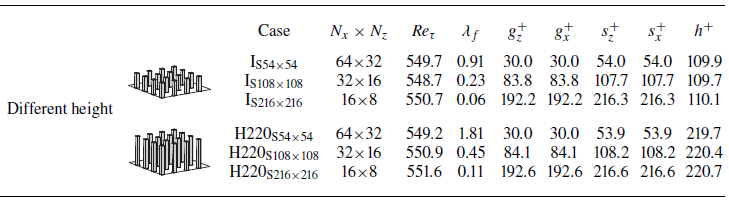


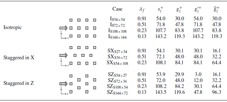


 Open access

