




No CrossRef data available.
DETECTING LACK OF IDENTIFICATION IN GMM
Published online by Cambridge University Press: 31 January 2003
Abstract
This paper proposes a test of the null of underidentification in the nonlinear-in-parameters generalized method of moments model. It can be thought of as a nonlinear analog of the usual linear instrumental variables first-stage F-test. It can be used as a diagnostic to warn a researcher when conventional asymptotic theory is unlikely to work well.I am grateful to Don Andrews, Jon Faust, John Fernald, Jim Stock, and two anonymous referees for their helpful comments on earlier drafts of this manuscript. I am also grateful to George Tauchen for providing me with the code for generating artificial asset price data. All errors are my sole responsibility.
Information
- Type
- Research Article
- Information
- Copyright
- © 2003 Cambridge University Press
1. INTRODUCTION
One of the key assumptions of the standard linear instrumental variables (IV) model is that the instruments and endogenous variables are correlated. This is the identification assumption, without which the usual IV estimator is neither consistent nor asymptotically normal. If the correlation between the instruments and the endogenous variables is nonzero, but slight, then the conventional Gaussian asymptotic theory for the IV model can nevertheless provide a very poor approximation to the actual sampling distribution of estimators and test statistics. Recognizing the identification assumption on which the IV model relies, it is quite common in the applied literature to test for instrument relevance by a first-stage F-test. The null hypothesis is one of a total lack of identification. A rejection of this hypothesis by no means implies that issues of weak instruments can be ignored (Staiger and Stock, 1997). But a failure to reject this hypothesis is a strong indication of identification difficulties. The first-stage F-test is an important and useful diagnostic in the IV model.
The generalized method of moments (GMM) model (Hansen, 1982) nests the linear IV model as a special case. Not surprisingly, analogous issues arise in this model. Researchers have found that, in many contexts, the conventional Gaussian asymptotic theory provides a poor approximation to the sampling distribution of GMM estimators and test statistics. There are many possible reasons why this could happen, but they include identification problems. However, I am aware of no test of the identification condition in the nonlinear-in-parameters GMM model in the existing literature. This paper proposes such a test. It involves an application of the general approach to testing the rank of a matrix proposed by Cragg and Donald (1997), using a Bonferroni argument to eliminate a nuisance parameter that is not consistently estimable under the null. The proposed test is, in general, asymptotically conservative.
2. THE GMM MODEL AND THE PROPOSED TEST
The GMM model specifies that {Yt}t=1T is an observed time series and θ is a p × 1 parameter vector with a true value θ0, in the interior of a compact space Θ, which has the property that

where h(.,.) is a G-dimensional function and Et(.) denotes the expectation of the argument conditional on the information set at time t. Let Zt be a k × 1 vector of instruments in this information set, with Gk ≥ p. It follows that E(φ(Yt,θ0)) = 0, where

, a Gk × 1 vector. The GMM estimator of

where S(θ) = T−1/2Σt=1Tφ(Yt,θ)′ WT(θ)T−1/2Σt=1Tφ(Yt,θ) and WT(θ) is a symmetric positive-definite weighting matrix.
Under standard assumptions, the GMM estimator is consistent and asymptotically normal and, if Gk > p, Hansen's J-test of the overidentifying restrictions is asymptotically χ2(Gk − p) distributed. But these assumptions include the requirement that the Gk × p matrix B = E [dφ(Yt,θ0)/dθ] has rank p. This is the local identification assumption and is the focus of this paper. Another standard assumption is that E(φ(Yt,θ)) has a unique zero at θ = θ0, which rules out the possibility of local but not global identification (Hsiao, 1983).
However this asymptotic theory often works poorly in practice as has been documented in Monte Carlo studies by Tauchen (1986), Kocherlakota (1990), Hansen, Heaton, and Yaron (1996), and others, and this problem can arise from weak identification. The weak identification problem in GMM may be effectively circumvented by the use of S-sets, as proposed in Stock and Wright (2000). The approach dispenses with point estimation and instead forms a confidence set for the entire parameter vector θ directly from an objective function, using a nonlinear analog of the Anderson–Rubin confidence set (Anderson and Rubin, 1949; Staiger and Stock, 1997). If T−1/2Σt=1Tφ(Yt,θ0) →d N(0,A(θ0)) for some nonsingular matrix A(θ0) and WT(θ0) →p A(θ0)−1, then S(θ0) converges to a χ2(Gk) distribution. No identification assumption is required for this to hold. The confidence set for θ is formed as the inverse of the acceptance region of this test; i.e., the confidence set of coverage 1 − α is Sθ*(α) = {θ : S(θ) ≤ Fχ2(α,Gk)} where Fχ2(a,b) is the upper 100a percentile of a χ2 distribution on b degrees of freedom. In a completely unidentified model (E(φ(Yt,θ)) = 0, uniformly in θ) or with local asymptotic underidentification (E(φ(Yt,θ)) = O(T−1/2), uniformly in θ), such a confidence set will have infinite expected volume. But under these circumstances, any valid confidence set must have infinite expected volume (Dufour, 1997). An S-set can be empty or nonconvex.
The focus of this paper is on constructing a test for detecting a lack of identification in GMM. If the test accepts the null, the researcher will know not to use conventional asymptotic theory. The S-set works regardless of whether the model is identified or not. However, a means of detecting underidentification is still useful because (a) if the model is identified, consistent point estimates of the parameters are available, (b) if the model is identified, we have confidence intervals for individual parameters that are not asymptotically conservative, unlike the confidence sets for elements of θ that can be projected from an S-set, and (c) an S-set is hard to represent when there are more than two parameters. All these advantages of using conventional asymptotics rather than the S-set are available if and only if the identification is sufficient for the conventional asymptotics to work well. The identification condition that I wish to test is that the matrix B is of rank p. I shall do this by testing the null of underidentification: that ρ(B) = r, where the operator ρ(.) denotes the rank of its argument and r < p. I define

and introduce some assumptions.
Assumption 1.

for positive-definite finite C.
Assumption 2.

is an estimator of the variance of vec[dφ(Yt,θ)/dθ] , or of 2π-times its zero-frequency spectral density matrix, such that

.
Assumption 3. T−1/2Σt=1Tφ(Yt,θ0) →d N(0,A(θ0)) for some nonsingular matrix A(θ0).
Assumption 4. WT(θ) is an estimator of 2π-times the zero-frequency spectral density matrix of φ(Yt,θ) such that WT(θ0) →p A−1(θ0).
For example, if φ(Yt,θ0) is serially uncorrelated then A(θ0) = E(φ(Yt,θ0) φ(Yt,θ0)′), and in this case one would set WT(θ) = (T−1Σt=1Tφ(Yt,θ) φ(Yt,θ)′)−1, giving the standard continuous updating estimator. Assumptions 1–4 are high-level convergence assumptions. They all apply only at the true parameter value, θ0. Let

where Ω(r) is the space of all Gk × p matrices of rank r. The proposed test statistic of the hypothesis that ρ(B) = r is L*(r) = infθ∈Sθ*(α) L(θ,r).
THEOREM 1. Under Assumptions 1–4, if B is in fact of rank r, then limT→∞ P(L*(r) ≤ Fχ2(α,(Gk − r)(p − r))) ≤ 2α.
Proof. From Theorem 1 of Cragg and Donald (1997), if ρ(B) = r then L(θ0,r) →d χ2((Gk − r)(p − r)). But limT→∞ P(θ0∈Sθ*(α)) = 1 − α and if θ0∈Sθ*(α) then L*(r) ≤ L(θ0,r), so if ρ(B) = r then limT→∞ P(L*(r) ≤ Fχ2(α,(Gk − r)(p − r))) ≤ 2α. █
The term L*(r) yields an asymptotically conservative test; the limiting probability of incorrectly rejecting the null is bounded above by 2α. This is the test statistic proposed in this paper; the test rejects if and only if L*(r) exceeds the χ2 critical value. It is a disadvantage that the proposed test is conservative, but in the context of the linear IV model there can still be severe identification difficulties even if the underidentification null is marginally rejected (Staiger and Stock, 1997), and so a conservative test may be quite useful. If ρ(B) is in fact lower than the hypothesized rank r, I conjecture (following Cragg and Donald, 1997) that the test will continue to be asymptotically conservative. If ρ(B) is higher than the hypothesized rank r, the test will reject with probability one, asymptotically. To detect identification difficulties, it is perhaps especially appropriate to test the null that ρ(B) = p − 1. In the linear IV model, L(θ,r) does not depend on θ, and there is therefore no need to eliminate θ by a Bonferroni argument as in Theorem 1; to do so would simply halve the asymptotic size of the test. Accordingly, in the linear IV model, the proposed test is no longer asymptotically conservative and instead has size equal to its nominal level, asymptotically. It reduces to the test proposed by Cragg and Donald (1993). In the case where the hypothesized rank is zero, this reduces further to the usual first-stage F-test.1
The first-stage F-test in the linear IV model however only tests the null hypothesis that all of the instruments are uncorrelated with all of the endogenous regressors; with multiple regressors this is sufficient but not necessary for underidentification (Choi and Phillips, 1992).
3. MONTE CARLO RESULTS
A leading application of the GMM method is to inference in the consumption capital asset pricing model (CAPM) with intertemporally separable constant relative risk aversion preferences. In this section, I evaluate the size and power of the proposed test in this model. The Euler equation in this model for a single asset (stocks) is as given in equation (2.1), with

where Yt = (Rt+1,Ct+1 /Ct)′, θ = (δ,γ)′, Rt is the gross stock return, Ct is consumption, δ is the discount factor, and γ is the coefficient of relative risk aversion.
In GMM estimation of this model, φ(Yt,θ) = (δRt+1(Ct+1 /Ct)−γ − 1)Zt and

Let the vector of instruments consist of an intercept, lagged returns, and lagged consumption growth, as is typical in this literature. It is hard to imagine a case in which the matrix B would have rank zero.2
This is the main reason why this paper does not simply focus on testing the hypothesis that B has zero rank, like the first-stage F-test in the linear IV model. More generally, in the linear IV model the constant is an instrument that identifies only the intercept parameter in the structural equation: this parameter is of usually of little interest, and its identifiability is overlooked by simply projecting out the constant term. No such simplification is available in the general nonlinear GMM context, so if the constant has identifying power, the matrix B must have nonzero rank.
To simulate data from the consumption CAPM, I follow the approach of Tauchen and Hussey (1991). This involves fitting a 16-state Markov chain to consumption and dividend growth calibrated so as to approximate the first-order vector autoregression (VAR):

where Dt is the dividend at date t and (uct,udt)′ is independent and identically distributed (i.i.d.) N(0,Λ).
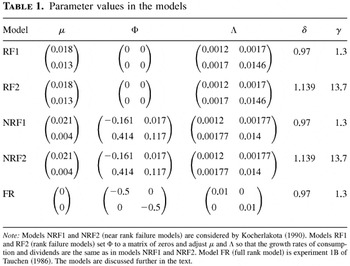
The Monte Carlo simulation in this section is based on the Euler equation in this consumption CAPM with instruments Zt = (1,Rt,Ct /Ct−1)′. I consider three sample sizes: T = 100, 500, and 1,000. The sample size of 100 is most commonly used in Monte Carlo simulations, as it is approximately equal to the available sample size for U.S. annual data. The larger sample sizes are also considered so as to include models with less severe identification problems. I consider five combinations of the parameters μ, Φ, Λ, δ, and γ, as listed in Table 1.
Parameter values in the models

The first two models set Φ equal to a matrix of zeros so as to wipe out all serial dependence in the growth rates of consumption and dividends. The true rank of B is 1 in these models; they are not fully identified, and so the rejection rate of the proposed test, used to test the hypothesis that ρ(B) = 1, represents the size of the test.3
The Euler equation can be written as vt = Et [δ(1 + vt+1)(Dt+1 /Dt)(Ct+1 /Ct)−γ] , where vt is the stock price-dividend ratio, and so if dividend growth and consumption growth are i.i.d., independent of anything in the information set at date t, then vt is constant, Rt+1 ∝ Dt+1 /Dt, and so ρ(B) = 1.
Kocherlakota (1990) chooses values of μ, Φ, and Λ by fitting a bivariate VAR(1) to historical U.S. annual real dividend growth and real consumption growth data. Models NRF1 and NRF2 use his values of these parameters. These models set δ = 0.97, γ = 1.3 and δ = 1.139, γ = 13.7. The true rank of B is 2 in these models; the models are identified, and so the rejection rate of the proposed test represents the power of the test. However, B is close to being rank deficient, and so weak identification problems may arise. Hansen et al. (1996) and Stock and Wright (2000) show that the conventional Gaussian asymptotic theory works poorly in small samples in these models. It is of interest to see how the power of the proposed test is related to the quality of the conventional asymptotic theory.
Last, model FR uses parameters for which Tauchen (1986) finds that the conventional asymptotic theory works well, even in small samples. The true rank of B is 2 in this model; the rejection rate of the proposed test represents its power.
I calculate the test statistic L*(1) as the minimum of L(θ,1) subject to the constraint S(θ) ≤ Fχ2(α,k), using Matlab optimization routines, starting from a grid of different values of θ.
4The weighting matrix is WT(θ) = (T−1Σt=1Tφ(Yt,θ)φ(Yt,θ)′)−1. Because the returns are not overlapping it is an implication of the model that φ(Yt,θ0) is serially uncorrelated.

. Any k × 2 matrix P of rank 1 can be written either as [π1 λπ1] or as [0 π2] where π1 and π2 are k × 1 vectors and λ is a scalar, so L(θ,1) can be computed by minimizing this quadratic form over all such matrices P.
5Matlab code for the computations in these Monte Carlo simulations is available from the author on request. In principle, the test statistic can be calculated in this way for any dimension of θ, but the computational cost will be considerable for high-dimensional problems.
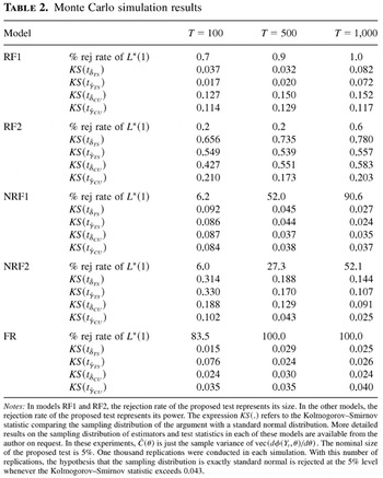
The simulated rejection rates of L*(1) for all of these models are reported in Table 2. In this table, I also report the Kolmogorov–Smirnov statistic comparing the sampling distribution of the t-statistics to the standard normal distribution, for each experiment, as a summary statistic of how well the conventional asymptotic theory works. In the underidentified models (RF1 and RF2), the conventional asymptotic theory works poorly. The problem is worse in model RF2 than in model RF1. Indeed in model RF1, the two-step t-statistics are quite close to being standard normal in samples of size 100 and 500 but then become less normal as the sample size increases, in a clear sign of a lack of identification. In models RF1 and RF2, the actual size of the proposed test is consistently well below the nominal 5% level (not surprisingly, as the test is asymptotically conservative). In model NRF1, the predictions of conventional asymptotic theory work better as the sample size increases. The proposed test has very little power in the sample of size 100, but its power increases with the sample size. In this model, with a sample size of 1,000, conventional asymptotic theory works well, and the proposed test has 90.6% power. In model NRF2, the predictions of conventional asymptotic theory work less well. Conventional asymptotic theory works poorly in a sample size of 100, but again the problems get less severe as the sample size increases. The proposed test has very little power in the sample of size 100. Its power increases with the sample size but (appropriately) does so more slowly than in model NRF1. In model FR, I find, like Tauchen (1986), that the conventional asymptotic theory works well in all sample sizes. Correspondingly, the proposed test has a very high rejection rate in all sample sizes.
Monte Carlo simulation results

In summary, the proposed test is conservative under the null whereas, in the simulations where the identification condition is satisfied, its power is strongly associated with the quality of the conventional asymptotic theory. The relationship is not a perfect one, any more than it is with the first-stage F-test in the linear IV model (Staiger and Stock, 1997).
References
REFERENCES
Anderson, T.W. &
H. Rubin
(1949)
Estimation of the parameters of a single equation in a complete
system of stochastic equations.
Annals of Mathematical Statistics
20,
46–63.CrossRefGoogle Scholar
Choi, I. &
P.C.B. Phillips
(1992)
Asymptotic and finite sample distribution theory for IV estimators
and tests in partially identified structural equations.
Journal of Econometrics
51,
113–150.CrossRefGoogle Scholar
Cragg, J.G. &
S.G. Donald
(1993)
Testing identifiability and specification in instrumental variable
models.
Econometric Theory
9,
222–240.CrossRefGoogle Scholar
Cragg, J.G. &
S.G. Donald
(1997)
Inferring the rank of a matrix.
Journal of Econometrics
76,
223–250.CrossRefGoogle Scholar
Dufour, J.M.
(1997)
Some impossibility theorems in econometrics with applications to
structural and dynamic models.
Econometrica
65,
1365–1387.CrossRefGoogle Scholar
Hansen, L.P.
(1982)
Large sample properties of generalized method of moments estimators.
Econometrica
50,
1029–1054.CrossRefGoogle Scholar
Hansen, L.P.,
J. Heaton, &
A. Yaron
(1996)
Finite sample properties of some alternative GMM estimators.
Journal of Business and Economic Statistics
14,
262–280.Google Scholar
Hsiao, C.
(1983) “Identification.” In
Z. Griliches &
M.D. Intriligator (eds.),
Handbook of Econometrics,
vol. 1.
Amsterdam:
North-Holland.
Kocherlakota, N.
(1990)
On tests of representative consumer asset pricing models.
Journal of Monetary Economics
26,
285–304.CrossRefGoogle Scholar
Staiger, D. &
J.H. Stock
(1997)
Instrumental variables regression with weak instruments.
Econometrica
65,
557–586.CrossRefGoogle Scholar
Stock, J.H. &
J.H. Wright
(2000)
GMM with weak identification.
Econometrica
68,
1055–1096.CrossRefGoogle Scholar
Tauchen, G.
(1986)
Statistical properties of generalized method of moments estimators
of structural parameters obtained from financial market data.
Journal of Business and Economic Statistics
4,
397–425.Google Scholar
Tauchen, G. &
R. Hussey
(1991)
Quadrature based methods for obtaining approximate solutions to
nonlinear asset pricing models.
Econometrica
59,
371–396.CrossRefGoogle Scholar
Parameter values in the models
Monte Carlo simulation results
 You have
Access
- 53
- Cited by