




No CrossRef data available.
INPUT–OUTPUT STRUCTURE AND NOMINAL RIGIDITY: THE PERSISTENCE PROBLEM REVISITED
Published online by Cambridge University Press: 10 June 2004
Abstract
This paper revisits an important issue concerning the persistent real effect of a shock to monetary policy. Although recent sentiment has shifted away from price stickiness toward wage stickiness in explaining persistence, the present paper shows that introducing an input–output structure tends to make the former an equally important monetary transmission mechanism. Under staggered wage setting, the well-known relative-wage effect is the only source of endogenous sluggishness in wage, and thus price, adjustments, regardless of whether there is an intermediate input. Under staggered price setting, relative wages are constant, but the presence of an intermediate input creates a real-wage effect that prevents nominal wages from deviating too much from a sticky intermediate-input price. Meanwhile, stickiness in the intermediate-input price translates directly into sluggishness in marginal-cost movement. This reinforces the endogenous rigidity in the nominal wages and makes firms' pricing decisions even more rigid. Thus, although it makes no difference in output dynamics under staggered wage setting, the input–output structure improves the ability of staggered price setting in generating persistence. As a consequence, the conventional wisdom on the equivalence of price and wage staggering may continue to hold for some reasonable parameter values.
Information
- Type
- Research Article
- Information
- Copyright
- © 2004 Cambridge University Press
INTRODUCTION
This paper revisits an important issue concerning the persistent real effect of monetary policy shocks. Following the lead of Taylor (1980) and Blanchard (1983, 1986), a growing body of literature focuses on models with staggered wage or staggered price setting in solving the persistence problem.1
Taylor (1999) provides a rather comprehensive survey of this literature.
This view, however, is challenged by Andersen (1998) and Huang and Liu (1998, 2002). These authors argue that, for plausible parameter values, staggered wage setting is better able to generate persistence than is staggered price setting in a dynamic general equilibrium framework.2
In their study of the Great Depression, Bordo et al. (2000) also demonstrate the ability of wage staggering in generating persistence in the response of real economic activity to monetary policy shocks.
Our model is a dynamic extension of Blanchard and Kiyotaki (1987), featuring monopolistic competition in goods and labor markets, in which imperfectly competitive firms set nominal prices for differentiated goods and imperfectly competitive households set nominal wages for differentiated labor skills. The model has two additional features. First, a composite of the differentiated goods can serve either as a final consumption good or as an intermediate input for producing the differentiated goods. In equilibrium the consumption price index facing the households is equal to the intermediate-input price facing the firms. Second, prices or wages are set in a staggered fashion. To obtain an analytical solution for a system of log-linearized equilibrium conditions, we abstract from capital accumulation. This simplification does not alter our basic conclusion.3
A model with capital accumulation and simulation results is available upon request from the authors.
To illustrate the intuition behind our results, let us consider what would happen following a positive aggregate demand shock. With nominal staggering of either type, part of the shock transmits into a higher demand for labor and a higher real income. As a consequence, the marginal disutility of working rises and the marginal utility of consumption falls. This would induce a household to raise its nominal wage whenever possible.
If it is wage-setting decisions that are staggered, then an increase in a household's nominal wage will lead to a rise in its relative wage. This creates an incentive for firms to substitute away from its labor service toward those of the other households. Such substitution tends to reduce the household's hours worked and marginal disutility of working, which would discourage it from raising its wage by too much. With synchronization in pricing decisions, the prices of all goods can be adjusted in any period. The intermediate-input price as a composite of individual goods' prices is thus a flexible part of firms' marginal production cost. Given that the firms set their prices equal to a markup over the marginal cost, rigidity in their pricing decisions arises entirely from rigidity in the nominal wage index, just as in the case without an intermediate input. This is why the presence of an intermediate input in this case does not affect firms' pricing behavior or the property of output dynamics.
If it is pricing decisions that are staggered, then increases in households' nominal wages, although not affecting their relative wages given synchronization in wage-setting decisions, will cause the real wage to rise in the face of the sticky intermediate-input price. A rise in the real wage creates an incentive for firms to substitute away from the composite labor toward the intermediate input. This would discourage the households from raising their nominal wages by too much. Thus, the intermediate-input price being a rigid part of firms' marginal cost results in endogenous nominal wage rigidity, which reinforces the stickiness in the intermediate-input price to generate sluggishness in the marginal-cost movement. This would in turn discourage the firms from raising their prices by too much. This is why the presence of an intermediate input improves the ability of staggered price setting in generating output persistence.
Our work is closely related to that of Edge (2002) who establishes the equivalence of wage and price staggering in the presence of labor specificity, which is a type of real rigidity in the sense of Ball and Romer (1990).4
The importance of factor specificity for enhancing the ability of a sticky-price model in generating persistence has also been studied by Gust (1997), who emphasizes capital specificity, and by Ascari (2001), who emphasizes labor specificity, as does Edge (2002).
For analytical convenience we have focused on a roundabout input–output structure in this paper, but the basic insights and conclusions presented here also hold for an inline production chain that is analyzed empirically by Clark (1999) and theoretically by Huang and Liu (2001a). With a chain structure of production, closed-form solutions are hard to obtain, and we have to rely on numerical simulations (not reported). In an open-economy setup, Bergin and Feenstra (2001) and Huang and Liu (2000, 2001b) found that international input–output connections, either roundabout or chain-like, may interact with price rigidity to help transmit monetary policy shocks across countries with trade links.
It is worth noting that we have considered only one type of real flexibility (rigidity) that is relevant across many industries in most modern economies. Our intent is to focus on why and how this type of real flexibility (rigidity) can interact differently with the two types of nominal staggering: This can best be done by isolating such interactions from the potential interference of other mechanisms.6
In general, there may exist nontrivial interactions between an input–output structure and other types of real flexibility (rigidity), which may also be important for understanding the empirical performance of models with nominal rigidity. For example, Bergin and Feenstra (2000) emphasize a nonlinear interaction between a roundabout input–output connection and translog preferences under staggered price setting that goes beyond their individual contributions in generating persistence. Dotsey and King (2001) incorporate a roundabout input–output relation, variable capacity utilization, and labor supply variability through changes along the extensive margin into a sticky-price model. They show that not only do the three types of real flexibility separately contribute to generating persistence, but “their effects on persistence are mutually reinforcing.”
For recent efforts toward this goal, see Bergin and Feenstra (2000), Edge (2000), Dotsey and King (2001), and Christiano et al. (2001), among others. In a companion paper, Huang et al. (2001) construct a model combining staggered wage and price setting with a roundabout input–output structure. They show, through numerical simulations, that the three effects identified in the present paper, namely, the relative-wage effect, the real-wage effect, and the effect of a sticky intermediate-input price being a direct entry of marginal cost, are all important for generating output persistence and for explaining the evolution of the cyclical behavior of the U.S. real wages over time.
In what follows, Section 2 sets up the model, Section 3 presents the analytical results, Section 4 conducts numerical simulations, and Section 5 concludes.
A MODEL WITH INTERMEDIATE INPUT AND NOMINAL RIGIDITY
Time is discrete and indexed by t=1, 2, …. There is a large number of households, each endowed with a differentiated labor skill indexed by i∈[0, 1], a large number of firms, each producing a differentiated good indexed by j∈[0, 1], and a government conducting monetary policy. At each date t, the economy experiences a realization of shocks st. The history of events up to date t is st=(s1, …, st) with probability π(st). The initial realization s1 is given.
Aggregation
In each event history st, the differentiated labor skills {L(i, st)}i∈[0,1] are aggregated into a composite skill L(st) according to
, and the differentiated goods {X(j, st)}j∈[0,1] are aggregated into a composite good X(st) according to
, where θl∈(1, ∞) and θx∈(1, ∞) denote, respectively, the elasticities of substitution between the differentiated skills and between the differentiated goods. The aggregation activity is perfectly competitive. The resulting demands for labor skill i and good j are given by

where the wage rate
for the composite skill and the wage rates {W(i, st)}i∈[0,1] for the differentiated skills have the relation
, and the price
for the composite good and the prices {P(j, st)}j∈[0,1] for the differentiated goods satisfy the relation
.
The defining feature of our model is that, while the composite skill can only serve as an input for the production of each differentiated good, the composite good can serve either as a final good consumed by households or as an intermediate production input used by firms.
Firms
The technology for producing a good j is represented by a constant-returns-to-scale production function,

where Γ(j, st) and L(j, st) denote the intermediate input and the composite labor, respectively, and ϕ∈(0, 1) is the share of the intermediate input in production.
8The Cobb-Douglas specification of the production function is fairly standard in the literature. See, among others, Basu (1995), Basu and Kimball (1997), Bergin and Feenstra (2000, 2001), Linnemann (2000), Hillberry and Hummels (2002), Ambler et al. (2002), and Yi (2003). We use this specification here for analytical convenience. The basic insights in this paper stand up to a more general specification of production technology with a nonunitary elasticity of substitution between the primary factor and the intermediate input, such as the CES specification of Dotsey and King (2001).
All firms are price- and wage-takers in the input markets and imperfect competitors in the output markets, where they set prices for their own outputs, taking the demand schedule (2) as given. At each date t, a fraction 1/Np of the firms chooses new prices after the realization of the shock st. Once a price is set, it remains effective for Np periods. The firms are divided into Np cohorts based on the timing of their pricing decisions. A firm j in the cohort that can choose a new price at date t solves the problem

where D(sτ|st) is the price of one dollar at sτ in units of dollars at st, and Q(sτ) is the unit cost of production at sτ (which is also the marginal cost, given the constant-returns-to-scale technology) given by

The solution to the problem stated in (4) is

According to (6), the optimal price is a markup over a weighted average of the marginal costs during the periods in which the price will remain in effect. The solution to the cost-minimization problem (5) yields the unit cost function
, where
is a constant determined by ϕ, and the demand functions for the intermediate input and the composite labor in producing Xd(j, sτ) are given by

Note that, even if a firm cannot choose a new price at a given date, it would still need to choose the inputs of the intermediate good and the composite labor in order to minimize its unit production cost. In other words, it has to solve the problem stated in (5) and, therefore, (7) and (8) hold for all firms at any time.
Households
Each household i has a subjective discount factor β∈(0, 1) and a utility function

where
is a CES composite of consumption good and real money balances, and L(i, st) denotes the household's hours worked. The period-utility function U is strictly increasing and the period-disutility function V is strictly decreasing, and both U and V are strictly concave and twice continuously differentiable. The budget constraint facing the household in event history st is

where B(i, st+1) is the household's holdings of a nominal bond, each unit of which costs D(st+1|st) dollars at st and pays off one dollar in period t+1 if st+1 is realized, W(i, st) is a nominal wage rate for its type of labor skill, Π(i, st) is its share of firms' profits, and T(i, st) is a lump-sum transfer it receives from the government.
All households are price-takers in the good markets and imperfect competitors in the labor markets, where they set nominal wages for their labor skills, taking the demand schedule (1) as given. At each date t, upon the realization of the shock st, a fraction 1/Nw of the households chooses new wages. These wages, once set, will remain in effect for Nw periods. The households are divided into Nw cohorts based on the timing of their wage decisions. Each household maximizes (9) subject to (10) and a borrowing constraint B(i, st+1)≥−B, for some large positive number B. The initial conditions on bond- and moneyholdings are taken as given. At date t, if a household i can set a new wage, then the optimal choice of its nominal wage is

where Vl(i, sτ) and Uc(i, sτ) denote its marginal disutility of labor and its marginal utility of consumption, respectively. According to (11), the optimal wage is a markup over a weighted average of dollarized marginal rates of substitution between leisure and consumption during the periods in which the wage will remain in effect. Regardless of whether they can adjust their wages at a given time, all households need to make decisions on consumption, money balances, and bondholdings in any period. We have used the standard first-order condition for bondholdings in deriving (11).
Monetary Policy
We are interested in the dynamic effect of monetary policy shocks on the fluctuations of real GDP. To serve this purpose, we assume that monetary policy is conducted via lump-sum transfers to households so that the sum of the transfers is equal to the change in money supply. That is, we assume that ∫10T(i, st)=Ms(st)−Ms(st−1)=[μ(st)−1]Ms(st−1). We also assume that the log of the growth rate of money supply lnμ(st) follows a stationary stochastic process given by

where 0<ρ<1, and εt is a white-noise process, with a zero mean and a finite variance σ2ε.
Equilibrium
An equilibrium for this economy consists of allocations C(i, st), M(i, st), B(i, st+1), and wage W(i, st) for household i, for all i∈[0, 1], allocations Γ(j, st), L(j, st), and price P(j, st) for firm j, for all j∈[0, 1], together with prices D(st+1|st),
, and wage
, that satisfy the following conditions: (i) taking the wages and all prices but its own as given, each firm's allocations and price solve its profit-maximization problem; (ii) taking the prices and all wages but its own as given, each household's allocations and wage solve its utility-maximization problem; (iii) markets for money, bonds, the composite labor, and the composite good clear; (iv) monetary policy is as specified.
We assume that there are complete financial markets that allow households to transfer their nominal wealth across dates and states and to insure one another against their exposure to idiosyncratic income risks that may arise from differences in the timing of their wage-setting decisions under staggered wage contracts. We suppose that, with such financial arrangements, the equilibrium consumption, and holdings of real money balances are identical across households, assuming an identically distributed initial wealth. It follows that C(i, st)=∫10C(i, st)di=Y(st) and M(i, st)=∫10M(i, st)di≡M(st), for all i and for every st, where Y(st) denotes real GDP.
9In this closed economy with no investment or government spending, real GDP is equal to aggregate consumption.

and the market-clearing condition for the composite labor ∫10L(j, st)dj=L(st) implies that

where
. Equations (13) and (14), together with the price-setting equation (6), the wage-setting equation (11), and the money-market-clearing condition M(st)=Ms(st), characterize an equilibrium.
ANALYTICAL RESULTS
Let N be an integer larger than 1, and assume that N periods of our model time correspond to one physical year. We consider two alternative cases, one with staggered wage setting, in which Nw=N and Np=1, and the other with staggered price setting, in which Nw=1 and Np=N. Thus N parameterizes the exogenous amount of staggering of either type. Our objective here is to inquire whether and how an input–output structure can interact differently with the two types of nominal staggering in generating persistence. Clearly, combining the two types of nominal rigidity with the input–output structure at the same time will not serve this purpose.
We proceed by first simplifying notations. In equilibrium, a household or a firm is identified by the time at which it can set a new wage or a new price. Thus, we can drop the indexes i and j for individual households and firms, replace the event argument st by the time subscript t, and denote by Wt and Pt the wage and the price set at time t, and so on. We derive analytical solutions to a loglinearized system of the equilibrium conditions, and we use lowercase letters to denote the log deviations of the corresponding level variables from their steady-state values. For simplicity, we impose a static money demand equation
for now, and we will relax this assumption in the next section.
The persistence implications of wage staggering and price staggering are embodied in the wage-setting equation and the price-setting equation, both of which take a common loglinear form

where bj=(N−j)/[N(N−1)], Et is a conditional expectation operator, and we have set β=1 to help exposition. Equation (15) corresponds to the wage-setting rule if z=w, and to the pricing-decision rule if z=p, with the two parameters γw and γp given by

where f(ϕ, θx)≡ϕ/[ϕ+θx(1−ϕ)], and ξc and ξl denote the steady-state relative risk aversions in consumption and in labor hours, given by −CU″/U′ and LV″/V′, respectively. It is worth noting that γw as determined by (16) is independent of ϕ while, given θx∈(0, ∞), the term f(ϕ, θx) is strictly increasing in ϕ, so that γp as determined by (17) is strictly decreasing in ϕ. This difference between γw and γp in relation to ϕ is the key to understanding our main result. We will come back to this shortly.
For now, let's note that the first two terms on the right-hand side of (15) imply that households or firms would like to keep their wages or prices in line with those set in the past and expected to be set in the future by their peers, which will remain in effect within their own contract duration. Taylor (1980) suggests that this backward- and forward-looking effect provides a promising avenue for generating price-level inertia and output persistence. Clearly, the magnitude of this effect is the same, as each bj is, regardless of whether it is wage decisions or price decisions that are staggered. In fact, arbitrary persistence would obtain, were wages or prices assumed to be exogenously sticky for an arbitrarily long period of time. Yet, as most empirical studies suggest, the length of nominal contracts on average is about one year [e.g., Taylor (1999)], which is much shorter than the duration of a typical business cycle.
The difficult problem is thus to generate a long period of endogenous nominal rigidity and real persistence from a short period of exogenous nominal stickiness. Endogenous nominal rigidity requires that households (firms) choose not to change their wages (prices) by much when they can adjust wages (prices), while endogenous real persistence is captured by output dynamics beyond the point in time when all households (firms) have had the chance to adjust their wages (prices), that is, beyond the initial N periods following a shock. We turn now to analyzing the determination of endogenous nominal rigidity and real persistence under each of the two types of nominal staggering.
Endogenous Nominal Rigidity
As revealed by the third term on the right-hand side of (15), the amount of endogenous nominal rigidity is inversely related to γz, which measures the response of wages or prices to a given change in expected aggregate demand conditions within a contract length. A smaller γz implies greater endogenous nominal rigidity for given exogenous nominal stickiness. Inspecting (16) and (17) reveals that whether wage and price staggering may have the same implication for endogenous nominal rigidity depends on whether γw and γp are equal.
Before looking into this possibility, we first provide some intuitions for why γw and γp are linked to the fundamental parameters via the functional forms in (16) and (17), especially, why γw is independent of ϕ whereas γp is strictly increasing in ϕ. The intuitions can best be illustrated by considering what would happen following a 1% shock to aggregate demand. With nominal staggering of either type, part of the shock transmits into a higher demand for labor and a higher real income. In consequence, the marginal disutility of working rises and the marginal utility of consumption falls. This would induce a household to raise its nominal wage whenever possible. This is why ξl (which determines how rapidly the marginal disutility of working rises as hours worked increase) and ξc (which determines how fast the marginal utility of consumption falls as consumption rises) enter the numerator of γw and of γp.
If it is wage-setting decisions that are staggered, then an increase in a household's nominal wage will lead to a rise in its relative wage. This creates an incentive for firms to substitute away from its labor service toward those of the other households. Such substitution tends to reduce the household's hours worked and marginal disutility of working, which would discourage it from raising its wage by too much. In consequence, the optimal increment in the household's wage is less than ξc+ξl. This is why ξl and θl (which determines how rapidly the amount the household works falls as its nominal wage rises) enter the denominator of γw.
As noted above, γw is independent of ϕ, the share of the intermediate input in production. This independence is one part of the key to establishing the equality between γw and γp under reasonable parameter values. To understand this independence of γw on ϕ, note that, with synchronization in pricing decisions, the price level, and thus the intermediate-input price as well, coincide with the price of each individual good that can be adjusted in any period. The price of the intermediate input is thus a flexible part of firms' marginal cost. Since the firms set their prices equal to a markup over the marginal cost, rigidity in their pricing decisions arise entirely from rigidity in the nominal wage index, regardless of the share of the intermediate input. In other words, the presence of the intermediate input does not affect the pricing behavior of the firms or the property of output dynamics. In fact, the optimal adjustment of each firm's price is given by γw, which is equal to the exact change in the nominal wage index, just as in the case with no intermediate input at all.
If it is pricing decisions that are staggered, then increases in households' nominal wages, while not affecting their relative wages, given synchronization in wage-setting decisions, will cause the real wage to rise in the face of the sticky intermediate-input price. A rise in the real wage creates an incentive for firms to substitute away from the composite labor toward the intermediate input. This would discourage the households from raising their nominal wages by too much. Therefore, the intermediate-input price being a rigid part of firms' marginal cost results in endogenous nominal wage rigidity. As a consequence, the optimal increase in the households' nominal wages, which in the present case coincides with the nominal wage index, is less than ξc+ξl. This is why f(ϕ, θx) and ξl enter the denominator of γp.
To understand the term f(ϕ, θx), we note that it corresponds to the elasticity of demand for the composite labor with respect to the real wage, with the real aggregate demand being the shift variable in the demand schedule for the composite labor.10
This should be in contrast with θl, which corresponds to the elasticity of demand for each individual labor skill with respect to its relative wage, with the composite labor being the shift variable in the demand schedule for the individual labor skill. With synchronization in wage-setting decisions, relative wages are equal to one and the demand for each individual labor skill coincides with the demand for the composite labor.
On the other hand, for any given ϕ∈(0, 1), the term f(ϕ, θx) is decreasing in θx. This is so because a larger θx corresponds to a greater elasticity of substitution between differentiated intermediate goods and firms would be able to rely less on substitution between the composite labor skill and the composite intermediate good while more on the substitution between the differentiated intermediate goods. As a consequence, when θx increases, firms' demand for the composite labor skill becomes less sensitive to changes in the real wage, and thus f(ϕ, θx) falls. This tension between the two dimensions of factor substitutions is present only if both labor and intermediate goods are used in production. This is why θx enters the term only if ϕ ≠ 0 and ϕ≠1.
To understand why the term (1−ϕ) appears in the numerator of γp, we observe that, with ϕ share of the intermediate input in production, a firm's marginal cost is composed of ϕ fraction of the price level and of (1−ϕ) fraction of the nominal wage index. Thus, exogenous nominal stickiness in the form of staggered price setting translates directly into the sluggishness in the movement of this former part of the marginal cost. Since the firm's optimal price is a markup over a weighted average of the marginal costs within its contract duration, we can scale down ϕ fraction of the rise in the nominal wage index to get the firm's optimal price response.
The fact that f(ϕ, θx) is increasing in ϕ and (1−ϕ) is decreasing in ϕ implies that γp is a decreasing function of ϕ. This monotone relation is the other part of the key to establishing the equality between γw and γp and thus the equivalent implications of wage and price staggering for endogenous nominal rigidity under reasonable parameter values.
Endogenous Real Persistence
We turn now to endogenous real persistence. Naturally, the amount of output persistence is negatively related to γz. The smaller γz is, the smaller and the less rapid are the responses of nominal prices to an aggregate demand shock, and thus the larger and the more persistent are the responses of real output to the shock. We illustrate here this inverse relationship between γz and output persistence by obtaining explicit solutions of the equilibrium dynamics for the case with N=2.
To proceed, we note that, when N=2, equation (15) simplifies to

Substituting into (18) the static money demand equation and the equation defining the price level,
, we obtain a second-order difference equation in pt as follows:

Assuming that the money stock mt follows a random-walk process, we obtain from (19) a closed-form solution for equilibrium output dynamics:

The autoregressive coefficient az in (20) determines how gradually the initial response of yt to a money supply shock will die out over time, that is, it determines how persistent the output response will be. The larger az is, the more persistent is the output response. The second equation in (20) shows that az is a strictly decreasing function of γz. Therefore, the amount of output persistence is greater, the smaller is γz. For any γz between 0 and 1, az is also between 0 and 1, and there exists endogenous output persistence. That is, the initial response of output dies out monotonically, but not completely even at the end of the initial contract duration. If γz=0, then az=1, so that output dynamics follow a random-walk process. If γz=1, then az=0, and there is no endogenous output persistence. In the case that γz>1, we have az<0, and there is oscillation rather than persistence in output dynamics. The one-to-one inverse correspondence between γz and az indicates that, whether wage and price staggering are equally capable of generating real persistence depends on whether γw and γp are equal.11
Theoretical Possibility
In light of the above analysis, the ability of staggered wage setting relative to staggered price setting in propagating a monetary policy shock is tied to the magnitude of γw relative to γp. We summarize here the theoretical implications of our analysis on the relative ability of the two types of nominal staggering in generating endogenous nominal rigidity and real persistence under general parameter values. This summary also helps connect our results to the literature.
According to (16) and (17), the intermediate-input share ϕ enters into γw and γp in different ways, implying that the use of the intermediate input in production interacts differently with the two types of nominal staggering: while it makes no difference in equilibrium dynamics under staggered wage setting (for γw is independent of ϕ), it improves the ability of staggered price setting in generating endogenous nominal rigidity and real persistence (for γp is a decreasing function of ϕ).
This observation suggests that the ability of price staggering relative to wage staggering in generating persistence depends critically on whether the use of intermediate input is taken into account. In the extreme case that ϕ is set to zero, γp is larger than γw, and it is less likely to generate persistence under staggered price setting than under staggered wage setting [e.g., Andersen (1998) and Huang and Liu (1998, 2002)]. With a positive value of ϕ, γp can be equal to or less than γw, and thus persistence can be the same or even more under staggered price setting than under staggered wage setting. In particular, for any values of the other parameters in the model, there exist values of ϕ between 0 and 1 such that γp=γw. In the extreme case that ϕ is set arbitrarily close to one, γp is arbitrarily close to zero, and arbitrary persistence obtains under staggered price setting, while the implication on persistence of staggered wage setting remains the same, just as in the case when ϕ is set to zero.
The above discussion indicates that, as long as the value of ϕ is larger than zero, it is theoretically possible that staggered price setting is as able as staggered wage setting in generating persistence. The next question is whether the equivalence of price and wage staggering can arise under empirically reasonable parameter values.
Empirical Plausibility
We now show that, once the use of intermediate input is taken into account, the equivalence of price and wage staggering in generating endogenous nominal rigidity and real persistence is not only theoretically possible, but also empirically plausible. For concreteness, we provide examples in which γp and γw can be equal under some reasonable parameter values, so that the two types of nominal staggering can be equally important transmission mechanisms of monetary shocks.
To proceed, we first note that, by virtue of (16) and (17), γp and γw are equal if and only if

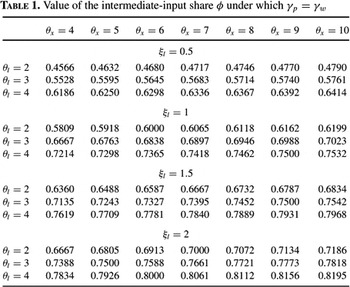
We next discuss whether this equality can hold with empirically reasonable parameter values. According to the estimates by Griffin (1992, 1996), a plausible range of θl, the elasticity of substitution between differentiated labor skills, is from 2 to 4. A reasonable range of θx, the elasticity of substitution of differentiated goods, is from 4 to 10, in light of the empirical studies by Domowitz et al. (1986), Shapiro (1987), Basu (1996), Basu and Kimball (1997), Basu and Fernald (1994, 1995, 1997), and Linnemann (1999). To pinpoint a range for the relative-risk-aversion parameter ξl, one usually appeals to the estimates of the intertemporal hours elasticity of substitution based on the intensive margin. Earlier studies along this avenue mostly suggest that this elasticity is smaller than 1 [see, e.g., the survey by Pencavel (1986)]. More recent work demonstrates that these earlier estimates can be subject to large downward biases [e.g., Rupert, Rogerson, and Wright (2000)]. In particular, Mulligan (1999) finds that the elasticity is instead in the range from 1 to 2. Recent studies also show that the employment elasticity based on the extensive margin can be much greater than 1 [e.g., Kimmel and Kniesner (1998)]. We consider the value of ξl from 0.5 to 2, corresponding to the intertemporal labor elasticity of substitution between 2 and 0.5.
Table 1 displays the intermediate-input share ϕ (between 0 and 1) that solves (21) under the above values of θl, θx, and ξl. Some of these values of ϕ are consistent with the empirical evidence. For example, the estimates by Jorgenson et al. (1987) suggest that the value of ϕ is at least 0.5 for U.S. manufacturing industries over the period 1947–1979. Nevo (2001) finds that the share of raw materials in the U.S. food industry (SIC 20) is 0.634, based on the Annual Survey of Manufacturers over the period 1988–1992. The recent empirical study by Hanes (1999) reveals that the input–output connections in the actual economy have become more sophisticated in the recent years than in the further past. This suggests an increasing intermediate-input share over time. Basu (1995) argues that the value of ϕ can lie between 0.8 and 0.9 if fixed costs are taken into account [see also Bergin and Feenstra (2000)]; yet, the implied markup drawn from Domowitz et al. (1988) is often viewed as somewhat large.

In light of the above discussion, we consider 0.5–0.7 as a reasonable range for ϕ. We then note that many values in Table 1 lie in this range or in its close vicinity. Therefore, for some empirically plausible values of the fundamental parameters, price and wage staggering can be two equivalent mechanisms in generating endogenous nominal rigidity and real persistence.12
With a separable utility (9) in consumption and leisure, the balanced-growth-path property requires that ξc=1. Then, for all the values of θl, θx, ξl, and ϕ displayed in Table 1, the corresponding values of γw and γp are not only equal, but less than 1, and there is an equal amount of endogenous persistence under staggered price setting and under staggered wage setting.
NUMERICAL SIMULATIONS
To check the robustness of our analytical results, we conduct numerical simulations with an interest-sensitive money demand equation derived from households' optimizing behavior. We set N=4 so that one period in our model corresponds to one quarter of a physical year. We choose the AR(1) coefficient ρ in the money growth process (12) equal to 0.57, in light of a money growth regression based on quarterly U.S. M1 data and as is standard in the literature [e.g., Chari et al. (2000)]. We set β=0.99, ξc=1, ξl=1, θl=2, and θx=10, which are all standard values used in the literature.
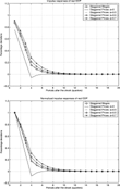
We generate the impulse response of real GDP to a one percentage shock in the money growth innovation ε0 under wage and price staggering for various values of the intermediate-input share ϕ. We find that the impulse response function under staggered wage setting stays the same regardless of the value of ϕ, while the impulse response function under staggered price setting becomes flatter as the value of ϕ grows larger. These impulse response functions are plotted in Figure 1, with the upper panel displaying the actual impulse responses and the lower panel displaying the normalized impulse responses.

The figure confirms our analytical result that a greater intermediate-input share helps generate more persistence under staggered price setting, while it makes no difference in output dynamics under staggered wage setting. In the extreme case that ϕ is set to zero, there is more persistence under wage staggering than under price staggering. As ϕ increases from zero, persistence under price staggering increases whereas persistence under wage staggering remains the same. As ϕ increases from 0.5 to 0.7, the former catches up with and eventually exceeds the latter. Thus, once the empirically relevant input–output structure is taken into account, staggered price setting may be as capable as staggered wage setting in generating persistence for some reasonable parameter values.
CONCLUDING REMARKS
We have shown that the presence of an input-output production structure helps generate more persistent response of real output to an aggregate demand shock under staggered price setting, but it makes no difference in output dynamics under staggered wage setting. With price staggering, the input–output structure creates a real-wage effect that prevents nominal wages from deviating too much from a sticky intermediate-input price. This endogenous rigidity in the nominal wages reinforces the stickiness in the intermediate-input price to increase rigidity in firms' pricing decisions and thus output persistence. With wage staggering, rigidity in firms' pricing decisions arises entirely from nominal wage rigidity produced by a relative-wage effect, just as in the case without an input–output structure. In other words, the presence of an input–output structure does not affect firms' pricing behavior or the property of output dynamics under staggered wage setting. As a consequence, the conventional wisdom on the equivalence of wage and price staggering in generating persistence may continue to hold with optimizing individuals and some plausible values of fundamental parameters, once an empirically relevant input–output structure is taken into account.
The results obtained here suggest that modeling the input–output connections in actual economies may be important for better understanding some standing economic issues. Recent empirical studies reveal that the sophistication of the input–output relations has increased over the years, both within the United States [e.g., Hanes (1999)] and in the global economy [e.g., Feenstra (1998), Hummels et al. (1998, 2001)]. Future research that captures this real-world feature should be both important and promising. The present paper only represents a small step toward this direction.
We are grateful to two anonymous referees and an Associate Editor of this journal for their very useful comments and suggestions that have led to substantial improvements in the paper. We also thank V.V. Chari, Todd Clark, Joe Haslag, Sharon Kozicki, and Stacey Schreft for helpful conversations. The views expressed herein are those of the authors and do not necessarily reflect the views of the Federal Reserve Bank of Kansas City or the Federal Reserve System.
References
Ambler S.,
E. Cardia &
C. Zimmermann
2002
International transmission of the business cycle in a multi-sector model.
European Economic Review
46,
273–
300.Google Scholar
Andersen T.M.
1998
Persistency in sticky price models.
European Economic Review
42,
593–
603.Google Scholar
Ascari G.
2000
Optimizing agents, staggered wages and persistence in the real effects of money shocks.
Economic Journal
110,
664–
686.Google Scholar
Ascari G.
2001
Price/Wage Staggering and Persistence: A Unifying Framework.
Mimeo, University of Pavia.
Ball L. &
D. Romer
1990
Real rigidity and the non-neutrality of money.
Review of Economic Studies
57,
183–
203.Google Scholar
Basu S.
1995
Intermediate goods and business cycles: Implications for productivity and welfare.
American Economic Review
85,
512–
531.Google Scholar
Basu S.
1996
Procyclical productivity: Increasing returns or cyclical utilization?
Quarterly Journal of Economics
111,
719–
751.Google Scholar
Basu S. &
J.G. Fernald
1994
Constant Returns and Small Markups in U.S. Manufacturing.
International Finance discussion paper 483, Board of Governors of the Federal Reserve System.
Basu S. &
J.G. Fernald
1995
Are apparent productive spillovers a figment of specification error?
Journal of Monetary Economics
36,
165–
188.Google Scholar
Basu S. &
J.G. Fernald
1997
Returns to scale in U.S. production: Estimates and implications.
Journal of Political Economy
105,
249–
283.Google Scholar
Basu S. &
M.S. Kimball
1997
Cyclical Productivity with Unobserved Input Variation.
NBER working paper 5915.
Bergin P. &
R.C. Feenstra
2000
Staggered price setting, translog preferences, and endogenous persistence.
Journal of Monetary Economics
45,
657–
680.Google Scholar
Bergin P. &
R.C. Feenstra
2001
Pricing-to-market, staggered contracts, and real exchange rate persistence.
Journal of International Economics
54,
333–
359.Google Scholar
Blanchard O.J.
1983
Price asynchronization and price level inertia.
In R. Dornbusch &
M.H. Simonsen (eds.),
Inflation, Debt, and Indexation
, pp. 3–
24.
Cambridge, MA:
MIT Press.
Blanchard O.
1986
The wage price spiral.
Quarterly Journal of Economics
101,
543–
565.Google Scholar
Blanchard O.J. &
N. Kiyotaki
1987
Monopolistic competition and the effects of aggregate demand.
American Economic Review
77,
647–
666.Google Scholar
Bordo M.D.,
C.J. Erceg &
C.L. Evans
2000
Money, sticky wages, and the Great Depression.
American Economic Review
90,
1447–
1463.Google Scholar
Chari V.V.,
P.J. Kehoe &
E.R. McGrattan
2000
Sticky price models of the business cycle: Can the contract multiplier solve the persistence problem?
Econometrica
68,
1151–
1180.Google Scholar
Christiano L.J.,
M. Eichenbaum &
C.L. Evans
2001
Nominal Rigidity and the Dynamic Effect of a Shock to Monetary Policy.
NBER working paper 8402.
Clark T.E.
1999
The responses of prices at different stages of production to monetary policy shocks.
Review of Economics and Statistics
81,
420–
433.Google Scholar
Domowitz I.R.,
G. Hubbard &
B.C. Petersen
1986
Business cycles and the relationship between concentration and price-cost margins.
Rand Journal of Economics
17,
1–
17.Google Scholar
Domowitz I.R.,
G. Hubbard &
B.C. Petersen
1988
Market structure and cyclical fluctuations in U.S. manufacturing.
Review of Economics and Statistics
70,
55–
66.Google Scholar
Dotsey M. &
R.G. King
2001
Pricing, Production and Persistence.
NBER working paper 8407.
Edge R.M.
2000
Time-to-Build, Time-to-Plan, Habit-Persistence, and the Liquidity Effect.
International Finance discussion paper 673, Board of Governors of the Federal Reserve System.
Edge R.M.
2002
The equivalence of wage and price staggering in monetary business cycle models.
Review of Economic Dynamics
5,
559–
585.Google Scholar
Feenstra R.C.
1998
Integration of trade and disintegration of production in the global economy.
Journal of Economic Perspectives
12,
31–
50.Google Scholar
Griffin P.
1992
The impact of affirmative action on labor demand: A test of some implications of the Le Chatelier principle.
Review of Economics and Statistics
74,
251–
260.Google Scholar
Griffin P.
1996
Input demand elasticities for heterogeneous labor: Firm-level estimates and an investigation into the effects of aggregation.
Southern Economic Journal
62,
889–
901.Google Scholar
Gust C.J.
1997
Staggered Price Contracts and Factor Immobilities: The Persistence Problem Revisited.
Manuscript, Northwestern University.
Hanes C.
1999
Degrees of processing and changes in the cyclical behavior of prices in the United States, 1869–1990.
Journal of Money, Credit, and Banking
31,
35–
53.Google Scholar
Hillberry R. &
D. Hummels
2002
Explaining Home Bias in Consumption: The Role of Intermediate Input Trade.
NBER working paper 9020.
Huang K.X.D. &
Z. Liu
1998
Staggered Contracts and Business Cycle Persistence.
Institute for Empirical Macroeconomics discussion paper 127, Federal Reserve Bank of Minneapolis.
Huang K.X.D. &
Z. Liu
2000
Vertical International Trade as a Monetary Transmission Mechanism in an Open Economy.
Cahiers de Recherche CREFE/CREFE working paper 107,
CREE, Universitat du Quebec at Montreal.
Huang K.X.D. &
Z. Liu
2001a
Production chains and general equilibrium aggregate dynamics.
Journal of Monetary Economics
48,
437–
462.Google Scholar
Huang K.X.D. &
Z. Liu
2001b
An Input–Output Channel of International Monetary Policy Transmissions.
Mimeo, Federal Reserve Bank of Kansas City.
Huang K.X.D. &
Z. Liu
2002
Staggered price setting, staggered wage setting, and business cycle persistence.
Journal of Monetary Economics
49,
405–
433.Google Scholar
Huang K.X.D.,
Z. Liu &
L. Phaneuf
2001
On the Transmission of Monetary Policy Shocks.
Mimeo, Federal Reserve Bank of Kansas City.
Hummels D.,
D. Rapoport &
K. Yi
1998
Vertical specialization and the changing nature of world trade.
Federal Reserve Bank of New York Economic Policy Review
4
(2),
79–
99.Google Scholar
Hummels D.,
J. Ishii &
K. Yi
2001
The nature and growth in vertical specialization in world trade.
Journal of International Economics
54,
75–
96.Google Scholar
Jorgenson D.W.,
F.M. Gollop &
B.M. Fraumeni
1987
Productivity and U.S Economic Growth..
Cambridge, MA:
Harvard University Press.
Kimmel J. &
T.J. Kniesner
1998
New evidence on labor supply: Employment versus hours elasticities by sex and marital status.
Journal of Monetary Economics
42,
289–
302.Google Scholar
Linnemann L.
1999
Sectoral and aggregate estimates of the cyclical behavior of markups: Evidence from Germany, Weltwirtschaftliches Archiv.
Review of World Economics
135,
480–
500.Google Scholar
Linnemann L.
2000
Intermediate Goods, Real Rigidity, and Output Persistence.
Working paper, University of Cologne.
Mulligan C.B.
1999
Substitution over time: Another look at life cycle labor supply.
In B.S. Bernanke &
J.J. Rotemberg (eds.),
NBER Macroeconomics Annual.
Cambridge, MA:
MIT Press.
Nevo A.
2001
Measuring market power in the ready-to-eat cereal industry.
Econometrica
69,
307–
342.Google Scholar
Pencavel J.
1986
The labor supply of men: A survey.
In O.C. Ashenfelter &
L. Richard (eds.),
Handbook of Labor Economics,
vol. 1, pp. 3 –102.
Amsterdam:
North-Holland.
Rupert P.,
R. Rogerson &
R. Wright
2000
Homework in Labor Economics: Household Production and Intertemporal Substitution.
Journal of Monetary Economics
46,
557–
579.Google Scholar
Shapiro M.D.
1987
Measuring Market Power in U.S. Industry.
NBER working paper 2212.
Taylor J.B.
1980
Aggregate dynamics and staggered contracts.
Journal of Political Economy
88,
1–
23.Google Scholar
Taylor J.B.
1999
Staggered Price and Wage Setting in Macroeconomics.
In J.B. Taylor &
M. Woodford (eds.),
Handbook of Macroeconomics,
vol. 1, pp. 1009–1050.
Amsterdam:
North-Holland.
Yi K.M.
2003
Can vertical specialization explain the growth of world trade?
Journal of Political Economy
111,
52–
102.Google Scholar
Value of the intermediate-input share ϕ under which γp=γw
 You have
Access
- 26
- Cited by