

Introduction
Ethiopia is believed to have the largest livestock population in Africa. Results of the latest livestock population census showed about 53.4 million heads of cattle (CSA, 2010/11), without including cattle populations of three zones of Afar and six zones of Somali Regions. The majority (99.26 percent) of the cattle population are local breeds, which are found in rural areas under subsistence mode of farming. Cross-bred and pure exotic cattle accounted for about 0.64 and 0.1 percent, respectively (CSA, 2010/11).
Apart from the large cattle population widely distributed throughout the country, the multiple production and service functions of cattle are crucial in the livelihoods of farmers and pastoralists. They serve as sources of milk, meat, hide, draft power and manure as well as contribute to nutrient recycling at the farm level (Getachew and Gashaw, Reference Getachew and Gashaw2001). Moreover, at the level of the national economy, the livestock sector contributes 26 percent of the agricultural gross domestic product (GDP) and 12 percent to the national GDP (CSA, 2008/09).
Based on the available information as summarized in Domestic Animal Genetic Resources Information System (DAGRIS) database (DAGRIS, 2011) there are 33 recognized indigenous cattle breeds in Ethiopia. Lately some more breed types have been identified and reported, such as the Wegera, Dembia and Mahibere-silassie breeds in the north-west (Wuletaw, Reference Wuletaw2004), Abergalle and Irob cattle breeds in the north (Zerabruk and Vangen, Reference Zerabruk and Vangen2005), Gojjam Highland zebu and Fogera breeds in the central highlands (Getachew, Reference Getachew2006) and Wollo Highland, Raya Sanga and Afar Sanga in the north-east (Tadesse, Reference Tadesse2005). However, only a small number of recognized cattle breed types have a fair description of their physical appearance, indications of their level of production, reproduction and genetic attributes (Ayalew et al., Reference Ayalew, Rege, Getahen, Tibbo and Mamo2004). Owing to lack of specific information, cattle of the present study area are generally referred to in the existing literature as Goffa zebu or Goffa Dwarf (Epstein, Reference Epstein1971; Payne and Hodges, Reference Payne and Hodges1997; Rege and Tawah, Reference Rege and Tawah1999). This does not reflect the current phenotypic diversity of the cattle populations in the Gamo Goffa zone of south-western Ethiopia.
Phenotypic as well as genetic characterization of indigenous livestock genetic resources provides the basis for any livestock development intervention. Clearly, sustainable utilization of local breeds is the best means of conserving these genetic resources. The first essential step towards sustainable utilization of these resources is to identify the major breed types, establish their population size as well as their geographical distribution and describe their typical qualitative and quantitative phenotypic traits (Negussie and Ayalew, Reference Negussie and Ayalew2002). On that basis, the present study was conducted to survey local cattle types in the Gamo Goffa zone to test the general hypothesis that the local cattle populations of this zone are phenotypically homogenous.
Materials and methods
Description of study area
This study was conducted in Gamo Goffa zone of south-western Ethiopia. Gamo Goffa zone is one of 13 zones of the Southern Nations, Nationalities and Peoples Regional State (SNNPRS) and consists of 15 rural districts and two town administrations. It is situated near the centre of the region around 5°57″–6°71″N latitude and 36°37″–37°98″E longitude. Its general elevation ranges from 600 to 3500 m asl; it receives 600–1600 mm rainfall per annum and annual temperature ranges from 10°C to 34°C (Gamo Goffa zone ARDD, 2010). Agro-ecological features of each study sites are presented in Table 1 below.
Description of the study sites.

The topography of the zone is characterized by undulating landscapes that favour the existence of different climatic zones. The total human population of the zone was reported as about 1.6 million (CSA, 2008/09) with a population density of 80 inhabitants per km2.
The farming practices are mainly mixed crop–livestock systems, with crops being more dominant in the higher altitude areas and livestock being more significant in lowland areas. According to CSA (2010/11), the estimated livestock population and beehives of Gamo Goffa zone were 1 438 752 cattle, 800 704 sheep, 336 941 goats, 128 054 equines, 1 050 744 chickens and 60 996 beehives.
Study population
Indigenous cattle populations in the Gamo Goffa zone and households keeping cattle constitute the study population.
Sample size and sampling method
To define the sampling frame, available background information on the existence of phenotypically unique cattle populations in Gamo Goffa zone was surveyed through single rapid exploratory field visits to the study area coupled with focus group discussions and review of available secondary information. Based on that information, 15 rural districts of the study zone were categorized into three groups matching three presumably distinct cattle population types. These were cattle populations of highlands, mid altitude areas and the lowland area. Three sample districts (Bonke, Chencha and Boreda) from highlands and two districts (Arba-Minch-Zuria and Mirab-Abaya) from lowlands were selected for actual data collection. Cattle populations of the mid-altitude areas did not show distinct features that make them different from those of the highland and lowland areas, and instead appeared to have intermediate features of other two types. Therefore, samples were not taken from mid-altitude districts. Five study districts were selected purposively taking into account the dominant agro-ecological zone of the districts, local knowledge on cattle population types and size of the cattle population.
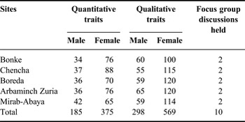
Linear body measurements were taken from 560 mature animals that were randomly selected from herds of representative households. Data on qualitative body form and shape were taken from a total of 867 animals (Table 2). The target number of sample cattle for a study site was 50–100 adult cows and about 30 bulls (FAO, 2012). Local cattle populations from similar agro-ecology were considered as similar in their phenotypic features, which were later verified by outcomes of focus group discussions. In order to base the phenotypic characterization on the mature body size of sample populations, morphometric measurements were taken from animals of at least 3 years of known age, or those with all their milk teeth erupted (i.e. full mouth). Elders, village leaders and individuals with extensive knowledge on unique history of existing cattle populations were selected in consultation with local agricultural extension workers for focus group discussions.
Sample sizes by study site.

Data collection methods
Focus group discussion
Preliminary field visits were made after gathering secondary data from local livestock extension staff about the type and distribution of indigenous cattle types in the study area. Then key informant focus group discussions were held with representatives of farmer groups, extension staff and the district administration officers. A total of ten focus group discussions were held – two per site, each having 8–12 farmers plus a representative of the extension staff. The researcher facilitated the discussion at all sites. The main points for discussion included indigenous knowledge about history of origin and introduction of existing cattle types, distinctive features of the cattle types as well as their desirable and undesirable characteristics, utility and status of the existing cattle populations and other information related to indigenous cattle.
Observations and linear body measurements
Majority of both quantitative and qualitative variables recorded in this study were adapted from the standard cattle breed descriptor list of FAO (2012). In addition, FAO (1984, 1986) cattle breed descriptor lists that were extensively reviewed and applied in Ethiopia (Wuletaw, Reference Wuletaw2004; Tadesse, Reference Tadesse2005; Taye, Reference Taye2005) were considered and a final list of variables was developed.
Depending on FAO (2012) guideline and identified cattle population type, their distribution in the study area, 185 mature adult males (both intact and castrated) and 375 heifers and cows were randomly selected for morphometric measurements. Therefore, a total of 569 female and 298 male cattle were sampled for recording their qualitative traits. A total of 16 qualitative traits were observed: coat colour pattern, coat colour type, facial profile, muzzle colour, presence of horn, horn shape, horn orientation, ear shape, ear orientation, rump profile, facial profile, hump shape, hump location, naval flap size, udder size and teat size. Similarly, 15 quantitative traits were measured in different age categories of adult animals. Quantitative traits considered include: body length, height at wither, heart girth, neck length, ear length, tail length, horn length, pelvic width, hump length, hock circumference, canon bone circumference, dewlap width, preputial sheath width, muzzle circumference and navel flap length. Measurements were taken from each trait using textile tape measurement in centimetre unit. Heart girth was measured in the early morning before the animals were taken to grazing and watering areas.
Data management and statistical analysis
All data were entered, cleaned and managed using MS Excel© worksheet. Box plots, scatter plots and tests of normality were done to check normality of quantitative variables prior to taking data to analysis.
Information compiled from focus group discussions was summarized and synthesized to describe the origin, distribution, major characteristics and status of the respective cattle populations.
Qualitative data collected were subjected to the frequency procedure of SAS (2002) version 9.0. Chi-square tests were employed to test for the difference between the factors of interest between sites. The pair-wise comparisons for each of the categorical variables across sites based on P-value were derived from Bonferroni's correction (Petrie and Watson, Reference Petrie and Watson1999).
The importance of each quantitative variable in explaining phenotypic differences between sample cattle populations of the five sites was examined using the generalized linear model (GLM) of SAS (2002). The generated site least squares means of each of the variable were then compared using Tukey's test of multiple comparison (Klockars, Hancock and McAweeney, Reference Klockars, Hancock and McAweeney1995). Considering known physiological differences among female and male animals in the measured quantitative variables, data were analysed separately for the two sex groups. The following model was used for analysing quantitative phenotypic variation between the female sample populations by considering site and parity as fixed main effects:
 $$Y_{ijk}=\mu+S_i+P_j+e_{ijk}\comma \;$$
where Y ijk is the observed value of the linear body measurements, μ is the overall mean, S i is the fixed effect of site i (i = 1…5), P j is the fixed effect of parity j (j = 1…3), where parity was categorized as 0–2 = 1, 3–4 = 2 and >4 = 3, and e ijk is the residual error.
Similarly, taking site and age class as fixed main effects, the following model was used to analyse quantitative data from males:
 $$Y_{ijk}=\mu+S_i+A_j+e_{ijk}\comma \;$$
where Y ijk is the observed value of the linear body measurements, S i is the fixed effect of site i (i = 1…5), A j is the fixed effect of age class j (j = 1…3), where age in years was categorized as 3–5 = 1, >5–7 = 2 and >7 years = 3, and e ijk is the residual error.
All interaction effects for both models were not statistically significant and so dropped from the final model.
Discriminant analysis was used on quantitative variables to classify the sampled populations into homogenous groups on the basis of the measured variables (Afifi and Clark, Reference Afifi and Clark1996; SAS, 2002). For canonical discriminant analysis (CANDISC), Mahalanobis' distance was used to check distance between measured populations. The stepwise discriminant (STEPDISC) analysis was employed to identify variables for their relative importance in discriminating between identified groups (SAS, 2002). Non-parametric discriminant analysis was performed to check importance of categorical variable in classifying the sample populations into homogenous groups.
Discriminant analysis models used to derive classification function for the female and male sample populations, respectively, are shown below:
 $$\eqalign{{\rm SF}_i &= C_i + w_i {\rm BL} + w_i {\rm CBC} + w_i {\rm TL} + w_i {\rm HW} + w_i {\rm DW} \cr &\qquad + w_i {\rm EL} + w_i {\rm HG} + w_i {\rm HL} + w_i {\rm MC} + w_i {\rm NPL} + w_i {\rm PW} \cr &\qquad + w_i {\rm HC} + w_i {\rm HP} + w_i {\rm AB\comma} \cr {\rm SM}_i &= C_i + w_i {\rm BL} + w_i {\rm CBC} + w_i {\rm TL} + w_i {\rm DW} + w_i {\rm EL} \cr &\qquad+ w_i {\rm HG} + w_i {\rm HL} + w_i {\rm HP}+ w_i {\rm MC} + w_i {\rm PSW}\cr &\qquad + w_i {\rm PW} + w_i {\rm HW} + w_i {\rm AB} + w_i {\rm HC}\comma \;}$$
where subscript ‘i’ denotes the respective group, C i is a constant for the ith group, w i is the weight of the corresponding variable in the computation of the classification score for the ith group, SF i is the resultant classification score in female population, SM i is the classification score in male population, BL is the body length, CBC is the canon bone circumference, DW is the dewlap width, EL is the ear length, HG is the heart girth, HL is the horn length, HP is the hump length, HC is the hock circumference, MC is the muzzle circumference, NL is the navel length, PW is the pelvic width, HW is the wither height, PSW is the preputial sheath width, AB is the neck length and TL is the tail length.
Results and discussion
Quantitative variation
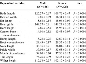
All the quantitative dependent variables were significantly (P < 0.05) affected by sex of the animal (Table 3), confirming the widely held notion that male and female populations have markedly different body form as measured in the quantitative variables. As a result, analyses of variance (ANOVAs) on quantitative variables were performed separately for the two sexes.
Least square means ± SE of quantitative body measurements (cm) for all sites by sex.

ANOVA of quantitative traits in the male sample population
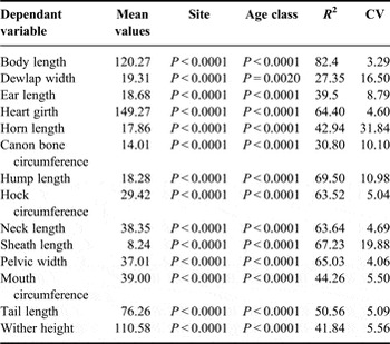
The overall phenotypic variation in all qualitative traits was highly significantly (P < 0.0001) affected by site and age class of the animals (Table 4). Since no interaction was found statistically significant, only main effects were considered. The highest (82.4 percent) rate of determination (R 2) values was calculated for body length and the smallest value for dewlap width (27.35 percent). In male sample populations, coefficients of variability ranged from 3.29 for body length to 31.84 percent for horn length.
Level of significance of main effects for quantitative variables and their associated R 2 values for the male sample population.

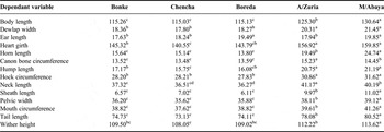
Pair-wise comparisons of the least squares means of variables between sites (Table 5) revealed that male sample populations from Mirab-Abaya and Arbaminch-Zuria districts had the largest measurement values for all variables than from Bonke, Chencha and Boreda districts. This shows that cattle populations sampled from lowland sites were larger in their linear measurements than highland ones. As presented in Table 5, samples from Chencha followed by sample populations from Boreda and Bonke had significantly lower least squares means for most of quantitative variables.
Least squares means and pair wise comparisons between sites of linear body measurements (cm) for male population by sites.

a,b,bc,c,cb,cd,d Least squares means with different superscripts within the same row are significantly (P < 0.05) different.
ANOVA in quantitative traits in the female sample population
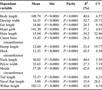
The ANOVA showed that site and parity had highly significant (P < 0.0001) effect on the total variation of all quantitative traits for female sample populations (Table 6). R 2 values ranged from 23.4 to 57.1 percent for hump length and heart girth, respectively. Coefficient of variability of female sample population explained by the model ranged from 4.92 percent for mouth circumference to 32.46 percent for horn length, respectively.
Level of significance of main effects for each of the variables and associated R 2 (%) values for the female sample population.

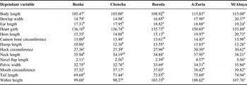
Pair-wise comparisons between sites (Table 7) showed significant (P < 0.0001) differences for all the quantitative traits. The highest least squares means for all measurements were recorded for sample cattle populations of Mirab-Abaya and Arbaminch-Zuria. As was observed on the male sample populations, relatively small measurements were observed for sample cattle populations at Bonke, Chencha and Boreda districts.
Least square means and pair wise comparisons between sites of body measurements (cm) for female population.

a,b,c,cb,dLeast squares means with different superscripts within the same row are significantly (P < 0.05) different.
Qualitative variations
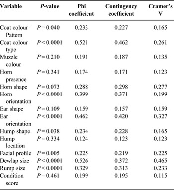
The chi-square tests for colour type, horn orientation, ear orientation, dewlap size and rump size were highly significant, compared with those for facial profile, colour pattern and hump shape. All other variables were not significant (P > 0.05). Associations of categorical variables with sites were much variable and ranged from 0.124 to 0.526 for hump location and dewlap size, respectively, using Phi coefficient; 0.123 for hump location, 0.462 for coat colour type using contingency coefficient, 0.115 for body condition score and 0.465 for dewlap size using Cramer's V (Table 8).
Chi-square tests and levels of association of sites with the categorical variables.

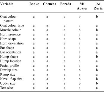
As presented in Table 8, variables other than colour pattern, muzzle colour, horn shape, hump shape, dewlap size, navel flap size and udder size did not make significant contributions in distinctly separating sample populations. Pair-wise comparisons made using the Bonferroni's correction grouped sample populations from Bonke, Chencha and Boreda into similar group and those from Arbaminch Zuria and Mirab Abaya into another category (Table 9).
Pair-wise comparisons of discrete variables using the Bonferroni's correction.

Sites with same letter on the same row are not significantly different at (P < 0.05).
Multivariate analysis
Discriminant analysis
The correct classification for female sample population into their site group ranged from 43.18 to 81.43 percent (Table 10). The overall average error count estimate was 36.85 percent for all observations and 63.15 percent of the samples were correctly classified. This higher error rates, for instance in Chencha and Arbaminch Zuria populations, indicate lower homogeneity of cattle populations in these samples and perhaps greater admixtures with adjacent cattle population types. For instance, populations from highland sites (Bonke, Chencha and Boreda) shared high number of cross-classifications with each other; this was also true for Arbaminch-Zuria and Mirab-Abaya. This also confirms that populations from these sites were phenotypically more closely related to each other.
Number of observations and percent classified (below) in different sites for female sample population using discriminant analysis.

In the case of males, the correct classifications ranged from 69.44 to 80.95 percent (Table 11). The overall percentage correctly classified for male sample populations was 74.89 percent. The highest correct classification percentage was observed for Mirab-Abaya in contrast to the least for samples from Arbaminch-Zuria district.
Number of observations and percent classified (below) in different sites for male sample population using discriminant analysis.

The overall correct classification rate (hit ratio) of 74.89 percent for males was higher than 63.15 percent for females. The first five quantitative variables that contributed more to group discrimination for female sample populations were muzzle circumference, neck length, navel flap length, heart girth and pelvic width. Ear length, hump length and tail length had least power in explaining variation between female populations across sites. For the male sample populations, the most significant discriminating quantitative variables were pelvic width, neck length, hump length, preputial sheath width and hock circumference.
Canonical discriminant analysis
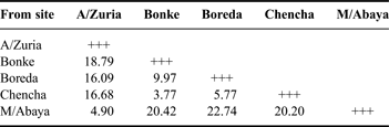
The pair-wise squared Mahalanobis' distances between sites for female sample populations were highly significant (P < 0.0001). This shows that female populations from each site have distinct and measurable group differences from other sampled populations. The shortest distance (3.77) was measured between Bonke and Chencha sites and the longest distance (22.74) was measured between M/Abaya and Boreda sites (Table 12). This indicates that sample populations from Bonke and Chencha, and perhaps Boreda as well, were not much different in the group quantitative features under consideration. The same is true in group differences between Arbaminch-Zuria and Mirab Abaya.
Squared Mahalanobis' distance between sites for the female sample populations.

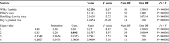
The univariate statistic testing the hypothesis that class means are equal shows that each variable is a highly significant (P < 0.0001) contributor to the total variation. The multivariate statistics for differences between the sites was also significant (P < 0.0001) in all of the four multivariate tests (Wilks' lambda, Pillai's trace, Hotelling–Lawley trace and Roy's greatest root for female sample population; Table 13). Wilks' lambda, the ratio of within-group variability to total variability on the discriminator variables, is an inverse measure of the importance of the discriminant functions. The Wilks' lambda test for the female sample populations was 0.223 (Table 13). This shows that most (77.77 percent) of the variability in the discriminator variables was because of differences between populations rather than variation within populations.
Multivariate statistics and F approximations for female population.

The procedure for canonical discriminant analysis extracted four canonical variates for female sample populations, of which the first two canonical variates (can1 and can2) accounted for about 89.01 percent of the total variation (Table 13). The rest two canonical variates account for only 10.09 percent of the total variance. The plot of the first two canonical variates (can1 and can2) shows that can1 best separated female sample populations of the two sites (Arbaminch-Zuria and Mirab-Abaya, lowland types), from the other three sites (highland types). The second canonical variate further separated sample populations at Bonke from those at Boreda, with those at Chencha falling in between the two. Based on these results, the CANDISC procedure of SAS (2002) classified female sample populations into two distinct populations – highland and lowland types.
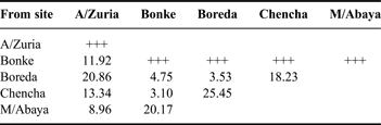
In the case of male sample populations, the squared Mahalanobis' distance between the sites was slightly higher than it was for female populations. The shortest distance (3.10) was observed between Bonke and Chencha sites and the longest distance was between Boreda and Mirab-Abaya sites with a value of 25.45 standard units (Table 14). The distances expressed here between sample populations are due to distinct phenotypic differences between populations for quantitative traits. Both univariate and multivariate tests generated from canonical discriminant analysis confirmed the existence of highly significant differences between male sample populations between highland sites (Bonke, Chencha and Boreda) and lowland sites (Arbaminch-zuria and Mirab-Abaya).
Squared Mahalanobis distance between sites for the male sample populations.

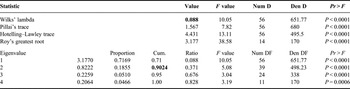
Four canonical variates were also extracted from canonical discriminant analysis on the male sample populations as was the case for female populations. The first two canonical variates (can1 and can2) altogether explained 90.24 percent of the total variation, with the remaining two accounting for only 9.76 percent of the total variation (Table 15). Based on the coefficients of the first canonical discriminant function (can 1), two clear groups of cattle populations of the study area emerged: highland types (Bonke, Chencha and Boreda) and lowland types (Arbaminch-Zuria and Mirab-Abaya).
Multivariate statistics and F approximations of male population.

The plot of the first two canonical variates showed to some extent similar pattern with those of female populations. In contrast with female populations, the first canonical variate (can1) separated sample population of Arbaminch-Zuria and Mirab-Abaya from the other three sites that appeared bundled together. The second canonical variate (can2) further differentiated male sample populations of Bonke and Arbaminch-Zuria from Bonke and Mirab-Abaya, again Chencha appearing as an intermediate. These discriminations are in fact stronger than the outcomes based on the female samples.
Stepwise discriminant analysis
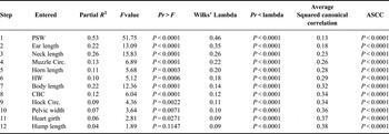
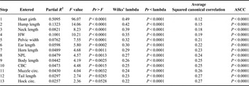
All 14 quantitative variables for both sexes were separately subjected to the STEPDISC procedure of SAS (2002) and 13 variables for females and 12 variables for males were identified as best discriminating variables on Stepwise selection summary. Wilks' lambda test shows that all the traits considered were highly significant (P < 0.0001) contributors to discrimination of the total population into separate groups. The variables with the highest discriminating powers on the male population were sheath width, ear length, neck length, muzzle circumference, horn length, wither height, body length, canon bone circumference, hock circumference, pelvic width, heart girth and hump length (Table 16). Dewlap width and tail length did not have significant discriminating powers on the male population and were removed.
Stepwise selection summary table for male populations.

Note: PSW = perputial sheath width; CBC = canon bone circumference; HW = height at withers; Circ. = circumference.
Similarly, best variables that discriminated the sample female population were heart girth, hump length, neck length, wither height and pelvic width (Table 17). Hump length was weak in separating female sample population and was removed.
Stepwise selection summary table for female populations.

Note: NPL = navel flap length; CBC = canon bone circumference; HW = height at withers; Circ. = circumference.
Non-parametric discriminant analysis
The overall hit rate obtained from non-parametric discriminant classification was 93.6 percent (Table 18). This indicates that categorical variables are also important in classifying the populations in phenotypically distinct groups. Wuletaw (Reference Wuletaw2004) reported similarly lower error rate of 2 percent, in contrast to 47.5 percent and 22.8 percent by Getachew (Reference Getachew2006) and Tadesse (Reference Tadesse2005), respectively for similar categorical variables.
Number of observations and percent classified (below in the bracket) into site using non-parametric discriminant for both sample populations.

Description of the identified cattle types
Results from focus group discussions, field observations on discrete phenotypic features and univariate as well as multivariate analyses revealed that there are two major cattle types/strains identified in the study area. These are termed as Gamo highland and Gamo lowland populations taking into account their phenotypic differences as well as their geographic distribution. Both have well-developed humps and express zebu characteristics and hence both could be considered to be zebu-type cattle.
Gamo highland sub-population
These cattle were known by their high adaptability behaviour to highland production environment which is characterized by a cold climatic condition, long wet season, undulated topographic feature and high altitude above 2500 m asl. Crop residue, natural vegetation and Enset were major sources of feedstuffs. Animals are housed together with humans. They are multi-purpose animals and kept mainly for milk, manure, cash, traction and meat.
Key informants explained that highland cattle types are not known by general name in the community. However, owners give local names depending on coat colour type. However, some owners give traditional names to identify their animals from the herd. No clear origin information was available and farmers believe that they may have evolved from adjacent highland areas through local marketing channels. They are also well adapted to highland districts of the zone and other neighbouring areas.
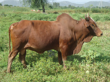
Their physical distinctness is explained by small compact body size, mainly small dewlap size, small erect and thoracic hump, straight and lateral oriented ear, and proportionate head with mainly straight facial profile. Few animals were recorded with concave facial profiles. Major horn orientation recorded was upward and some had tips pointing lateral. Muzzle colour almost not pigmented and a few were found with black pigmentation. Tails were medium and reach hock bone. Spotted/pied mixture of black with other colours (red, grey and white) was common. Rump shape is mainly sloping and some are flat and roofy. Females have small to medium udder size; mainly small navel flap. Medium teat size for female animals and medium sheath size for male animals was recorded.
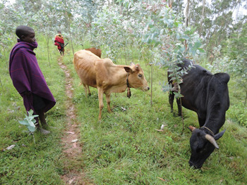
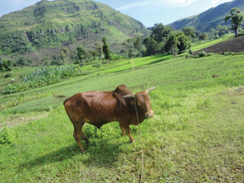
According to local sources, the total indigenous cattle population of all highland districts is estimated to be about 723 thousand heads. The population size is reportedly declining. Diminishing grazing land, poor extension service and poor breeding activities (indiscriminate cross breeding with Holstein bulls and traditional selection focused on high production) were suggested to have contributed to the reduction in population size (Figures 1 and 2).
Breeding cow from Bonke site.

Breeding bull from Boreda site.

Gamo lowland sub-population
This type of cattle adapts to the hotter climatic conditions of lower altitude areas with long dry season and mainly plain topography. Some of these areas are infested with tsetse flies. The altitude is below 1500 m. The dominant production system is livestock–crop mixed, and communal grazing on natural bushy pastures is common. These cattle are not known by any local name. It was suggested in the focus group discussions that these cattle may be either related to or originated from lowland pastoral areas of Borana and South Omo.
Major production functions of the cattle include milk, draft and meat. Their roles in generating cash and meeting social obligations are also recognized. The current total estimated population of lowland cattle is 437 000, and this is known to be declining. Prevalence of various diseases and heavy parasitic infestations, expansion of crop farming at the expense of pastures, seasonal feed scarcity and lack of genetic improvement programme of existing local cattle are the major constraints identified.
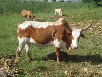
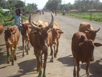
Peculiar characteristics of this zebu type of cattle are mainly plain coat colour and with some being pied and spotted. Majority are plain dark/light red and fawn colour. Red and white mixtures were dominant and rarely white and black spotted were observed. Hump is located mainly at thoracic position and mostly dropping for adult males. However, there were also some cattle with cervico-thoracic hump. They were medium to large in body size with well-developed dewlap, medium neck length, wide muzzle circumference mostly with no pigmentation. Tails are long and thin, and pelvic bone is wide. In addition, majority of female animals were identified by their medium navel flap length and large, squarely arranged medium teat size and well-developed medium-sized udder. They are medium to long horned. About 92.5 percent were horned with curve shape and oriented upward. Ears are long, straight edged (81.0 percent) and laterally oriented (72.6 percent). Sample pictures from lowland cattle sub-population are presented in Figures 3 to 5.
Breeding bull from Arba-Minch Zuria district.

Adult male animal from Mirab-Abaya district.

Breeding female herd from Arba-Minch Zuria district.

Conclusions
ANOVA on continuous variables showed significant (P < 0.0001) differences between sites, both for females and males populations. Chi-square tests for categorical variables between sites showed highly significant (P < 0.0001) differences between sites for most of the variables. Based on results of the discriminant analysis, sample populations were classified into two – highland and lowland cattle populations, which were corroborated by results of the canonical discriminant analysis. Results of the step-wise discriminant analysis also confirmed the distinct aggregate phenotypic differences between highland- and lowland-type cattle populations. These statistical results confirmed outcomes of the focus group discussions in which consensus was built on clear differences in body form and size between cattle populations of the highland and lowland areas of Gamo Goffa Zone.
Based on these results, the hypothesis that the local cattle populations of Gamo Goffa zone are phenotypically homogenous is rejected. Therefore, the highland- and lowland-type of cattle are significantly different in their phenotypic characteristics that merit further in-depth phenotypic and genetic studies not only to investigate their breed identity but also to lay out the basis for sustainable utilization and improvement of this indigenous genetic resource.