

Introduction
Chile has displayed the most successful economic growth in Latin America during the last 25 years with an average growth rate of approximately 5 per cent. This sustained growth has led to a dramatic reduction in poverty rates from 40 per cent in 1990 to 18 per cent in 2003, although inequality has remained persistently high.Footnote 1 On the basis of cross-sectional data, Chile is considered a successful case of poverty reduction and targeted public policies in Latin America. The surveys undertaken for the Encuesta Nacional de Caracterización Socioeconómica (CASEN) and census data have provided evidence of the increase in the wellbeing of Chilean households during the last decade.Footnote 2 However, other surveys (such as those undertaken by the Centro de Estudios Públicos (CEP) and Futuro) have indicated that Chilean households feel unprotected in different ways. They reported that they face significant labour instability, lack of proper health insurance, poor access to quality education, and uncertainty about social security programmes. In other words, in spite of the documented increases in welfare that have taken place, many Chilean households consider themselves vulnerable.
The main objective of this paper is to study the dynamic aspects of poverty in Chile. Using panel (longitudinal) data from the CASEN database from 1996 and 2001, we provide new evidence on the characteristics and determinants of poverty in Chile. Repeated observations of panel data identify poverty both as a temporary condition, presumed to be caused by a negative income shock, and as a systematic or chronic situation deriving from meagre human and physical assets. This is especially important in view of the period covered by the panel data, as significant economic and social changes occurred in Chile between 1996 and 2001. The Asian financial crisis affected the Chilean economy, reducing investment and growth and increasing unemployment. This context makes it all the more interesting to analyse the dynamics of income and poverty, the determinants of income changes, and the groups which were more intensely affected by economic recession.
In this paper we investigate the direct factors behind changes in poverty status and the characteristics associated with a higher probability of falling into this condition, as well as those related to leaving it behind. The poverty line defined here is based on the cost of a nutritionally adequate diet measured as a minimum bundle, the composition of which is given by the Economic Commission for Latin America and the Caribbean. The bundle satisfies the minimum individual requirements in terms of calories and proteins advised by the World Health Organisation and the Food and Agriculture Organisation. This is the official measure of the poverty line for Chile. It should be noted, however, that the standard procedure of estimating levels of poverty by using a fixed poverty line ignores the significance of regional heterogeneity in prices, and economies and equivalence to scale at the family level.
From a welfare standpoint, one might be interested in evaluating poverty dynamics using several different possible poverty lines. For this reason the results are estimated for different thresholds of poverty. Thus, we undertake simulations for a broad range of poverty lines (starting with the standard definition) and emphasise the robustness of most of the results. The findings presented show the usefulness of this simple procedure, which provides a clearer picture of poverty and its characteristics.Footnote 3
We follow recent literature by dividing the poor into two groups according to their poverty status in time. We define transient poverty as the proportion of households which were poor in either 1996 or 2001, but not both, and chronic poverty as the proportion which remains poor in both periods. Since we have only two observations in time, this distinction allows us to fix an upper bound on the number of households which are systematically poor and a lower bound on the number of households which experience poverty in a transitory manner.
Using these definitions and the available data, the evidence indicates that at least half of all poverty in Chile at a given moment in time is transient in nature, and that this component remains stable as the poverty line rises, while the chronic portion rises steadily. Static poverty fell from 22 per cent in 1996 to 18 per cent in 2001, but more than 34 per cent of the population was poor at one of these points, establishing the broader reach of this dimension of poverty. The data indicates that 46 per cent of the poor in 2001 had not been poor in 1996.Footnote 4 Moreover, the ‘new poor’ in 2001 came from all deciles of the population, although only 14 per cent of them had been in the top half of the income distribution in 1996.
As one would expect, labour dynamics seem to be the main driving force explaining income movements that lead to entry into and exit from poverty, while changes in household size, subsidies, and other sources of income seem to be less important in explaining the flux in poverty status. An interesting finding is that in households which left poverty in response to a rise in income from their labour, the spouse was twice as likely, and other members were three times as likely, to get a job, as the household head.
There is evidence that if the household head suffered from any major health problems between 1996 and 2001, the probability of exiting poverty was significantly reduced. Households with a higher number of children under the age of 15 have a higher probability of falling into poverty, and a lower probability of exiting it. Household heads who work in the public sector have lower predicted income levels, but also a lower probability of falling into poverty. The opposite is true for households which own businesses or where members are self-employed or independent workers. Finally, we find that technical education is statistically associated with a higher probability of exiting – and a reduced risk of entry into – poverty.
These results are important for several reasons and have direct policy implications. The apparent Chilean success in reducing poverty is challenged. A look at poverty dynamics points to the fact that many more households experience transient poverty, which has obvious adverse welfare effects if credit markets are incomplete and consumption smoothing is not possible. This is not to say that things are not better than twenty years ago, but it highlights the fact Chile is still a poor country.
From a policy point of view, the 9 per cent of households which remain poor after five years justifies social programmes such as Chile Solidario which focus on the extremely poor. However, poverty reduction strategies will have to pay attention not only to those who are currently poor, but also to non-poor households which might be at risk of falling into poverty at some point in the future.
The significance of labour dynamics underlines the importance of policies such as the new unemployment insurance system, and suggests the need to expand its relative importance in the design of social safety nets in the future.Footnote 5 The larger role found for the labour participation of other members of the household in helping them to exit poverty leads to the obvious conclusion that facilitating this process for poor households, by offering support such as public child care and job training, would lead to less chronic poverty and static poverty. The road out of poverty is fragile, and poor households need adequate health coverage and insurance to protect them from adverse shocks that permanently impair their capacity to generate income.
Empirical Evidence
The empirical evidence on poverty dynamics reviewed by Bob Baulch and John Hoddinott in 2000, and the later work undertaken at the Chronic Poverty Research Centre, has emphasised that there are different types of poverty, and that understanding their underlying characteristics is extremely valuable for policy design.Footnote 6
Jyotsna Jalan and Martin Ravallion showed in 1998 that in rural China transient and chronic poverty are explained by different variables.Footnote 7 One possible theory is that chronic poverty is the result of having insufficient productive capital, while transient poverty is associated with random shocks with which the household is unable to cope. According to this argument policies aimed at resolving chronic poverty should concentrate on increasing the capital that these households possess, while policies aimed at reducing transient poverty should focus on mechanisms that allow families to smooth consumption, such as better access to capital markets and social insurance.Footnote 8
Baulch and Hoddinott show that, in general, the transitory component of poverty has been found to be relatively larger than the chronic part. One extreme case is that of rural India (1975–1984) where 80 per cent of the population were defined as poor; however, more than 60 per cent of the total population suffered from transient poverty, while only 20 per cent experienced chronic poverty.Footnote 9 The 2005 report, of the Chronic Poverty Research Centre in Manchester, finds that in Latin America chronic poverty is between 30 and 40 per cent of total poverty.Footnote 10
The literature reports four principal sets of findings regarding poverty dynamics in developing countries. First, chronic and transient poverty exist alongside each other, but are distinct. Second, they have different determinants, and the transient component is usually larger than the chronic component. Third, changes in the returns to households' capital are an important source of income growth. Finally, changes that are apparently transient can lead to permanent effects.
In Chile, trustworthy and nationally representative studies based on cross section data have existed since 1987, when the first CASEN survey was completed. According to a group of economists based in Chile, writing in 2001, the main determinants of poverty during the 1990s were low wages, low labour participation rates, and the large number of people in each household.Footnote 11 Nonetheless, as Julie Litchfield has shown, between 1987 and 1998 poverty was reduced by half.Footnote 12
Other studies performed by the World Bank, the Inter-American Development Bank and the United Nations Development Programme have presented evidence of the relationship between gender status and poverty levels. Households with female heads and low human capital are significantly poorer than their male counterparts with similar characteristics. Poverty also has a regional component. Throughout Chile's development process, certain sectors have experienced less poverty reduction, especially in the late 1990s. Rural sectors with low human capital and those located in areas of lower growth have shown difficulties in raising their standard of living at the same rate as the rest of the country. Finally, it has been shown that the opening of the economy to international trade has had an important impact on poverty reduction due to higher economic growth.Footnote 13
The first studies of poverty dynamics in Chile were undertaken by Julie Litchfield and Christopher Scott.Footnote 14 Both papers made use of a panel dataset containing approximately 200 rural households with observations dating from 1968 and 1986.Footnote 15 The authors conclude that poverty reduction was mainly explained by pensions and other transfers. They also found that there was remarkably low social mobility in the period under consideration.Footnote 16
Methodology
Let us assume that households own a heterogeneous set of assets: physical, financial, human capital, etc.. The income of households will then depend on the use given to these assets and the return that they command on the market. Once the household has assigned its assets to different activities, other events intervene in the form of shocks. These shocks may be general and affect all households, for example a war or an economic recession, or they may be specific to each household in the form of occurrences such as layoffs, sickness or accidents.
Here one can distinguish two possible types of poverty: chronic and transient. Chronic poverty might be associated with households with insufficient assets, while transient poverty might be explained mainly by shocks. This distinction would imply that policies aimed at reducing poverty should take into account the different aspects of each of these types of poverty. While the logical separation to be made in policy between long-term asset building and short-term social protection is still disputed, we believe that the evidence presented in this paper supports the idea that using different policy instruments to address different types of poverty will have a more significant effect on poverty overall.Footnote 17
This paper addresses the conceptual problem in three steps. First, attention is given to movements in and out of poverty, measuring the relative size of each type. In this way, given the two observations that are available, households can be divided into four groups depending on their dynamic poverty status: those which are always poor, those which fall into poverty, those which leave poverty, and those which are never poor. Households which are poor in 1996 and remain so five years later are considered chronically poor. Those which experience poverty in only one moment in time (one observation) are interpreted as transiently poor, while the residue is simply not poor.
Second, we examine the direct causes that bring about the change in poverty status by decomposing the change in income into its different sources. Our interest is in household per capita income, which includes all labour income from the household head and other members, monetary subsidies and transfers from the government and private institutions, and imputed rent.Footnote 18 The change in income can thus be decomposed into changes in labour income, other monetary incomes, and the change in number of people in the household. A similar procedure was undertaken by Woolard and Klasen for South Africa.Footnote 19
Finally, after identifying the direct causes of the change in status, in order to examine the factors that influence the ex-ante probability of falling into poverty, a dependent variable is defined equal to 1 if the household was not poor in 1996 but poor in 2001. The right hand side variables are the initial conditions of the household in 1996. Similarly, in order to examine the factors that influence the ex-ante probability of exiting (staying in) poverty, the dependent variable takes the value 1 if the household is poor in 1996 and not poor in 2001. The right hand side variables are the initial conditions of the household in 1996.
The robustness of the results was examined using a broad range of poverty lines. We find that some variables are not robust, while others which are not significant in the baseline case are significant for most other poverty lines.
The Variables
As already discussed, transient and chronic poverty may be explained by different variables. On the one hand, we might assume that chronic poverty is related to low productive capital, while transient poverty can be associated with random shocks with which the household is unable to deal. Neil McCulloch and Bob Baulch suggest that the determinants of income and poverty dynamics of a household should include a vector of variables that approximate the characteristics of the surrounding environment, the different assets that the household owns, as well as the composition of the household and any observable shocks.Footnote 20
The geographical characteristics of the household's environment affect the productivity of its assets, as do its access to public services and transport. In our estimates a dummy variable that defines a household as rural or urban was included, as well as variables that identify each region of the country included in the data set.Footnote 21
Human capital and the total available workforce of the household are used to measure household assets. Human capital is proxied by the education of the household head, as well as the average educational level of the other adult members of the family. Additionally variables that describe the economic sector where the household head works were included. The type of contractual agreement that the households' workers have with their employers was also included in order to proxy the quality of their jobs.Footnote 22 Although the data available does not include information on a household's financial or physical assets, it does provide information on home ownership. This is used as a proxy for savings and physical capital. Social capital was proxied by a dummy variable defined as equal to 1, if the household has no one to help them in a time of need, as defined in the survey, and 0 otherwise.Footnote 23
In order to measure the demographic composition of the household, the variables were defined as the number of individuals in different age categories.Footnote 24 The dependency ratio was also calculated as the ratio between the number of workers and total family members. Finally, the survey data provides a measure of adverse health shocks.Footnote 25 A dummy variable is defined as 1 if the household head reported a serious illness during the period between 1996 and 2001, and 0 otherwise.
Data
The CASEN household survey is undertaken by the Ministerio de Planificación and is representative at a regional and national level. Its objective is to describe socioeconomic conditions and evaluate social policies. The survey is carried out at the household level, as well as the personal level. Information is collected to describe income, educational characteristics, access to housing, health services and social programmes, as well as the labour force status of all household members.
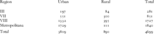
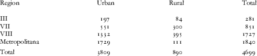
The CASEN 1996–2001 panel is the first database in Chile that follows a representative sample of the national population over a period of time. The potential sample for the panel survey is made up of all those households which were interviewed during the 1996 CASEN cross-section survey and who live in the III, VII, VIII and Metropolitan regions.Footnote 26
The total number of households surveyed was 4,700 out of the 5,326 selected. Of these, 4,042 were also surveyed in 2001, while the remainder were new households that had been formed from the original households surveyed in 1996. Our unit of analysis is the household and the income variable used is per capita income, where income is defined as total monetary available income plus imputed rent income. This is standard procedure in calculating poverty in Chile.Footnote 27
Attrition and Measurement Error
Two common potential sources of bias in panel data are attrition and measurement error.Footnote 28 The attrition rate of the CASEN panel was 28.1 per cent after five years which is equivalent to an annual attrition rate of approximately 6 per cent. This is relatively low when compared to other panels.Footnote 29 Measurement error is also a potential problem with panel data, and may be especially important when studying income dynamics. With the information we have, it is not possible to know the amount of measurement error in the data, but we analyse and limit this problem in three ways.
The first way is to limit measurement error in reported labour income by estimating a standard wage equation and eliminating observations that have more than two standard deviations from the predicted income of that observation.Footnote 30 Using this new labour income series we recalculate our transition matrix and regression analysis.Footnote 31 These results are presented in the Appendix. Although one might doubt the source of outliers eliminated from the data, it is by no means clear that these extreme deviations are due to measurement error.
The second way is to aggregate data at the household level and avoid some individual-level measurement error. The original data comes at individual and household level. We choose to construct household level variables from the individual level data so as eliminate (average out) some of the measurement error that would occur using aggregate households as the unit of investigation.
The third way that we try to limit measurement error is by using initial conditions, X1996 in our regression instead of change in the variables X2001 – X1996. We are thus not vulnerable to compounding measurement error in these variables, though there may still be initial measurement error and compounded measurement error in the variables that measure income. An exploratory way in which we assess the extent of measurement error present in our income variables is by observing how household assets change when they experience different income trajectories. We would expect assets to be partially correlated to income and find that households which fall into poverty would have sold part of their assets in an attempt to smooth consumption. The survey provides information on home ownership, and when tracking this variable we find that 79 per cent of households who owned a second home – and fell into poverty – lost it, while 20 per cent of those who owned a single home and fell into poverty lost it. This is in line with what one would expect if the household suffered a negative trajectory.
We conclude that this evidence, while exploratory in nature, bolsters the argument that the movements into poverty are not purely measurement error and are associated with real changes in income.
Results
Transition matrix analysis
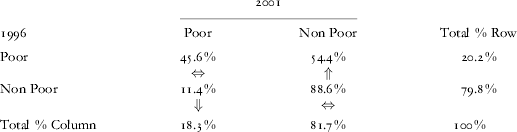
Absolute mobility with respect to entering and exiting poverty is characterised by the transition matrix presented in Table 1. The evidence shows that more than half of all poor households (54 per cent) in 1996 were not poor in 2001. The transition matrix also shows, however, that 11.4 per cent of households which were not poor in 1996 fell into poverty in 2001; the ‘new poor’ in 2001 thus actually account for 46 per cent of all poor at that time.
Transition Matrix
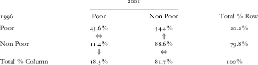
Note: The rows indicate how poor and non-poor households in 1996 are distributed in 2001. Of the 20 per cent poor households in 1996, 45 per cent of them remained poor in 2001, while 11 per cent of the non-poor in 1996 fell into poverty and account for 46 per cent of all poor in 2001. This implies that chronic and transient poverty were 9.2 per cent and 20.1 per cent respectively.
Source: Authors' calculations from CASEN panel data, 1996–2001.
Transient poverty can be calculated from the transition matrix in Table 1 as the sum of those who exit and enter poverty, while chronic poverty is simply the proportion of households which remain poor in both periods. We find that between 1996 and 2001, 20.1 per cent (54.4×20.2+11.4×79.8) of the population was transiently poor, and chronic poverty was 9.2 per cent (45.6×20.2). This implies that more than half of all poor households observed at a moment in time are indeed transiently poor, and that 30 per cent of the population had income under the poverty line at some point during the two periods observed.
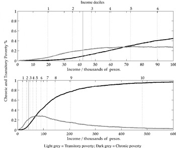
The results above are directly associated with a specific poverty line. We next analyse the sensitivity of both chronic and transient poverty to changes in the poverty line to find how robust these results are. While chronic poverty should be increasing monotonically with the poverty line, transient poverty need not follow this behaviour. To examine this possibility, the transition matrix was calculated for a wide range of poverty lines and the decomposition of poverty in both years is presented in Figure 1.
Transition Matrix for Different Poverty Lines. Note: These graphs show the evolution of chronic (the dark line) and transient poverty (the lighter line) as the poverty line changes (the X-axis). The actual poverty line is approximately Ch$42,000 per capita (the dark vertical line). The light vertical lines denote the average income of the decile noted at the top of the graph.

The top plot in Figure 1 presents the evolution of chronic poverty (the dark line) and transient poverty (the lighter line) for poverty lines ranging from Ch$0 to Ch$100,000 per capita, where the current poverty line is approximately Ch$43,000 (approximately US$75) per capita (the dark vertical line).Footnote 32 The light vertical lines denote the mean income of the decile noted at the top of the graph. The bottom graph repeats the same exercise for a larger set of poverty lines. One can see that while chronic poverty increases systematically, transient poverty levels out between deciles 2 and 7, then falls, where the income distribution is quite smooth, as can be seen in Figure 2. We can conclude from this analysis that transient poverty is around 20 per cent for a large set of proximate poverty lines and that chronic poverty rises by 0.7 per cent for every 1,000 pesos increase in the poverty line.Footnote 33
Logit Regression Sensibility to the Poverty Line.

Direct causes of the change in poverty status
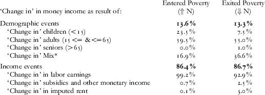
The change in income per capita that has brought about the reversal in poverty status can be separated into several components. Changes in income per capita can be divided into changes in the numerator (incomes) and changes in the denominator (number of people). The numerator can be further divided into the labour income of the household head and that of other members, subsidies and transfers, and imputed rent. Table 2 presents the decomposition of each of the main reasons why a household changed their poverty status.
Main Event Associated with the Reversal of Poverty Status (% of households)
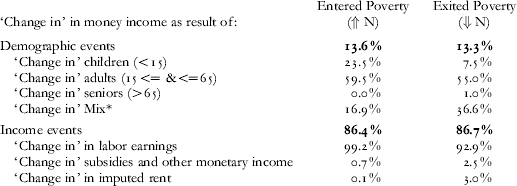
Note: The main event was determined as the largest change leading to the reversal in status. So if all categories contributed to the change in income, the largest would be attributed as the main event. Note that labour dynamics seem to be the fundamental issue explaining poverty dynamics.
* Mix indicates that not one category is responsible for more than 50% in the change in N.
Source: Authors' calculations from CASEN panel data, 1996–2001.
When compared to the results for South Africa, found in Woolard and Klasen, we find a smaller demographic influence and a larger labour effect in Chile. While in South Africa 27 per cent and 23 per cent of changes were due to demographic events, only 14 per cent and 13 per cent were so caused in Chile.Footnote 34
Table 3 shows the change in the labour participation of the members of households where labour income explained the change in poverty status. While the loss of employment of any family member is relevant for falling into poverty, it should be noted that the participation of the spouse and other members of the family plays an important part in explaining household exit from poverty.
Labour Status of Household Members (% of households)


* HH abbreviates Household Head.
** ‘Others’ implies other members of the household excluding the HH and spouse.
Note: This table presents labour participation in households where labour income was determined to be the main source explaining the change in poverty status in Table 2. Notice that the employment of the spouse and other members of the household seem to be very important for leaving poverty behind.
Source: Authors' calculations from CASEN panel data, 1996–2001.
Determinants of poverty dynamics
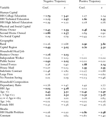
This section presents evidence on the determinants of poverty dynamics in Chile. The factors that explain the ex-ante probability of entry and exit from poverty are examined using logistic regressions based on the conditions in the base year (1996), and study the correlation of household variables to the negative (falling into poverty) and positive (exiting poverty) trajectories.
The results are shown in Table 4. The dependent variable takes the value of 1 if the household experiences a change in its condition and 0 otherwise. The positive trajectory refers to changing from poor to non-poor, while the negative trajectory refers to the change from non-poor to poor. The right hand side variables are presented using 1996 levels.
Determinants of Poverty Dynamics

Note: Negative and Positive Trajectory Logit Estimations were calculated using 2,955 and 1,085 observations respectively. Pseudo R2=0.12 in each case. The HH (Household Head) Business Owner dummy variable was a perfect predictor of the positive trajectory and was dropped (1 observation) from the estimation.
As expected, education is a relevant characteristic associated with both positive and negative trajectories. However, we find it is less important than one might have thought in view of the international evidence presented earlier in this paper. An interesting result is the absence of a positive effect of high school and college education on the probability of experiencing a positive trajectory (leaving poverty behind). On the other hand, more educated households do have a smaller chance of falling into poverty. Technical education, however, serves both to raise the probability of exiting, and to lower the probability of entering poverty. This asymmetry suggests that technical education provides households with a type of insurance against poverty.Footnote 35
We find that households in the Metropolitan Region fared better than their counterparts in other regions. It is interesting to note that rural households left poverty more frequently and thus the geographic regions which fared worst were the urban areas outside Santiago.
The sector of the economy in which the household head is employed is shown to be a determining factor that explains households' future income paths. Workers in the armed forces as well as those employed as domestic servants or maids are found to have a higher probability of exiting poverty. Public sector workers are also shown to be less likely to become poor.Footnote 36
The evidence also suggests that the demographic composition of the household is an important determinant of poverty dynamics. The household's point in the life cycle, as measured by the age of the household head, affects the probability of falling into poverty. In other words, younger households are more vulnerable. Additionally, a household with a higher number of children under the age of 15 faces a reduced probability of exiting poverty.
As expected, the results also show that families that own another house besides the one they live in have a higher probability of exiting and a lower probability of entering poverty. This may be due to the fact that if the household owns another house, it probably has other assets not captured by the survey; such households are better able to overcome adverse shocks, making them only transiently rather than chronically poor.
It is relevant to note that female household heads were neither more nor less likely to leave or enter poverty than male household heads.
Finally, household heads who have reported an important health problem, experience more difficulties leaving poverty. This suggests that low income homes do not have an effective way of dealing with medical problems. It is relevant to note that the health problem variable takes the value of 1 if the household head had to be hospitalised at any point between the survey in 1996 and the survey in 2001. With that in mind, the significance of this variable also suggests that health problems have permanent effects on income for initially poor households. Non-poor households, however, seem not to have the same problem when confronted by negative health shocks.Footnote 37
Robustness of the poverty line
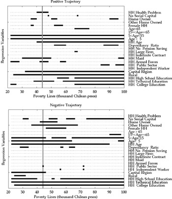
The objective of the following exercise is to take direct account of the fact that the parameters of the regressions are dependent on the poverty line used and that the results may be specific to a particular poverty line. We recalculate poverty status and trajectories for a large set of poverty lines, and proceed to estimate each regression, recording the significance of the parameters in each case. Figure 2 summarises the results from the simulation. The regression variables are listed on the right of the Y-axis and the X-axis shows the poverty line used to estimate the model. A thick line indicates that the variable was significant and a dotted line means that it was not significant.
The top plot in Figure 2 shows the positive trajectory regression and the bottom plot shows the negative trajectory regression. The actual poverty line is plotted with a thick vertical grey line and denotes the regressions shown in Table 4.
For the positive trajectory, namely being poor in 1996 and exiting poverty in 2001, we can see that the health problem variable is relevant only for a set of poverty lines between Ch$40,000 and Ch$50,000 per capita, which is roughly the second-third decile of the population.
The household composition variables are very robust and are always significant independently of the poverty line. This is in line with other evidence in the literature, but it is worth noting that having more children affects poverty not only because it means dividing total household income between more people, but because they are also associated with a lower probability of leaving poverty.
Regarding other variables, we see that household heads who worked as a maid, or in the armed forces were also significant for several poverty lines, but stop being relevant once the poverty line goes up 10 per cent. Geographical location seems to be very relevant as rural households systematically fare better than their urban counterparts, as do households in the metropolitan region. Finally we can see that although educational variables like college and high school education were not significantly associated with exiting poverty at the current official poverty line, they are significant when the model is estimated with a higher poverty line.
For the negative trajectory, that is households that were non-poor in 1996 and had entered poverty in 2001, we can see that the lack of social capital seems to be more relevant than initially thought, since it is significant for many poverty lines but not the current one. Home ownership is important, but owning a second home is even more robust, since it is relevant for a larger set of poverty lines. Household composition is again very relevant, independently of the poverty line used.
Using the current poverty line we find that household heads who work in the public sector are less likely to fall into poverty, but this result vanishes after only small changes in the poverty line, whether up or down. This result thus appears not to be particularly robust.
Geographical location in this case is significant for the current poverty line but a small increase in the poverty line reduces its importance. Finally, educational variables are significant for most poverty lines. High school education, which was not relevant for avoiding poverty in the model using the current official poverty line, is relevant for many other poverty lines.
As a result of simulating the results under different poverty lines we have found that social capital and high school education are more relevant than the initial results would indicate using only the current official poverty line. We also see that the earlier result, which finds household heads working in the public sector to be less vulnerable, is not very robust.
Conclusions
Using panel data, this article has examined the dynamics of poverty in Chile and the robustness of these results to changes in the poverty line. The evidence is based on three complementary strategies. First, poverty in Chile is decomposed into transitory and chronic components. Second, the direct causes of the change in poverty status are identified. Finally, the factors underlying poverty dynamics in Chile are considered for a wide range of poverty lines.
The evidence indicates that 54 per cent of the poor in 1996 were not poor in 2001, while 48 per cent of the poor in 2001 were not poor in 1996. Thus the transient component of poverty amounts to 24 per cent of the sample households that were poor in 1996 but not in 2001. The chronically poor consist of 10 per cent of the population: households which were poor in both 1996 and 2001. When we change the poverty line we find chronic poverty rising by 0.7 per cent for every Ch$1000 by which household income deteriorates while transient poverty remains roughly the same. In this way, while transient poverty is twice the amount of chronic poverty, the proportion of total poverty for which it accounts falls when the poverty line rises.
Labour dynamics is the main factor driving entry to and exit from poverty, and demographic factors and other sources of income seem not to be very relevant. A detailed examination of the variables associated with the probability of entering and exiting poverty has shown that health shocks to the household head seem to be a significant obstacle to leaving poverty, although this is not true for households with higher incomes. The number of children under the age of 15 negatively affects the probability of leaving poverty, and makes falling into poverty easier. The educational level of the household head reduces the risk of becoming poor, but does not significantly help – with the exception of technical education – those already poor to exit this state for the current poverty line. Education would thus seem to provide an insurance function in this dynamic context.
Households that own their own home or a second home are less likely to fall into poverty. We find that household heads who work in the Armed Forces or as housemaids are more likely to exit poverty.
Finally when simulating our results under different poverty lines, we find that several of our results change. Some variables were not robust to small changes in the poverty line, while others were significant for a large proportion of poverty lines but not for the current official one. As a result of simulating the results under different poverty lines we have found that social capital and high school education are more relevant than at first thought when using only the current poverty line. We also find that the earlier result, establishing that household heads working in the public sector are less vulnerable, is not very robust. This highlights the relevance of carrying out such a simulation for robustness and to account explicitly for the fact that the poverty line is an arbitrary threshold.
In summary, we find that this dynamic approach adds new evidence to the understanding of poverty in Chile, and highlights the wide range of future challenges for social policy. While Chile has been successful in reducing poverty levels in the past, an inspection of the dynamics of poverty points to the fact that many more households experience transient poverty, and that further headway in poverty reduction will need to address these dynamic features of poverty.
From a policy perspective, the significant group (9 per cent) of households which remains poor after five years provides evidence that justifies social programmes such as Chile Solidario which focus on the extremely poor. However, poverty reduction strategies will have to pay attention not only to those who are currently poor, but also to non-poor households which might be at risk of falling into poverty at some point in time in the future.
This evidence, of the importance of labour dynamics, supports the relevance of policies such as the new unemployment insurance and points to the need to expand its role in the design of future social safety nets. The significance of labour participation of other household members in assisting households exit from poverty leads to the obvious conclusion that facilitating this process for poor households – by offering facilities such as public child care or job training – would lead to less chronic and static poverty. The road out of poverty is fragile, and poor households need adequate health coverage and insurance to protect them from adverse shocks that permanently impair their capacity to generate income. New initiatives to improve the public health system (such as the current government's Plan Auge, which aims to protect an important part of the population from health problems) would coincide with the empirical evidence found in this study.
Appendix
Wage regression and measurement error
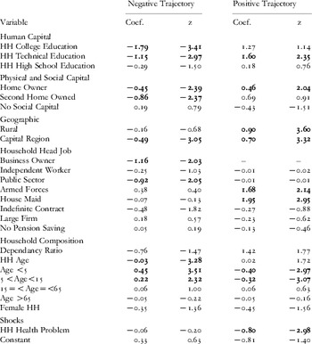
The following regressions show the results of repeating regressions using data filtered by eliminating households whose income deviates by more than two standard deviations from their estimated income (see Table A1).
Determinants of Poverty Dynamics

Stylized facts on poverty and income distribution in Chile
To understand the context in which the poverty dynamics that we are studying take place, we present some stylised facts on income distribution in Chile and poverty in general. The first stylised fact is the unequal distribution which is mainly explained by the top decile of the distribution as can be seen in Figure A1 below. The high level of income inequality in Chile has not changed significantly in the last fifteen years. The second stylised fact is that poverty fell steadily from 1990 to 1998 and then stagnated at about 20 per cent. The third is the low level of economic growth between 1996 and 2001, and the sharp rise in unemployment.
Stylised Facts of Poverty and Income Distribution in Chile.

Survey Details
Distribution of Valid Interviews